Monitoring test under nonparametric random effects model

Abstract

Factors such as climate change, forest fire and plague of insects, lead to concerns on the mechanical strength of plantation materials. To address such concerns, these products must be closely monitored. This leads to the need of updating lumber quality monitoring procedures in American Society for Testing and Materials (ASTM) Standard D1990 (adopted in 1991) from time to time. A key component of monitoring is an effective method for detecting the change in lower percentiles of the solid lumber strength based on multiple samples. In a recent study by Verrill et al. (2015), eight statistical tests proposed by wood scientists were examined thoroughly based on real and simulated data sets. These tests are found unsatisfactory in differing aspects such as seriously inflated false alarm rate when observations are clustered, suboptimal power properties, or having inconvenient ad hoc rejection regions. A contributing factor behind suboptimal performance is that most of these tests are not developed to detect the change in quantiles. In this paper, we use a nonparametric random effects model to handle the within cluster correlations, composite empirical likelihood to avoid explicit modelling of the correlations structure, and a density ratio model to combine the information from multiple samples. In addition, we propose a cluster-based bootstrapping procedure to construct the monitoring test on quantiles which satisfactorily controls the type I error in the presence of within cluster correlation. The performance of the test is examined through simulation experiments and a real world example. The new method is generally applicable, not confined to the motivating example.

Key words and phrases: Bootstrap; Cluster; Composite likelihood; Density ratio model; Empirical likelihood; Monitoring test; Multiple sample; Nonparametric random effect; Quantile.

1 Introduction

It has long been a concern that plantation materials may have lower than published values of the mechanical properties. An early example is Boone and Chudnoff (1972), which documented that the strength of plantation-grown wood was 50% lower than that of published values for virgin lumber of the same species. In other studies, the difference in the wood strength was largely attributed to juvenile wood, not plantation wood per se (Pearson and Gilmore 1971, Bendtsen and Senft 1986). There are studies across the world on the structural lumber properties for various species (Walford 1982, Bier and Collins 1984; Barrett and Kellogg 1989; Smith et al. 1991). Recently, the potentially damaging effect of factors such as climate change, forest fire and plague of insects have drawn increased attention. There is a consensus on the need of updating lumber quality monitoring procedures in American Society for Testing and Materials (ASTM) Standard D1990 (adopted in 1991) from time to time to reflect new knowledge and various environmental changes.

Verrill et al. (2015) take up the task of examining eight statistical tests proposed by the United States Department of Agriculture, Forest Products Laboratory scientists to determine if they perform acceptably (as determined by the ASTM consensus ballot process) when applied to test data collected for monitoring purpose. These tests include well known nonparametric Wilcoxon, Kolmogorov goodness-of-fit tests, and more. Some test statistics are constructed based on subjective discipline knowledge. When the observations are all independent, the nonparametric Wilcoxon test is found most satisfactory. Yet its performance degrades with inflated type I error when data are correlated. Lowering the target size of the test to 2.5% or rejecting the null hypothesis only if the hypothesis is rejected twice by the original procedure have coincidentally good performances. But the good performance is not universal and such adjustments are hard to justify statistically. There can be many examples when such procedures break down.

This paper complements Verrill et al. (2015) with a new monitoring test which integrates composite empirical likelihood and a cluster-based bootstrap procedure. The proposed monitoring test has satisfactorily precise type I error for the trend of lower or other quantiles (percentiles) of the lumber strength when the data are clustered. The method uses the density ratio model to combine the information from multiple samples and a nonparametric random effects model for the correlation structure. The intermediate quantile estimators admit Bahadur representations, are jointly asymptotically normal, and have high efficiency.

The paper is organized as follows. Section 2 introduces the data collection practice that leads to clustered data and briefly reviews the monitoring tests suggested by wood scientists. Section 3 presents the nonparametric random effects model, the composite empirical likelihood, quantile estimation and the cluster based bootstrapping procedure. The new monitoring test is then introduced and related asymptotic results are given. Section 4 uses simulation experiments to demonstrate the effectiveness of the composite empirical likelihood quantile estimator, the bootstrap confidence interval, and the new monitoring test. Section 5 applies the proposed method to a real data example and Section 6 gives a summary and discussion. Proofs are given in the Appendix.

2 Problem description

A key quality index in forestry is defined to be a lower quantile of the population distribution of the material strength. The 5th percentile (5% quantile) of the population lumber strength is such an index and its value is published from time to time. See American Society for Testing and Materials (ASTM) Standard D1990 (adopted in 1991). Does the quality index of a specific population meet the published value? Do two populations have the same quality index value? These questions are of considerable importance. Naturally, answers are sought based on statistical analysis of data collected on a representative samples from respective populations.

Imagine populations made of lumber produced by a collection of mills over a number of periods such as years. The lumber data are generally collected as follows. Randomly select a number of mills and then several lots of lumber produced in this mill. From each lot, 5 or 10 pieces are selected and their strengths are measured. Denote these data by

$$\{{\bf{y}}^{\tau}_{k,j}=(y_{k,j,1},\ldots,y_{k,j,d}):k=0,1,\ldots,m;j=1,2,\ldots,n_{k}\}$$

where $k$ marks the year, $j$ the lots and $d$ the number of pieces from this lot.

Wood pieces from the same lot likely have similar strengths which is evident in the real data. Based on this information, we postulate that ${\bf{y}}_{k,j}$ are independent and identically distributed with a multivariate distribution $F_{k}$, and the multivariate nature of $F_{k}$ will be used to accommodate random effect.

Let $G_{k}$ denote the strength distribution of a randomly selected piece from the $k$th population. For any $\alpha\in(0,1)$, the $\alpha$th quantile of $G_{k}$ is defined as

$$\xi_{k,\alpha}=\inf_{t}\{t:G_{k}(t)\geq\alpha\}=G_{k}^{-1}(\alpha).$$

We need an effective and valid monitoring test for

$$H_{0}:\xi_{0,\alpha}\leq\xi_{k,\alpha}\mbox{~{}~{}against ~{}~{}}H_{a}:\xi_{0,\alpha}>\xi_{k,\alpha}$$ (1)

for a given $k$ with a fixed $\alpha$; the latter is often chosen to be $0.05$ or $0.10$.

Many valid monitoring tests are possible. For instance, the studentised the difference of two corresponding sample quantiles is an effective test statistic. The ratio of two empirical quantiles is indicative of the truthfulness of $H_{0}$. The well-known Wilcoxon and Kolmogorov-Smirnov tests can also be used to test for $H_{0}$ and they are among the eight tests investigated in Verrill et al. (2015). The famous t-test is not, but it could easily be one of the eight.

The number of papers on these famous tests is huge but most conclusions are either marginally related to this paper or already well understood. When confined to $H_{0}$ in (1), Verrill et al. (2015) find the Wilcoxon test generally has an accurate type I error and good power properties when $d=1$ based on populations created from two real data sets. However, its type I error is seriously inflated when $d>1$ for clustered data generated from a normal random effects model. To reduce the type I error, two adjustments are suggested: one is to use size-$0.025$ test when the target is $0.05$; the other is to reject $H_{0}$ only if it is rejected twice by the original Wilcoxon test. The ad hoc adjusted Wilcoxon tests help to reduce the false alarm rate caused by inflated type I error, but they do not truly control the type I error. In addition, Wilcoxon tests can reject $H_{0}$ in (1) for a wrong reason: an observation from one population has a high probability of being larger than one from the other population.

The studentised quantile difference, not investigated in Verrill et al. (2015), should work properly with a suitable variance estimate. It will not be discussed in this paper because the proposed new monitoring test has foreseeably all its potential merits with added advantage of full utilization of information from all samples.

3 Proposed method

3.1 Composite empirical likelihood

We argue here that a nonparametric exchangeable distribution $F_{k}$ is a way to accommodate the random effect due to clusters. Clearly, strengths of wood products in the same cluster are indistinguishable and hence exchangeable. The exchangeability means that, when $d=3$,

$$F_{k}(y_{1},y_{2},y_{3})=F_{k}(y_{2},y_{1},y_{3})=F_{k}(y_{3},y_{1},y_{2})=\cdots$$

for any ordering of $y_{1},y_{2}$ and $y_{3}$. Instead of specifying a specific joint distribution with specific correlation structure, we use a flexible exchangeable nonparametric $F_{k}$ to achieve the same goal. The exchangeability naturally leads to

$$G_{k}(y)=F_{k}(y,\infty,\infty)=F_{k}(\infty,y,\infty)=F_{k}(\infty,\infty,y).$$

This property allows a convenient composite empirical likelihood.

Following Owen (2001), the likelihood contribution of each observed cluster vector ${\bf{y}}_{k,j}$ is $dF_{k}({\bf{y}}_{k,j})=\mbox{\sf Pr}_{k}(\mbox{\bf Y}={\bf{y}}_{k,j})$, where the subscript in $\mbox{\sf Pr}_{k}$ indicates that the computation is under $F_{k}$. If the components of Y or that of $F_{k}$ were independent, we would have

$$\mbox{\sf Pr}_{k}(\mbox{\bf Y}={\bf{y}}_{k,j})=\prod_{l=1}^{d}\mbox{\sf Pr}_{k}(\mbox{\bf Y}_{j}=y_{k,j,l})=\prod_{l=1}^{d}dG_{k}(y_{k,j,l}).$$

The empirical likelihood (EL) function under the “incorrect” independence assumption is hence given by

$$L(G_{0},\ldots,G_{m})=\prod_{k,j}\big{\{}\prod_{l=1}^{d}dG_{k}(y_{k,j,l})\big{\}}.$$ (2)

Note that $G_{k}$ and $F_{k}$ are mutually determined if observations in a cluster are also independent. The product in (2) and summations in the future with respect to $\{k,j\}$ are over their full range.

When the observations in a cluster are dependent, $\prod_{l=1}^{d}dG_{k}(y_{k,j,l})$ is a product of marginal probabilities and it does not equal $\mbox{\sf Pr}_{k}(\mbox{\bf Y}={\bf{y}}_{k,j})$. It remains informative about the likeliness of the candidate distribution $G_{k}$, but with possibly some efficiency loss. Following Lindsay (1988), $L$ in (2) is a composite EL. A composite likelihood generally leads to model robustness and simplified numerical solution. The use of composite likelihood has received considerable attention recently; we refer to Varin, Reid, and Firth (2011) for an overview of its recent development.

Population distributions such as $G_{0},G_{1},\ldots,G_{m}$ in an application are often connected. In our case, they are the same population evolved over years. The density ratio model (DRM) proposed in Anderson (1979) is particularly suitable in this case:

$$\frac{dG_{k}(y)}{dG_{0}(y)}=\exp\{\mbox{\boldmath$\theta$}_{k}^{\tau}\mbox{\bf q}(y)\}$$ (3)

for some pre-selected basis function $\mbox{\bf q}(y)$ of dimension $q$ and unknown parameter vectors $\mbox{\boldmath$\theta$}_{k}$, $k=1,\ldots,m$.

Following the generic recommendation in Owen (2001), we restrict the form of $G_{0}$ to

$$G_{0}(y)=\sum_{k,j,l}p_{k,j,l}\mathbbm{1}(y_{k,j,l}\leq y),$$

where $\mathbbm{1}(\cdot)$ denotes the indicator function. Under the DRM assumption, we have

$$G_{r}(y)=\sum_{k,j,l}p_{k,j,l}\exp\{\mbox{\boldmath$\theta$}_{r}^{\tau}\mbox{\bf q}(y_{k,j,l})\}\mathbbm{1}(y_{k,j,l}\leq y),\quad r=0,1,\ldots,m$$

where $\mbox{\boldmath$\theta$}_{0}=0$. Since the $G_{r}$’s are distribution functions, we have

$$\sum_{k,j,l}p_{k,j,l}[\exp\{\mbox{\boldmath$\theta$}_{r}^{\tau}\mbox{\bf q}(y_{k,j,l})\}-1]=0,$$ (4)

for $r=0,1,\ldots,m$. The maximum composite EL estimators of the $G_{k}$’s maximize $L(G_{0},\ldots,G_{m})$ under constraints (4).

The composite EL is algebraically identical to the EL of $G_{0},\ldots,G_{m}$ when $\{y_{k,j,l}:j=1,\ldots,n_{k},l=1,\ldots,d\}$ is an iid sample from $G_{k}$. This allows direct use of some algebraic results of Chen and Liu (2013), Keziou and Leoni-Aubin (2008), and Qin and Zhang (1997). Let $\mbox{\boldmath$\theta$}^{\tau}=(\mbox{\boldmath$\theta$}_{0}^{\tau},\mbox{\boldmath$\theta$}_{1}^{\tau},\ldots,\mbox{\boldmath$\theta$}_{m}^{\tau})$ and

$$\ell_{n}(\mbox{\boldmath$\theta$})=-\sum_{k,j,l}\log\big{[}\sum_{r=0}^{m}\rho_{r}\exp\{\mbox{\boldmath$\theta$}_{r}^{\tau}\mbox{\bf q}(y_{k,j,l})\}\big{]}+\sum_{k,j,l}\mbox{\boldmath$\theta$}_{k}^{\tau}\mbox{\bf q}(y_{k,j,l})$$

with $\rho_{r}=n_{r}/n$ and $n=\sum_{r=0}^{m}n_{r}$. The profile log composite EL function

$$\tilde{\ell}_{n}(\mbox{\boldmath$\theta$})={\mbox{argmax}}_{G_{0}}\log\{L(G_{0},\ldots,G_{m})\}$$

subject to constraints (4) shares the maximum point and value with $\ell_{n}(\mbox{\boldmath$\theta$})$; We hence work with algebraically much simpler $\ell_{n}(\mbox{\boldmath$\theta$})$ and regard it the profile log composite EL.

Let the maximum composite EL estimator be $\hat{}\mbox{\boldmath$\theta$}=\arg\max_{\mbox{\boldmath$\theta$}}\ell_{n}(\mbox{\boldmath$\theta$})$. Given $\hat{}\mbox{\boldmath$\theta$}$, we have

$$\hat{p}_{k,j,l}=\frac{1}{nd}\frac{1}{\sum_{r=0}^{m}\rho_{r}\exp\{\hat{}\mbox{\boldmath$\theta$}_{r}^{\tau}\mbox{\bf q}(y_{k,j,l})\}}.$$

Subsequently, the maximum composite EL estimator of $G_{r}(y)$ is given by

$$\hat{G}_{r}(y)=\sum_{k,j,l}\hat{p}_{k,j,l}\exp\{\hat{\mbox{\boldmath$\theta$}}_{r}^{\tau}\mbox{\bf q}(y_{k,j,l})\}\mathbbm{1}(y_{k,j,l}\leq y).$$

We estimate the $\alpha$-quantile of $G_{r}(y)$ according to $\hat{\xi}_{r}=\hat{G}_{r}^{-1}(\alpha)$ and refer it as composite EL quantile. We discuss other inference problems in the next section.

3.2 Asymptotic properties of composite EL quantiles

We establish some asymptotic results related to the composite EL quantiles $\hat{\xi}_{r}$ under some general and non-restrictive conditions.

1. C1. The total sample size $n=\sum_{k=0}^{m}n_{k}\to\infty$, and $\rho_{k}=n_{k}/n$ remains a constant (or within the $n^{-1}$ range).

2. C2. $F_{k}({\bf{y}})$ is exchangeable, i.e., for any permutation $\phi({\bf{y}})$ of ${\bf{y}}$, $F_{k}\big{(}\phi({\bf{y}})\big{)}=F_{k}({\bf{y}}).$

3. C3. The marginal distributions $G_{k}$ satisfy the DRM (3) with true parameter value $\mbox{\boldmath$\theta$}_{0}$ and $\int h_{r}(y;\mbox{\boldmath$\theta$})dG_{0}<\infty$ in a neighbourhood of $\mbox{\boldmath$\theta$}_{0}$, $r=0,1,\ldots,m$.

4. C4. The components of $\mbox{\bf q}(y)$ are continuous and linearly independent, and the first component is one.

5. C5. The density function $g_{r}(y)$ of $G_{r}(y)$ is continuously differentiable and positive in a neighbourhood of $y=\xi_{r}=G^{-1}_{r}(\alpha)$ for all $r=0,1,\ldots,m$.

Remark: By linear independence in C4, we mean that none of its components is a linear combination of other components with probability 1 under $G_{0}$. Its variance is positive definite when the first component is not included.

Under the above regularity conditions, the composite EL quantiles are Bahadur representable.

Theorem 1.

Suppose $\{{\bf{y}}_{k,j}\}_{j=1}^{n_{k}}$ are independent random sample of clusters from population $F_{k}$ for $k=0,1,\ldots,m$ and the regularity conditions C1–C5 are satisfied. Then the composite EL quantiles $\hat{\xi}_{r}$ have Bahadur representation

$$\hat{\xi}_{r}=\xi_{r}+\{{\alpha}-\hat{G}_{r}(\xi_{r})\}/g_{r}(\xi_{r})+O_{p}(n^{-3/4}\log^{3/4}n).$$ (5)

The strength of this result is its applicability to clustered data. By Theorem 1, the first-order asymptotic properties of the composite EL quantiles are completely determined by those of $\hat{G}_{r}$. The next theorem establishes the asymptotic normality of $\hat{G}_{r}$.

Let $h(y;\mbox{\boldmath$\theta$})=\sum_{k=0}^{m}\rho_{k}\exp\{\mbox{\boldmath$\theta$}_{k}^{\tau}\mbox{\bf q}(y)\}$ and $h_{k}(y;\mbox{\boldmath$\theta$})=\rho_{k}\exp\{\mbox{\boldmath$\theta$}_{k}^{\tau}\mbox{\bf q}(y)\}/h(y;\mbox{\boldmath$\theta$}).$ We use shorthand $h_{k}(y)=h_{k}(y;\mbox{\boldmath$\theta$}_{0})$ when $\mbox{\boldmath$\theta$}_{0}$ is the true value of $\theta$. Let $\delta_{rs}=1$ when $r=s$ and 0 otherwise, and $\bar{G}(y)=\sum_{k=0}^{m}\rho_{k}G_{k}(y)$. We further define $\mbox{\bf B}_{r}(y)$ to be an $(mq)$-dimensional vector with its $s$th segment being

$$\mbox{\bf B}_{rs}(y)=\int\{\delta_{rs}h_{r}(x)-h_{r}(x)h_{s}(x)\}\mbox{\bf q}(x)\mathbbm{1}(x\leq y)d{\bar{G}}(x),$$

and $\mbox{\bf B}_{r}=\mbox{\bf B}_{r}(\infty)$. Let W be an $(mq)\times(mq)$ block matrix with each block a $q\times q$ matrix, and the $(r,s)$th block being $\mbox{\bf W}_{rs}$ with

$$\mbox{\bf W}_{rs}=\int\mbox{\bf q}(y)\mbox{\bf q}^{\tau}(y)\{h_{r}(y)\delta_{rs}-h_{r}(y)h_{s}(y)\}d\bar{G}(y).$$

Further, let $\mbox{\bf e}_{r}$ be an $m\times 1$ vector with the $r$th component being 1 and the rest being 0, and

$$\mbox{\bf H}(y)=\big{(}h_{1}(y),h_{2}(y),\cdots,h_{m}(y)\big{)}^{\tau}.$$

Finally, we define $\gamma_{rs}(x;y)=h_{r}(x)\mathbbm{1}(x\leq y)+\{\mbox{\bf B}_{r}(y)\}^{\tau}\mbox{\bf W}^{-1}\{\mbox{\bf e}_{s}-\mbox{\bf H}(x)\}\otimes\mbox{\bf q}(x),$ where $\otimes$ denotes the Kronecker product.

Theorem 2.

Assume the conditions of Theorem 1. Then for any $0\leq r,s\leq m$ and two real numbers $x$ and $y$ in the support of $G_{0}(y)$,

$$\sqrt{n}\Big{(}\hat{G}_{r}(x)-G_{r}(x),\hat{G}_{s}(y)-G_{s}(y)\Big{)}^{\tau}$$

are asymptotically jointly bivariate normal with mean 0 and variance-covariance matrix

$$\left(\begin{array}[]{cc}\omega_{rr}(x,x)&\omega_{rs}(x,y)\\ \omega_{rs}(x,y)&\omega_{ss}(y,y)\end{array}\right),$$ (6)

where

$$\omega_{rs}(x,y)=\frac{1}{d\rho_{r}\rho_{s}}\sum_{k=0}^{m}\rho_{k}\left\{{\mathbb{C}\rm ov}\Big{(}\gamma_{rk}(y_{k,1,1};x),\gamma_{sk}(y_{k,1,1};y)+(d-1)\gamma_{sk}(y_{k,1,2};y)\Big{)}\right\}.$$

Although we present the result only for a bivariate limiting distribution, the conclusion is true for $G_{r_{j}}(x_{j})$, $j=1,2,\ldots,u$ for any finite integer $u$. The term $(d-1)\gamma_{sk}(y_{k,1,2};y)$ in $\omega_{rs}(x,y)$ reveals the effect of the clustered structure when $d>1$. In applications, the within-cluster observations are often positively correlated. Hence, clustering generally reduces the precision of point estimators.

Theorems 1 and 2 lead to the joint limiting distribution of composite EL quantiles.

Theorem 3.

Assume the conditions of Theorem 1. Then $\sqrt{n}(\hat{\xi}_{r}-\xi_{r},\hat{\xi}_{s}-\xi_{s})^{\tau}$ are jointly asymptotically bivariate normal with mean 0 and variance-covariance matrix

$$\Sigma_{rs}=\left(\begin{array}[]{cc}\sigma_{rr}&\sigma_{rs}\\ \sigma_{rs}&\sigma_{ss}\end{array}\right)=\left(\begin{array}[]{cc}\omega_{rr}(\xi_{r},\xi_{r})/g_{r}^{2}(\xi_{r})&\omega_{rs}(\xi_{r},\xi_{s})/\{g_{r}(\xi_{r})g_{s}(\xi_{s})\}\\ \omega_{rs}(\xi_{r},\xi_{s})/\{g_{r}(\xi_{r})g_{s}(\xi_{s})\}&\omega_{ss}(\xi_{s},\xi_{s})/g_{s}^{2}(\xi_{s})\end{array}\right).$$ (7)

The above expression could be used to studentise the differences between composite EL quantiles. Asymptotically valid confidence intervals and monitoring tests are then conceptually simple byproducts. This line of approach, however, involves a delicate task of searching for a suitable consistent and stable estimate of $\Sigma_{rs}$. Instead, we propose a bootstrap procedure (Efron,1979) for interval estimation and a monitoring test justified by this and subsequent results.

3.3 Cluster based bootstrapping method

We propose a bootstrap procedure as follows. Take a nonparametric random sample of $n_{k}$ clusters from the $k$th sample for each $k=0,1,\ldots,m$: $\{{\bf{y}}_{k,j}^{*},j=1,\ldots,n_{k}\}$. Compute the maximum composite EL estimator $\hat{}\mbox{\boldmath$\theta$}^{*}$ based on the bootstrapped sample. Obtain the bootstrap composite EL cdf as $\hat{G}_{r}^{*}(y),$ and the bootstrap version of the quantile estimator $\hat{\xi}_{r}^{*}=\inf\{y:\hat{G}_{r}^{*}(y)\geq\alpha\}$.

For any function of population quantiles, such as $\varphi(\xi_{r},\xi_{s})$, we compute its corresponding bootstrap value $\varphi(\hat{\xi}^{*}_{r},\hat{\xi}^{*}_{s})$. Its conditional distribution, given data, can be simulated from the above bootstrapping procedure. This leads to a two-sided $1-\gamma$ bootstrap interval estimate of $\varphi(\xi_{r},\xi_{s})$

$$\mbox{BC}_{p}(\gamma)=\left[\tau_{n,\gamma/2}^{*},\tau_{n,1-\gamma/2}^{*}\right]$$

with $\tau^{*}_{n,\gamma}$ being the $\gamma$th bootstrap quantile of the conditional distribution of $\varphi(\hat{\xi}^{*}_{r},\hat{\xi}^{*}_{s})$. To test the hypothesis

$$H_{0}:~{}\varphi(\xi_{r},\xi_{s})=0$$

with size $\gamma$, we reject $H_{0}$ when the interval estimate does not include $0$ value in favour of the two-sided alternative hypothesis $\varphi(\xi_{r},\xi_{s})\neq 0$, or when $\tau^{*}_{n,\gamma}>0$ in favour of the one-sided alternative hypothesis $\varphi(\xi_{r},\xi_{s})>0$.

The following theorem validates the proposed bootstrap monitoring test.

Theorem 4.

Assume the conditions of Theorem 1 and assume that $\varphi(\xi_{r},\xi_{s})$ is differentiable in $(\xi_{r},\xi_{s})$. Then, as $n\to\infty$,

$$\sup_{x}\Big{|}{\mbox{\sf Pr}}^{*}\left(\sqrt{n}\{\varphi(\hat{\xi}^{*}_{r},\hat{\xi}^{*}_{s})-\varphi(\hat{\xi}_{r},\hat{\xi}_{s})\}\leq x\right)-\mbox{\sf Pr}\left(\sqrt{n}\{\varphi(\hat{\xi}_{r},\hat{\xi}_{s})-\varphi(\xi_{r},\xi_{s})\}\leq x\right)\Big{|}=o_{p}(1)$$

where ${\mbox{\sf Pr}}^{*}$ denotes the conditional probability given data.

The result is presented as if $\varphi(\cdot)$ can only be a function of two population quantiles. In fact, the general conclusion for multiple population quantiles is true although the presentation can be tedious and it is therefore not given. In applications, bootstrap percentiles $\tau^{*}$ are obtained via bootstrap simulation. In the simulation study, we used $B=9,999$ bootstrap samples to obtain the simulated $\tau^{*}$ values.

4 Simulation

We simulate data from two random effects models, each consisting of four populations. They represent two types of marginal distributions with varying degrees of within-cluster dependence.

Model 1: normal random effects model. This model is also used in Verrill et al. (2015). Let $y_{kij}$ represent the strength of the $j$th piece in the $i$th cluster from population $k$. We assume that

$$y_{kij}=\mu_{k}+\gamma_{ki}+\epsilon_{kij}$$ (8)

for $j=1,2,\ldots,d$, where $\mu_{k}$ is the mean population strength, $\gamma_{ki}$ is the random effect of the $i$th cluster (mill), and $\epsilon_{kij}$ is the error term. The random effects and error terms are normally distributed and independent of each other. Due to the presence of $\gamma_{i}$, $(y_{ki1},y_{ki2},\ldots,y_{kid})$ are correlated. The populations in the model satisfy the DRM assumptions with $\mbox{\bf q}(y)=(1,y,y^{2})^{\tau}$.

In the simulation, we generate data according to this model with various choices of the parameter values. One parameter setting is given by $m+1=4$ with population means

$$\mu_{0}=\mu_{1}=15.5,~{}\mu_{2}=14.7,~{}\mu_{3}=14.0;$$

the variances of the random effect

$$\sigma^{2}_{\gamma,0}=\sigma^{2}_{\gamma,1}=1.44,~{}\sigma^{2}_{\gamma,2}=1.00,~{}\sigma^{2}_{\gamma,3}=1.00;$$

and error standard deviation $\sigma^{2}_{\epsilon}=4$. Other parameter settings will be directly specified in Table I.

Model 2: gamma random effects model. We use the multivariate gamma distributions defined in Nadarajah and Gupta (2006) to create the next simulation model. Let $U_{1},\ldots,U_{d}$ be $d$ iid  random variables with beta distributions having shape parameters $a$ and $b$ (positive constants) yielding a density

$$\frac{\Gamma(a+b)}{\Gamma(a)\Gamma(b)}u^{a-1}(1-u)^{b-1}\mathbbm{1}(0<u<1).$$

Further, let $W$ be a gamma-distributed random variable with shape parameter $a+b$ and rate parameter $\beta$. Its distribution has density function

$$\frac{\beta^{a+b}w^{a+b-1}\exp(-\beta w)}{\Gamma(a+b)}\mathbbm{1}(0<w).$$

Let $\mbox{\bf Y}^{\tau}=W\times(U_{1},\ldots,U_{d})$. The distribution of $\mbox{\bf Y}^{\tau}$ is then the multivariate gamma $MG(a,b,\beta)$ with correlation $Corr(Y_{i},Y_{j})=a/(a+b)$ for all $1\leq i<j\leq d$. The marginal distribution of $Y_{1}=U_{1}W$ is gamma with shape parameter $a$ and rate parameter $\beta$. When $b=\infty$, $Y_{1},\ldots,Y_{d}$ become independent. Populations under this model satisfy the DRM assumption with $\mbox{\bf q}(y)=(1,y,\log y)^{\tau}$.

We define $m+1=4$ populations with parameter values

$$a_{0}=a_{1}=8,~{}a_{2}=7,~{}a_{3}=6;~{}~{}\beta_{0}=\beta_{1}=1,~{}\beta_{2}=1.05,~{}\beta_{3}=1.1$$

and a common $b$ value given later. In the simulation, clustered observations for the $k$ population are generated according to the multivariate gamma distribution with parameters $a_{k},\beta_{k}$, and some $b$ value given later.

For both models, the parameter values are chosen so that the means and quantiles are equal in the first two populations and lower in the third and fourth populations. This choice allows us to determine the type I errors based on the first two populations and compute the powers when comparing the first and third or fourth populations. The population means and other characteristics are in good agreement with the populations employed in Verrill (2015) or the real data sets.

4.1 Composite EL and empirical quantiles

We first confirm the effectiveness of the composite EL quantiles (CEL). The average mean square errors (amses) of the composite composite EL quantiles and straight empirical quantiles (EMP), or their differences across the four populations are obtained based on 10,000 repetitions.

Simulation results on data generated from the two models are presented in Tables 1 and 2. We simulated with $d=5$, $d=10$ and various combinations of sample sizes, population variances and correlations.

As expected, the composite EL quantiles has much lower amse compared with corresponding sample quantiles in all cases. The effectiveness of the composite empirical likelihood is evident.

Table 1: The amse ($\times$100) of the composite EL and empirical quantiles (CEL and EMP).

Normal random effects model, $\Delta\xi_{0,k,\alpha}=\xi_{0,\alpha}-\xi_{k,\alpha}$.

	$d=5$				$d=10$
Method	CEL		EMP		CEL		EMP
$\alpha$	0.05	0.10	0.05	0.10	0.05	0.10	0.05	0.10
	$(n_{0},n_{1},n_{2},n_{3})=(25,30,40,40),~{}~{}(\sigma^{2}_{\gamma,0},\sigma^{2}_{\gamma,1},\sigma^{2}_{\gamma,2},\sigma^{2}_{\gamma,3})=(1.44,1.44,1.00,1.00)$
$\xi_{0,\alpha}$	18.31	14.64	25.58	18.65	12.84	10.60	16.77	12.72
$\xi_{2,\alpha}$	10.01	7.72	14.08	9.78	6.53	5.17	8.41	6.16
$\xi_{3,\alpha}$	10.90	8.11	13.79	9.74	6.97	5.40	8.51	6.17
$\Delta\xi_{0,1,\alpha}$	31.44	25.52	45.93	34.11	22.82	19.20	31.33	23.72
$\Delta\xi_{0,2,\alpha}$	27.21	22.05	40.54	28.81	18.35	15.23	25.21	18.67
$\Delta\xi_{0,3,\alpha}$	28.83	22.64	40.26	28.58	19.48	15.90	25.29	18.76
	$(n_{0},n_{1},n_{2},n_{3})=(25,30,40,40),~{}~{}(\sigma^{2}_{\gamma,0},\sigma^{2}_{\gamma,1},\sigma^{2}_{\gamma,2},\sigma^{2}_{\gamma,3})=(0.36,0.36,0.25,0.25)$
$\xi_{0,\alpha}$	10.37	8.04	16.13	11.39	6.08	4.82	9.05	6.49
$\xi_{2,\alpha}$	6.90	5.07	10.52	6.68	3.78	2.87	5.37	3.67
$\xi_{3,\alpha}$	7.74	5.50	10.30	6.88	4.28	3.10	5.51	3.75
$\Delta\xi_{0,1,\alpha}$	17.75	14.21	29.99	21.09	10.28	8.33	16.93	11.61
$\Delta\xi_{0,2,\alpha}$	16.04	12.59	26.53	17.96	9.57	7.65	14.51	10.31
$\Delta\xi_{0,3,\alpha}$	17.93	13.54	26.92	18.31	10.48	7.97	14.75	10.22
	$(n_{0},n_{1},n_{2},n_{3})=(38,45,60,60),~{}~{}(\sigma^{2}_{\gamma,0},\sigma^{2}_{\gamma,1},\sigma^{2}_{\gamma,2},\sigma^{2}_{\gamma,3})=(1.44,1.44,1.00,1.00)$
$\xi_{0,\alpha}$	11.89	9.56	16.94	12.07	8.64	7.12	11.32	8.39
$\xi_{2,\alpha}$	6.78	5.29	9.48	6.60	4.47	3.61	5.78	4.31
$\xi_{3,\alpha}$	7.42	5.49	9.44	6.57	4.68	3.65	5.67	4.17
$\Delta\xi_{0,1,\alpha}$	20.21	16.59	30.66	21.91	14.92	12.64	20.71	15.46
$\Delta\xi_{0,2,\alpha}$	17.53	14.40	26.47	18.74	12.54	10.48	17.03	12.65
$\Delta\xi_{0,3,\alpha}$	19.03	15.13	26.07	18.77	13.41	10.83	17.23	12.59
	$(n_{0},n_{1},n_{2},n_{3})=(38,45,60,60),~{}~{}(\sigma^{2}_{\gamma,0},\sigma^{2}_{\gamma,1},\sigma^{2}_{\gamma,2},\sigma^{2}_{\gamma,3})=(0.36,0.36,0.25,0.25)$
$\xi_{0,\alpha}$	6.85	5.30	11.05	7.27	4.01	3.17	6.01	4.26
$\xi_{2,\alpha}$	4.61	3.43	6.78	4.53	2.52	1.93	3.55	2.46
$\xi_{3,\alpha}$	5.22	3.69	6.87	4.59	2.85	2.03	3.63	2.45
$\Delta\xi_{0,1,\alpha}$	11.58	9.18	20.25	13.54	6.83	5.60	10.97	7.91
$\Delta\xi_{0,2,\alpha}$	10.80	8.50	17.84	11.85	6.18	4.95	9.64	6.68
$\Delta\xi_{0,3,\alpha}$	12.23	9.02	18.36	12.08	6.96	5.26	9.91	6.67

Table 2: The amse ($\times$100) of empirical and composite EL quantiles

Gamma random effects model, $\Delta\xi_{0,k,\alpha}=\xi_{0,\alpha}-\xi_{k,\alpha}$.

	$d=5$				$d=10$
Method	CEL		EMP		CEL		EMP
$\alpha$	0.05	0.10	0.05	0.10	0.05	0.10	0.05	0.10
	$(n_{0},n_{1},n_{2},n_{3})=(25,30,40,40),~{}~{}b=14$
$\xi_{0,\alpha}$	11.15	11.07	15.60	13.82	8.20	8.48	10.32	9.67
$\xi_{2,\alpha}$	5.25	5.22	6.82	6.19	3.55	3.71	4.20	4.20
$\xi_{3,\alpha}$	4.10	3.87	4.59	4.26	2.64	2.73	2.88	2.92
$\Delta\xi_{0,1,\alpha}$	19.42	19.59	28.15	25.63	14.56	15.15	18.64	17.87
$\Delta\xi_{0,2,\alpha}$	15.71	15.95	22.53	20.03	11.59	12.10	14.58	13.87
$\Delta\xi_{0,3,\alpha}$	15.19	14.92	20.28	17.93	10.90	11.19	13.34	12.52
	$(n_{0},n_{1},n_{2},n_{3})=(25,30,40,40),~{}~{}b=63$
$\xi_{0,\alpha}$	7.60	7.28	11.81	9.99	4.32	4.34	6.52	5.75
$\xi_{2,\alpha}$	3.79	3.63	5.43	4.66	2.12	2.07	2.89	2.58
$\xi_{3,\alpha}$	3.20	2.80	3.73	3.28	1.73	1.60	1.97	1.83
$\Delta\xi_{0,1,\alpha}$	12.75	12.55	21.52	18.39	7.26	7.46	11.87	10.39
$\Delta\xi_{0,2,\alpha}$	10.72	10.62	17.16	14.49	6.30	6.41	9.54	8.29
$\Delta\xi_{0,3,\alpha}$	10.94	10.28	15.85	13.35	6.15	6.01	8.61	7.55
	$(n_{0},n_{1},n_{2},n_{3})=(38,45,60,60),~{}~{}b=14$      v
$\xi_{0,\alpha}$	7.40	7.36	10.02	9.27	5.35	5.55	6.73	6.54
$\xi_{2,\alpha}$	3.46	3.47	4.43	4.15	2.44	2.54	2.91	2.89
$\xi_{3,\alpha}$	2.72	2.58	3.07	2.83	1.73	1.75	1.91	1.90
$\Delta\xi_{0,1,\alpha}$	12.64	12.87	18.21	16.59	9.71	10.20	12.16	12.14
$\Delta\xi_{0,2,\alpha}$	10.75	10.85	14.72	13.54	7.74	8.09	9.68	9.42
$\Delta\xi_{0,3,\alpha}$	9.96	9.85	12.98	11.94	7.27	7.52	8.80	8.62
	$(n_{0},n_{1},n_{2},n_{3})=(38,45,60,60),~{}~{}b=63$
$\xi_{0,\alpha}$	5.01	4.81	7.83	6.61	2.81	2.80	4.28	3.71
$\xi_{2,\alpha}$	2.53	2.40	3.66	3.12	1.41	1.40	1.94	1.76
$\xi_{3,\alpha}$	2.10	1.85	2.52	2.16	1.14	1.07	1.33	1.20
$\Delta\xi_{0,1,\alpha}$	8.42	8.35	14.57	12.11	4.84	4.96	7.79	6.92
$\Delta\xi_{0,2,\alpha}$	7.25	7.10	11.47	9.80	4.09	4.16	6.25	5.50
$\Delta\xi_{0,3,\alpha}$	7.12	6.70	10.35	8.83	4.00	3.90	5.59	4.90

4.2 Confidence intervals

We simulate the coverage precision of the confidence intervals constructed by the cluster-based bootstrap for quantiles or quantile differences. Confidence intervals can also be obtained by Wald method in the form of $\hat{\theta}\pm z_{1-\alpha/2}\{\widehat{{\mathbb{V}\rm ar}}(\hat{\theta})\}^{1/2}$. Bootstrap confidence intervals are well known for giving better precision in the coverage probabilities compared with Wald type intervals (Hall, 1988), particularly when the normal approximation is poor. Because of this, we do not attempt to show the superiority of the bootstrap interval. Instead, we apply the Wald intervals to empirical quantiles and use the incorrect asymptotic variance suitable only under independence assumption:

$$\widehat{{\mathbb{V}\rm ar}}(\tilde{\xi}_{r})=\frac{\alpha(1-\alpha)}{n_{r}d\hat{g}^{2}_{r}(\tilde{\xi}_{r})}$$

and the corresponding $\widehat{{\mathbb{V}\rm ar}}(\tilde{\xi}_{r}-\tilde{\xi}_{s})$ in the Wald type intervals. The anticipated poor performance of Wald intervals illustrates the danger of ignoring cluster structure.

We generated data from the same models and used the same parameter settings as in the last section. The simulated coverage probabilities are summarized in Tables 3 and 4 based on 10,000 repetitions. The nominal level is 95%.

Under the normal random effects model, the Wald intervals have much lower coverage probabilities than the nominal 95%. This reveals the ill effect of ignoring the within cluster correlations (do not blame Wald method). The bootstrap intervals (CEL) have much closer to 95% coverage probabilities. Bootstrapping clusters is clearly a good choice.

The coverage probabilities of bootstrap intervals are very close to 95% for population quantile differences in all cases. For individual population quantiles, the bootstrap method works well when sample sizes are large or when the within cluster correlation are low. Otherwise, the coverage probability can be as low as 90.6% in the most difficult case where the 5th population quantile is of interest, sample size is low ($n_{0}=25\times 5$) and the random effect is high ($\sigma^{2}_{\gamma,0}=1.44$). Some improvements are desirable in these situations.

The simulation results under gamma random effects model are nearly identical replicates of the results under the normal random effects model.

Table 3: Coverage probabilities (%) of two-sided 95% CIs under normal random effects model

CEL, EMP: bootstrap composite EL and Wald empirical quantile intervals

	$d=5$				$d=10$
Method	CEL		EMP		CEL		EMP
$\alpha$	0.05	0.10	0.05	0.10	0.05	0.10	0.05	0.10
	$(n_{0},n_{1},n_{2},n_{3})=(25,30,40,40),~{}~{}(\sigma^{2}_{\gamma,0},\sigma^{2}_{\gamma,1},\sigma^{2}_{\gamma,2},\sigma^{2}_{\gamma,3})=(1.44,1.44,1.00,1.00)$
$\xi_{0,\alpha}$	90.6	91.5	83.0	86.5	91.1	91.8	81.3	81.6
$\xi_{2,\alpha}$	92.7	93.1	89.2	89.8	92.6	92.8	85.7	86.1
$\xi_{3,\alpha}$	92.3	93.0	89.7	90.0	92.7	93.2	86.3	85.7
$\Delta\xi_{0,1,\alpha}$	94.2	94.1	86.8	88.1	93.7	93.6	82.5	81.9
$\Delta\xi_{0,2,\alpha}$	94.4	94.3	86.3	88.3	94.1	94.0	84.1	83.6
$\Delta\xi_{0,3,\alpha}$	94.5	94.2	86.5	88.5	94.3	94.0	83.9	83.4
	$(n_{0},n_{1},n_{2},n_{3})=(25,30,40,40),~{}~{}(\sigma^{2}_{\gamma,0},\sigma^{2}_{\gamma,1},\sigma^{2}_{\gamma,2},\sigma^{2}_{\gamma,3})=(0.36,0.36,0.25,0.25)$
$\xi_{0,\alpha}$	92.0	92.5	88.0	91.2	92.6	92.8	89.0	90.7
$\xi_{2,\alpha}$	93.1	93.6	92.0	93.2	93.4	93.8	91.4	91.6
$\xi_{3,\alpha}$	92.9	93.3	91.9	92.9	93.4	93.8	91.2	91.9
$\Delta\xi_{0,1,\alpha}$	94.2	94.1	91.3	92.5	94.0	93.9	90.4	91.4
$\Delta\xi_{0,2,\alpha}$	94.6	94.5	90.6	92.7	95.1	94.6	90.8	91.2
$\Delta\xi_{0,3,\alpha}$	95.1	94.5	90.6	92.6	95.0	94.5	90.5	91.4
	$(n_{0},n_{1},n_{2},n_{3})=(38,45,60,60),~{}~{}(\sigma^{2}_{\gamma,0},\sigma^{2}_{\gamma,1},\sigma^{2}_{\gamma,2},\sigma^{2}_{\gamma,3})=(1.44,1.44,1.00,1.00)$
$\xi_{0,\alpha}$	93.0	93.1	86.7	86.5	92.0	92.8	81.1	80.9
$\xi_{2,\alpha}$	92.9	93.1	89.2	90.0	93.2	93.6	85.7	84.7
$\xi_{3,\alpha}$	92.6	93.7	89.4	89.9	93.4	93.5	86.2	85.9
$\Delta\xi_{0,1,\alpha}$	94.4	94.4	88.2	88.3	94.2	94.3	82.2	82.0
$\Delta\xi_{0,2,\alpha}$	94.8	94.5	87.9	88.4	94.4	94.2	83.4	82.7
$\Delta\xi_{0,3,\alpha}$	95.0	94.6	88.6	88.0	94.3	94.3	83.3	83.1
	$(n_{0},n_{1},n_{2},n_{3})=(25,30,40,40),~{}~{}(\sigma^{2}_{\gamma,0},\sigma^{2}_{\gamma,1},\sigma^{2}_{\gamma,2},\sigma^{2}_{\gamma,3})=(0.36,0.36,0.25,0.25)$
$\xi_{0,\alpha}$	93.2	93.5	89.1	90.9	93.2	93.3	88.9	89.8
$\xi_{2,\alpha}$	93.4	93.8	92.0	92.9	93.7	94.1	91.7	92.2
$\xi_{3,\alpha}$	93.4	93.8	91.9	93.0	93.9	94.0	91.7	91.9
$\Delta\xi_{0,1,\alpha}$	94.9	94.7	91.2	92.1	94.4	94.2	90.2	90.8
$\Delta\xi_{0,2,\alpha}$	94.8	94.7	91.1	92.2	94.7	94.9	90.2	91.0
$\Delta\xi_{0,3,\alpha}$	94.9	94.7	90.9	92.1	94.9	94.5	89.9	91.1

Table 4: Coverage probabilities (%) of two-sided 95% CIs under gamma random effects model

CEL, EMP: bootstrap composite EL and Wald empirical quantile intervals

	$d=5$				$d=10$
Method	CEL		EMP		CEL		EMP
$\alpha$	0.05	0.10	0.05	0.10	0.05	0.10	0.05	0.10
	$(n_{0},n_{1},n_{2},n_{3})=(25,30,40,40),~{}~{}b=14$
$\xi_{0,\alpha}$	90.6	91.2	85.7	88.8	90.7	91.3	82.1	82.3
$\xi_{2,\alpha}$	91.7	92.2	90.4	90.3	91.9	92.3	85.8	84.7
$\xi_{3,\alpha}$	91.5	92.6	90.8	91.8	92.3	92.8	86.7	85.8
$\Delta\xi_{0,1,\alpha}$	93.9	93.9	87.3	89.1	94.2	94.3	83.5	82.8
$\Delta\xi_{0,2,\alpha}$	93.8	93.7	87.3	89.4	93.5	93.2	83.4	83.7
$\Delta\xi_{0,3,\alpha}$	93.9	93.7	87.7	89.5	93.4	93.3	83.7	84.0
	$(n_{0},n_{1},n_{2},n_{3})=(25,30,40,40),~{}~{}b=63$
$\xi_{0,\alpha}$	92.0	92.3	90.3	93.6	92.1	92.3	90.5	92.4
$\xi_{2,\alpha}$	92.7	93.1	93.4	94.6	93.2	93.1	92.5	92.8
$\xi_{3,\alpha}$	92.9	93.8	93.9	94.9	93.5	93.8	93.1	93.2
$\Delta\xi_{0,1,\alpha}$	94.1	93.8	92.4	94.3	93.6	93.7	91.8	93.0
$\Delta\xi_{0,2,\alpha}$	94.1	94.2	92.4	94.8	94.3	94.2	91.0	92.9
$\Delta\xi_{0,3,\alpha}$	94.8	94.1	91.9	94.3	94.0	93.9	91.3	92.4
	$(n_{0},n_{1},n_{2},n_{3})=(38,45,60,60),~{}~{}b=14$
$\xi_{0,\alpha}$	92.0	92.4	87.5	88.1	91.9	92.2	81.8	81.7
$\xi_{2,\alpha}$	92.9	93.3	90.1	90.4	93.1	93.3	85.0	83.6
$\xi_{3,\alpha}$	92.7	93.5	90.6	91.6	93.2	93.5	87.1	86.1
$\Delta\xi_{0,1,\alpha}$	94.0	94.1	88.4	89.4	94.0	94.1	83.2	81.7
$\Delta\xi_{0,2,\alpha}$	94.4	94.4	88.3	88.9	94.4	94.3	83.3	82.5
$\Delta\xi_{0,3,\alpha}$	94.3	93.9	88.6	89.4	94.0	94.3	83.2	82.2
	$(n_{0},n_{1},n_{2},n_{3})=(38,45,60,60),~{}~{}b=63$
$\xi_{0,\alpha}$	93.3	93.5	91.9	93.3	92.8	92.8	90.3	92.2
$\xi_{2,\alpha}$	93.3	93.7	93.0	94.3	94.0	94.1	92.5	92.9
$\xi_{3,\alpha}$	93.6	94.1	93.8	95.1	94.0	94.1	93.0	93.7
$\Delta\xi_{0,1,\alpha}$	94.6	94.7	92.4	94.2	94.5	94.2	91.5	92.2
$\Delta\xi_{0,2,\alpha}$	95.1	95.1	92.7	93.7	94.3	94.4	91.0	92.3
$\Delta\xi_{0,3,\alpha}$	94.9	94.7	92.4	93.8	94.4	94.2	91.5	92.3

4.3 Monitoring tests

We now demonstrate the use of the bootstrap monitoring test for hypotheses

$$H^{0}_{r,0}:\Delta\xi_{0,r,\alpha}\leq 0;\mbox{~{}versus~{}}H^{a}_{r,0}:\Delta\xi_{0,r,\alpha}>0$$

for some $r$ in $1,2,\ldots,m$. We focus on the $\alpha=0.05$th quantile and generated data from the same models and parameter settings as before. The nominal type I error is 5%.

Under both normal and gamma random effects models, the first two populations (out of four) are identical. Hence, $\Delta\xi_{0,1,\alpha}=0$, both $\Delta\xi_{0,2,\alpha}>0$ and $\Delta\xi_{0,3,\alpha}>0$ for any $\alpha$. In other words, the data are generated from a model such that $H_{1,0}$ is true but $H_{2,0}$ and $H_{3,0}$ are false.

As discussed earlier, conventional tests are often designed on assumed iid samples. When the data are clustered, these tests often have inflated type I errors. For demonstration purposes, we include the one-sided Wilcoxon test ($W_{1}$) and its two variants examined in Verrill (2015) in the simulation. The first variant $(W_{2}$) is to reject $H_{0}$ using 2.5% significance level; the second $(W_{3}$) is to compute two $p$-values based on two data sets: reject $H_{0}$ if both are smaller than 5%. We present simulation results based on normal and gamma random effects models in Tables 5 and 6.

Let us first read the lines headed by $H_{1,0}$ which is a true null hypothesis. Rejection of $H_{1,0}$ contributes to type I error. The original Wilcoxon test ($W_{1}$) is clearly seen to have seriously inflated type I errors compared with the nominal 5%. The ad hoc $W_{2}$ and $W_{3}$ have lower type I errors as intended but the rejection rates spread out everywhere. Hence, none of them can be recommended, a conclusion consistent with the literature. The proposed bootstrapping monitoring test has its type I errors ranging from 5.1% to 6.2 % in all 16 cases. The results may not be ideal but rather satisfactory. The mild inflation is relatively higher when $d=10$ compared with $d=5$. The later case has higher within cluster correlations.

Table 5: Rejection rates (%) under normal random effects model at nominal 5% level

Variants of Wilcoxon test: $W_{1},W_{2},W_{3}$; Bootstrap composite EL method: CEL

	$d=5$					$d=10$
Method	CEL	$W_{1}$	$W_{2}$	$W_{3}$		CEL	$W_{1}$	$W_{2}$	$W_{3}$
	$(n_{0},n_{1},n_{2},n_{3})=(25,30,40,40)$, $(\sigma^{2}_{\gamma,0},\sigma^{2}_{\gamma,1},\sigma^{2}_{\gamma,2},\sigma^{2}_{\gamma,3})=(1.44,1.44,1.00,1.00)$
$H_{1,0}$	5.5	12.1	8.3	4.7		6.2	18.3	14.1	8.1
$H_{2,0}$	40.2	83.5	77.1	75.4		48.9	93.0	90.2	88.9
$H_{3,0}$	83.8	99.8	99.5	99.6		92.7	100.0	100.0	100.0
	$(n_{0},n_{1},n_{2},n_{3})=(25,30,40,40)$, $(\sigma^{2}_{\gamma,0},\sigma^{2}_{\gamma,1},\sigma^{2}_{\gamma,2},\sigma^{2}_{\gamma,3})=(0.36,0.36,0.25,0.25)$
$H_{1,0}$	5.2	7.7	4.3	2.3		5.9	10.4	6.7	3.7
$H_{2,0}$	62.6	92.7	88.1	88.1		82.1	99.2	98.5	98.4
$H_{3,0}$	97.3	100.0	100.0	100.0		99.9	100.0	100.0	100.0
	$(n_{0},n_{1},n_{2},n_{3})=(38,45,60,60),~{}~{}(\sigma^{2}_{\gamma,0},\sigma^{2}_{\gamma,1},\sigma^{2}_{\gamma,2},\sigma^{2}_{\gamma,3})=(1.44,1.44,1.00,1.00)$
$H_{1,0}$	5.7	13.1	9.0	5.1		6.0	19.1	14.6	8.6
$H_{2,0}$	49.1	92.7	89.1	88.4		60.3	98.0	97.0	96.3
$H_{3,0}$	93.7	100.0	100.0	100.0		97.9	100.0	100.0	100.0
	$(n_{0},n_{1},n_{2},n_{3})=(38,45,60,60)$, $(\sigma^{2}_{\gamma,0},\sigma^{2}_{\gamma,1},\sigma^{2}_{\gamma,2},\sigma^{2}_{\gamma,3})=(0.36,0.36,0.25,0.25)$
$H_{1,0}$	5.1	7.8	4.4	2.7		5.7	10.4	6.4	3.4
$H_{2,0}$	76.4	98.5	97.1	97.3		92.7	100.0	99.9	99.9
$H_{3,0}$	99.7	100.0	100.0	100.0		100.0	100.0	100.0	100.0

Table 6: Rejection rates (%) under gamma random effects model at nominal 5% level

Variants of Wilcoxon test: $W_{1},W_{2},W_{3}$; Bootstrap composite EL method CEL

	$d=5$				$d=10$
Method	CEL	W1	W2	W3		CEL	W1	W2	W3
	$(n_{0},n_{1},n_{2},n_{3})=(25,30,40,40),~{}~{}b=14$
$H_{0,1}$	6.0	14.1	10.0	5.6		5.9	21.1	17.2	10.3
$H_{0,2}$	74.2	96.0	93.9	93.3		84.5	99.0	98.3	98.1
$H_{0,3}$	99.8	100.0	100.0	100.0		100.0	100.0	100.0	100.0
	$(n_{0},n_{1},n_{2},n_{3})=(25,30,40,40),~{}~{}b=63$
$H_{0,1}$	5.9	8.2	4.9	2.8		6.0	11.7	7.8	4.5
$H_{0,2}$	85.9	98.7	97.7	97.8		97.4	100.0	99.8	99.9
$H_{0,3}$	100.0	100.0	100.0	100.0		100.0	100.0	100.0	100.0
	$(n_{0},n_{1},n_{2},n_{3})=(38,45,60,60),~{}~{}b=14$
$H_{0,1}$	5.9	14.1	10.1	5.6		5.7	21.5	17.0	9.9
$H_{0,2}$	87.0	99.2	98.5	98.4		93.4	99.9	99.8	99.8
$H_{0,3}$	100.0	100.0	100.0	100.0		100.0	100.0	100.0	100.0
	$(n_{0},n_{1},n_{2},n_{3})=(38,45,60,60),~{}~{}b=63$
$H_{0,1}$	5.7	8.8	5.4	2.9		5.8	11.5	7.8	4.4
$H_{0,2}$	95.9	99.9	99.8	99.8		99.8	100.0	100.0	100.0
$H_{0,3}$	100.0	100.0	100.0	100.0		100.0	100.0	100.0	100.0

Since only the proposed bootstrap composite EL monitoring test has satisfactorily controlled type I error, we do not have a fair basis to compare the powers of these tests. If hypothetically, the precise distribution of the Wilcoxon test statistic with clustered data were available, then a valid 5% Wilcoxon test could be obtained. Do we subsequently get a more effective test? Based on Table 5, $W_{2}$ for $H_{2,0}$ has a higher power and a lower type I error than the bootstrap CEL monitoring test, at sample sizes $(25,30,40,40)$ and random effect variances $(0.36,0.36,0.25,0.25)$. That is, the Wilcoxon test could be revised to have better power under this specific population. But we would point out that the Wilcoxon test is not a better monitoring test as seen in the following analysis.

As pointed out by Kruskal (1952), the one-sided Wilcoxon test is not designed for population quantiles but for

$$H^{\prime}_{0}:\mbox{\sf Pr}(X_{0}<X_{1})=0.5\mbox{ versus }H^{\prime}_{a}:\mbox{\sf Pr}(X_{0}<X_{1})<0.5,$$

where $X_{0}$ and $X_{1}$ are two independent random variables representing two populations. The Wilcoxon test does not directly test the hypothesis of our interest:

$$H_{0}:\Delta\xi_{0,1,\alpha}\leq 0\mbox{ versus }H_{a}:\Delta\xi_{0,1,\alpha}>0.$$

When two populations are of a similar nature, the veracities of $H_{0}^{\prime}$ and $H_{0}$ may coincide in one case but not in another. Hence, the Wilcoxon test may reject $H_{0}$ correctly but purely as an artifact of having rejected $H_{0}^{\prime}$. It may also reject $H_{0}$ incorrectly for a wrong reason.

To be more concrete, we create two populations and use a simulation experiment to illustrate this point. Let $(a_{0},a_{1})=(8,16)$, $b=63$, and $(\beta_{0},\beta_{1})=(1.05,2.511)$ in two distributions of the gamma random effects model. We generated data with a cluster size of $d=10$ and sample sizes $(40,40)$. Note that these two populations satisfy $\xi_{0,0.05}-\xi_{1,0.05}<0$, $\xi_{0,0.1}-\xi_{1,0.1}=0$, while $\mbox{\sf Pr}(X_{0}<X_{1})<0.5$.

The Wilcoxon test does not distinguish between $H_{0}^{(1)}:\Delta\xi_{0,1,0.05}\leq 0;$ and $H_{0}^{(2)}:\Delta\xi_{0,1,0.10}\leq 0$. Under the current two populations, both $H_{0}^{(1)}$ and $H_{0}^{(2)}$ are true. Based on 10,000 repetitions, all three variants of the Wilcoxon test reject both $H_{0}^{(1)}$ and $H_{0}^{(2)}$with a probability over 99%. This would be unsatisfactory in as much as they would set off false alarm regularly. In comparison, the bootstrap composite EL monitoring test rejects $H_{0}^{(1)}$ with probability 0.37% and $H_{0}^{(2)}$ with probability 4.84%. It tightly controls the type I error rate.

In the second illustrative example, we choose $(\mu_{0},\mu_{1})=(15.5,15.5)$, $(\sigma^{2}_{\gamma,0},\sigma^{2}_{\epsilon,0})=(0.1,0.9)$, and $(\sigma^{2}_{\gamma,1},\sigma^{2}_{\epsilon,1})=(0.2,1.8)$ to create two populations under the normal random effects model (8). In this case, we have $\xi_{0,0.05}-\xi_{1,0.05}>0$, $\xi_{0,0.1}-\xi_{1,0.1}>0$ and $\mbox{\sf Pr}(X_{0}<X_{1})=0.5$. It is seen that both $H_{0}^{(1)}$ and $H_{0}^{(2)}$ are false. By simulation, $W_{1}$, $W_{2}$ and $W_{3}$ reject them with probabilities, 11.27%, 7.54%, and 3.03%. That is, the Wilcoxon test does not monitor quantile differences. In comparison, the bootstrap composite EL monitoring test has simulated powers 99.5% and 97.4% for $H_{0}^{(1)}$ and $H_{0}^{(2)}$, respectively.

5 Illustrative application

In this section, we apply the proposed bootstrap composite EL monitoring test to a real data set. The data set contains two samples from two populations which will be referred to as in-grade and 2011/2012. The in-grade sample consists of 398 modulus of rupture (MOR) measurements. They are collected from lumber grades as commercially produced. The 2011/2012 sample consists of 408 MOR measurements.

For the In-Grade samples, MOR measurements are obtained from 27 mills. Among them, 14 mills sampled 10 pieces from a single lot, 2 mills sampled 9 pieces from one lot and 10 pieces from another, and 11 mills sampled 10 pieces each from two lots. For the monitoring 2011/2012 samples, MOR measurements are obtained from 41 mills. Among them, 39 mills sampled 10 pieces and 2 mills sampled 9 pieces from a single lot. Apparently, the original plan was to have 10 pieces from each lot in the sample. We use this data set to conduct a monitoring test for the 5% or 10% quantiles of the MOR.

We first confirm the non-ignorable random effects through a standard analysis of variance procedure (Wu and Hamada, 2009; pp 71–72) under random effects model (8). The null and alternative hypotheses are

$$H_{0}:\sigma^{2}_{\gamma}=0\mbox{ verus }H_{a}:\sigma^{2}_{\gamma}>0.$$

We used R-function aov for this purpose and the results are given in Table 7. The presence of random effects in both populations is highly significant. The variance of the random effect is estimated as $\hat{\sigma}^{2}_{\gamma}=0.3$ for both populations and the error variance is estimated as $\hat{\sigma}^{2}_{\epsilon}=4.3,3.0$ for two populations. Their relative sizes are matched in models used in the simulation.

The normality assumption in ANOVA is not crucial for detecting the random effects. The analysis of the log-transformed data gives us equally strong evidence of the existence of the non-ignorable random effects.

Table 7: ANOVA tabled based on In-Grade sample and Monitoring sample

In-Grade sample	Df	Sum Sq	Mean Sq	F-value	P-value
factor(lot)	39	290.8	7.455	1.733	0.006
Residuals	358	1539.8	4.301
2011/2012 sample	Df	Sum Sq	Mean Sq	F-value	P-value
factor(lot)	40	238.8	5.970	1.998	0.001
Residuals	367	1096.5	2.988

We recommend that the basis function vector $\mbox{\bf q}(y)=(1,\log y)^{\tau}$ be used in the DRM for the bootstrap monitoring test. See the corresponding fitted population distribution functions $\hat{G}_{0}(y)$ and $\hat{G}_{1}(y)$ under the DRM together with the empirical distribution functions $\tilde{G}_{0}(y)$ and $\tilde{G}_{1}(y)$ in Figure 1. Clearly, the DRM with this $\mbox{\bf q}(y)$ fits these two populations very well. Other choices such as $(1,\log y,y)^{\tau}$ and $(1,\log y,\log^{2}y)^{\tau}$ are also found adequate. We will selectively present some of these results; The conclusions are nearly identical in terms of quantile estimation and monitoring test.

Figure 1: Fitted population distributions

$\hat{G}_{0}(y)$ and $\hat{G}_{1}(y)$: fitted cdf under DRM with composite EL; $\tilde{G}_{0}(y)$ and $\tilde{G}_{1}(y)$: empirical cdf.

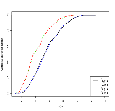
The majority of cluster sizes are $d=10$ and although some are $d=9$ in the actual data. The bootstrap monitoring test can be carried out without any difficulties. Table 8 includes all the information needed for the proposed monitoring test. Clearly, the data analysis leads to solid evidence against both $H_{0}:\xi_{0,0.05}-\xi_{1,0.05}=0$ and $H_{0}:\xi_{0,0.1}-\xi_{1,0.1}=0$ in favour of one-sided alternatives: $H_{a}:\xi_{0,0.05}-\xi_{1,0.05}>0$ or $H_{a}:\xi_{0,0.1}-\xi_{1,0.1}>0$. We confidently conclude that the 2011/2012 population has lower quality index values than the in-Grade population. Based on the theory developed in this paper, the risk of false alarm based on this analysis is low.

Table 8: Composite EL estimates and bootstrap confidence intervals of $\Delta\xi_{0,1,\alpha}=\xi_{0,\alpha}-\xi_{1,\alpha}$

$\mbox{\bf q}(y)$	Point Estimate		95% one-sided CI		99% one-sided CI
	$\Delta\xi_{0,1,0.05}$	$\Delta\xi_{0,1,0.10}$	$\Delta\xi_{0,1,0.05}$	$\Delta\xi_{0,1,0.10}$	$\Delta\xi_{0,1,0.05}$	$\Delta\xi_{0,1,0.10}$
$(1,\log y)^{\tau}$	0.677	0.903	$[0.508,\infty)$	$[0.650,\infty)$	$[0.438,\infty)$	$[0.563,\infty)$
$(1,y,\log y)^{\tau}$	0.695	0.916	$[0.497,\infty)$	$[0.642,\infty)$	$[0.416,\infty)$	$[0.535,\infty)$
$(1,\log y,\log^{2}y)^{\tau}$	0.734	0.922	$[0.515,\infty)$	$[0.659,\infty)$	$[0.429,\infty)$	$[0.552,\infty)$

6 Summary and discussion

We have presented a bootstrap composite EL monitoring test for multiple samples with a clustered structure. The composite EL is effective, the cluster-based bootstrap confidence intervals have satisfactory precise coverage probabilities, and the monitoring test controls type I error rates tightly with good power. We have shown these points through simulation studies and a real example. Further improvements in the precision of the coverage probability and type I error rates are possible. We aim to refine the current results along the lines of Loh (1991) and Ho and Lee (2005) in the future.

7 Acknowledgement

We are indebted to Drs. Steve Verrill, David Kretschmann, James Evans at the United States Forest Products Lab for making their report available as well as for providing the dataset on which their analyses and now ours are based. We are also indebted to members of the Forest Products Stochastic Modelling Group centered at the University of British Columbia (UBC), from FPInnovations in Vancouver, Simon Fraser University and UBC for stimulating discussions on the long term monitoring program to which this paper is addressed.

Appendix: Proofs

Proof of Theorem 1

Theorem 1 is useful because it links the limiting distribution of the composite EL quantiles $\hat{\xi}_{r}$ to that of the composite cdf  $\hat{G}_{r}(\xi_{r})$ for one of the $m+1$ populations, $G_{r}(y)$, and the specific level $\xi_{r}$ of the quantile. We give a proof based on the following lemma, which will be proved subsequently.

Lemma 1.

Under the conditions of Theorem 1, $\hat{}\mbox{\boldmath$\theta$}-\mbox{\boldmath$\theta$}_{0}=O_{p}(n^{-1/2})$ and $\hat{\xi}_{r}-\xi_{r}=O_{p}(n^{-1/2})$.

Let $a_{n}=cn^{-1/2}\log^{1/2}n$ for some $c>0$. Under Lemma 1, the conclusion of Theorem 1 is implied by

$$\sup_{y:~{}|y-\xi_{r}|<a_{n}}|\{\hat{G}_{r}(y)-\hat{G}_{r}(\xi_{r})\}-\{G_{r}(y)-G_{r}(\xi_{r})\}|=O_{p}(n^{-3/4}\log^{3/4}n).$$ (A.1)

We comment that the choice of $a_{n}$ is for convenience of presentation. It guarantees that with probability approaching 1, the $a_{n}$-neighbourhood of $\xi_{r}$ contains $\hat{\xi}_{r}$. The power $1/2$ of $\log n$ in $a_{n}$ is not essential; any positive value no larger than $1/2$ will do.

Proof of Theorem 1 . We first work on (A.1) after $G_{k}$ is replaced by $\tilde{G}_{k}$ where

$$\tilde{G}_{k}(y)=d^{-1}\sum_{l=1}^{d}\big{\{}n_{k}^{-1}\sum_{j=1}^{n_{k}}h_{k}(y_{k,j,l};\mbox{\boldmath$\theta$}_{0})\mathbbm{1}(y_{k,j,l}\leq y)\big{\}}=d^{-1}\sum_{l=1}^{d}\tilde{G}_{k,l}(y)$$

with $\tilde{G}_{k,l}(y)=n_{k}^{-1}\sum_{j=1}^{n_{k}}h_{k}(y_{k,j,l};\mbox{\boldmath$\theta$}_{0})\mathbbm{1}(y_{k,j,l}\leq y)$. Because the clusters are independent of each other and each is made of $d$ exchangeable units, $\tilde{G}_{k,l}(y)$ for each $k$ and $l$ is a standard empirical distribution function.

Without loss of generality we consider only the case where $y\geq\xi_{0}$. We have

$$\big{|}\{\hat{G}_{r}(y)-\hat{G}_{r}(\xi_{r})\}-\{\tilde{G}_{r}(y)-\tilde{G}_{r}(\xi_{r})\}\big{|}$$ (A.2)

$$\leq (n_{r}d)^{-1}\sum_{k,j,l}\{|h_{r}(y_{k,j,l};\hat{}\mbox{\boldmath$\theta$})-h_{r}(y_{k,j,l};\mbox{\boldmath$\theta$}_{0})|\}\mathbbm{1}(\xi_{r}<y_{k,j,l}\leq y)$$

$$\leq (n_{r}d)^{-1}\{\|\hat{}\mbox{\boldmath$\theta$}-\mbox{\boldmath$\theta$}_{0}\|\}\sum_{k,j,l}\{\|\mbox{\bf q}(y_{k,j,l})\|\mathbbm{1}(\xi_{r}<y_{k,j,l}\leq y)\}$$

by the mean value theorem and the Cauchy–Schwarz inequality, where $\|\cdot\|$ denotes the $L_{2}$-norm. Let

$$X_{k,j,l}=\|\mbox{\bf q}(y_{k,j,l})\|\mathbbm{1}(\xi_{r}<y_{k,j,l}\leq\xi_{r}+a_{n}).$$

Because the indicator function has both mean and variance of order $a_{n}$, and $\mbox{\bf q}(\cdot)$ has finite moments as implied by C3, we have

$${\mathbb{E}}(X_{k,j,l})=O(a_{n})\mbox{ and }{\mathbb{V}\rm ar}(X_{k,j,l})\leq{\mathbb{E}}(X_{k,j,l}^{2})=O(a_{n}).$$

Because observations from different clusters are independent, the above calculations lead to $\sum_{k,j,l}X_{k,j,l}=O(na_{n}).$ Furthermore, we get

$$\sup_{\xi_{r}\leq y\leq\xi_{r}+a_{n}}\sum_{k,j,l}\{\|\mbox{\bf q}(y_{k,j,l})\|\mathbbm{1}(\xi_{r}<y_{k,j,l}\leq y)\}\leq\sum_{k,j,l}X_{k,j,l}=O_{p}(na_{n}).$$

Combining this with $\hat{}\mbox{\boldmath$\theta$}-\mbox{\boldmath$\theta$}_{0}=O(n^{-1/2})$ and (A.2), we get

$$\sup_{\xi_{r}\leq y\leq\xi_{r}+a_{n}}|\{\hat{G}_{r}(y)-\hat{G}_{r}(\xi_{r})\}-\{\tilde{G}_{r}(y)-\tilde{G}_{r}(\xi_{r})\}|=O_{p}(n^{-1}\log^{1/2}n),$$

which is sufficiently small compared with $n^{-3/4}\log^{3/4}n$ in (A.1).

Our final task is to replace $\tilde{G}_{r}$ in the above conclusion by $G_{r}$ after the order is relaxed to $n^{-3/4}\log^{3/4}n$. Since $\tilde{G}_{r,l}(y)$ is an empirical distribution based on iid  random variables, for each $l$, we have

$$\sup_{\xi_{r}\leq y\leq\xi_{r}+a_{n}}|\{\tilde{G}_{r,l}(y)-\tilde{G}_{r,l}(\xi_{r})\}-\{G_{r}(y)-G_{r}(\xi_{r})\}|=O_{p}(n^{-3/4}\log^{3/4}n).$$ (A.3)

The result can be proved following Lemma 2.5.4E in Serfling (1980; p. 97); we omit the details. Intuitively, the difference is of order $O_{p}(n^{-1/2})$ uniformly in $y$. When $y$ is restricted to an $a_{n}$-neighbourhood, its size is reduced by a factor of $\sqrt{a_{n}\log n}$ as given above. Therefore,

$$\sup_{\xi_{r}\leq y\leq\xi_{r}+a_{n}}|\{\tilde{G}_{r}(y)-\tilde{G}_{r}(\xi_{r})\}-\{G_{r}(y)-G_{r}(\xi_{r})\}|$$

$$\leq \sup_{\xi_{r}\leq y\leq\xi_{r}+a_{n}}\max_{1\leq l\leq d}|\{\tilde{G}_{r,l}(y)-\tilde{G}_{r,l}(\xi_{r})\}-\{G_{r}(y)-G_{r}(\xi_{r})\}|$$

$$= O_{p}(n^{-3/4}\log^{3/4}n).$$

Since $\hat{\xi}_{r}=\xi_{r}+O_{p}(n^{-1/2})$, which is within the $a_{n}$-neighbourhood of $\xi_{r}$, the above bound is applicable to $y=\hat{\xi}_{r}$, which leads to the conclusion. This completes the proof of Theorem 1. ∎

Proof of Lemma 1 For $l=1,2,\ldots,d$, define

$$\ell_{l}(\mbox{\boldmath$\theta$})=-\sum_{k,j}\log\big{[}\sum_{r=0}^{m}\rho_{r}\exp\{\mbox{\boldmath$\theta$}_{r}^{\tau}\mbox{\bf q}(y_{k,j,l})\}\big{]}+\sum_{k,j}\mbox{\boldmath$\theta$}_{k}^{\tau}\mbox{\bf q}(y_{k,j,l}).$$

Note that the range of the summation holds $l$ fixed. It can be seen that

$$\ell_{n}(\mbox{\boldmath$\theta$})=\sum_{l=1}^{d}\ell_{l}(\mbox{\boldmath$\theta$}).$$

Given $l$, $\ell_{l}(\mbox{\boldmath$\theta$})$ is a profile EL function of $\theta$ based on one observation from each cluster in the data set. These observations form a new data set with cluster size $d=1$. Hence, each $\ell_{l}(\mbox{\boldmath$\theta$})$ is a profile EL function under DRM, the same as that given in Chen and Liu (2013). To save space, we cite their Lemma A.1, which states that for any $\theta$ such that $\mbox{\boldmath$\theta$}=\mbox{\boldmath$\theta$}_{0}+o(n^{-1/3})$ we have

$$\ell_{l}(\mbox{\boldmath$\theta$})-\ell_{l}(\mbox{\boldmath$\theta$}_{0})=(\mbox{\boldmath$\theta$}-\mbox{\boldmath$\theta$}_{0})^{\tau}\mbox{\bf Z}_{n.l}-\frac{n}{2}(\mbox{\boldmath$\theta$}-\mbox{\boldmath$\theta$}_{0})^{\tau}\mbox{\bf W}(\mbox{\boldmath$\theta$}-\mbox{\boldmath$\theta$}_{0})+o_{p}(1)$$

for each $l$, where $n^{-1/2}\mbox{\bf Z}_{n,l}$ is asymptotic normal and W was defined just before Theorem 2. Note that $\mbox{\boldmath$\theta$}_{0}$ instead of $\mbox{\boldmath$\theta$}^{*}$ is the true parameter value here, to avoid possible confusion with the bootstrap notation.

These decompositions imply that $\ell_{n}(\mbox{\boldmath$\theta$})=\sum_{l=1}^{d}\ell_{l}(\mbox{\boldmath$\theta$})$ has a local maximum within an $o(n^{-1/3})$-neighbourhood of $\mbox{\boldmath$\theta$}_{0}$ in probability. Because $\ell_{n}(\mbox{\boldmath$\theta$})$ is concave, this local maximum is in fact global. Furthermore, it must satisfy

$$n^{1/2}(\hat{}\mbox{\boldmath$\theta$}-\mbox{\boldmath$\theta$}_{0})=n^{-1/2}\mbox{\bf W}^{-1}\big{\{}d^{-1}\sum_{l=1}^{d}\mbox{\bf Z}_{n,l}\big{\}}+o_{p}(1)=O_{p}(1).$$

This proves that $\hat{}\mbox{\boldmath$\theta$}-\mbox{\boldmath$\theta$}_{0}=O_{p}(n^{-1/2})$, the first conclusion of the lemma.

The second conclusion of the lemma is implied by

$$\sup_{y}|\hat{G}_{r}(y)-G_{r}(y)|=O_{p}(n^{-1/2}),$$

or, for $l=1,2,\ldots,d$,

$$\sup_{y}|\hat{G}_{r,l}(y)-G_{r}(y)|=O_{p}(n^{-1/2})$$ (A.4)

because $\hat{G}_{r}(y)=d^{-1}\sum_{l=1}^{d}\hat{G}_{r,l}(y)$. Since

$$\sup_{y}|\hat{G}_{r,l}(y)-G_{r}(y)|\leq\sup_{y}|\hat{G}_{r,l}(y)-\tilde{G}_{r,l}(y)|+\sup_{y}|\tilde{G}_{r,l}(y)-G_{r}(y)|,$$

to prove (A.4) it suffices to show that

$$\sup_{y}|\hat{G}_{r,l}(y)-\tilde{G}_{r,l}(y)| = O_{p}(n^{-1/2})\quad\mbox{and}$$ (A.5)

$$\sup_{y}|\tilde{G}_{r,l}(y)-G_{r}(y)| = O_{p}(n^{-1/2}).$$ (A.6)

Note that the sum in $\tilde{G}_{r,l}(y)=n_{r}^{-1}\sum_{k,j}h_{r}(y_{j,k,l};\mbox{\boldmath$\theta$}_{0})\mathbbm{1}(y_{j,k,l}\leq y)$ contains exactly one observation from every cluster. Hence, it also reduces to the case where the cluster size $d=1$, and (A.6) was proved by Chen and Liu (2013).

Remark: Chen and Liu (2013) overlooked a technical detail. They thought that (A.6) is directly implied by the simpler nonuniform result $\tilde{G}_{r,l}(y)-G_{r}(y)=O_{p}(n^{-1/2})$. This is not true, but (A.6) can be proved with one extra step as follows. For any Donsker class ${\mathcal{H}}$ of functions, it is known that

$$\sup_{h\in\mathcal{H}}|n^{-1}\sum_{i=1}^{n}h(y_{i})-{\mathbb{E}}\{h(Y)\}|=O_{p}(n^{-1/2})$$

when $y_{1},y_{2},\ldots,y_{n}$ is an iid  sample from the population of $Y$. Because $0\leq h_{r}(y;\mbox{\boldmath$\theta$}_{0})\leq 1$, ${\mathcal{H}}=\{h_{r}(y;\mbox{\boldmath$\theta$}_{0})\mathbbm{1}(y\leq t):t\in\mbox{$\mathcal{R}$}\}$ is a Donsker function class (function of $y$). The verification directly follows Example 2.10.10 of van der Vaart and Wellner (1996, p. 192). Applying this property to ${\mathcal{H}}$ leads to (A.6).

The remaining task is to prove (A.5). We may cite Chen and Liu (2013) or directly verify

$$\sup_{y}|\hat{G}_{r,l}(y)-\tilde{G}_{r,l}(y)|\leq n_{r}^{-1}\sum_{k,j,l}\|\mbox{\bf q}(y_{k,j,l})\|\times\|\hat{}\mbox{\boldmath$\theta$}-\mbox{\boldmath$\theta$}_{0}\|=O_{p}(\|\hat{}\mbox{\boldmath$\theta$}-\mbox{\boldmath$\theta$}_{0}\|)=O_{p}(n^{-1/2}).$$

This completes the proof of Lemma 1. ∎

Proof of Theorem 2

For $l=1,\ldots,d$, the proof of Theorem 3.2 of Chen and Liu (2013) claims that

$$\hat{G}_{r,l}(y)-G_{r}(y) = n_{r}^{-1}\sum_{k,j}[h_{r}(y_{k,j,l})I(y_{k,j,l}\leq y)-{\mathbb{E}}\{h_{r}(y_{k,j,l})I(y_{k,j,l}\leq y)\}]$$

$$+n_{r}^{-1}\mbox{\bf B}_{r}^{\tau}(y)\mbox{\bf W}^{-1}\mbox{\bf Z}_{n,l}+o_{p}(n^{1/2}).$$

Explicitly, $\mbox{\bf Z}_{n,l}$ is a long vector with its $r$th segment being

$$\mbox{\bf Z}_{n,r,l}=\sum_{k,j}[\{\delta_{kr}-h_{r}(y_{k,j,l})\}\mbox{\bf q}(y_{k,j,l})].$$ (A.7)

The message is that it is a sum of independent random variables with overall mean $0$. This structure implies that $\hat{G}_{r}(y)=d^{-1}\sum_{l}\hat{G}_{r,l}(y)$ has the claimed asymptotic normality. The specific covariance structure in the theorem arises because $\hat{G}_{r,l,1}(y)$ and $\hat{G}_{r,l,2}(y)$ are correlated as a result of the cluster structure.

Proof of Theorem 3

The conclusion of this theorem is easily implied by Theorems 1 and 2.

Proof of Theorem 4

Recall that for each fixed $l$, we defined

$$\tilde{G}_{r,l}^{*}(y)=n_{k}^{-1}\sum_{j=1}^{n_{k}}h_{k}(y^{*}_{k,j,l};\mbox{\boldmath$\theta$}_{0})\mathbbm{1}(y^{*}_{k,j,l}\leq y),$$

which is the bootstrap version of $\tilde{G}_{r,l}(y)$. In the same spirit, let

$$\hat{G}_{r}(y)=d^{-1}\sum_{l=1}^{d}\hat{G}_{r,l}(y);~{}~{}\hat{G}_{r}^{*}(y)=d^{-1}\sum_{l=1}^{d}\hat{G}_{r,l}^{*}(y).$$

The conclusions of the following lemma are parallel to those of Lemma 1. The proof is almost the same and therefore omitted.

Lemma 2.

Under the conditions of Theorem 1, we have

$$\hat{\mbox{\boldmath$\theta$}}^{*}-{{\mbox{\boldmath$\theta$}}_{0}}=O_{p}(n^{-1/2});~{}~{}~{}\hat{\xi}_{r}^{*}-{{\xi}_{r}}=O_{p}(n^{-1/2}).$$

The next lemma contains key intermediate results for the proof of Theorem 4.

Lemma 3.

Assume the conditions of Theorem 1. Let $a_{n}=cn^{-1/2}\log^{1/2}n$ for an arbitrary $c>0$. Then, uniformly over $y:|y-\xi_{r}|\leq a_{n}$ the following quantities

$$\{\hat{G}_{r}^{*}(y)-\hat{G}_{r}^{*}(\xi_{r})\},\{\tilde{G}_{r}^{*}(y)-\tilde{G}_{r}^{*}(\xi_{r})\},\{\tilde{G}_{r}(y)-\tilde{G}_{r}(\xi_{r})\},{\{G_{r}(y)-G_{r}(\xi_{r})\}}$$

are within $O_{p}(n^{-3/4}\log^{3/4}n)$ distance of each other.

Remark: The choice of $a_{n}$ ensures that the $a_{n}$-neighbourhood of $\xi_{r}$ covers $\hat{\xi}^{*}_{r}$ and so on, based on the results of Lemma 2.

Proof of Lemma 3. Since the cluster-based bootstrap preserves the cluster structure, it suffices to establish the claimed closeness for each $l$. That is, we need work only on the case where the cluster size $d=1$. Thus, we have dropped the subscript $l$ from $\hat{G}_{r,l}^{*}(y)$ and $y_{k,j,l}$. Note that

$$\sup_{y:~{}|y-\xi_{r}|<a_{n}}|\{\hat{G}_{r}^{*}(y)-\hat{G}_{r}^{*}(\xi_{r})\}-\{\tilde{G}_{r}^{*}(y)-\tilde{G}_{r}^{*}(\xi_{r})\}|$$

$$\leq n_{r}^{-1}\|\hat{}\mbox{\boldmath$\theta$}^{*}-\mbox{\boldmath$\theta$}_{0}\|\sum_{k,j}\|\mbox{\bf q}(y^{*}_{k,j})\|\mathbbm{1}(|\xi_{r}-y^{*}_{k,j}|\leq a_{n})$$

$$\leq \|\hat{}\mbox{\boldmath$\theta$}^{*}-\mbox{\boldmath$\theta$}_{0}\|\{n_{r}^{-1}\sum_{k,j}\|\mbox{\bf q}(y^{*}_{k,j})\|^{2}\}^{1/2}\{n_{r}^{-1}\sum_{k,j}\mathbbm{1}(|\xi_{r}-y^{*}_{k,j}|\leq a_{n})\}^{1/2}$$

$$= O(n^{-3/4}\log^{1/4}n)$$

because $\|\hat{}\mbox{\boldmath$\theta$}^{*}-\mbox{\boldmath$\theta$}_{0}\|=O_{p}(n^{-1/2})$ for the first factor, the second factor is $O_{p}(1)$, and the last term is $O_{p}(n^{-1/4}\log^{1/4}n)$. This proves the closeness of the first two random entities in the lemma.

We now prove the closeness of the second and third entities. Note that for $y>\xi_{r}$ (and similarly for $y<\xi_{r}$),

$$\tilde{G}_{r}^{*}(y)-\tilde{G}_{r}^{*}(\xi_{r})=\sum_{k,j}h_{r}(y^{*}_{k,j};\mbox{\boldmath$\theta$}_{0})\mathbbm{1}(\xi_{r}<y^{*}_{k,j}\leq y),$$

in which the summands are composed of $m+1$ conditionally iid  bootstrap samples. Each summand is bounded between 0 and 1. We may therefore apply the technique of the Bernstein inequality (Serfling, 1980; p. 85) and the techniques in the proof of Lemma 2.5.4E of Serfling (1980; p. 97) to show that

$$\sup_{y:~{}|y-\xi_{r}|<a_{n}}|\{\tilde{G}_{r}^{*}(y)-\tilde{G}_{r}^{*}(\xi_{r})\}-{\mathbb{E}}^{*}\{\tilde{G}_{r}^{*}(y)-\tilde{G}_{r}^{*}(\xi_{r})\}|=O_{p}(n^{-3/4}\log^{3/4}n)$$

where ${\mathbb{E}}^{*}$ is the bootstrap expectation.

Our order assessment is not tight, and we require only an “in probability” rather than an “almost surely” ordering. Interested readers can easily verify this conclusion based on the cited work, but the details are tedious and are omitted here.

The conditional iid  structure leads to

$${\mathbb{E}}^{*}\{\tilde{G}_{r}^{*}(y)\}=\tilde{G}_{r}(y)=n_{k}^{-1}\sum_{j=1}^{n_{k}}h_{r}(y_{k,j};\mbox{\boldmath$\theta$}_{0})\mathbbm{1}(y_{k,j}\leq y).$$

This proves the closeness of the second and third entities.

The closeness of the third and fourth entities is given by (A.3). ∎

Proof of Theorem 4.

Employing the results in Lemma 3, we have

$$\sup_{y:~{}|y-\xi_{r}|<a_{n}}|\{\hat{G}_{r}^{*}(y)-\hat{G}_{r}^{*}(\xi_{r})\}-\{G_{r}(y)-G_{r}(\xi_{r})\}|=O_{p}(n^{-3/4}\log^{3/4}n).$$ (A.8)

Combining Lemma 2 and (A.8), we conclude that $\hat{\xi}_{r}^{*}$ admits a Bahadur representation as follows:

$$\hat{\xi}_{r}^{*}=\xi_{r}+\{{\alpha}-\hat{G}_{r}^{*}(\xi_{r})\}/g_{r}(\xi_{r})+O_{p}(n^{-3/4}\log^{3/4}n).$$ (A.9)

From Theorem 1, we can easily deduce that

$$\sqrt{n}(\hat{\xi}^{*}_{r}-\hat{\xi}_{r})=\frac{\sqrt{n}\{\hat{G}_{r}^{*}(\xi_{r})-\hat{G}_{r}(\xi_{r})\}}{g_{r}(\xi_{r})}+o_{p}(1).$$

Note that asymptotically both $\hat{G}_{r}^{*}(\xi_{r})$ and $\hat{G}_{r}(\xi_{r})$ are simple linear combinations of some sample means. Hence, it is a standard bootstrap conclusion (Singh, 1981; Hall, 1986; Shao and Tu, 1995) that the distribution of $\sqrt{n}\{\tilde{G}_{r}^{*}(\xi_{r})-\tilde{G}_{r}(\xi_{r})\}$ is well approximated by that of $\sqrt{n}\{\tilde{G}_{r}(\xi_{r})-G_{r}(\xi_{r})\}$.

By the Slutsky theorem (Serfling, 1980, p. 85) and the conditional Slutsky theorem (Cheng, 2015), the bootstrap conclusion extends to differentiable functions of $\xi_{r}$, $\xi_{s}$, and beyond. Hence, we get the conclusion of this theorem. ∎