Mechanical Graphene

Abstract

We present a model of a mechanical system with a vibrational mode spectrum identical to the spectrum of electronic excitations in a tight-binding model of graphene. The model consists of point masses connected by elastic couplings, called “tri-bonds,” that implement certain three-body interactions, which can be tuned by varying parameters that correspond to the relative hopping amplitudes on the different bond directions in graphene. In the mechanical model, this is accomplished by varying the location of a pivot point that determines the allowed rigid rotations of a single tri-bond. The infinite system constitutes a Maxwell lattice, with the number of degrees of freedom equal to the number of constraints imposed by the tri-bonds. We construct the equilibrium and compatibility matrices and analyze the model’s phase diagram, which includes spectra with Weyl points for some placements of the pivot and topologically polarized phases for others. We then discuss the edge modes and associated states of self stress for strips cut from the periodic lattice. Finally, we suggest a physical realization of the tri-bond, which allows access to parameter regimes not available to experiments on (strained) graphene and may be used to create other two-dimensional mechanical metamaterials with different spectral features.

I Introduction

Topology Nakahara2003 ; volovik03 ; Volovik2007 has become an important tool in advancing our understanding of electronic properties of solids. It plays an important role, for example, in determining the nature of surface states in a wide variety of systems including polyacetylene ssh ; jackiw76 , quantum Hall systems halperin82 ; haldane88 , and topological insulators km05b ; bhz06 ; mb07 ; fkm07 ; HasanKane2010 ; QiZhang2011 . The success in applying topological ideas to electronic systems has recently inspired their generalization to certain classes of classical mechanical systems KaneLub2014 ; LubenskySun2015 ; PauloseVit2015 ; PauloseVit2015-b ; ChenVit2014 ; VitelliChe2014 ; Chen2015 ; Xiao2015 ; Po2014 ; Yang2015 ; Nash2015 ; Wang2015 ; Wang2015a ; Susstrunk2015 ; Kariyado2015 ; Peano2015 ; Mousavi2015 ; Khanikaev2015 ; RocklinLub2016 by establishing a correspondence between quantum electronic Hamiltonians and the “square root” of the mechanical dynamical matrix. This correspondence is exact for a class of Maxwell lattices for which there is a balance between the number of degrees of freedom and the number of constraints per unit cell. A prototype example is the one-dimensional mechanical model KaneLub2014 ; ChenVit2014 ; ZhouVitelli2016 whose excitation spectrum precisely matches the spectrum of the Su-Schrieffer-Heeger (SSH) model for polyacetylene. In the one-dimensional SSH model, electrons move on a bipartite lattice with different hopping matrix elements on alternating bonds that connect the sites on the $A$- and $B$-sublattice. The mechanical model consists of rigid rotors with pivot points fixed on the $A$-sublattice and connected by central-force springs residing on the the $B$-sublattice. There is a one-to-one correspondence between electrons on the $A$-sublattice in the SSH model and the rotors in mechanical model and between electrons on the $B$-sublattice and the springs of the mechanical model. We note that in contrast to other models of topological mechanics Yang2015 ; Nash2015 ; Wang2015 ; Wang2015a ; Susstrunk2015 ; Kariyado2015 ; Peano2015 ; Mousavi2015 ; Khanikaev2015 Maxwell lattices exhibit topologically protected zero frequency modes, along with an intrinsic particle-hole symmetry in the analog quantum Hamiltonian.

Here, we introduce and explore the properties of a model mechanical system whose bulk vibrational excitations are in correspondence with the electronic excitations of the particle-hole symmetric two-band tight-binding model of graphene. We consider a generalized graphene model describing nearest neighbor hopping on a honeycomb lattice in which the hopping matrix elements for the three bonds emanating from a given site are in general different. This model can represent strained graphene KaneMele1997 for modest variations in the hopping amplitudes, and also arises in the analysis of Kitaev’s honeycomb lattice model Kitaev2006 . Our mechanical analog is constructed by closely following the paradigm used in the construction of the SSH analog. The honeycomb lattice of graphene, like the 1D SSH lattice, is bipartite with $A$- and $B$-sublattices, shown as red and blue disks in Fig. 1. Since there is only one degree of freedom per site in the graphene model, we assign a scalar variable $z({\bm{R}}_{A})$, which we identify as vertical height displacement, to each site on the $A$-sublattice, and we assign a kinetic energy $\dot{z}^{2}({\bm{R}}_{A})/2$ to that site. On each site in the $B$-sublattice, we need to assign the analog of a bond connecting sites on the $A$-sublattice, but this “bond” is connected to three rather than the usual two sites. To each of these triangular bonds, which we call tri-bonds, we assign a kind of “stretching” energy that depends quadratically on a certain linear combination of the heights at the three sites.

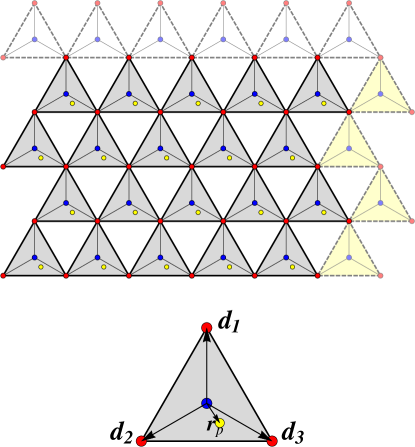
Figure 1: Top: The tri-bond lattice. Each shaded triangle represents a tri-bond centered on a $B$ site of the graphene lattice (blue disks). The tri-bonds are connected at their vertices, which lie on $A$-sublattice (red disks). The yellow disk in each tri-bond marks the pivot point. Dashed tri-bonds are those that are cut to create free surfaces. Bottom: A single tri-bond. The pivot point ${\bm{r}}_{p}$ is at $(x_{1}{\bm{d}}_{1}+x_{2}{\bm{d}}_{2}+x_{3}{\bm{d}}_{3})$.

Figure 1 shows our model mechanical graphene lattice, with red sites representing the locations of the height variables and gray triangles representing the tri-bonds.

The tri-bonds are the analogs of springs in a standard ball-and-spring lattice, and each imposes a constraint that leads to a generalization of the Maxwell-Calladine theorem Calladine1978 relating the numbers of zero modes and states of self stress (SSS) to the number of degrees of freedom and number of constraints. Under periodic boundary conditions, our mechanical graphene lattice is a generalized Maxwell lattice LubenskySun2015 ; Calladine1978 in which the number of constraints equals the number of degrees of freedom, and it exhibits all of the properties of ball-and-spring Maxwell lattices: (1) Each zero mode in the bulk spectrum, which again matches the electronic spectrum of graphene, is accompanied by a SSS. (2) Each lattice is characterized by a topological polarization or by Weyl modes. (3) Periodic strips or finite lattices cut from a periodic lattice whose spectrum is fully gapped have a number of zero-frequency surface modes equal to the number of tri-bonds cut, i.e., at least one zero mode per surface wavenumber, residing on one or the other of the opposite free edges. (4) The number of zero modes at a given wavenumber on a free surface is determined by the topological polarization or by the positions of Weyl modes and by a local surface polarization. (5) Domain walls connecting lattices of different topological polarization harbor either zero modes or self stress for each wavenumber along the wall; those connecting different Weyl lattices have zero modes or states of self stress for some wavenumbers but not for others.

Though the bulk spectrum of our model and graphene are identical, their surfaces modes are not. The top and bottom edges of a horizontal strip of the mechanical lattice, which can be created by removing the row of horizontal of dashed tri-bonds in Figure 1 from a periodic lattice, are different: the top surface exposes tri-bond vertices and the bottom a straight continuous line of tri-bond edges. These two surfaces correspond, respectively, to the bearded (with dangling bonds) and zigzag edges of graphene Kohmoto2007 . It is not possible to create a strip in the mechanical lattice like that in graphene in which both edges are zigzagged. Both edges of vertical strips exhibit a two-tri-bond zigzag pattern. The corresponding graphene edges correspond to armchair edges with an extra dangling bond at every second row.

This paper is divided into five sections of which this is the first. Section II presents details of our model and defines the equilibrium and compatibility matrices that establish the Maxwell-Calladine theorem. Section III treats the excitation spectrum and establishes a phase diagram with a region harboring Weyl points and regions that carry a topological polarization. Section IV discusses zero modes at free edges or in domain walls. Section V presents physical models for the tri-bonds.

II Mechanical Graphene Model

Figure 1 provides a visual image of our model. We take the Bravais lattice constant to be $a$ and define primitive reciprocal lattice vectors

$${\bf a}_{1} = a\hat{x},$$ (1)

$${\bf a}_{2} = a(-{1\over 2}\hat{x}+{\sqrt{3}\over 2}\hat{y}),$$ (2)

$${\bf a}_{3} = a(-{1\over 2}\hat{x}-{\sqrt{3}\over 2}\hat{y}).$$ (3)

We also define the three vectors from a tri-bond centroid to its vertices:

$${\bf d}_{1} = {a\over\sqrt{3}}\hat{y}$$ (4)

$${\bf d}_{2} = {a\over\sqrt{3}}(-{\sqrt{3}\over 2}\hat{x}-{1\over 2}\hat{y})$$ (5)

$${\bf d}_{3} = {a\over\sqrt{3}}({\sqrt{3}\over 2}\hat{x}-{1\over 2}\hat{y}).$$ (6)

The centroids of the tri-bonds are located on $B$ sites of the honeycomb and their vertices lie at $A$ sites. Each site on the $A$-sublattice is occupied by a unit mass that is constrained (say by a frictionless rod) to move in the vertical direction. We assume these vertical displacements $z({\bm{R}}_{A})$ are small enough that linear approximations can be used. Each tri-bond is pinned at a pivot point that is displaced from its centroid by

$${\bm{r}}_{p}=x_{1}{\bm{d}}_{1}+x_{2}{\bm{d}}_{2}+x_{3}{\bm{d}}_{3},$$ (7)

and the three tri-bonds meeting at a given site are connected in a way that allows each to freely rotate about an axis passing through its pivot point and the site in question.

Any location of the pivot point (within or outside the triangle spanned by the tri-bond vertices) can be specified by a unique triple $x=(x_{1},x_{2},x_{3})$ with $x_{1}+x_{2}+x_{3}=1$. With this parametrization, the condition

$$e({\bm{R}}_{B})\equiv\sum_{i=1}^{3}x_{i}z({\bm{R}}_{B}+{\bm{d}}_{i})=0,$$ (8)

is satisfied for any rigid rotation of the tri-bond, where ${\bm{R}}_{B}$ is the $B$-sublattice location of the tri-bond centroid and ${\bm{R}}_{B}+{\bm{d}}_{i}$ are the $A$-sublattice positions of the vertices of the tri-bond. Violations of this condition necessarily cause a distortion of the tri-bond that costs some energy, which to lowest order in displacements must be quadratic in $e({\bm{R}}_{B})$, giving us an elastic energy

$$U=\frac{1}{2}k\sum_{B}e^{2}({\bm{R}}_{B})$$ (9)

where the sum is over all sites ${\bm{R}}_{B}$ in the $B$-sublattice. This energy has exactly the same form as that of a lattice of harmonic springs where the sum is over bonds and $e$ is the elongation of a bond. Following this analogy, we call $e({\bm{R}}_{B})$ the stretch of the tri-bond at ${\bm{R}}_{B}$. Of course, with the aid of Eq. (8) we can express $U$ as a function of the displacements $z({\bm{R}}_{A})$ instead of stretches $e({\bm{R}}_{B})$.

Given $U$, we can now construct expressions for the $N_{B}$ tri-bond tensions $t({\bm{R}}_{B})$ conjugate to stretches of the tri-bonds and the $N$ site forces $f({\bm{R}}_{A})$ conjugate to vertical displacements of the masses:

$$t({\bm{R}}_{B}) = \frac{\partial U}{\partial e({\bm{R}}_{B})}=ke({\bm{R}}_{B})$$ (10)

$$= k\sum_{i}x_{i}z({\bm{R}}_{A}+{\bm{d}}_{i})$$

$$f({\bm{R}}_{A}) = \frac{\partial U}{\partial z({\bm{R}}_{A})}=k\sum_{i}x_{i}e({\bm{R}}_{A}-{\bm{d}}_{i})$$ (11)

$$= \sum_{i}x_{i}t({\bm{R}}_{A}-{\bm{d}}_{i}).$$

The tension $t$ is one that induces “stretching” of the tri-bond in a manner exactly analogous to the tension in a spring bond inducing stretching of the spring. The tri-bond stretch is a measure of the deviation from coplanarity of its three vertices and pivot point.

Introducing the $N$-dimensional vectors ${\bm{z}}$ and ${\bm{f}}$ of site-displacements and forces and the $N_{B}$ dimensional vectors of ${\bm{e}}$ and ${\bm{t}}$ of stretches and tensions, we can write Eqs. (8), (10), and (11) as

$${\bm{e}}=C{\bm{z}};\qquad{\bm{t}}=k{\bm{e}};\qquad{\bm{f}}=Q{\bm{t}},$$ (12)

where $C$ is the compatibility matrix with components

$$C({\bm{R}}_{B},{\bm{R}}_{A})=\sum_{i}x_{i}\delta_{{\bm{R}}_{B}+{\bm{d}}_{i},{\bm{R}}_{A}},$$ (13)

and $Q$ is the equilibrium matrix with components

$$Q({\bm{R}}_{A},{\bm{R}}_{B})=\sum_{i}x_{i}\delta_{{\bm{R}}_{A}-{\bm{d}}_{i},{\bm{R}}_{B}}.$$ (14)

$Q=C^{T}$ as required. In Fourier space,

$$e({\bm{q}})=C({\bm{q}})z({\bm{q}});\qquad f({\bm{q}})=Q({\bm{q}})t({\bm{q}}),$$ (15)

where $C({\bm{q}})$ and $Q({\bm{q}})$ in this case are $1\times 1$ matrices with

$$C({\bm{q}})=\sum_{i}x_{i}e^{i{\bm{q}}\cdot{\bm{d}}_{i}}=Q^{*}({\bm{q}}).$$ (16)

As in the case of central-force springs, the null space of $C$ consists of zero modes and that of $Q$ of SSSs. The global and wave-number specific Maxwell-Calladine index theorems LubenskySun2015 follow immediately:

$$N_{0}-S=N-N_{B}$$ (17)

and

$$n_{0}({\bm{q}})-s({\bm{q}})=n-n_{B},$$ (18)

where $N_{0}$ and $S$ are, respectively, the total number of zero modes and the total number of SSSs, $n_{0}({\bm{q}})$ and $s({\bm{q}})$ are the numbers of zero modes and states of self stress at wavenumber ${\bm{q}}$, and $n$ and $n_{B}$ are the number of sites (1 under PBC) and number of tri-bonds (1 under PBC) per unit cell.

The energy can be written in various ways in terms of these variables:

$$E = \frac{k}{2N}\sum_{{\bm{q}}}|e({\bm{q}})|^{2}$$ (19)

$$= \frac{1}{2N}\sum_{{\bm{q}}}z(-{\bm{q}})D({\bm{q}})z({\bm{q}})$$ (20)

$$= \frac{1}{2kN}\sum_{{\bm{q}}}|t({\bm{q}})|^{2},$$ (21)

where $D({\bm{q}})=k|C({\bm{q}})|^{2}$ is the (one-dimensional) dynamical matrix. For the system with PBCs, the corresponding quantum Hamiltonian is block diagonal with $2\times 2$ blocks of the form

$$H({\bm{q}})=\omega_{0}\left(\begin{array}[]{cc}0&C^{*}({\bm{q}})\\ C({\bm{q}})&0\end{array}\right),$$ (22)

where we define the normal mode frequency scale $\omega_{0}=\sqrt{k}$. The square of this Hamiltonian is diagonal with lower entry $kCC^{*}$ and upper entry $kC^{*}C=D$ (which are identical as $C$ is one-dimensional). The eigenvalues of $H({\bm{q}})$, given by $\pm\omega({\bm{q}})$, are simply the two square roots of $D$ and thus specify the normal mode dispersion $\omega({\bm{q}})$, with $C(0)=1$ implying $\omega_{0}=\omega({\bm{q}}=0)$.

If we identify the bond hopping amplitudes $t_{i}=\omega_{0}x_{i}$, then $H({\bm{q}})$ is formally identical to the Hamiltonian of the nearest neighbor tight binding model of graphene KaneMele1997 . Equivalently, the constraint $\sum x_{i}=1$ corresponds to setting $\omega_{0}=\sum_{i}t_{i}$.

III Weyl Points and Phase Diagram

The spectrum and topological properties of mechanical graphene depend on the location of the pivot point in the tri-bond. The features of the different models can thus be represented on a ternary phase diagram in which each point $(x_{1},x_{2},x_{3})$ corresponds precisely to the placement of the pivot point. Unlike a typical ternary phase diagram, however, negative values of $x_{i}$ (corresponding to pivot points outside the triangle) are allowed here.

In this section, we will derive the phase diagram shown in Fig. 2(a), in which there are three gapped regions with different topological polarizations ${\bm{R}}_{T}$ and four regions, ${\rm W}_{0,1,2,3}$, with Weyl points. The point $x=(1/3,1/3,1/3)$ corresponds to undistorted graphene. Other points correspond to strained graphene, though the regions outside ${\rm W}_{0}$ correspond to degrees of strain that are probably too large to be physically realizable.

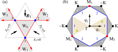
Figure 2: (a) Ternary phase diagram of strained graphene. The dashed triangle marks the boundary of the region in which all $x_{i}$’s are positive. In each region marked ${\rm W}_{i}$, there are two Weyl points in the Brillouin zone. In the other regions, the bands are characterized by nonzero winding numbers when traversed in the directions indicated by arrows. (b) The Brillouin zone with high symmetry points marked, including ${\bf K}=(4\pi/3a,0)$ (and equivalent points) and ${\bf M}_{1}=(0,2\pi/\sqrt{3}a)$. Dark gray (light tan) shaded regions indicate possible locations of Weyl points corresponding to region ${\rm W}_{0}$ (${\rm W}_{1})$, with white (yellow) disks showing generic possible arrangements. At each blue point $i$ ($=1,2,3$) in (a), there are zero modes along the pair of blue lines marked $i$ in (b). Along each red line in (a), there is a red point in (b) containing degenerate Weyl points.

Weyl points arise when $C({{\bm{q}}})=0$, which generically occurs for pairs of points $\pm{{\bm{q}}}^{*}$, where ${{\bm{q}}}^{*}$ is a solution of

$$C({\bm{q}}^{*})=x_{1}e^{i{{\bm{q}}}^{*}\cdot{{\bm{d}}}_{1}}+x_{2}e^{i{{\bm{q}}}^{*}\cdot{{\bm{d}}}_{2}}+x_{3}e^{i{{\bm{q}}}^{*}\cdot{{\bm{d}}}_{3}}=0.$$ (23)

When $x=(1/3,1/3,1/3)$ (at the middle of ${\rm W}_{0}$ in Fig. 2(a)) Eq. (23) is satisfied at the $\pm{\rm K}$ points ${\bm{q}}^{*}=\pm{\bm{q}}_{\rm K}$, where

$${\bm{q}}_{\rm K}={4\pi\over{3a}}{\hat{x}}\quad\Rightarrow\quad e^{i{\bm{q}}_{\rm K}\cdot{{\bm{d}}}_{j}}=e^{2\pi i(j-1)/3}.$$ (24)

This corresponds to the well known Weyl point at the Brillouin zone corner in unstrained graphene. In Fig. 3(a) we show the displacements of one of the zero frequency modes at ${\bm{q}}_{\rm K}$. It is straightforward to see in Fig. 3(a) that this is indeed a “floppy mode” in which, to linear order, each tri-bond undergoes a rigid rotation about its pivot point and hence is not stretched.

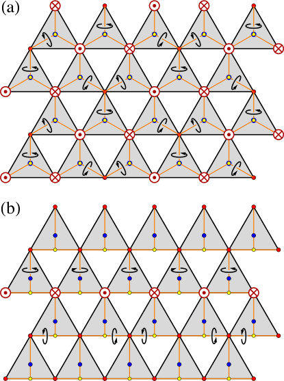
Figure 3: (a) A Weyl mode for $x=(1/3,1/3,1/3)$, corresponding to unstrained graphene. The pivot is at the centroid of the tri-bond. (b) A zero mode for $x=(0,1/2,1/2)$. The mode is confined to a single line. The pivot point is at the midpoint of the bottom edge, and each tri-bond rotates rigidly about its pivot so that vertices move in and out of the plane as indicated.

Because the phase of $C({\bm{q}})$ advances by $2\pi$ as ${\bm{q}}$ wraps around ${\bm{q}}^{*}$, the Weyl points are locally protected and cannot be removed by a smooth deformation. Therefore, there must be a Weyl phase in a finite region around $(1/3,1/3,1/3)$. However, it is also clear from (23) that for $x=(1,0,0)$, $(0,1,0)$ or $(0,0,1)$ there are no solutions to $C({\bm{q}}^{*})=0$. Thus, there must be a gapped phase in the vicinity of the three corners of the dashed triangle in Fig. 2(a).

To determine the phase boundaries, we note that Weyl points can only only disappear if they meet, which must occur at a time-reversal-invariant point ${{\bm{q}}}^{*}=-{{\bm{q}}}^{*}+{{\bm{G}}}$, where ${\bm{G}}$ is a reciprocal lattice vector. ${{\bm{q}}}^{*}=0$ is ruled out for finite $x$ because $C(0)=x_{1}+x_{2}+x_{3}=1$, so this must occur at one of the three M points

$${\bm{q}}_{{\rm M}j}={2\pi\over{\sqrt{3}a}}\hat{{\bm{d}}}_{j},$$ (25)

which satisfy

$${\bm{q}}_{{\rm M}j}\cdot{{\bm{d}}}_{k}=\left\{\begin{array}[]{ll}2\pi/3&j=k\\ -\pi/3&j\neq k\end{array}\right..$$ (26)

Then Eq. (23) requires

$$x_{k}-x_{k-1}-x_{k+1}=0$$ (27)

where the subscript is defined cyclically. Together with $\sum x_{i}=1$, this implies $x_{k}=1/2$ and $x_{k-1}+x_{k+1}=1/2$, which define the three red lines bounding the triangle inscribed in the dashed region of Fig. 2(a). The Weyl phase in the vicinity of $x=(1/3,1/3,1/3)$ thus corresponds to the region ${\rm W}_{0}$. On the boundary of ${\rm W}_{0}$ the Weyl points meet and annihilate.

The points outside the dashed triangle of Fig. 2(a) have the pivot outside the tri-bond and have one or two of the $x_{i}$ negative. This corresponds in the graphene model to having bond(s) with a negative hopping amplitude. Systems with negative hopping amplitudes are closely related to systems with positive hopping amplitudes. The sign of the hopping amplitude on one of the three bonds (say along ${\bf d}_{1}$) can be changed by a non-uniform gauge transformation that changes the signs of all sites on every other horizontal (zig-zag) line of bonds on the honeycomb lattice. This transformation takes bond hopping amplitudes $(t_{1},t_{2},t_{3})\rightarrow(-t_{1},t_{2},t_{3})$, which in our mechanical model takes $x=(x_{1},x_{2},x_{3})\rightarrow x^{\prime}=(-x_{1},x_{2},x_{3})/(x_{2}+x_{3}-x_{1})$. This gauge transformation does not change the normal mode frequencies except for an overall constant factor due to the relation between $x_{i}$ and $t_{i}$. However, since the gauge transformation is at a nonzero wavevector ${\bm{q}}_{{\rm M}1}$, it leads to a shift in the wavevector of the normal modes and hence a transformation of the dispersion relation:

$$\omega_{x^{\prime}}({\bm{q}})=(x_{2}+x_{3}-x_{1})^{-1}\omega_{x}({\bm{q}}+{\bm{q}}_{{\rm M}1}).$$ (28)

This transformation maps $x=(1/3,1/3,1/3)$ to $x^{\prime}=(-1,1,1)$, so the normal mode spectra at these two pivot point locations are related by Eq. (28). In particular, for $x^{\prime}$ there are Weyl points at ${\bm{q}}_{\rm K}+{\bm{q}}_{{\rm M}1}$. Indeed, Eq. (23) is satisfied for ${\bm{q}}^{*}=\pm{\bm{q}}_{\rm L}$, where

$${\bm{q}}_{\rm L}={2\pi\over{3a}}{\hat{x}}\quad\Rightarrow\quad e^{i{\bm{q}}_{\rm L}\cdot{{\bm{d}}}_{(1,2,3)}}=(e^{0},e^{\pi i/3},e^{-\pi i/3}).$$ (29)

It can be checked that ${\bm{q}}_{\rm L}=-{\bm{q}}_{\rm K}+{\bm{q}}_{{\rm M}1}$ up to a reciprocal lattice vector. More generally, the Weyl phase ${\rm W}_{0}$ maps to the region ${\rm W}_{1}$ in Fig. 2(a). Similar transformations identify the Weyl phases ${\rm W}_{2}$ and ${\rm W}_{3}$, whose boundaries are again given by the red lines defined by Eq. (27).

When $x$ is in ${\rm W}_{0}$ in Fig. 2(a), the Weyl points are at ${\pm{\bm{q}}}^{*}$, which reside in the dark gray regions of Fig. 2(b). When $x$ is in ${\rm W}_{1}$, the Weyl points are at ${\pm{\bm{q}}}^{*}$ residing in the light tan regions of Fig. 2(b), and there are symmetry related regions corresponding to ${\rm W}_{2}$ and ${\rm W}_{3}$. When a path through ${\rm W}_{0}$ is traversed, beginning on one edge and ending another, a pair of Weyl points created at ${\rm M}_{j}$ pass through the diametrically opposite dark gray regions of Fig. 2(b) and annihilate at ${\rm M}_{j\pm 1}$. Similarly, for a path that begins on right boundary of ${\rm W}_{1}$, passes through ${\rm W}_{1}$, and terminates on the left boundary, the Weyl points are born at $\pm{\rm M}_{2}$, pass through the opposite tan regions of Fig. 2(b), and annihilate at $\pm{\rm M}_{3}$. For $x=(-\alpha,(\alpha+1)/2,(\alpha+1)/2)$ with $\alpha\gg 1$, Weyl points occur at ${\bm{q}}^{*}\approx\pm(2\sqrt{2/\alpha}\,/a)\hat{x}$, converging to the $\Gamma$ point as $\alpha\rightarrow\infty$.

Outside the ${\rm W}_{n}$ regions there is a gap everywhere in the Brillouin zone. There are three disconnected phases that are topologically distinct. The topological polarization can be most easily evaluated at the three simple points (indexed by $j=1,2,3$) $x_{i}=\delta_{ij}$. Then,

$$C({\bm{q}})=e^{i{{\bm{q}}}\cdot{{\bm{d}}}_{j}}.$$ (30)

The topological polarization ${\bm{R}}_{T}$ is determined by the winding numbers $n_{i}$ of this phase over the independent cycles of the Brillouin zone:

$$n_{i}=-{1\over{2\pi i}}\oint_{C_{i}}C^{-1}dC=-{1\over{2\pi}}{\bm{b}}_{i}\cdot{\bm{d}}_{j}$$ (31)

where $C_{i}$ is the cycle along reciprocal lattice generator ${\bm{b}}_{i}$, which satisfies ${\bm{b}}_{i}\cdot{\bm{a}}_{j}=2\pi\delta_{ij}$ for Bravais lattice generators ${\bm{a}}_{j}$. (Note the minus sign in this equation, which appears because it is defined as an integral over $C({\bm{q}})$ rather than $Q({\bm{q}})$ as in KaneLub2014 .) Writing

$${\bm{R}}_{T}=n_{1}{\bm{a}}_{1}+n_{2}{\bm{a}}_{2}$$ (32)

then gives

$${\bm{R}}_{T}=-{\bm{d}}_{j},$$ (33)

which follows from the “completeness” relation $\sum_{i=1}^{2}{\bm{a}}_{i}{\bm{b}}_{i}=2\pi I$, where $I$ is the unit matrix. The value of ${\bm{R}}_{T}$ depends on the real-space positions assigned to the $A$ and $B$ lattice sites, i.e., on our gauge choice. In our current symmetric choice, in which the $B$ sites do not sit at a center of inversion, ${\bm{R}}_{T}$ is not a lattice vector, but the differences between of ${\bm{R}}_{T}$’s in different phases are. Arrows indicating ${\bf R}_{T}$ are indicated in Fig. 2(a). (In the gauge where the origin lies at an $A$ site, we subtract a particular ${\bm{d}}_{k}$ from each ${\bm{d}}_{j}$ in Eq. (30), and the $n_{i}$ are all 0 or $\pm 1$.)

Finally, we note that the line in the phase diagram corresponding to $x_{1}=0$ (where the pivot point is along the bottom edge of the tri-bond) corresponds to a one dimensional limit, in which the system consists of decoupled horizontal lines that are similar to the SSH model. In this case there is a direct transition between topologically distinct gapped phases, which occurs at the blue point $x=(0,1/2,1/2)$. Here

$$C({\bm{q}})=\cos(q_{x}a/2)e^{-iq_{y}a/(2\sqrt{3})},$$ (34)

so that there is a line of zero modes at $q_{x}=\pm\pi/a$ along the vertical line that connects ${\rm M}_{2}$ and ${\rm M}_{3}$, indicated by a blue line in Fig. 2(b). This situation is analogous to that in critical kagome lattices when there are parallel straight lines of bonds SunLub2012 . The zero modes are easy to visualize: as we have discussed, rotation of a tri-bond about any axis passing through its pivot point produces no stretch and costs no energy. Consider a horizontal line of edges containing the ${\bm{d}}_{2}$ and ${\bm{d}}_{3}$ vertices of the row of tri-bonds above it and the ${\bm{d}}_{1}$ vertex of the row of tri-bonds below it as shown in Fig. 3(b). Rotating neighboring tri-bonds in the upper row by $\delta\theta$ in opposite directions about the axis passing through the pivot point and ${\bm{d}}_{1}$ (the top vertex) while rotating neighboring tri-bonds in the lower row in opposite directions by $\delta\theta/\sqrt{3}$ about the axis along their bottom edges produces a zero mode. This operation only affects the given rows, and there is a zero mode for each line of bonds.

Associated with each zero mode, there must be a state of self stress. Alternating equal-amplitude stresses on tri-bonds along any row produces the desired zero-force state. In the case with $x_{1}=0$ and $x_{2}=x_{3}=1/2$, the stress tends to bend the tri-bonds symmetrically either upward or downward about a line passing through the pivot point and vertex 1. Alternation of the sign of the stresses causes vertices 2 and 3 to experience equal and opposite forces from the two tri-bonds each shares along the x axis. When $x_{2}\neq x_{3}$, neighboring rows are still decoupled, and each is equivalent to the SSH model, whose critical point occurs when $x_{2}=x_{3}$. Thus the lines defined by $x_{i}=0$ for some $i$, which include the perimeter of the region where all $x_{i}$ are positive, correspond to the 1D limit.

IV Edge States

Strips with periodic boundary conditions in one direction or samples with free sides on all boundaries can be produced by removing lines of tri-bonds from the system under full periodic boundary conditions. Each line of cut tri-bonds creates two free edges. Since the number of sites and tri-bonds are equal under periodic boundary conditions, the index theorem reduces to

$$N_{0}-S=\Delta N_{B}\qquad$$ (35)

where $\Delta N_{B}$ is the total number of tri-bonds cut to produce the free edges. A similar equation applies to each wavenumber $q$ along the cut producing a strip:

$$n_{0}(q)-s(q)=\Delta n_{B},$$ (36)

where $\Delta n_{B}$ is the number of bonds cut per unit cell of one of the exposed edges. How zero modes are distributed on the free edges depends on the topological polarization ${\bm{R}}_{T}$ and a local surface polarization ${\bm{R}}_{L}$ KaneLub2014 ; LubenskySun2015 according to the same formula derived for central-force Maxwell lattices. The number of zero modes per edge unit cell (or equivalently per edge wavenumber $q$) for a given edge corresponding to a lattice “plane” indexed by the reciprocal lattice vector ${\bm{G}}$ pointing along the edge’s outer normal is

$$n_{0}=({\bm{R}}_{T}+{\bm{R}}_{L})\cdot{\bm{G}}/(2\pi).$$ (37)

The local polarization ${\bm{R}}_{L}$ is simply the electric polarization at the given edge that arises from assigning a charge $+1$ to sites on the $A$-sublattice and a charge $-1$ to sites on the $B$ sublattice. Of course only components of ${\bm{R}}_{L}$ parallel to ${\bm{G}}$ contribute to $n_{0}$ so we are free to add arbitrary components to ${\bm{R}}_{L}$ parallel to the edge .

It is instructive to look at a couple of examples. Consider the strip with edges parallel to the $x$-axis as shown in Fig. 3(b). To produce this strip, one tri-bond per surface unit cell had to be removed, so there is a total of one zero mode per wavenumber on the two exposed edges. The local polarization ${\bm{R}}_{L}^{L}$ on the lower edge with outer surface normal, ${\bm{G}}=-4\pi/{\sqrt{3}a}\hat{y}$, is equally well represented by $-{\bm{d}}_{1}/2$ , ${\bm{d}}_{2}$, or ${\bm{d}}_{3}$, giving a local contribution to the number of edge zero modes of $1/3$. On the upper surface ${\bm{R}}_{L}^{U}=+{\bm{d}}_{1}$, for a contribution of $2/3$ to edge-mode count. The topological count for the bottom surface is respectively $2/3$, $-1/3$, and $-1/3$ for ${\bm{R}}_{T}$ equal to $-{\bm{d}}_{1}$, $-{\bm{d}}_{2}$, and $-{\bm{d}}_{3}$ for a total of one zero mode on the bottom surface and none on the top surface for ${\bm{R}}_{T}=-{\bm{d}}_{1}$ and no zero mode on the bottom and one the top surface for ${\bm{R}}_{T}=-{\bm{d}}_{2},-{\bm{d}}_{3}$. A similar analysis for a strip parallel to the $y$-axis yields for the number of zero modes on the left and right surfaces $(n_{0}^{R},n_{0}^{L})=(1,1)$, $(0,2)$, and $(2,0)$ for ${\bm{R}}_{T}$ equal to $-{\bm{d}}_{1}$, $-{\bm{d}}_{2}$, and $-{\bm{d}}_{3}$, respectively. When there are Weyl points, zero modes shift from one side of a strip to the other at edge wavenumbers equal to the projections of the wavenumber of the Weyl points onto the edge.

Insight into Eq. (37) can be gained by considering what happens to $C$ when the sites and tri-bonds are indexed at different positions (without changing the lattice itself). Let

$${\bm{R}}_{A}^{\prime}={\bm{R}}_{A}+\Delta{\bm{R}}_{A}\quad{\rm and}\quad{\bm{R}}_{B}^{\prime}={\bm{R}}_{B}+\Delta{\bm{R}}_{B},$$ (38)

and define the “gauge-transformed” compatibility matrix,

$$C^{\prime}({\bm{R}}_{A}^{\prime},{\bm{R}}_{B}^{\prime})=C({\bm{R}}_{A}^{\prime}-\Delta{\bm{R}}_{A},{\bm{R}}_{B}^{\prime}-\Delta{\bm{R}}_{B}).$$ (39)

Then

$$C^{\prime}({\bm{q}}) =e^{-i{\bm{q}}\cdot(\Delta{\bm{R}}_{A}-\Delta{\bm{R}}_{B})}C({\bm{q}})$$

$$|C({\bm{q}})|\,e^{-i{\bm{q}}\cdot(\Delta{\bm{R}}_{A}-\Delta{\bm{R}}_{B}+{\bm{R}}_{T})}.$$ (40)

Thus if we chose $\Delta{\bm{R}}_{A}-\Delta{\bm{R}}_{B}={\bm{R}}_{L}$, we find that the total polarization of $C^{\prime}({\bm{q}})$ is ${\bm{R}}^{\prime}={\bm{R}}_{L}+{\bm{R}}_{T}$ . Let ${\bm{q}}=(q_{\perp},q_{\parallel})$, where $q_{\perp}$ and $q_{\parallel}$ are, respectively, the components of ${\bm{q}}$ perpendicular (positive toward the sample interior) and parallel to the lattice plane in question, and define $\eta=\exp(iq_{\perp}a_{\perp})$, where $a_{\perp}$ is the depth of the surface unit cell, and $0<q_{\perp}\leq|{\bm{G}}|$, where ${\bm{G}}$ is the inner normal reciprocal lattice vector associated with the lattice plane. $C^{\prime}(\eta,q_{\parallel})$ contains only positive powers of $\eta$, and thus no poles in $\eta$, and as a result, the integral

$$n_{0}({\bm{G}})=\frac{1}{2\pi i}\oint d\eta\frac{d}{d\eta}\ln C^{\prime}(\eta,q_{\parallel})=\frac{{\bm{G}}\cdot({\bm{R}}_{L}+{\bm{R}}_{T})}{2\pi}$$ (41)

counts the number of zero modes at the surface determined by ${\bm{G}}$. As particular examples, consider the bottom and left edges in Fig. 1. In the first case, ${\bm{R}}_{L}=-{\bm{d}}_{1}/2$ and

$$C^{\prime}(\eta,q_{x})=x_{1}\eta+x_{2}e^{-iq_{x}a/2}+x_{3}e^{iq_{x}a/2},$$ (42)

where $\eta=\exp(iq_{y}\sqrt{3}\,a/2)$, has at most one zero and no poles, in agreement with our result that the top and bottom surfaces can have either one zero mode or none. In the second case, ${\bm{R}}_{L}={\bm{d}}_{2}$, and

$$C^{\prime}(\eta,q_{x})=x_{3}\eta^{2}+x_{1}\eta+x_{2}e^{iq_{y}\sqrt{3}\,a/2},$$ (43)

where $\eta=\exp(iq_{x}a/2)$. Again, there are no poles, but the highest power of ${\eta}$ is 2, and according to Eq. (41), there can be 0, 1, or 2 zero modes in agreement with our previous results.

When there are Weyl modes, the number of zero modes on a free edge of a strip will change when $q_{||}$ passes through the projection of a Weyl point onto that edge BurkovBal2011a ; RocklinLub2016 . The total number of zero modes does not change at this transition, so there must be a change of the opposite sign in the number of zero modes on the opposite edge. In other words, zero modes move from one side of the sample to the opposite at a projection of a Weyl point. A similar phenomenon occurs at domain walls in systems under periodic boundary conditions, in which the number of zero modes equals the number of states of self-stress and is given by

$$\nu_{T}={\bm{G}}\cdot({\bm{R}}_{T}^{1}-{\bm{R}}_{T}^{2})/2\pi,$$ (44)

where $\nu_{T}$ is equal to the number of zero modes per wavenumber if it is positive and minus the number of states of self stress if it is negative. Thus a change in the number of zero modes on a zero-mode domain wall, which occurs at $q_{\parallel}$ equal to the projected Weyl wavenumber, must be accompanied by an equal change in the number of Weyl states of self-stress on a self-stress domain wall.

V Physical Models

Physical realization of the mechanical graphene model poses some technical challenges, but some straightforward approaches are possible. The simplest version of the tri-bond uses a spring that directly measures the stretch. The tri-bond consists of a rigid plate suspended at its pivot point on a vertical spring that is attached to a rigid ceiling. The plates are connected at each vertex to a ball of mass $m$ through a mechanism that allows free rotations about the axes passing through the center of the ball and the pivot point on the plate. A possible design with three nested universal ball joints is shown in Fig. 4.

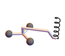
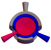
Figure 4: Left: Tri-bond “plate” with pivot at an arbitrary location. The bars are assumed to be rigid and have negligible mass compared to the balls. Right: Cutaway view of a three-pronged ball joint for connecting three plates to a single mass. The holes in the outer two spherical shells allow for rotations and twists of the each of the three arms about any axis through the common center of the spheres.

By attaching a lever arm to each plate that extends arbitrarily far from its centroid and attaching the spring to the end of it as shown in Fig. 4, the pivot point can be placed at any location in the plane, thus allowing the realization of the complete phase diagram of Fig. 2.

The height of the pivot point is precisely $\sum x_{i}z_{i}$, so the difference in energy in the spring (and gravity) from the equilibrium configuration in which all plates are horizontal is exactly the desired tri-bond energy. To mimic the spectrum of graphene, we need the kinetic energy matrix expressed in terms of the corner height variables $z({\bm{R}}_{A})$ to be a multiple of the identity: $E_{K}=(1/2)m\sum_{A}\dot{z}({\bm{R}}_{A})^{2}$. Thus we take the mass of a plate to be negligible compared to the mass of a corner ball. Note that the deviation from coplanarity of the plate corners and pivot point, which defines the tri-bond stretch, is measured with respect to the fixed equilibrium position of the pivot point rather than the pivot point that moves with the rigid plate (i.e., the position where the spring is attached).

In the limit of small deviations from equilibrium, this model directly mimics the generic discussion of the tri-bond above. Because the tri-bond stretch is directly encoded in a single spring and the height variables are literally encoded as heights of the ball joints, both ${\bm{e}}$ and ${\bm{z}}$ are immediately visible. For example, the self-stress state of the one-dimensional row of Fig. 3 is simply an alternating pattern of tension and compression in the springs along that row.

Other physical models could exhibit the mechanical graphene phase diagram, if not the exact same spectrum. All that is required is a potential energy of the form

$$U=\sum_{B}\frac{1}{2}k(x_{1},x_{2},x_{3})(x_{1}z_{1}+x_{2}z_{2}+x_{3}z_{3})^{2},$$ (45)

where the effective stiffness $k$ may depend on the location of the pivot. Because the features of greatest interest are zero modes, the form of the kinetic energy does not affect their existence or locations in the Brillouin zone, though it will affect the details of the spectrum at finite frequency if the kinetic energy is not simply a multiple of $\dot{z}_{1}^{2}+\dot{z}_{2}^{2}+\dot{z}_{3}^{2}$.

A natural example realizes the tri-bond energy as the bending energy of a triangular elastic plate that is pinned at the pivot point and attached at each vertex to two other plates. While the precise form of the lowest potential energy of the sheet for arbitrary (small) choices of the corner heights is difficult to calculate due to the boundary conditions at the corners and on the free edges, it must vanish for all rigid rotations of the plate, for which $x_{1}z_{1}+x_{2}z_{2}+x_{3}z_{3}=0$, and thus cannot depend on any other linear combination of the corner heights.

Another possibility consists of rigid plates coupled pairwise by springs at their corners. In this model, there are two degrees of freedom per plate (the two rocking angles) and thus two vibrational bands. One band is fully gapped, consisting of modes in which the net displacement of the three plate corners at any given $A$ site is zero. The other band exhibits the mechanical graphene phases, with each plate effectively acting as a tri-bond that couples the average displacements at each $A$ site.

VI Concluding remarks

This paper has introduced a mechanical model that is a precise analog of the tight-binding model of graphene, and defines an appropriate two dimensional generalization of the SSH analog introduced in Ref. KaneLub2014 . This model system exhibits a rich phase diagram of Weyl phases, along with gapped phases with distinct topological polarizations. Our proposed structures are amenable to physical implementation, and it will be interesting to construct them and to probe their mechanical mode structures.

In addition, our construction introduces the tri-bond, which opens a new avenue for studies of Maxwell lattices. It will be interesting to use this approach, and generalizations of it, to construct new classes of two and three dimensional mechanical systems.

- [1] N. Nakahara. Geometry, Topology and Physics. Institute of Physics Publishing, Bristol, 2nd edition, 2008. p. 79 and chapter 12.
- [2] G. E. Volovik. The Universe in a Helium Droplet. Clarenden, Oxford, 2003.
- [3] G.E. Volovik. Quantum phase transitions from topology in momentum space. Lecture Notes in Physics, 718:31 73, 2007.
- [4] W. P. Su, J. R. Schrieffer, and A. J. Heeger. Solitons in polyacetalene. Phys. Rev. Lett., 42:1698, 1979.
- [5] R. Jackiw and C. Rebbi. Solitons with fermion number 1/2. Phys. Rev. D, 13(12):3398–3409, 1976.
- [6] B. I. Halperin. Quantized hall conductance, current-carrying edge states, and the existence of extended states in a two-dimensional disordered potential. Phys. Rev. B, 25(4):2185–2190, 1982.
- [7] F. D. M. Haldane. Model for a quantum hall effect without landau levels - condensed matter realization of the parity anomaly. Phys. Rev. Lett., 61(18):2015–2018, 1988.
- [8] C. L. Kane and E. J. Mele. Z(2) topological order and the quantum spin Hall effect. Phys. Rev. Lett., 95(14):146802, 2005.
- [9] B. Andrei Bernevig, Taylor L. Hughes, and Shou-Cheng Zhang. Quantum spin Hall effect and topological phase transition in HgTe quantum wells. Science, 314(5806):1757–1761, 2006.
- [10] J. E. Moore and L. Balents. Topological invariants of time-reversal-invariant band structures. Phys. Rev. B, 75:121306, 2007.
- [11] Liang Fu, C. L. Kane, and E. J. Mele. Topological Insulators in Three Dimensions. Phys. Rev. Lett., 98:106803, 2007.
- [12] M. Z. Hasan and C. L. Kane. Colloquium : Topological insulators. Rev. Mod. Phys., 82:3045–3067, Nov 2010.
- [13] Xiao-Liang Qi and Shou-Cheng Zhang. Topological insulators and superconductors. Rev. Mod. Phys., 83(4):1057–1110, 2011.
- [14] C. L. Kane and T. C. Lubensky. Topological boundary modes in isostatic lattices. Nature Phys., 10(1):39–45, 2014.
- [15] T. C. Lubensky, C. L. Kane, Xiaoming Mao, A. Souslov, and Kai Sun. Phonons and elasticity in critically coordinated lattices. Reports on Progress in Physics, 78(7):073901, 2015.
- [16] Jayson Paulose, Bryan Gin-ge Chen, and Vincenzo Vitelli. Topological modes bound to dislocations in mechanical metamaterials. Nature Physics, 11(2):153–156, 2015.
- [17] J. Paulose, A. S. Meeussen, and V. Vitelli. Selective buckling via states of self-stress in topological metamaterials. Proceedings of the National Academy of Sciences of the United States of America, 112(25):7639–7644, 2015.
- [18] Bryan Gin-ge Chen, Nitin Upadhyaya, and Vincenzo Vitelli. Nonlinear conduction via solitons in a topological mechanical insulator. Proceedings of the National Academy of Sciences of the United States of America, 111(36):13004–13009, 2014.
- [19] Vincenzo Vitelli, Nitin Upadhyaya, and Bryan Gin-ge Chen. Topological mechanisms and classical spinor fields. arXiv:1407.2890, 2014.
- [20] Bryan Gin-ge Chen, Bin Liu, Arthur A. Evans, Jayson Paulose, Itai Cohen, Vincenzo Vitelli, and C. D. Santangelo. Topological mechanics of origami and kirigami. Phys. Rev. Lett., 116:135501, 2016.
- [21] Meng Xiao, Guancong Ma, Zhiyu Yang, Ping Sheng, Z. Q. Zhang, and C. T. Chan. Geometric phase and band inversion in periodic acoustic systems. Nature Physics, 11(February), 2015.
- [22] Hoi Chun Po, Yasaman Bahri, and Ashvin Vishwanath. Phonon analog of topological nodal semimetals. Phys. Rev. B, 93:205158, 2016.
- [23] Zhaoju Yang, Fei Gao, Xihang Shi, Xiao Lin, Zhen Gao, Yidong Chong, and Baile Zhang. Topological Acoustics. Physical Review Letters, 114(11):1–4, 2015.
- [24] Lisa M. Nash, Dustin Kleckner, Alismari Read, Vincenzo Vitelli, Ari M. Turner, and William T. M. Irvine. Topological mechanics of gyroscopic metamaterials. Proceedings of the National Academy of Sciences, 112(47):14495–14500, 2015.
- [25] Pai Wang, Ling Lu, and Katia Bertoldi. Topological phononic crystals with one-way elastic edge waves. Phys. Rev. Lett., 115:104302, 2015.
- [26] Yao-Ting Wang, Pi-Gang Luan, and Shuang Zhang. Coriolis force induced topological order for classical mechanical vibrations. New Journal of Physics, 17(7):073031, 2015.
- [27] Roman Susstrunk and Sebastian D. Huber. Observation of phononic helical edge states in a mechanical topological insulator. Science, 349(6243):47–50, 2015.
- [28] Toshikaze Kariyado and Yasuhiro Hatsugai. Manipulation of dirac cones in mechanical graphene. Scientific Reports, 5:18107 EP, 2015.
- [29] V. Peano, C. Brendel, M. Schmidt, and F. Marquardt. Topological Phases of Sound and Light. Phys. Rev. X, 5:031011, 2015.
- [30] S. Hossein Mousavi, Alexander B. Khanikaev, and Zheng Wang. Topologically protected elastic waves in phononic metamaterials. Nature Communications, 6:8682 EP, 2015.
- [31] Alexander B. Khanikaev, Romain Fleury, S. Hossein Mousavi, and Andrea Alù. Topologically robust sound propagation in an angular-momentum-biased graphene-like resonator lattice. Nat. Comm., 6(8260), 2015.
- [32] D. Z. Rocklin, B. G. G. Chen, M. Falk, V. Vitelli, and T. C. Lubensky. Mechanical weyl modes in topological maxwell lattices. Physical Review Letters, 116(13):135503, 2016.
- [33] Yujie Zhou, Bryan Gin-ge Chen, Nitin Upadhyaya, and Vincenzo Vitelli. Kink-antikink asymmetry and impurity interactions in topological mechanical chains. Arxiv, 1608.02127, 2016.
- [34] C. L. Kane and E. J. Mele. Size, shape, and low energy electronic structure of carbon nanotubes. Phys. Rev. Lett., 78:1932–1935, 1997.
- [35] A. Kitaev. Anyons in an exactly solved model and beyond. Annals of Physics, 321:2–111, 2006.
- [36] C. R. Calladine. Buckminster Fuller “tensegrity” structures and Clerk Maxwell rules for the construction of stiff frames. Int. J. Solids Struct., 14(2):161–172, 1978.
- [37] Mahito Kohmoto and Yasumasa Hasegawa. Zero modes and edge states of the honeycomb lattice. Phys. Rev. B, 76:205402, 2007.
- [38] Kai Sun, Anton Souslov, Xiaoming Mao, and T. C. Lubensky. Surface phonons, elastic response, and conformal invariance in twisted kagome lattices. PNAS, 109(31):12369–12374, 2012.
- [39] A. A. Burkov and L. Balents. Weyl semimetal in a topological insulator multilayer. Physical Review Letters, 107(12):127205, 2011.