Real-time broadening of non-equilibrium density profiles and
the role of the specific initial-state realization
Abstract
The real-time broadening of density profiles starting from non-equilibrium states is at the center of transport in condensed-matter systems and dynamics in ultracold atomic gases. Initial profiles close to equilibrium are expected to evolve according to linear response, e.g., as given by the current correlator evaluated exactly at equilibrium. Significantly off equilibrium, linear response is expected to break down and even a description in terms of canonical ensembles is questionable. We unveil that single pure states with density profiles of maximum amplitude yield a broadening in perfect agreement with linear response, if the structure of these states involves randomness in terms of decoherent off-diagonal density-matrix elements. While these states allow for spin diffusion in the XXZ spin- chain at large exchange anisotropies, coherences yield entirely different behavior.
pacs:
05.60.Gg, 71.27.+a, 75.10.JmI Introduction
The mere existence of equilibration and thermalization is a key issue in many areas of modern many-body physics. While this question has a long and fertile history, it has experienced an upsurge of interest in recent years eisert2015 due to the advent of cold atomic gases langen2015 as well as due to the discovery of new states of matter such as many-body localized phases nandkishore2015 . In particular, the theoretical understanding has seen substantial progress by the fascinating concepts of eigenstate thermalization deutsch1991 ; srednicki1994 ; rigol2008 and typicality of pure quantum states gemmer2003 ; goldstein2006 ; popescu2006 ; reimann2007 ; bartsch2009 ; sugiura2012 ; sugiura2013 ; elsayed2013 as well as by the invention of powerful numerical methods such as density-matrix renormalization group schollwoeck2005 . Much less is known on the route to equilibrium as such reimann2016 and still the derivation of the conventional laws of (exponential) relaxation and (diffusive) transport on the basis of truly microscopic principles is a challenge to theory buchanan2005 .
In strictly isolated systems any coupling to heat baths or particle reservoirs and any driving by external forces is absent. In such systems, the only possibility to induce a non-equilibrium process is the preparation of a proper initial state. While different ways of preparation can be chosen, a sudden quench of the Hamiltonian is a common preparation scheme essler2016 . However, once a specific state is selected, a crucial question is: To what extent is this state a non-equilibrium state? To answer this question, it is natural to measure the observable one is interested in. If the expectation value is far from equilibrium, the state should be also. If this value is close to equilibrium, the state should be correspondingly. Moreover, only in the latter case, the resulting dynamics of the expectation value and linear response theory are expected to agree with each other. While this line of reasoning is certainly intuitive, it neglects internal degrees of freedom of the initial state. In particular, the measurement of a single observable cannot detect if the underlying state is pure or mixed, entangled or non-entangled, etc. Therefore, an intriguing question is: Do such internal details play any role for the dynamics of an expectation value?
In this paper, we investigate exactly this question for the anisotropic spin- Heisenberg chain. Dynamics in this integrable many-body model has been under active scrutiny in various theoretical works and, in particular, spin dynamics constitutes a demanding problem resolved only partially despite much effort shastry1990 ; narozhny1998 ; zotos1999 ; benz2005 ; heidrichmeisner2003 ; fujimoto2003 ; prosen2011 ; prosen2013 ; herbrych2011 ; karrasch2012 ; karrasch2013 ; steinigeweg2014-1 ; steinigeweg2015 ; carmelo2015 ; gobert2005 ; sirker2009 ; grossjohann2010 ; prelovsek2004 ; znidaric2011 ; steinigeweg2011 ; karrasch2014 ; steinigeweg2012 , even within the linear response regime and at high temperatures. While it has become clear that quasi-local conservation laws prosen2011 ; prosen2013 necessarily lead to ballistic behavior below the isotropic point, numerical studies prelovsek2004 ; znidaric2011 ; karrasch2014 ; steinigeweg2011 have reported signatures of diffusion above this point, in agreement with perturbation theory steinigeweg2011 and classical simulations steinigeweg2012 .
To investigate spin transport, we first introduce a class of pure initial states. These initial states feature identical density profiles, where a maximum peak is located in the middle of the chain and lies on top of a homogeneous background, similar to karrasch2014 . For a subclass with internal randomness we then show analytically that the resulting non-equilibrium dynamics can be related to equilibrium correlation functions via the concept of typicality. This relation is verified in addition by large-scale numerical simulations. These numerical simulations also unveil the existence of remarkably clean diffusion for large exchange anisotropies, as one of our central findings. Eventually, we demonstrate that entirely different behavior emerges without any randomness in the initial state.
II Model and Observables
The Hamiltonian of the XXZ spin- chain with periodic boundary conditions reads
| (1) |
where are spin- operators at site , is the number of sites, is the antiferromagnetic exchange coupling constant, and is the anisotropy. For all parameters, this model is integrable in terms of the Bethe Ansatz and the total magnetization is a strictly conserved quantity. We take into account all subsectors of , i.e., we consider the case . We note that, via the Jordan-Wigner transformation, this model can be mapped onto a chain of spinless fermions with particle interactions of strength and total particle number , i.e., (see Appendix A for the half-filling case ).
We are interested in the non-equilibrium dynamics of the local occupation numbers . Specifically, we consider the expectation values for the density matrix at time . In this way, we study the time-dependent broadening of density profiles for a given initial state . In this paper, we focus on pure states .
III Initial States
Obviously, it is possible to choose many different initial states and the resulting dynamics can depend on details of the specific choice. A frequently used preparation scheme is a quantum quench, i.e., is the eigenstate of another Hamiltonian. In this paper, however, we proceed in a different way.
To introduce our class of initial states, let be the common eigenbasis of all , i.e., the Ising basis. Then, this class reads
| (2) |
where are complex coefficients and projects onto Ising states with a particle in the middle of the chain. By construction, is maximum.
In the above class, a particular state is the one where all are the same. It yields and still . Hence, its density profile has a peak on top of a homogeneous background. However, exactly this density profile also results when the are drawn at random according to the unitary invariant Haar measure bartsch2009 (where real and imaginary part of the are drawn from a Gaussian distribution with zero mean, as done in our numerical simulations perfomed below). In other words, it is impossible to distinguish the two states with equal and random coefficients by a measurement of their initial density profiles note . Only at times , their density profiles can be different, if these density profiles differ at all. Note that similar have been studied in Ref. karrasch2014 .
Because our initial states are pure and have maximum as well, these states have to be considered as far-from-equilibrium states. Thus, it is natural to expect that the resulting dynamics of cannot be described by linear response theory. However, such a expectation turns out to be wrong for the case of random . In this case, is a typical state gemmer2003 ; goldstein2006 ; popescu2006 ; reimann2007 ; bartsch2009 ; sugiura2012 ; sugiura2013 ; elsayed2013 , i.e., a trace can be approximated by the expectation value with high accuracy in large Hilbert spaces. Using this fact and exact math (see Appendix B for more details), we find the relation
| (3) |
where . This relation is a first main result of our paper. It unveils that the expectation value of a far-from-equilibrium state is directly connected to a equilibrium correlation function. It is important to note that such a relation cannot be derived for the other case of equal (see also Appendix C for the specific type of randomness).
Due to the above relation, it is also possible to connect our non-equilibrium dynamics to the Kubo formula. To this end, one has to define the spatial variance
| (4) |
with and . Then, following Ref. steinigeweg2009 , it is straightforward to show that the time derivative of this variance
| (5) |
is given by the time-dependent diffusion coefficient
| (6) |
where is the well-known spin current. For , leads to such that scales ballistically. The partial conservation of for shastry1990 ; narozhny1998 ; zotos1999 ; benz2005 ; heidrichmeisner2003 ; fujimoto2003 ; prosen2011 ; prosen2013 ; herbrych2011 ; karrasch2012 ; karrasch2013 ; steinigeweg2014-1 ; steinigeweg2015 also excludes diffusive scaling in this regime. In fact, signatures of diffusion at high temperatures have been found only in the regime of large anisotropies prelovsek2004 ; znidaric2011 ; steinigeweg2011 ; karrasch2014 . Note that is merely a necessary and no sufficient criterion for diffusion since, by definition, the variance yields no information beyond the width of the distribution . This is why we study the full space dependence. For a recent numerical survey of Eq. (5), see karrasch2016 .
IV Numerical Method and Results
Numerically, the time evolution of a pure state can be calculated by the method of full exact diagonalization. But this method is restricted to sites, even if symmetries such as the translation invariance of are taken into account. Thus, we proceed differently and rely on a forward propagation of in real time. Such a propagation can be done by the use of fourth-order Runge-Kutta steinigeweg2014-1 ; steinigeweg2015 ; elsayed2013 or more sophisticated schemes such as Trotter decompositions or Chebyshev polynomials steinigeweg2014-2 ; jin2015 . Here, we use a massively parallelized implementation of a Chebyshev-polynomial algorithm. In this way, we can treat system sizes as large as . For such , we can guarantee that the initial peak is located sufficiently far from the boundary of the chain. Otherwise, we would have to deal with trivial finite-size effects and also Eq. (5) would not hold steinigeweg2009 .
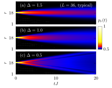
Next, we turn to our numerical results, starting with a typical initial state , i.e., the case of random . For a single realization of this state, we summarize in Fig. 1 the resulting expectation value in a 2D time-space density plot for different anisotropies , , and a large system with sites. Several comments are in order. First, for all values of shown, the initial peak monotonously broadens as a function of time and the non-equilibrium density profiles have the irreversible tendency to equilibrate. Such equilibration is non-trivial in view of our isolated and integrable model. Second, for times below the maximum depicted, the spatial extension of the density profiles is still smaller than the length of the chain. Thus, unwanted boundary effects do not emerge for such times. Third, the broadening of the density profiles is faster for smaller values of because the scattering due to particle interactions decreases as decreases. Moreover, for the small in Fig. 1 (c), the width of the density profile clearly increases linearly as a function of time. This linear increase is the expected ballistic dynamics arising from partial conservation of the spin current. In contrast, for the larger and in Figs. 1 (a) and (b), the width of the density profiles does not increase linearly and is rather reminiscent of a square-root behavior. However, such a conclusion is not possible on the basis of a density plot.
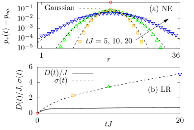
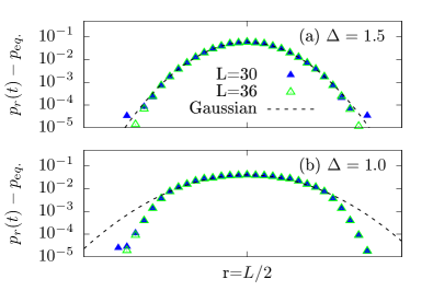
To gain insight into the dynamics at , we depict in Fig. 2 (a) the site dependence of the expectation values at fixed times , , and . Conveniently, we subtract the equilibrium value and use a semi-log plot to visualize also the tails of the density profiles. As illustrated by fits, the site dependence can be described by Gaussians (with as the only fit parameter)
| (7) |
and, remarkably, over several orders of magnitude. Such a pronounced Gaussian form of the density profiles is a second main result of our paper and has, to best of our knowledge, not been reported in the literature yet. This result unveils that the standard deviation is not just a width but also the only parameter required to describe the full site dependence. Furthermore, the Gaussian form is one of the clearest signatures of diffusion so far. Still, diffusion requires that scales as .
To further judge on diffusion, we show in Fig. 2 (b) the standard deviation , as resulting from the Gaussian fits in Fig. 2 (a). We further depict linear-response results for in Eq. (5) and the underlying in Eq. (6), as calculated in Ref. steinigeweg2015 for . On the one hand, the excellent agreement shows the very high accuracy of the typicality relation in Eq. (3). On the other hand, this agreement demonstrates that the known linear-response result , resulting from at such steinigeweg2011 ; steinigeweg2015 ; karrasch2014 , also holds for our non-equilibrium density dynamics. Hence, together with the Gaussian form, we can conclude that diffusion exists.

An analogous analysis for the isotropic point in Fig. 3 (a) shows that simple Gaussians are not able to describe the tails of the density profiles accurately. This is why the standard deviation of corresponding fits slightly deviates from the linear-response result in Fig. 3 (b). But these deviations disappear if is calculated exactly according to Eq. (4). Most notably, however, the time dependence of is inconsistent with diffusion, as can be seen easiest from the non-constant . In fact, points to superdiffusion znidaric2011 ; steinigeweg2012 , contrary to khait2016 .
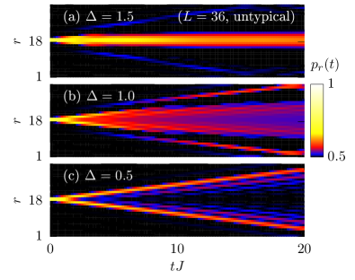
Now, we turn to the untypical initial state , i.e., the case of equal . Recall that for this state we obtain the same initial density profile but the relations in Eqs. (3) and (5) do not need to hold. In Fig. 4 we summarize the resulting expectation values in a 2D time-space density plot again. Compared to Fig. 1, the broadening turns out to be clearly different. The dynamics is frozen for in Fig. 4 (a) and features pronounced jets for in Fig. 4 (c). In particular, we do not find obvious indications of equilibration, at least for all times considered. These observations constitute a third main result of our paper. This result suggests that the lack of internal randomness in the initial condition is essential for the observation of non-equilibrium dynamics beyond linear response theory.
Finally, let us briefly mention another property of the untypical initial state , which could be responsible for the special dynamics found. This property is the lack of entanglement. In fact, it is easy to see that can be written as the product state
| (8) |
with a spin-up state in the middle of the chain and a spin-up/spin-down superposition at all other sites. By definition, such a product state is not entangled at all. In clear contrast, the typical initial state cannot be written as a product state.
V Conclusions
In this paper, we have investigated the real-time broadening of non-equilibrium density profiles in the spin- XXZ chain. First, we have introduced a class of pure initial states with identical density profiles where a maximum peak is located in the middle of the chain. Then, we have shown for a subclass with internal randomness that the resulting non-equilibrium dynamics can be connected to equilibrium correlation functions via the concept of typicality. This analytical result has been also verified by large-scale numerical simulations. These numerical simulations have further unveiled the existence of diffusion for large exchange anisotropies, as one of our key results. Finally, we have demonstrated that entirely different behavior emerges without any randomness in the initial state. Promising future directions of research include the identification of typical and untypical initial states in non-integrable models, in many-body localized phases, and at low temperatures as well as a systematic analysis of the role of entanglement.
Acknowledgments
We sincerely thank T. Prosen and F. Heidrich-Meisner for fruitful discussions. In addition, we gratefully acknowledge the computing time, granted by the “JARA-HPC Vergabegremium” and provided on the “JARA-HPC Partition” part of the supercomputer “JUQUEEN” stephan2015 at Forschungszentrum Jülich.
Appendix A Half-Filling Sector
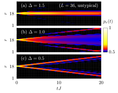
To demonstrate that our results do not depend on our specific choice of , we do the calculation in, e.g., Fig. 4 again for the half-filling sector . We depict the corresponding results in Fig. 5. It is clearly visible that the real-time broadening of the expectation values is practically the same, apart from minor details related to in the half-filling case.
Appendix B Typicality Approximation
Here, we provide details on the calculation leading to the relation in Eq. (3) of the main text. By carrying out the multiplication of the two brackets in the correlation function
| (9) |
and applying , we obtain
| (10) |
Using and a cyclic permutation in the trace, we get
| (11) |
Exploiting typicality of the pure state , the correlation function can be rewritten as
| (12) |
with the small error . Due to , this expression becomes
| (13) |
and, due to , it reads
| (14) |
where we have moved in addition the factor from the front to the denominator. Finally, due to the definition of , we can write
| (15) |
Therefore, comparing Eqs. (9) and (15) and skipping the small error for clarity yields
| (16) |
Appendix C Specific Type of Randomness
As stated in the main text, the relations in Eqs. (3) and (5) have to be understood for typical states drawn at random according to the unitary invariant Haar measure (where real and imaginary part of the are drawn from a Gaussian distribution with zero mean). However, it is instructive to consider other types of randomness. Thus, we choose
| (17) |
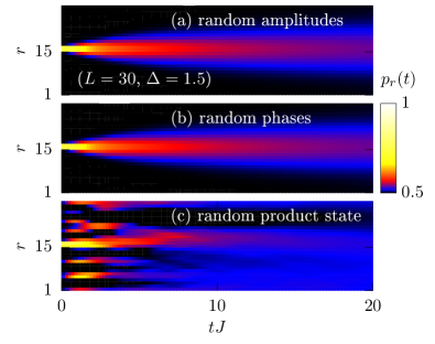
with constant amplitudes and random phases drawn from a uniform distribution . In Fig. 6 (a) and (b) we compare the resulting real-time broadening of the expectation values for this and the previous choice of the , where we focus on a single anisotropy and restrict ourselves to a chain length to reduce computational effort. The excellent agreement demonstrates that the specific type of randomness does not matter. Moreover, constant amplitudes as such are not responsible for the untypical dynamics observed in Fig. 4.
Note that not any kind of randomness can yield the same dynamical behavior. To illustrate this fact, let us randomize the product state in Eq. (8) of the main text in the following way: At all sites we replace the spin-up/spin-down superposition by
| (18) |
with site-dependent phases , drawn from a uniform distribution . This randomized product state has still and . It involves only random numbers, in contrast to the state from the Haar measure with random numbers. In Fig. 6 (c) we depict the resulting dynamics of the expectation values . Compared to the two other random cases in Figs. 6 (a) and (b), the dynamical behavior turns out to be very different. This difference suggests again that the lack of entanglement could be the source of untypical dynamics.
Appendix D Finite-Size Effects
Eventually, we show that our numerical results for the real-time broadening of the expectation values are free of significant finite-size effects. To this end, we redo the calculations in Figs. 2 (a) and 3 (a) for a smaller but still large system size . In Fig. 7 we depict the results of these calculations, together with the previous data. It is clearly visible that finite-size effects are negligibly small and are not responsible for the non-Gaussian tails at the isotropic point .
References
- (1) J. Eisert, M. Friesdorf, and C. Gogolin, Nature Phys. 11, 124 (2015).
- (2) T. Langen, R. Geiger, and J. Schmiedmayer, Annu. Rev. Condens. Matter Phys. 6, 201 (2015).
- (3) R. Nandkishore and D. A. Huse, Annu. Rev. Condens. Matter Phys. 6, 15 (2015).
- (4) J. M. Deutsch, Phys. Rev. A 43, 2046 (1991).
- (5) M. Srednicki, Phys. Rev. E 50, 888 (1994).
- (6) M. Rigol, V. Dunjko, and M. Olshanii, Nature 452, 854 (2008).
- (7) J. Gemmer and G. Mahler, Eur. Phys. J. B 31, 249 (2003).
- (8) S. Goldstein, J. L. Lebowitz, R. Tumulka, and N. Zanghì, Phys. Rev. Lett. 96, 050403 (2006).
- (9) S. Popescu, A. J. Short, and A. Winter, Nature Phys. 2, 754 (2006).
- (10) P. Reimann, Phys. Rev. Lett. 99, 160404 (2007).
- (11) C. Bartsch and J. Gemmer, Phys. Rev. Lett. 102, 110403 (2009); EPL (Europhys. Lett.) 96, 60008 (2011).
- (12) S. Sugiura and A. Shimizu, Phys. Rev. Lett. 108, 240401 (2012).
- (13) S. Sugiura and A. Shimizu, Phys. Rev. Lett. 111, 010401 (2013).
- (14) T. A. Elsayed and B. V. Fine, Phys. Rev. Lett. 110, 070404 (2013).
- (15) U. Schollwöck, Rev. Mod. Phys. 77, 259 (2005); Ann. Phys. 326, 96 (2011).
- (16) P. Reimann, Nature Commun. 7, 10821 (2016).
- (17) M. Buchanan, Nature Phys. 1, 71 (2005).
- (18) F. H. L. Essler and M. Fagotti, J. Stat. Mech. Theor. Exp., 064002 (2016).
- (19) B. S. Shastry and B. Sutherland, Phys. Rev. Lett. 65, 243 (1990).
- (20) B. N. Narozhny, A. J. Millis, and N. Andrei, Phys. Rev. B 58, 2921R (1998).
- (21) X. Zotos, Phys. Rev. Lett. 82, 1764 (1999).
- (22) J. Benz, T. Fukui, A. Klümper, and C. Scheeren, J. Phys. Soc. Jpn. 74, 181 (2005).
- (23) F. Heidrich-Meisner, A. Honecker, D. C. Cabra, and W. Brenig, Phys. Rev. B 68, 134436 (2003).
- (24) S. Fujimoto and N. Kawakami, Phys. Rev. Lett. 90, 197202 (2003).
- (25) T. Prosen, Phys. Rev. Lett. 106, 217206 (2011).
- (26) T. Prosen and E. Ilievski, Phys. Rev. Lett. 111, 057203 (2013).
- (27) J. Herbrych, P. Prelovšek, and X. Zotos, Phys. Rev. B 84, 155125 (2011).
- (28) C. Karrasch, J. H. Bardarson, and J. E. Moore, Phys. Rev. Lett. 108, 227206 (2012).
- (29) C. Karrasch, J. Hauschild, S. Langer, and F. Heidrich-Meisner, Phys. Rev. B 87, 245128 (2013).
- (30) R. Steinigeweg, J. Gemmer, and W. Brenig, Phys. Rev. Lett. 112, 120601 (2014).
- (31) R. Steinigeweg, J. Gemmer, and W. Brenig, Phys. Rev. B 91, 104404 (2015).
- (32) J. M. P. Carmelo, T. Prosen, and D. K. Campbell, Phys. Rev. B 92, 165133 (2015).
- (33) D. Gobert, C. Kollath, U. Schollwöck, and G. Schütz, Phys. Rev. E 71, 036102 (2005).
- (34) J. Sirker, R. G. Pereira, and I. Affleck, Phys. Rev. Lett. 103, 216602 (2009); Phys. Rev. B 83, 035115 (2011).
- (35) S. Grossjohann and W. Brenig, Phys. Rev. B 81, 012404 (2010).
- (36) P. Prelovšek, S. El Shawish, X. Zotos, and M. Long, Phys. Rev. B 70, 205129 (2004).
- (37) M. Žnidarič, Phys. Rev. Lett. 106, 220601 (2011).
- (38) C. Karrasch, J. E. Moore, and F. Heidrich-Meisner, Phys. Rev. B 89, 075139 (2014).
- (39) R. Steinigeweg and W. Brenig, Phys. Rev. Lett. 107, 250602 (2011).
- (40) R. Steinigeweg, EPL (Europhys. Lett.) 97, 67001 (2012).
- (41) Strictly speaking, by drawing at random, it is possible to get the outcome for all .
- (42) R. Steinigeweg, H. Wichterich, and J. Gemmer, EPL (Europhys. Lett.) 88, 10004 (2009).
- (43) R. Steinigeweg, F. Heidrich-Meisner, J. Gemmer, K. Michielsen, and H. De Raedt, Phys. Rev. B 90, 094417 (2014).
- (44) F. Jin, R. Steinigeweg, F. Heidrich-Meisner, K. Michielsen, and H. De Raedt, Phys. Rev. B 92, 205103 (2015).
- (45) C. Karrasch, T. Prosen, and F. Heidrich-Meisner, arXiv:1611.04832 (2016).
- (46) I. Khait, S. Gazit, N. Y. Yao, and A. Auerbach, Phys. Rev. B 93, 224205 (2016).
- (47) M. Stephan and J. Docter, J. Large-Scale Res. Facil. A1, 1 (2015).