Constraints on the trilinear Higgs coupling
from vector boson fusion and associated
Higgs production at the LHC

Abstract

We examine the constraints on the trilinear Higgs coupling $\lambda$ that originate from associated ($Vh$) and vector boson fusion (VBF) Higgs production in $pp$ collisions in the context of the Standard Model effective field theory. The 1-loop contributions to $pp\to Vh$ and $pp\to jjh$ that stem from insertions of the dimension-6 operator $O_{6}=-\lambda\left(H^{\dagger}H\right)^{3}$ are calculated and combined with the ${\cal O}(\lambda)$ corrections to the partial decay widths of the Higgs boson. Employing next-to-next-to-leading order QCD predictions, we analyse the sensitivity of current and forthcoming measurements of the signal strengths in $Vh$ and VBF Higgs production to changes in $\lambda$. We show that future LHC runs may be able to probe modifications of $\lambda$ with a sensitivity similar to the one that is expected to arise from determinations of double-Higgs production. The sensitivity of differential $Vh$ and VBF Higgs distributions to a modified $h^{3}$ coupling is also studied.

1 Introduction

Within the Standard Model (SM), the mass and the self-interactions of the Higgs field $h$ are parametrised by the potential

$${\cal L}_{\rm SM}\supset-V_{\rm SM}=-\frac{m_{h}^{2}}{2}\hskip 1.42262pth^{2}-\lambda v\hskip 0.7113pth^{3}-\frac{\kappa}{4}\hskip 1.42262pth^{4}\,,$$ (1)

where $v=246.22\,{\rm GeV}$ denotes the Higgs vacuum expectation value and

$$\lambda=\kappa=\frac{m_{h}^{2}}{2v^{2}}\,.$$ (2)

The LHC measurement of the Higgs-boson mass $m_{h}=125.09\,{\rm GeV}$ ATLASCMS determined the first term in (1), but the $h^{3}$ and $h^{4}$ couplings, and in particular the SM relation (2) have not been tested. Trying to constrain the Higgs self-couplings and thereby exploring the mechanism of electroweak symmetry breaking (EWSB) is hence an important goal of forthcoming LHC runs and other future high-energy colliders such as a hadron-hadron Future Circular Collider or a Circular Electron-Positron Collider.

One way to constrain the coefficients $\lambda$ and $\kappa$ in (1) consists in measuring double-Higgs and triple-Higgs production. Since the cross section for $pp\to 3h$ production is of ${\cal O}(0.1\,{\rm fb})$ at $14\,{\rm TeV}$ centre-of-mass energy ($\sqrt{s}$) even the high-luminosity option of the LHC (HL-LHC) will only be able to set very loose bounds on the Higgs quartic. The prospect to observe double-Higgs production at the HL-LHC is considerably better because at $14\,{\rm TeV}$ the $pp\to hh$ production cross section amounts to ${\cal O}(35\,{\rm fb})$ Glover:1987nx ; Plehn:1996wb ; Dawson:1998py ; Djouadi:1999rca ; deFlorian:2013jea ; Grigo:2013rya ; Borowka:2016ehy ; Borowka:2016ypz . Measuring double-Higgs production at the HL-LHC however still remains challenging (see for instance Baur:2002qd ; Baur:2003gp ; Dolan:2012rv ; Baglio:2012np ; Barr:2013tda ; Dolan:2013rja ; Papaefstathiou:2012qe ; Goertz:2013kp ; Maierhofer:2013sha ; deLima:2014dta ; Englert:2014uqa ; Liu:2014rva ; Goertz:2014qta ; ATL-PHYS-PUB-2014-019 ; Azatov:2015oxa ; Dall'Osso:2015aia ; ATL-PHYS-PUB-2015-046 ; Kling:2016lay ) and as a result even with the full data set of $3\,{\rm ab}^{-1}$ only an ${\cal O}(1)$ determination of the trilinear Higgs coupling seems possible under optimistic assumptions.

A second possibility consists in studying the effects that a modification of $\lambda$ has at loop level in single-Higgs production. In fact, such indirect probes of the $h^{3}$ coupling have been first proposed in the context precision studies of $e^{+}e^{-}\to hZ$ McCullough:2013rea ; Shen:2015pha and subsequently extended to observables accessible at hadronic machines such as the LHC Gorbahn:2016uoy ; Degrassi:2016wml . For both types of colliders it has been shown that future determination of $\lambda$ via loop effects are complementary to the direct HL-LHC determination through $pp\to hh$, since these probes can provide competitive constraints under the simplified assumption that new-physics effects dominantly modify the $h^{3}$ coupling.

This paper is a sequel to the article Gorbahn:2016uoy , in which two of us have calculated the ${\cal O}(\lambda)$ corrections to the $gg\to h$ and $h\to\gamma\gamma$ processes that arise at the 2-loop level within the SM effective field theory (SMEFT). The discussion in the present paper focuses instead on associated ($Vh$) and vector boson fusion (VBF) Higgs production. Specifically, we compute the 1-loop contributions to the $pp\to Vh$ and $pp\to jjh$ amplitudes that result from insertions of the effective operator $O_{6}=-\lambda\left(H^{\dagger}H\right)^{3}$. Combining these contributions with the ${\cal O}(\lambda)$ corrections to the partial decay widths of the Higgs boson, we analyse the sensitivity of present and future LHC measurements of the $Vh$ and VBF Higgs processes to shifts in the trilinear Higgs interactions. In order to obtain high-precision predictions for the $Vh$ and VBF Higgs cross sections we include QCD corrections up to next-to-next-to-leading order (NNLO) in our study. We find that HL-LHC measurements of the $Vh$ and VBF signal strengths may allow to set bounds on the Wilson coefficient of $O_{6}$ that are comparable to the limits that are expected to arise from HL-LHC determinations of $pp\to hh$. By studying differential distributions it may even be possible to improve the obtained constraints. We present NNLO predictions for the $Vh$ and VBF Higgs distributions that are most sensitive to the shifts in the trilinear Higgs interactions. Our analysis shows that measurements of the spectra in $Vh$ production provide sensitivity to the relative sign of the Wilson coefficient of $O_{6}$. The discriminating power in VBF Higgs production is less pronounced compared to the $Vh$ channels. A similar investigation of the $Vh$ and VBF Higgs processes in an anomalous coupling approach was presented in Degrassi:2016wml . Whenever indicated we will highlight the similarities and differences between this and our work.

The article at hand is structured in the following way. In Section 2 we introduce the effective interactions relevant for the computations performed in our paper. The results of our loop calculations of the $VVh$ vertex and the partial decay widths of the Higgs boson are presented in Section 3 and 4, respectively. The computations of the vector boson mediated Higgs cross sections and distributions are described in Section 5 and 6. Our numerical analysis is presented in Section 7. Both LHC Run I and HL-LHC constraints on the trilinear Higgs coupling are considered. Section 8 contains our conclusions.

2 Preliminaries

Physics beyond the SM (BSM) can be described in a model-independent fashion by supplementing the SM Lagrangian ${\cal L}_{\rm SM}$ by effective operators $O_{k}$ of mass dimension six. In our article, we will consider the following Lagrangian

$${\cal L}={\cal L}_{\rm SM}+\sum_{k=6,H}\,\frac{\bar{c}_{k}}{v^{2}}\,O_{k}\,,$$ (3)

where

$$O_{6}=-\lambda\,\big{(}H^{\dagger}H\big{)}^{3}\,,\qquad O_{H}=\frac{1}{2}\,\partial_{\mu}\big{(}H^{\dagger}H\big{)}\,\partial^{\mu}\big{(}H^{\dagger}H\big{)}\,,$$ (4)

with $\lambda$ defined as in (2) and $H$ denoting the SM Higgs doublet. The dimension-6 operators introduced in (4) modify the trilinear Higgs coupling. Upon canonical normalisation of the Higgs kinetic term, one finds

$${\cal L}\supset-\lambda c_{3}\hskip 0.7113ptv\hskip 0.7113pth^{3}=-\lambda\left(1+\bar{c}_{6}-\frac{3\bar{c}_{H}}{2}\right)\hskip 0.7113ptv\hskip 0.7113pth^{3}\,,$$ (5)

where the Wilson coefficients $\bar{c}_{6}$ and $\bar{c}_{H}$ as well as the trilinear Higgs coupling $\lambda$ are all understood to be evaluated at the weak scale hereafter denoted by $\mu_{w}$.

It is important to realise that the indirect probes of the trilinear Higgs coupling considered in our work measure $c_{3}$, i.e. the coefficient multiplying the interaction term $-\lambda\hskip 0.7113ptv\hskip 0.7113pth^{3}$ in the effective Higgs potential after EWSB. Relating the coefficient $c_{3}$ to any underlying theory, such as for instance the SMEFT, necessarily involves model assumptions. In the following we will focus our attention on BSM scenarios where the Wilson coefficient $\bar{c}_{6}$ represents the only relevant modification of the $h^{3}$ vertex. Corrections due to $\bar{c}_{H}$ are on the other hand ignored. Such effects will cause a universal shift in all Higgs-boson couplings at tree level and also induce logarithmically-enhanced contributions to the oblique parameters $S$ and $T$ at the 1-loop level Elias-Miro:2013eta . The Wilson coefficient $\bar{c}_{H}$ can therefore be probed by means other than $Vh$ or VBF Higgs production that are the focal point of the present work. We also do not consider effects of dimension-8 operators such as $-\lambda\bar{c}_{8}/v^{4}\,\big{(}H^{\dagger}H\big{)}^{4}$. Under these model assumptions one obtains the simple relation

$$c_{3}=1+\bar{c}_{6}\,,$$ (6)

which allows one to parameterise modifications of the $h^{3}$ vertex in terms of the Wilson coefficient $\bar{c}_{6}$. In our article we will use this parameterisation, but emphasise that all formulas and results presented in the following sections can be translated to an anomalous coupling approach by simply replacing $\bar{c}_{6}$ with $c_{3}-1$. In fact, we have verified that to the perturbative order considered here and in Degrassi:2016wml the calculations of $Vh$ and VBF Higgs production in the SMEFT and the anomalous coupling framework agree exactly if the relation (6) is taken into account.

3 Corrections to the $VVh$ vertex

In the SMEFT there can be two different types of corrections to the $VVh$ vertex with $V=W,Z$. First, terms that are enhanced by logarithms of the form $\ln(\Lambda^{2}/\mu_{w}^{2})$ which are associated to the renormalisation group evolution that connects the new-physics scale $\Lambda$ to $\mu_{w}$ and second, finite contributions that originate from the corrections to the $VVh$ Green’s function with a modified $h^{3}$ vertex. Since the operator $O_{6}$ only mixes with itself at the 1-loop level Elias-Miro:2013gya ; Jenkins:2013zja ; Jenkins:2013wua ; Alonso:2013hga , the $VVh$ vertex does not receive logarithmically-enhanced corrections proportional to $\bar{c}_{6}$ at the first non-trivial order in perturbation theory.

The full ${\cal O}(\lambda)$ corrections to the renormalised $VVh$ vertex thus arise from the 1-loop diagrams shown in Figure 1 and a tree-level counterterm graph involving a Higgs wave function renormalisation. We determine the relevant contributions using FeynArts Hahn:2000kx and FormCalc Hahn:1998yk . Including the SM tree-level contribution, our final result for the renormalised $VVh$ vertex reads

$$\Gamma^{\mu\nu}_{V}(q_{1},q_{2})=2\left(\sqrt{2}G_{F}\right)^{1/2}m_{V}^{2}\,\Big{[}\eta^{\mu\nu}\,\left(1+{\cal F}_{1}(q_{1}^{2},q_{2}^{2})\right)+q_{1}^{\nu}q_{2}^{\mu}\;{\cal F}_{2}(q_{1}^{2},q_{2}^{2})\Big{]}\,,$$ (7)

where $G_{F}=1/(\sqrt{2}\hskip 0.7113ptv^{2})$ is the Fermi constant, $\eta^{\mu\nu}$ is the metric tensor, while $m_{V}$ and $q_{i}^{\mu}$ with $i=1,2$ denote the mass and the 4-momenta of the external gauge bosons. The indices and momenta are assigned to the vertex as $V^{\mu}(q_{1})+V^{\nu}(q_{2})\to h(q_{1}+q_{2})$ with $(q_{1}+q_{2})^{2}=m_{h}^{2}$, i.e. an on-shell Higgs boson. Notice that $\Gamma^{\mu\nu}_{V}(q_{1},q_{2})$ contains only Lorentz structures that gives rise to a non-vanishing contribution when the vertex is contracted with massless fermion lines, which is equivalent to including only transversal gauge-boson polarisations $\varepsilon_{i}^{\mu}(q_{i})$ in an on-shell calculation by requiring $\varepsilon_{i}(q_{i})\cdot q_{i}=0$.

The form factors entering (7) can be expressed in terms of the following 1-loop Passarino-Veltman (PV) scalar integrals

$$\begin{split}&\hskip 56.9055ptB_{0}\!\left(p_{1}^{2},m_{0}^{2},m_{1}^{2}\right)=\frac{\mu^{4-d}}{i\pi^{d/2}\hskip 0.7113ptr_{\Gamma}}\int\!\frac{d^{d}l}{\prod_{i=0,1}P(l+p_{i},m_{i})}\,,\\[5.69054pt] &\hskip 71.13188ptB_{0}^{\prime}\!\left(p_{1}^{2},m_{0}^{2},m_{1}^{2}\right)=\left.\frac{\partial B_{0}\!\left(k^{2},m_{0}^{2},m_{1}^{2}\right)}{\partial k^{2}}\right|_{k^{2}\hskip 0.7113pt=\hskip 0.7113ptp_{1}^{2}}\,,\\[5.69054pt] &C_{0}\!\left(p_{1}^{2},(p_{1}-p_{2})^{2},p_{2}^{2},m_{0}^{2},m_{1}^{2},m_{2}^{2}\right)=\frac{\mu^{4-d}}{i\pi^{d/2}\hskip 0.7113ptr_{\Gamma}}\int\!\frac{d^{d}l}{\prod_{i=0,1,2}P(l+p_{i},m_{i})}\,,\end{split}$$ (8)

and the tensor coefficients of the two tensor integrals

$$\begin{split}C^{\mu}\!\left(p_{1}^{2},(p_{1}-p_{2})^{2},p_{2}^{2},m_{0}^{2},m_{1}^{2},m_{2}^{2}\right)&=\frac{\mu^{4-d}}{i\pi^{d/2}\hskip 0.7113ptr_{\Gamma}}\int\!\frac{d^{d}l\;l^{\mu}}{\prod_{i=0,1,2}P(l+p_{i},m_{i})}\,,\\[5.69054pt] C^{\mu\nu}\!\left(p_{1}^{2},(p_{1}-p_{2})^{2},p_{2}^{2},m_{0}^{2},m_{1}^{2},m_{2}^{2}\right)&=\frac{\mu^{4-d}}{i\pi^{d/2}\hskip 0.7113ptr_{\Gamma}}\int\!\frac{d^{d}l\;l^{\mu}\hskip 0.7113ptl^{\nu}}{\prod_{i=0,1,2}P(l+p_{i},m_{i})}\,.\end{split}$$ (9)

Here $\mu$ is the renormalisation scale that keeps track of the correct dimension of the integrals in $d=4-2\hskip 0.7113pt\epsilon$ space-time dimensions, $r_{\Gamma}=\Gamma^{2}(1-\epsilon)\hskip 0.7113pt\Gamma(1+\epsilon)/\Gamma(1-2\epsilon)$ with $\Gamma(z)$ denoting the Euler gamma function, $P(k,m)=k^{2}-m^{2}$ and $p_{0}=0$. The definitions (8) and (9) resemble those of the LoopTools package Hahn:1998yk .

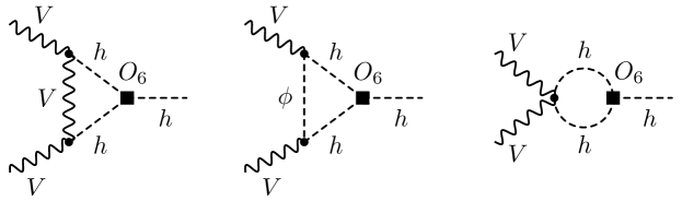
Figure 1: The three 1-loop diagrams with an insertion of the effective operator $O_{6}$ that contribute to the $VVh$ vertex at ${\cal O}(\lambda)$. Here $\phi$ denotes the relevant would-be Goldstone field that needs to be included if the calculation is performed in a $R_{\xi}$ gauge.

The integrals with a tensor structure (9) can be reduced to linear combinations of Lorentz-contravariant tensors constructed from the metric tensor $\eta^{\mu\nu}$ and a linearly independent set of the 4-momenta $p_{i}^{\mu}$. We define the tensor coefficients of the triangle integrals in the following way

$$\begin{split}C^{\mu}=\sum_{i=1,2}p_{i}^{\mu}\hskip 0.7113ptC_{i}\,,\qquad C^{\mu\nu}=\eta^{\mu\nu}\hskip 0.7113ptC_{00}+\sum_{i,j=1,2}p_{i}^{\mu}p_{j}^{\nu}\hskip 0.7113ptC_{ij}\,.\end{split}$$ (10)

Notice that of all scalar and tensor-coefficient functions appearing in our 1-loop calculations only $B_{0}$ and $C_{00}$ are ultraviolet (UV) divergent. These divergent contributions appear in our final results always in the UV-finite combination $B_{0}-4C_{00}$.

With the definitions (8), (9) and (10) at hand, the full analytic expressions of the form factors can be written as

$$\begin{split}{\cal F}_{1}(q_{1}^{2},q_{2}^{2})&=\frac{\lambda\hskip 0.7113pt\bar{c}_{6}}{(4\pi)^{2}}\left(-3B_{0}-12\left(m_{V}^{2}\hskip 0.7113ptC_{0}-C_{00}\right)-\frac{9\hskip 0.7113ptm_{h}^{2}}{2}\left(\bar{c}_{6}+2\right)B_{0}^{\prime}\right)\,,\\[5.69054pt] {\cal F}_{2}(q_{1}^{2},q_{2}^{2})&=\frac{\lambda\hskip 0.7113pt\bar{c}_{6}}{(4\pi)^{2}}\,12\,\big{(}C_{1}+C_{11}+C_{12}\big{)}\,.\end{split}$$ (11)

Here the arguments of the PV integrals are

$$B_{0}=B_{0}\big{(}m_{h}^{2},m_{h}^{2},m_{h}^{2}\big{)}\,,\qquad C_{0}=C_{0}\big{(}m_{h}^{2},q_{1}^{2},q_{2}^{2},m_{h}^{2},m_{h}^{2},m_{V}^{2}\big{)}\,,$$ (12)

and analog definitions hold for the derivative $B_{0}^{\prime}$ of the scalar bubble integral and the tensor coefficients $C_{1}$, $C_{11}$ and $C_{12}$ of the triangle integral. Notice that in contrast to Degrassi:2016wml an all-order resummation of 1-loop wave function effects is not performed in (11). Since already the ${\cal O}(\lambda^{2})$ wave function corrections in the SMEFT will be incomplete due to missing 2-loop Higgs-boson selfenergy diagrams, it is questionable if such a resummation improves the precision of the calculation and we therefore do not include it our work.

4 Corrections to the Higgs partial decay widths

To determine the signal strengths in $Vh$ and VBF Higgs production, one also has to take into account that the Higgs branching ratios are modified at the loop level by the presence of the dimension-6 operator $O_{6}$. Examples of diagrams that alter the partial widths of the Higgs to fermions, gluons and photons are displayed in Figure 2. Below we will present results for the ${\cal O}(\lambda)$ corrections to the partial widths of all relevant Higgs decay modes. Terms of ${\cal O}(\lambda^{2})$ that arise from squared matrix elements with an $O_{6}$ insertion are instead dropped for consistency since such contributions receive additional but unknown corrections from the interference of tree-level SM and loop-level SMEFT amplitudes.

In the case of the decays of the Higgs to light fermion pairs $f=q,\ell$, we write

$$\Delta\Gamma(h\to f\bar{f})=\frac{N_{c}^{f}G_{F}\hskip 0.7113ptm_{h}\hskip 0.7113ptm_{f}^{2}}{4\sqrt{2}\pi}\left(1-\frac{4\hskip 0.28453ptm_{f}^{2}}{m_{h}^{2}}\right)^{3/2}\,\Delta_{f}\,,$$ (13)

where $N_{c}^{q}=3$, $N_{c}^{\ell}=1$ and all quark masses $m_{q}$ are understood as $\overline{\rm MS}$ masses renormalised at the scale $m_{h}$, while $m_{\ell}$ denotes the pole mass of the corresponding lepton. The ${\cal O}(\lambda)$ correction to the partial decay width $\Gamma(h\to f\bar{f})$ stem from the graph displayed on the left-hand side in Figure 2. We obtain

$$\Delta_{f}=\frac{\lambda\hskip 0.7113pt\bar{c}_{6}}{(4\pi)^{2}}\,{\rm Re}\,\Big{(}-12\hskip 0.7113ptm_{f}^{2}\left(C_{0}-C_{1}-C_{2}\right)-9\hskip 0.7113ptm_{h}^{2}\left(\bar{c}_{6}+2\right)B_{0}^{\prime}\Big{)}\,,\$$ (14)

with

$$C_{0}=C_{0}\big{(}m_{f}^{2},m_{h}^{2},m_{f}^{2},m_{f}^{2},m_{h}^{2},m_{h}^{2}\big{)}\,,$$ (15)

and analogue definitions for the tensor coefficients $C_{1}$ and $C_{2}$. Notice that the flavour-dependent contributions are suppressed by light-fermion masses compared to the flavour-independent contribution proportional to $B_{0}^{\prime}$ that arises from the wave function renormalisation of the Higgs boson. The corrections $\Delta_{f}$ are hence to very good approximation universal. The result (13) agrees numerically with Degrassi:2016wml .

The shifts in the partial width for a Higgs boson decaying into a pair of EW gauge bosons can be cast into the form Grau:1990uu

$$\Delta\Gamma(h\to VV)=\frac{1}{\pi^{2}}\int_{0}^{m_{h}^{2}}\!\frac{dq_{1}^{2}\hskip 1.42262ptm_{V}\Gamma_{V}}{(q_{1}^{2}-m_{V}^{2})^{2}+m_{V}^{2}\Gamma_{V}^{2}}\int_{0}^{(m_{h}-q_{1})^{2}}\!\frac{dq_{2}^{2}\hskip 1.42262ptm_{V}\Gamma_{V}}{(q_{2}^{2}-m_{V}^{2})^{2}+m_{V}^{2}\Gamma_{V}^{2}}\;I_{V}\,,\hskip 14.22636pt$$ (16)

and include the contributions from both the production of one real and one virtual EW gauge boson $h\to VV^{\ast}$ or two virtual states $h\to V^{\ast}V^{\ast}$. In (16) the total decay width of the relevant gauge boson is denoted by $\Gamma_{V}$ and the integrand can be written as

$$I_{V}=\frac{G_{F}\hskip 0.7113ptm_{h}^{3}}{8\sqrt{2}\pi}\,N_{V}\,\sqrt{\alpha(q_{1}^{2},q_{2}^{2},m_{h}^{2})}\,\beta(q_{1}^{2},q_{2}^{2},m_{h}^{2})\,\Delta_{V}\,,$$ (17)

with $N_{W}=1$, $N_{Z}=1/2$ and

$$\alpha(x,y,z)=\left(1-\frac{x}{z}-\frac{y}{z}\right)^{2}-\frac{4\hskip 0.7113ptxy}{z^{2}}\,,\qquad\beta(x,y,z)=\alpha(x,y,z)+\frac{12\hskip 0.7113ptxy}{z^{2}}\,.$$ (18)

The ${\cal O}(\lambda)$ correction to the partial decay width $\Gamma(h\to VV)$ arises from the diagrams shown in Figure 1. We find

$$\begin{split}\Delta_{V}&=\frac{\lambda\hskip 0.7113pt\bar{c}_{6}}{(4\pi)^{2}}\,{\rm Re}\Bigg{[}-6B_{0}-24\left(m_{V}^{2}\hskip 0.7113ptC_{0}-C_{00}\right)\\[2.84526pt] &\phantom{xx}-\frac{12\hskip 0.7113pt\alpha(q_{1}^{2},q_{2}^{2},m_{h}^{2})\left(q_{1}^{2}+q_{2}^{2}-m_{h}^{2}\right)}{\beta(q_{1}^{2},q_{2}^{2},m_{h}^{2})}\,\big{(}C_{1}+C_{11}+C_{12}\big{)}-9\hskip 0.7113ptm_{h}^{2}\left(\bar{c}_{6}+2\right)B_{0}^{\prime}\Bigg{]}\,.\end{split}$$ (19)

Here the arguments of the PV loop integrals are defined as in (12). We have verified that the expression (16) agrees numerically with the results presented in Degrassi:2016wml .

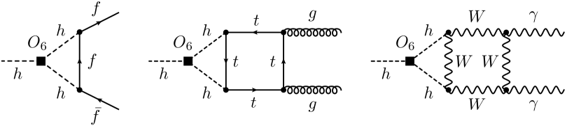
Figure 2: Feynman diagrams with an insertion of the effective operator $O_{6}$ that lead to Higgs-boson decays into fermion (left), gluon (middle) and photon (right) pairs.

The changes in partial decay widths of the Higgs boson to gluon and photon pairs can be written in the following way

$$\begin{split}\Delta\Gamma(h\to gg)&=\frac{G_{F}\hskip 0.7113pt\alpha_{s}^{2}\hskip 0.7113ptm_{h}^{3}}{36\sqrt{2}\pi^{3}}\,\bigg{|}\sum_{q}A_{q}\hskip 1.42262pt\bigg{|}^{2}\,\Delta_{g}\,,\\[5.69054pt] \Delta\Gamma(h\to\gamma\gamma)&=\frac{G_{F}\hskip 0.7113pt\alpha^{2}\hskip 0.7113ptm_{h}^{3}}{128\sqrt{2}\pi^{3}}\,\bigg{|}\sum_{f}\frac{4\hskip 0.7113ptN_{c}^{f}Q_{f}^{2}}{3}\,A_{f}-A_{W}\hskip 0.7113pt\bigg{|}^{2}\,\Delta_{\gamma}\,,\end{split}$$ (20)

where $\alpha_{s}=\alpha_{s}(m_{h})$, $\alpha=1/137.04$, while $Q_{u}=2/3$, $Q_{d}=-1/3$ and $Q_{\ell}=-1$ denote the electric charges of the fermions. The leading-order (LO) form factors that encode the 1-loop corrections due to SM fermion and $W$-boson loops read

$$\begin{split}A_{f}&=\frac{3\hskip 0.7113pt\tau_{f}}{2}\left[1+(1-\tau_{f})\arctan^{2}\frac{1}{\sqrt{\tau_{f}-1}}\right]\,,\\[8.53581pt] A_{W}&=2+3\tau_{W}+3\tau_{W}(2-\tau_{W})\arctan^{2}\frac{1}{\sqrt{\tau_{W}-1}}\,,\end{split}$$ (21)

with $\tau_{X}=4m_{X}^{2}/m_{h}^{2}$ for $X=f,W$. The ${\cal O}(\lambda)$ correction to the partial decay width of the Higgs to gluons and photons originate from 2-loop diagrams with an insertion of $O_{6}$. Two example graphs are shown in the middle and on the right of Figure 2. The results presented in Gorbahn:2016uoy ; inprep lead to

$$\begin{split}\Delta_{g}&=\frac{\lambda\hskip 0.7113pt\bar{c}_{6}}{(4\pi)^{2}}\,\big{(}8.42-9\hskip 0.7113ptm_{h}^{2}\left(\bar{c}_{6}+2\right)B_{0}^{\prime}\big{)}\,,\\[5.69054pt] \Delta_{\gamma}&=\frac{\lambda\hskip 0.7113pt\bar{c}_{6}}{(4\pi)^{2}}\,\big{(}-3.70-9\hskip 0.7113ptm_{h}^{2}\left(\bar{c}_{6}+2\right)B_{0}^{\prime}\big{)}\,.\end{split}$$ (22)

Notice that there is no need to take the real part here because the $B_{0}^{\prime}$ integral corresponding to a Higgs loop is real for on-shell kinematics. The expression for $\Delta_{g}$ agrees with the results obtained in Degrassi:2016wml .

5 Description of the $Vh$ calculation

In order to explain how we obtain our predictions for the associated production of the Higgs boson with massive gauge bosons it is useful to first consider the ${\cal O}(\lambda)$ corrections to $\sigma_{Vh}=\sigma(q\bar{q}\to Vh)$ working to zeroth order in the strong coupling constant. At this order in QCD the ${\cal O}(\lambda)$ shift in the integrated partonic cross section can be written as

$$\Delta\sigma_{Vh}=\frac{G_{F}^{2}\hskip 0.28453ptm_{V}^{4}}{72\pi\hskip 0.7113pt}\,\bar{N}_{V}\,\sqrt{\alpha(m_{V}^{2},m_{h}^{2},s)}\,\,\frac{\alpha(m_{V}^{2},m_{h}^{2},s)\,s+12\hskip 0.7113ptm_{V}^{2}}{\left(s-m_{V}^{2}\right)^{2}}\;\delta_{V}\,,$$ (23)

with $\bar{N}_{W}=1$ and $\bar{N}_{Z}=\left(1-8\hskip 0.7113ptT_{3}^{q}\hskip 0.7113ptQ_{q}s_{w}^{2}+8\hskip 0.7113ptQ_{q}^{2}s_{w}^{4}\right)/2$, where $T_{3}^{q}$ ($Q_{q})$ denotes the third component of the weak isospin (electric charge) of the relevant quark. The function $\delta_{V}$ encodes the contributions from the three 1-loop diagrams in Figure 1 when one of the gauge bosons is contracted with a quark line and the other one is put on its mass shell. Explicitly we find

$$\begin{split}\delta_{V}&=\frac{\lambda\hskip 0.7113pt\bar{c}_{6}}{(4\pi)^{2}}\,{\rm Re}\Bigg{[}-6B_{0}-24\left(m_{V}^{2}\hskip 0.7113ptC_{0}-C_{00}\right)\\[2.84526pt] &\phantom{xx}-\frac{12\hskip 0.7113pt\alpha(m_{V}^{2},m_{h}^{2},s)\,s\left(m_{V}^{2}-m_{h}^{2}+s\right)}{\alpha(m_{V}^{2},m_{h}^{2},s)\,s+12\hskip 0.7113ptm_{V}^{2}}\,\big{(}C_{1}+C_{11}+C_{12}\big{)}-9\hskip 0.7113ptm_{h}^{2}\left(\bar{c}_{6}+2\right)B_{0}^{\prime}\Bigg{]}\,,\end{split}$$ (24)

where the function $\alpha(x,y,z)$ has been defined in (18). The arguments of the scalar triangle integral are

$$C_{0}=C_{0}\big{(}m_{h}^{2},s,m_{V}^{2},m_{h}^{2},m_{h}^{2},m_{V}^{2}\big{)}\,,$$ (25)

and all other tensor coefficients carry the same functional dependence. The $B_{0}$ integral is defined in (12). Our result (24) for $\delta_{V}$ can be shown to agree with the analytic expression given in the publication McCullough:2013rea for the case of $e^{+}e^{-}\to Zh$.

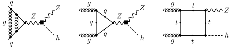
Figure 3: Examples of diagrams that contribute to $pp\to Zh$ at ${\cal O}(\alpha_{s}^{2})$. As indicated by the black square the left and middle diagram receive a correction of ${\cal O}(\lambda)$ from $\delta_{V}$, while the graph on the right-hand side does not involve a modified $ZZh$ vertex. See text for further explanations.

At NNLO the production cross section for $pp\to Vh$ receives corrections from two types of topologies. The first kind of graphs involves an exchange of a single off-shell vector boson in the $s$-channel, while the second sort of corrections arise from the coupling of the Higgs boson to a closed loop of top quarks. For on-shell bosons the former type of ${\cal O}(\alpha_{s}^{2})$ corrections have been obtained in Brein:2003wg , while fully differential NNLO calculations of these Drell-Yan (DY) parts have been presented in Ferrera:2011bk ; Ferrera:2013yga and Ferrera:2014lca for the $Wh$ and $Zh$ final state, respectively. Subsets of the diagrams where the Higgs is radiated off a top loop have been considered in Brein:2011vx ; Ferrera:2014lca and a calculation of all such graphs can be found in Campbell:2016jau . The latter results have been implemented into version 8 of MCFM Boughezal:2016wmq .

The existing fully differential MCFM implementation of $pp\to Vh$ at NNLO serves as a starting point of our own computation. We have identified the routines in MCFM that correspond to the two different kinds of ${\cal O}(\alpha_{s}^{2})$ corrections. For the case of $pp\to Zh$ representatives of the two types of contributions are displayed in Figure 3. Notice that in all diagrams where the Higgs is not radiated from a top loop the $\delta_{V}$ correction factorises and thus we are able to include the complete ${\cal O}(\lambda)$ term (24) on top of the NNLO corrections. In the case of the contributions with top loops however not all ${\cal O}(\alpha_{s}^{2})$ corrections factorise. Non-factorisable contributions which involve a top box and a top-Higgs triangle as well as double-box contributions are in fact not known and thus cannot be included. Effects due to Higgs wave function renormalisation, on the other hand, factorise and we take them into account in our computations. As a result, our numerical predictions for the differential $pp\to Vh$ cross sections are NNLO accurate only for what concerns the ${\cal O}(\lambda)$ terms associated to $\delta_{V}$, while we are missing ${\cal O}(\alpha_{s}^{2})$ contributions proportional to $\lambda\bar{c}_{6}$ that stem from top loops.

6 Description of the VBF Higgs calculation

To obtain predictions for VBF Higgs production we employ the structure-function approach Han:199hhr . In this formalism the VBF Higgs process can be described to high accuracy as a double deep-inelastic scattering process (DIS), where two virtual EW gauge bosons emitted from the hadronic initial states fuse into a Higgs boson. Neglecting small QCD-interference effects between the two inclusive final states, the differential VBF Higgs cross section is in our case given by a product of two 3-point vertices $\Gamma^{\mu\nu}_{V}(Q_{1},Q_{2})$ and two DIS hadronic tensors $W^{\mu\nu}_{V}(x_{i},Q_{i}^{2})$:

$$\begin{split}d\sigma_{\rm VBF}&=\frac{G_{F}^{2}\hskip 0.28453ptm_{V}^{4}}{s}\hskip 1.42262pt\Delta_{V}^{2}(Q_{1}^{2})\hskip 0.7113pt\Delta_{V}^{2}(Q_{2}^{2})\\[5.69054pt] &\phantom{xx}\times W_{\mu\nu}^{V}(x_{1},Q_{1}^{2})\hskip 1.42262pt\Gamma^{\mu\rho}_{V}(Q_{1},Q_{2})\hskip 0.7113pt\big{(}\Gamma^{\nu\sigma}_{V}(Q_{1},Q_{2})\big{)}^{\ast}\hskip 1.42262ptW_{\rho\sigma}^{V}(x_{2},Q_{2}^{2})\,d\Omega\,.\end{split}$$ (26)

Here $\Delta_{V}(Q_{i}^{2})=1/(Q_{i}^{2}+m_{V}^{2})$, $Q_{i}^{2}=-q_{i}^{2}$ and $x_{i}=Q^{2}_{i}/(2P_{i}\cdot q_{i})$ are the usual DIS variables with $P_{i}^{\mu}$ the 4-momentum of proton $i=1,2$ and $d\Omega$ denotes the 3-particle VBF phase space. The hadronic tensor can be expressed as

$$\begin{split}W^{\mu\nu}_{V}(x_{i},Q_{i}^{2})&=\left(-\eta^{\mu\nu}-\frac{q_{i}^{\mu}q_{i}^{\nu}}{Q_{i}^{2}}\right)F_{1}^{V}(x_{i},Q_{i}^{2})+\frac{\hat{P}_{i}^{\mu}\hat{P}_{i}^{\nu}}{P_{ii}}\,F_{2}^{V}(x_{i},Q_{i}^{2})\\[5.69054pt] &\phantom{xx}+i\epsilon^{\mu\nu\rho\sigma}\,\frac{P_{i\hskip 0.7113pt\rho}\hskip 0.7113ptq_{i\hskip 0.7113pt\sigma}}{2P_{ii}}\,F_{3}^{V}(x_{i},Q_{i}^{2})\,,\end{split}$$ (27)

where $\epsilon^{\mu\nu\rho\sigma}$ is the fully anti-symmetric Levi-Civita tensor and we have introduced

$$\qquad P_{i}\cdot q_{j}=P_{ij}\,,\qquad\hat{P}_{i}^{\mu}=P_{i}^{\mu}+\frac{P_{ii}}{Q_{i}^{2}}\,q_{i}^{\mu}\,.$$ (28)

The standard DIS structure functions are denoted by $F_{m}^{V}(x_{i},Q_{i}^{2})$ with $m=1,2,3$.

Using the decomposition (27) the squared hadronic tensor in (26) can be written in terms of the DIS structure functions as

$$\begin{split}W_{\mu\nu}^{V}(x_{1},Q_{1}^{2})\hskip 1.42262pt\Gamma^{\mu\rho}_{V}(Q_{1},Q_{2})\hskip 0.7113pt\big{(}\Gamma^{\nu\sigma}_{V}(Q_{1},Q_{2})\big{)}^{\ast}\hskip 1.42262ptW_{\rho\sigma}^{V}(x_{2},Q_{2}^{2})&=\\[5.69054pt] &4\sqrt{2}\hskip 0.7113ptG_{F}\hskip 0.7113ptm_{V}^{4}\sum_{m,n}^{3}w_{mn}\hskip 0.7113ptF_{m}^{V}(x_{1},Q_{1}^{2})\hskip 0.7113ptF_{n}^{V}(x_{2},Q_{2}^{2})\,.\end{split}$$ (29)

Defining the short-hand notations

$$q_{1}\cdot q_{2}=q_{12}\,,\quad P_{1}\cdot P_{2}=p_{12}\,,\quad{\cal C}_{1}=1+2\hskip 0.7113pt{\cal F}_{1}(Q_{1}^{2},Q_{2}^{2})\,,\quad{\cal C}_{2}=2\hskip 0.7113pt{\cal F}_{2}(Q_{1}^{2},Q_{2}^{2})\,,$$ (30)

the non-vanishing coefficients $w_{mn}$ included in our analysis read

$$\begin{split}w_{11}&=\left(2\hskip 0.7113pt{\cal C}_{1}-q_{12}\hskip 1.42262pt{\cal C}_{2}\right)+\left({\cal C}_{1}+q_{12}\hskip 1.42262pt{\cal C}_{2}\right)\hskip 0.7113pt\frac{q_{12}^{2}}{Q_{1}^{2}\hskip 0.7113ptQ_{2}^{2}}\,,\\[5.69054pt] w_{12}&=-{\cal C}_{1}\hskip 0.7113pt\frac{P_{22}}{Q_{2}^{2}}-\left({\cal C}_{1}+q_{12}\hskip 1.42262pt{\cal C}_{2}\right)\left(\frac{P_{21}^{2}}{P_{22}\hskip 0.7113ptQ_{1}^{2}}+\frac{2P_{21}\hskip 1.42262ptq_{12}}{Q_{1}^{2}\hskip 0.7113ptQ_{2}^{2}}+\frac{P_{22}\hskip 1.42262ptq_{12}^{2}}{Q_{1}^{2}\hskip 0.7113ptQ_{2}^{4}}\right)\,,\\[5.69054pt] w_{21}&=-{\cal C}_{1}\hskip 0.7113pt\frac{P_{11}}{Q_{1}^{2}}-\left({\cal C}_{1}+q_{12}\hskip 1.42262pt{\cal C}_{2}\right)\left(\frac{P_{12}^{2}}{P_{11}\hskip 0.7113ptQ_{2}^{2}}+\frac{2P_{12}\hskip 1.42262ptq_{12}}{Q_{1}^{2}\hskip 0.7113ptQ_{2}^{2}}+\frac{P_{11}\hskip 1.42262ptq_{12}^{2}}{Q_{1}^{4}\hskip 0.7113ptQ_{2}^{2}}\right)\,,\\[5.69054pt] w_{22}&=\frac{1}{P_{11}P_{22}\hskip 1.42262ptQ_{1}^{4}\hskip 0.7113ptQ_{2}^{4}}\,\Bigg{[}\,{\cal C}_{1}\,\Big{(}p_{12}\hskip 1.42262ptQ_{1}^{2}Q_{2}^{2}+P_{11}P_{21}\hskip 0.7113ptQ_{2}^{2}+P_{12}P_{22}\hskip 0.7113ptQ_{1}^{2}+P_{11}P_{22}\hskip 1.42262ptq_{12}\Big{)}^{2}\\[2.84526pt] &\phantom{xx}+{\cal C}_{2}\left(P_{12}\hskip 0.7113ptQ_{1}^{2}+P_{11}\hskip 1.42262ptq_{12}\right)\left(P_{21}\hskip 0.7113ptQ_{2}^{2}+P_{22}\hskip 1.42262ptq_{12}\right)\\[2.84526pt] &\phantom{xxxi}\times\Big{(}p_{12}\hskip 1.42262ptQ_{1}^{2}Q_{2}^{2}+P_{11}P_{21}\hskip 0.7113ptQ_{2}^{2}+P_{12}P_{22}\hskip 0.7113ptQ_{1}^{2}+P_{11}P_{22}\hskip 1.42262ptq_{12}\Big{)}\Bigg{]}\,,\\[5.69054pt] w_{33}&=\frac{1}{4P_{11}P_{22}}\,\bigg{[}\,2\hskip 0.7113pt{\cal C}_{1}\left(p_{12}\hskip 1.42262ptq_{12}-P_{12}\hskip 0.7113ptP_{21}\right)\\[2.84526pt] &\phantom{xx}-{\cal C}_{2}\,\Big{\{}P_{12}P_{22}\hskip 0.7113ptQ_{1}^{2}+\left(p_{12}\hskip 1.42262ptQ_{1}^{2}+P_{11}P_{21}\right)Q_{2}^{2}+\left(P_{11}P_{22}+P_{12}P_{21}\right)q_{12}-p_{12}\hskip 1.42262ptq_{12}^{2}\Big{\}}\,\bigg{]}\,.\end{split}$$ (31)

Notice that in the above expressions for the coefficients $w_{mn}$ we have neglected terms quadratic in the form factors ${\cal F}_{1,2}(Q_{1}^{2},Q_{2}^{2})$. Such contributions are suppressed relative to the linear terms in (31) by a factor of $\lambda\bar{c}_{6}/(4\pi)^{2}$ and thus formally of 2-loop order in the SMEFT. Since the 2-loop SMEFT contributions to the ${\cal O}(\lambda^{2})$ corrections remain unknown including terms quadratic in (11) would thus not improve the accuracy of the calculation.

With all the non-vanishing coefficients $w_{mn}$ at hand it is now rather straightforward to calculate NNLO QCD corrections to the inclusive Bolzoni:2010xr ; Bolzoni:2011cu and exclusive Cacciari:2015jma VBF Higgs cross section. Our computations rely on the techniques and the Monte Carlo (MC) codes developed in the latter work. In the inclusive part of the calculation, we employ the phase space from the $h+2\,{\rm jets}$ VBF calculation implemented in POWHEG Nason:2009ai , while the matrix element is evaluated with structure functions based on parametrised versions vanNeerven:1999ca ; vanNeerven:2000uj of the NNLO DIS coefficient functions vanNeerven:1991nn ; Zijlstra:1992qd ; Zijlstra:1992kj integrated with HOPPET Salam:2008qg . The exclusive calculation relies also on the NLO part of the POWHEG $h+3\,{\rm jets}$ VBF code Jager:2014vna , which implements the results of Figy:2007kv . To take into account contributions from the second Lorentz structure in (7) the SM implementation Jager:2014vna had to be extended. This extension required, in particular, new tree-level $h+4\,{\rm jets}$ matrix elements, which were generated with MadGraph5_aMCNLO Alwall:2014hca . The numerical evaluation of 1-loop Feynman integrals is performed by QCDLoop Ellis:2007qk ; Carrazza:2016gav after reducing the tensor coefficients appearing in (9) to basic PV scalar integrals. Further technical details on the implementation of the NNLO VBF Higgs cross section computations are given in Cacciari:2015jma .

7 Numerical results

In this section we study the numerical impact of the ${\cal O}(\lambda)$ corrections that we have derived earlier in Sections 3 and 4. We first present results for the modifications of the Higgs production cross sections $\sigma_{I}$ in the vector boson mediated channels $I=Wh,Zh,{\rm VBF}$. Then we study the corrections to the partial Higgs decay widths $\Gamma^{F}=\Gamma(h\to F)$ and branching ratios ${\rm Br}^{F}={\rm Br}(h\to F)$. This discussion is followed by an analysis of the shape changes in the $Vh$ and VBF Higgs distributions due to the ${\cal O}(\lambda)$ corrections. We finally derive the constraints on the Wilson coefficient $\bar{c}_{6}$ that arise from LHC Run I and II data, and explore the prospects of the HL-LHC in improving the current bounds. Both the limits from double-Higgs production as well as $Vh$ and VBF Higgs production are considered.

7.1 Modifications of the Higgs production cross sections

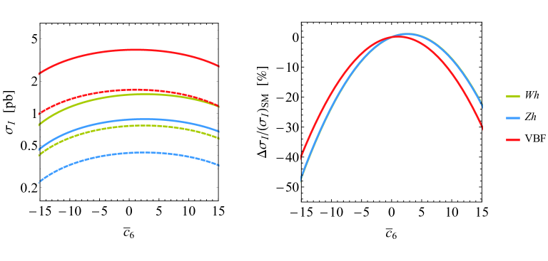
Figure 4: Left: Predictions for the inclusive $Wh$, $Zh$ and VBF Higgs production sections $\sigma_{I}$ as a function of $\bar{c}_{6}$. The dashed and solid curves correspond to $\sqrt{s}=8\,{\rm TeV}$ and $\sqrt{s}=13\,{\rm TeV}$, respectively. Right: Relative modifications of $\sigma_{I}$ as a function of the Wilson coefficient of $O_{6}$. Only results for $\sqrt{s}=13\,{\rm TeV}$ are shown.

We begin our discussion by considering the modifications of the inclusive vector boson mediated Higgs production sections $\sigma_{I}$ that result from the presence of the ${\cal O}(\lambda)$ corrections. The corresponding predictions are shown in the two panels of Figure 4 as a function of $\bar{c}_{6}$. In the left plot we display the total cross sections for $pp$ collisions at $\sqrt{s}=8\,{\rm TeV}$ (dashed curves) and $\sqrt{s}=13\,{\rm TeV}$ (solid curves). In the former case, we find

$$\begin{split}\sigma_{Wh}^{8\,{\rm TeV}}&=(\sigma_{Wh}^{8\,{\rm TeV}})_{\rm SM}\left(1+7.4\cdot 10^{-3}\hskip 2.84526pt\bar{c}_{6}-1.5\cdot 10^{-3}\hskip 2.84526pt\bar{c}_{6}^{2}\right)\,,\\[5.69054pt] \sigma_{Zh}^{8\,{\rm TeV}}&=(\sigma_{Zh}^{8\,{\rm TeV}})_{\rm SM}\left(1+7.5\cdot 10^{-3}\hskip 2.84526pt\bar{c}_{6}-1.5\cdot 10^{-3}\hskip 2.84526pt\bar{c}_{6}^{2}\right)\,,\\[5.69054pt] \sigma_{\rm VBF}^{8\,{\rm TeV}}&=(\sigma_{\rm VBF}^{8\,{\rm TeV}})_{\rm SM}\left(1+3.3\cdot 10^{-3}\hskip 2.84526pt\bar{c}_{6}-1.5\cdot 10^{-3}\hskip 2.84526pt\bar{c}_{6}^{2}\right)\,,\end{split}$$ (32)

where the prediction for the $Wh$ cross section includes both the $pp\to W^{+}h$ and the $pp\to W^{-}h$ channel. The SM predictions that enter the above formulas read $(\sigma_{Wh}^{8\,{\rm TeV}})_{\rm SM}=(0.76\pm 0.02)\,{\rm pb}$, $(\sigma_{Zh}^{8\,{\rm TeV}})_{\rm SM}=(0.42\pm 0.01)\,{\rm pb}$ and $(\sigma_{\rm VBF}^{8\,{\rm TeV}})_{\rm SM}=(1.66\pm 0.04)\,{\rm pb}$. In the latter case, we instead obtain

$$\begin{split}\sigma_{Wh}^{13\,{\rm TeV}}&=(\sigma_{Wh}^{13\,{\rm TeV}})_{\rm SM}\left(1+8.2\cdot 10^{-3}\hskip 2.84526pt\bar{c}_{6}-1.5\cdot 10^{-3}\hskip 2.84526pt\bar{c}_{6}^{2}\right)\,,\\[5.69054pt] \sigma_{Zh}^{13\,{\rm TeV}}&=(\sigma_{Zh}^{13\,{\rm TeV}})_{\rm SM}\left(1+8.0\cdot 10^{-3}\hskip 2.84526pt\bar{c}_{6}-1.5\cdot 10^{-3}\hskip 2.84526pt\bar{c}_{6}^{2}\right)\,,\\[5.69054pt] \sigma_{\rm VBF}^{13\,{\rm TeV}}&=(\sigma_{\rm VBF}^{13\,{\rm TeV}})_{\rm SM}\left(1+3.3\cdot 10^{-3}\hskip 2.84526pt\bar{c}_{6}-1.5\cdot 10^{-3}\hskip 2.84526pt\bar{c}_{6}^{2}\right)\,,\end{split}$$ (33)

and the relevant SM cross sections are $(\sigma_{Wh}^{13\,{\rm TeV}})_{\rm SM}=(1.49\pm 0.03)\,{\rm pb}$, $(\sigma_{Zh}^{13\,{\rm TeV}})_{\rm SM}=(0.87\pm 0.03)\,{\rm pb}$ and $(\sigma_{\rm VBF}^{13\,{\rm TeV}})_{\rm SM}=(3.94\pm 0.08)\,{\rm pb}$. Our results have been obtained with the implementations of the $Vh$ and VBF Higgs calculations described in Sections 5 and 6. They correspond to PDF4LHC15_nnlo_mc parton distribution functions (PDFs) Butterworth:2015oua and the quoted uncertainties include both scale, PDF and $\alpha_{s}$ errors. In the case of $Vh$ (VBF Higgs) production our default scale choice is $\mu_{0}=m_{V}+m_{h}$ ($\mu_{0}=m_{h}$). The perturbative uncertainties are estimated in both cases by identifying the renormalisation and factorisation scales $\mu_{R}$ and $\mu_{F}$ with $\mu_{0}$ and varying $\mu_{0}$ by a factor of two around the default scale.

The above formulas can be compared to the next-to-leading order (NLO) results for the $Vh$ and VBF Higgs production cross sections presented in Degrassi:2016wml . Concerning $\sigma_{Wh}$ and $\sigma_{\rm VBF}$, we find that the inclusion of ${\cal O}(\alpha_{s}^{2})$ corrections essentially does not change the functional dependence on $\bar{c}_{6}$ compared to NLO. In the case of $\sigma_{Zh}$, NNLO effects have instead an impact since they shift the term linear in $\bar{c}_{6}$ by around $-20\%$ ($-10\%$) compared to the $8\,{\rm TeV}$ ($13\,{\rm TeV}$) NLO prediction. The observed shifts originate from the negative ${\cal O}(\alpha_{s}^{2})$ contributions due to heavy-quark boxes of the type $gg\to Zh$. Given that the corresponding non-universal ${\cal O}(\lambda)$ corrections are not included in our calculation (see the discussion in Section 5) it remains unclear whether the inclusion of NNLO effects improves the precision of our $pp\to Zh$ predictions. We add that we have verified that at NLO our numerical results for $Vh$ and VBF Higgs production all agree with the predictions given in Degrassi:2016wml .

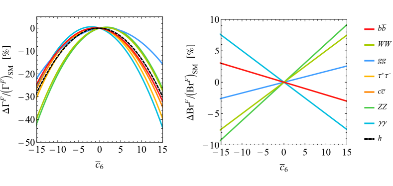
Figure 5: Shifts in the partial decay widths (left panel) and the branching ratios (right panel) of the Higgs boson as a function of the Wilson coefficient $\bar{c}_{6}$. The coloured curves indicate the individual decay channels, while the black dashed curve corresponds to the total Higgs decay width.

Looking at the results (32) and (33) one observes that the linear dependence on the Wilson coefficient $\bar{c}_{6}$ of the $Vh$ and VBF Higgs cross sections is different. This feature is expected because the terms linear in $\bar{c}_{6}$ originate from both tree-level counterterm graphs involving a Higgs wave function renormalisation as well as the interference of tree-level with 1-loop amplitudes. While the Higgs wave function renormalisation constant depends only on $m_{h}$, the interference contributions have a non-trivial dependence on the external 4-momenta. As a result the ${\cal O}(\bar{c}_{6})$ terms are process and kinematics dependent. To better illustrate the numerical impact of the ${\cal O}(\lambda)$ corrections, we plot $\Delta\sigma_{I}/(\Delta\sigma_{I})_{\rm SM}$ as a function of $\bar{c}_{6}$ in the right panel of Figure 4 employing $\sqrt{s}=13\,{\rm TeV}$. We see that for $\bar{c}_{6}\simeq-15$ the $Vh$ and VBF Higgs cross sections are shifted by about $-50\%$ and $-40\%$, while for $\bar{c}_{6}\simeq 15$ the corresponding shifts are around $-25\%$ and $-30\%$. Given that the functional dependencies of (32) and (33) are approximately the same, effects of similar size are obtained at $\sqrt{s}=8\,{\rm TeV}$. The corresponding predictions are not shown in the latter figure.

7.2 Modifications of the Higgs decays

We now turn our attention to the partial decay widths and branching ratios of the Higgs. In Figure 5 we illustrate the numerical impact of the ${\cal O}(\lambda)$ corrections on these observables. As input parameters we have used $\alpha_{s}(m_{h})=0.1127$, $m_{t}=173.2\,{\rm GeV}$, $m_{b}(m_{h})=2.81\,{\rm GeV}$, $m_{c}(m_{h})=0.65\,{\rm GeV}$, $m_{\tau}=1.777\,{\rm GeV}$, $m_{W}=80.37\,{\rm GeV}$, $m_{Z}=91.15\,{\rm GeV}$, $\Gamma_{W}=2.0886\,{\rm GeV}$ and $\Gamma_{Z}=2.4958\,{\rm GeV}$. The quoted values for the bottom and charm quark $\overline{\rm MS}$ masses have been obtained by employing 2-loop running. The SM predictions for the total decay width of the Higgs and its branching ratios are taken from YR4 . In the case of the partial decay widths (left panel), one observes that the relative corrections to $\Gamma^{F}$ all have a very similar $\bar{c}_{6}$ dependence and are essentially always negative. These features are related to the fact that for $|\bar{c}_{6}|\gtrsim 1$ the partial decay widths are dominated by the universal corrections arising from the Higgs wave function renormalisation which is quadratic in $\bar{c}_{6}$ and carries a minus sign. Numerically, we find that the relative shifts in $\Gamma^{F}$ can reach up to around $-40\%$ ($-45\%$) for $\bar{c}_{6}\simeq-15$ ($\bar{c}_{6}\simeq 15$). The corrections to the total decay width $\Gamma_{h}$ are only about $-30\%$. In the case of the shifts in the Higgs branching ratios (right panel), one observes instead that the modifications in all channels do not exceed $\pm 10\%$ in the same $\bar{c}_{6}$ range. The impact of ${\cal O}(\lambda)$ corrections is thus generically smaller in the branching ratios than in the partial decay widths, since in the former quantities the universal Higgs wave function corrections and thus the quadratic dependence on $\bar{c}_{6}$ cancels.

7.3 Modifications of the $Vh$ and VBF Higgs distributions

Since the vertex corrections (7) depend in a non-trivial way on the external 4-momenta, the ${\cal O}(\lambda)$ corrections not only change the overall size of the cross sections in $Vh$ and VBF Higgs production but also modify the shape of the corresponding kinematic distributions. In this subsection we present results for the spectra that are most sensitive to modifications in the trilinear Higgs coupling. All results shown below correspond to $\sqrt{s}=13\,{\rm TeV}$, PDF4LHC15_nnlo_mc PDFs and the default scale choices introduced in Section 7.1. Off-shell effects in Higgs-boson production are taken into account by modelling the width of the Higgs with a Breit-Wigner line shape.

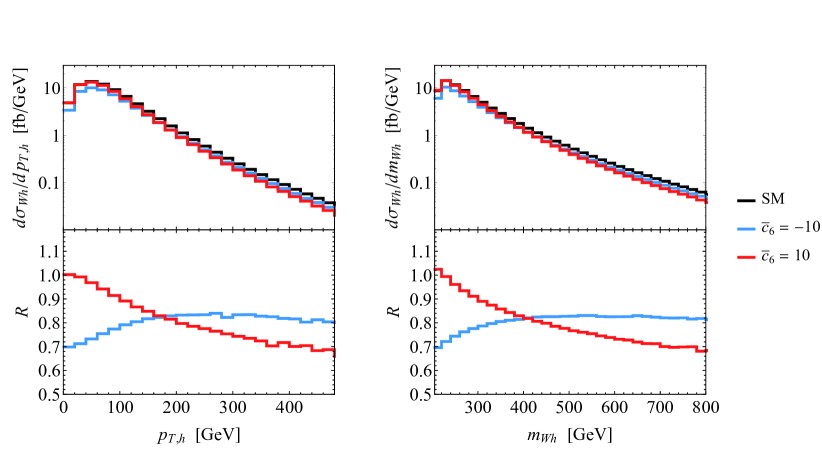
Figure 6: Comparison of the $p_{T,h}$ (left) and $m_{Wh}$ (right) spectrum in $Wh$ production. The upper panels show the SM predictions (black) as well as the cases $\bar{c}_{6}=-10$ (blue) and $\bar{c}_{6}=10$ (red). The ratios between the case $\bar{c}_{6}=-10$ and the SM (blue) and the case $\bar{c}_{6}=10$ and the SM (red) are displayed in the lower panels. All results correspond to $pp$ collisions at $\sqrt{s}=13\,{\rm TeV}$.

We begin our discussion with $pp\to Wh$. In Figure 6 the distributions of the Higgs-boson transverse momentum ($p_{T,h}$) and the invariant mass of the $Wh$ system ($m_{Wh}$) are shown. The black curves in the panels represent the SM predictions, while the blue and red curves correspond to a new-physics scenario with $\bar{c}_{6}=-10$ and $\bar{c}_{6}=10$, respectively. All results have been obtained at NNLO with the MC code described in Section 5. One sees that the shape of the displayed distributions provide sensitivity to the sign of $\bar{c}_{6}$. In the case of $\bar{c}_{6}=-10$ the $p_{T,h}$ ($m_{Wh}$) spectrum increases relative to the SM distribution as a function of $p_{T,h}$ ($m_{Wh}$), approaching a constant value in the limit of large $p_{T,h}$ ($m_{Wh}$). For $\bar{c}_{6}=10$ the ratio $R$ instead decreases with $p_{T,h}$ ($m_{Wh}$) becoming again flat for $p_{T,h}\to\infty$ ($m_{Wh}\to\infty$). The behaviour of the distribution for large $p_{T,h}$ and $m_{Wh}$ can be understood from the $\sqrt{s}\to\infty$ limit of (24). In this limit only the Higgs wave function renormalisation contributes and the vertex correction $\delta_{V}$ takes the simple form

$$\lim_{\sqrt{s}\to\infty}\delta_{V}=\frac{\lambda\hskip 0.7113pt\bar{c}_{6}}{(4\pi)^{2}}\left(-9\hskip 0.7113ptm_{h}^{2}\left(\bar{c}_{6}+2\right)B_{0}^{\prime}\right)=-1.5\cdot 10^{-3}\;\bar{c}_{6}\left(\bar{c}_{6}+2\right)\,.$$ (34)

It follows that for large transverse momenta (invariant masses) the deviation from 1 of the ratio $R$ of the $p_{T,h}$ ($m_{Wh}$) spectrum for $\bar{c}_{6}\neq 0$ and $\bar{c}_{6}=0$, i.e. the SM distribution, is approximately given by (34). New-physics scenarios with $\bar{c}_{6}<0$ will hence lead to harder $p_{T,h}$ and $m_{Wh}$ tails than cases with $\bar{c}_{6}>0$, while they predict softer spectra at low $p_{T,h}$ and $m_{Wh}$. These features are clearly visible in Figure 6 and are also present in other kinematical observables such as the transverse momentum $p_{T,W}$ of the $W$ boson. The shapes of all rapidity distributions in $pp\to Wh$ production are in contrast largely insensitive to the sign of $\bar{c}_{6}$. Notice that our general arguments also apply to the case of $pp\to Zh$, and as a result the distributions in the $Zh$ channel resemble those found in $Wh$ production. We therefore do not show predictions for the various $Zh$ spectra.

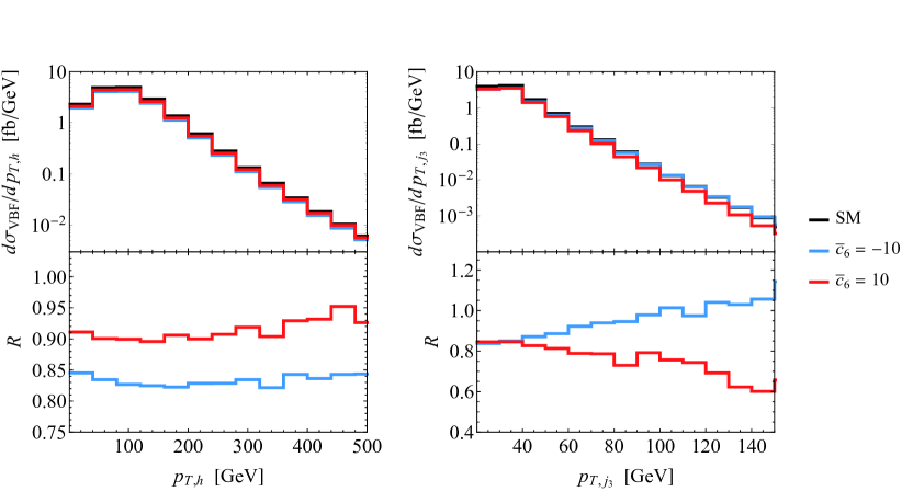
Figure 7: Comparison of the $p_{T,h}$ (left) and $p_{T,j_{3}}$ (right) spectrum in VBF Higgs production. The style and colour coding of the curves follows the one of Figure 6.

In Figure 7 we present our results for two kinematic distributions in VBF Higgs production, namely the Higgs transverse momentum $p_{T,h}$ and the transverse momentum of the third jet $p_{T,j_{3}}$. The spectra shown are obtained with the fully-differential NNLO VBF code described in Section 6 and correspond to the following selection cuts. Events should have at least two jets with $p_{T,j}>25\,{\rm GeV}$, the two jets with highest $p_{T,j}$ are required to have an absolute rapidity of $|y_{j}|<4.5$, be separated by $\Delta y_{j_{1},j_{2}}>5$ in rapidity, have an invariant mass $m_{j_{1},j_{2}}>600\,{\rm GeV}$ and be in opposite hemispheres (i.e. $y_{j_{1}}y_{j_{2}}<0$). In our analysis jets are defined using the anti-$k_{t}$ algorithm Cacciari:2008gp , as implemented in FastJet Cacciari:2011ma , with radius parameter of $0.4$. As before we present results for the benchmark scenarios $\bar{c}_{6}=-10$ (blue curves) and $\bar{c}_{6}=10$ (red curves) and compare them to the SM predictions (black curves). From the left panel in the figure we see that the shape of the $p_{T,h}$ distribution in VBF Higgs production is modified only mildly by the presence of new physics in the $h^{3}$ coupling, and in consequence the ratio to the SM is almost constant in $p_{T,h}$. This feature can be explained by realising that even for large $p_{T,h}$ one of the squared momenta $Q_{1}^{2}$ or $Q_{2}^{2}$ that enters the form factors ${\cal F}_{1,2}(Q_{1}^{2},Q_{2}^{2})$ $\big{(}$see (30)$\big{)}$ can be small. As a result for fixed $p_{T,h}$ a range of $Q_{1,2}^{2}$ values is probed and the constant ratio to the SM reflects this averaging. Similar averagings also take place for instance for the transverse momentum of the first and second hardest jet, and hence the ratios $R$ corresponding to $p_{T,j_{1}}$ and $p_{T,j_{2}}$ turn out to be almost flat as well. On the contrary, when the third jet is hard both $Q_{1,2}^{2}$ tend to be hard. An increase in magnitude of both $Q_{1,2}^{2}$ gives rise to an approximately linear modification of the form factors ${\cal F}_{1,2}(Q_{1}^{2},Q_{2}^{2})$. This results in a linear shape in the ratio to the SM, as can be seen from the right panel in Figure 7. Still the effects are relatively small for the $p_{T,j_{3}}$ values accessible at the LHC, which will limit the discriminating power of shape analyses in the VBF Higgs production channel.

7.4 Constraints on $\bar{c}_{6}$ from double-Higgs production

In the next subsection will derive the existing and possible future limits on the modifications of the trilinear Higgs-boson coupling that arise from $Vh$ and VBF Higgs production. All the numbers that we will present should be compared to the bounds that one can obtain by studying $pp\to hh$ production at the LHC. For definiteness we will assume throughout our numerical analysis that the modifications of the Wilson coefficient of the operator $O_{6}$ furnish the dominant contribution to the observable under consideration, and consequently neglect effects associated to other dimension-6 operators such as for instance $O_{H}$ — see (4).

The ATLAS collaboration has recently performed a search for Higgs-boson pair production in the $2b2\bar{b}$ final state using $13.3\,{\rm fb}^{-1}$ of $\sqrt{s}=13\,{\rm TeV}$ data ATLAS-CONF-2016-049 . From this measurement the cross section times branching ratio for non-resonant SM Higgs-boson pair production is constrained to be less than $330\,{\rm fb}$, which is approximately 29 times above the SM expectation of $(\sigma_{2b2\bar{b}}^{13\,{\rm TeV}})_{\rm SM}=(11.3^{+0.9}_{-1.0})\,{\rm pb}$. By employing HPAIR Grober:2015cwa ; hpair , we obtain

$$\sigma_{2b2\bar{b}}^{13\,{\rm TeV}}=(\sigma_{2b2\bar{b}}^{13\,{\rm TeV}})_{\rm SM}\ \left(1-0.82\hskip 0.7113pt\bar{c}_{6}+0.29\hskip 0.7113pt\bar{c}_{6}^{2}\right){\rm pb}\,.$$ (35)

From this formula we find that the ATLAS limit on the $pp\to 2h\to 2b2\bar{b}$ production cross section translates into the following 95% confidence level (CL) bound

$$\bar{c}_{6}\in[-9.5,12.3]\,,$$ (36)

if theoretical uncertainties are taken into account. Note that (36) improves on the bound of $\bar{c}_{6}\in[-15.5,18.1]$ that has been derived in Gorbahn:2016uoy from the ATLAS Run I searches for $pp\to hh$ Aad:2014yja ; Aad:2015uka ; Aad:2015xja by around $35\%$. It follows that the combination $\lambda c_{3}$ introduced in (5) can at present still deviate from the SM trilinear Higgs coupling $\lambda$ by a factor of roughly 11.

The small rate, the mild dependence of the cross section on $\lambda$ and the difficulty of selecting signal from backgrounds make determinations of the trilinear Higgs coupling in $pp\to 2h$ production challenging even at the HL-LHC. For instance the ATLAS study of the $2b2\gamma$ final state ATL-PHYS-PUB-2014-019 foresees a 95% CL limit of

$$\bar{c}_{6}\in[-2.3,7.7]\,,$$ (37)

assuming $3\,{\rm ab}^{-1}$ of integrated luminosity. Multivariate analyses (MVAs) and/or combinations of $2b2\gamma$ with other decay channels such as $2\tau 2b$ ATL-PHYS-PUB-2015-046 or $2b2\bar{b}$ may allow to improve (37), by how much precisely is however unclear at present.

7.5 Constraints on $\bar{c}_{6}$ from $Vh$ and VBF Higgs production

Since only the product of the production cross sections $\sigma_{I}$ and branching ratios ${\rm Br}^{F}$ of the Higgs boson can be extracted experimentally, it has become customary to define the signal strengths

$$\mu_{I}^{F}=\frac{\sigma_{I}}{(\sigma_{I})_{\rm SM}}\,\frac{{\rm Br}^{F}}{({\rm Br}^{F})_{\rm SM}}\,,$$ (38)

which characterise the Higgs boson yields in a specific production and decay channel relative to the SM expectations. The formalisms of signal strengths can then be used to test the compatibility of the LHC measurements with the SM and to interpret the Higgs data in the context of BSM searches.

To obtain the current constraints on $\bar{c}_{6}$ we use the LHC Run I combination of the ATLAS and CMS measurements of the Higgs boson production and decay rates ATLASCMS . In the case of the vector boson mediated production processes the relevant $\mu_{I}^{F}$ parameters read

$$\begin{split}&\hskip 49.79231pt\mu_{V}^{b\bar{b}}=0.65^{+0.30}_{-0.29}\,,\qquad\mu_{V}^{WW}=1.38^{+0.41}_{-0.37}\,,\\[5.69054pt] &\mu_{V}^{\tau^{+}\tau^{-}}=1.12^{+0.37}_{-0.35}\,,\qquad\mu_{V}^{ZZ}=0.48^{+1.37}_{-0.91}\,,\qquad\mu_{V}^{\gamma\gamma}=1.05^{+0.44}_{-0.41}\,,\end{split}$$ (39)

where the subscript $V$ indicates that the above numbers correspond to a combination of the $Vh$ and ${\rm VBF}$ channels. These numbers have been obtained from a 10-parameter fit to each of the five decay channels and can be found in the upper part of Table 13 of ATLASCMS . The quoted uncertainties take into account the experimental uncertainty in the measurement of $\mu_{I}^{F}$ as well as the SM theory error associated to each particular channel. In the following we will employ this framework to set limits on the Wilson coefficient $\bar{c}_{6}$.

Using our predictions for $\sigma_{I}$ and ${\rm Br}^{F}$ presented in Sections 7.1 and 7.2 we then can calculate the signal strengths $\mu_{I}^{F}$ and compare them to experiment. Including the errors quoted in (39) but neglecting theoretical uncertainties associated to missing $\lambda$ terms, we obtain the limit

$$\bar{c}_{6}\in[-13.6,16.9]\,,\quad{\text{(LHC Run I)}}\,,$$ (40)

by performing a $\chi^{2}$ fit with $\Delta\chi^{2}=3.84$ which corresponds to a 95% CL for a Gaussian distribution. This constraint is somewhat weaker than both the bound (36) as well as the limit of $\bar{c}_{6}\in[-11.9,10.3]$ that follows from a combination of the $gg\to h$ and $h\to\gamma\gamma$ channels Gorbahn:2016uoy ; inprep . Notice that our bound (40) compares well with the current limits on the modifications of the trilinear Higgs coupling reported in Degrassi:2016wml .

The experimental prospects for measuring the Higgs boson signal strengths (38) in the vector boson mediated production modes at future LHC runs has been studied by both the ATLAS and CMS collaborations ATL-PHYS-PUB-2014-011 ; ATL-PHYS-PUB-2014-012 ; ATL-PHYS-PUB-2014-016 ; ATL-PHYS-PUB-2014-018 ; ATL-PHYS-PUB-2016-008 ; CMS:2013xfa . To estimate the sensitivity on $\bar{c}_{6}$ that can be reached at the HL-LHC with $3\,{\rm ab}^{-1}$ of data, we study two benchmark scenarios based on the results reported in the fourth and fifth column of Table 1 of ATL-PHYS-PUB-2014-016 . Our first scenario includes the current theory uncertainties and reads

$$\begin{split}&\hskip 99.58464pt\Delta\mu_{Wh}^{b\bar{b}}=\pm 37\%\,,\quad\Delta\mu_{Wh}^{\gamma\gamma}=\pm 19\%\,,\\[5.69054pt] &\hskip 59.75095pt\Delta\mu_{Zh}^{b\bar{b}}=\pm 14\%\,,\quad\Delta\mu_{Zh}^{\gamma\gamma}=\pm 28\%\,,\quad\Delta\mu_{Vh}^{ZZ}=\pm 13\%\,,\\[5.69054pt] &\Delta\mu_{\rm VBF}^{WW}=\pm 15\%\,,\quad\Delta\mu_{\rm VBF}^{\tau^{+}\tau^{-}}=\pm 19\%\,,\quad\Delta\mu_{\rm VBF}^{ZZ}=\pm 21\%\,,\quad\Delta\mu_{\rm VBF}^{\gamma\gamma}=\pm 22\%\,,\end{split}$$ (41)

whereas in the second benchmark scenario theoretical errors are not taken into account. The corresponding relative uncertainties are

$$\begin{split}&\hskip 99.58464pt\Delta\mu_{Wh}^{b\bar{b}}=\pm 36\%\,,\quad\Delta\mu_{Wh}^{\gamma\gamma}=\pm 17\%\,,\\[5.69054pt] &\hskip 59.75095pt\Delta\mu_{Zh}^{b\bar{b}}=\pm 13\%\,,\quad\Delta\mu_{Zh}^{\gamma\gamma}=\pm 27\%\,,\quad\Delta\mu_{Vh}^{ZZ}=\pm 12\%\,,\\[5.69054pt] &\Delta\mu_{\rm VBF}^{WW}=\pm 9\%\,,\quad\Delta\mu_{\rm VBF}^{\tau^{+}\tau^{-}}=\pm 15\%\,,\quad\Delta\mu_{\rm VBF}^{ZZ}=\pm 16\%\,,\quad\Delta\mu_{\rm VBF}^{\gamma\gamma}=\pm 15\%\,.\end{split}$$ (42)

Notice that compared to the CMS projections ATL-PHYS-PUB-2016-008 our HL-LHC benchmark uncertainties $\Delta\mu_{I}^{F}$ are comparable but in all cases slightly larger, irrespectively of whether or not theory errors are included in the final numbers.

Assuming that the central values of the future HL-LHC measurements coincide in every channel with the predictions of the SM, we obtain the following 95% CL limit on the Wilson coefficient of $O_{6}$ from our $\chi^{2}$ fit

$$\bar{c}_{6}\in[-7.0,10.9]\,,\quad{\text{(HL-LHC, all uncertainties)}}\,,$$ (43)

when all uncertainties are included. If theoretical errors are neglected, we instead find

$$\bar{c}_{6}\in[-6.2,9.6]\,,\quad{\text{(HL-LHC, no theory uncertainty)}}\,.$$ (44)

These limits improve on the current constraint (40) by a factor of around 1.7 to 2, depending on how theory errors are treated. They should be compared to the determination (37) of $\bar{c}_{6}$ in double-Higgs production. We see that with the full HL-LHC data set the indirect determination of $\bar{c}_{6}$ through measurements of $pp\to Vh$ and $pp\to jjh$ should allow to test shifts in the trilinear Higgs coupling that are at the same level than the more direct extraction via $pp\to hh$. A comparison of (43) and (44) also shows that theoretical uncertainties are not a limiting factor for the extraction of $\bar{c}_{6}$ through measurements of $Vh$ and VBF Higgs production.

We finally add that future LHC combinations of the cross section measurements of $pp\to Vh$ and $pp\to jjh$ with those of $gg\to h$ Gorbahn:2016uoy ; Degrassi:2016wml and $pp\to t\bar{t}h$ Degrassi:2016wml are expected to further strengthen the indirect constraints on the Wilson coefficient of the operator $O_{6}$. Differential information from single Higgs production and/or decays may also be used to improve the sensitivity on $\bar{c}_{6}$. Making the latter statement more precise would require a MVA of the prospects to measure $Vh$ and VBF Higgs distributions in the HL-LHC environment building on the results presented in Section 7.3. Such a study is however beyond the scope of this article.

8 Conclusions

The main goal of this work was to constrain possible deviations in the $h^{3}$ coupling using measurements of $Vh$ and VBF Higgs production in $pp$ collisions. In order to keep the entire discussion model independent, we have adopted the SMEFT framework, in which the effects of new heavy particles are encoded in the Wilson coefficients of higher-dimensional operators. Within the SMEFT, we have calculated the ${\cal O}(\lambda)$ corrections to the $pp\to Vh$ and $pp\to jjh$ amplitudes that arise from insertions of the operator $O_{6}=-\lambda\left(H^{\dagger}H\right)^{3}$ into 1-loop Feynman diagrams. We have supplemented this calculation by a computation of the ${\cal O}(\lambda)$ corrections to the partial decay widths of the Higgs boson in $h\to f\bar{f}$, $h\to VV$, $h\to gg$ and $h\to\gamma\gamma$. By combining both calculations we are able to derive the full ${\cal O}(\lambda)$ corrections to all phenomenological relevant vector boson mediated Higgs signal strengths.

To obtain accurate predictions for the $pp\to Vh$ and $pp\to jjh$ our MC simulations include QCD corrections up to NNLO. We have studied the impact of a modified $h^{3}$ vertex on the inclusive cross sections and the most important kinematic distributions in $Vh$ and VBF Higgs production. The dependencies of the inclusive production cross sections on $\bar{c}_{6}$ turn out to be process dependent and slightly stronger in the $Vh$ channels than in VBF Higgs production. Since the ${\cal O}(\lambda)$ corrections to the $VVh$ vertex depend in a non-trivial way on the external 4-momenta, the $\bar{c}_{6}$ dependence is also sensitive to the kinematic configurations of the final state under consideration. Our study of kinematic distributions in $pp\to Vh$ and $pp\to jjh$ shows that the shapes of the transverse momentum or invariant mass spectra in these channels are sensitive to both the size and sign of $\bar{c}_{6}$. However a more detailed analysis than the one performed in our article is required to determine to which extent differential information in $Vh$ and VBF Higgs production can be used to improve the constraints on $\bar{c}_{6}$ that can be derived using inclusive rates. We plan to return to this question in future work.

Under the assumption that $\bar{c}_{6}$ is the only Wilson coefficient that obtains a non-zero correction in the SMEFT, we have then studied the sensitivity of present and future LHC measurements of $Vh$ and VBF Higgs production to a modified $h^{3}$ interaction. We have first demonstrated that the constraint on $\bar{c}_{6}$ that follows from a combination of the LHC Run I measurements of signal strengths in $Vh$ and VBF Higgs production are slightly more stringent than the limit obtained from double-Higgs production using Run I data. In the case of the HL-LHC with $3\,{\rm ab}^{-1}$ of integrated luminosity, we have furthermore found that it should be possible to improve the present bound by a factor of at least 1.7. As a result indirect determinations of $|\bar{c}_{6}|\lesssim 9$ based on $Vh$ and VBF Higgs production data alone should be possible. This conservative limit is not significantly weaker than the bound obtained by the ATLAS sensitivity study ATL-PHYS-PUB-2014-019 from double-Higgs production at the HL-LHC.

Further improvements of the constraints on the trilinear Higgs coupling are possible by combining the signal strength measurements in $pp\to Vh$ and $pp\to jjh$ with those in $gg\to h$ Gorbahn:2016uoy ; Degrassi:2016wml and $pp\to t\bar{t}h$ Degrassi:2016wml . The indirect probes of the trilinear Higgs coupling studied here and in Gorbahn:2016uoy ; Degrassi:2016wml hence provide information that is complementary to the direct determinations of $\lambda$ through $pp\to hh$ production. Since the indirect and direct tests constrain different linear combinations of effective operators in the SMEFT, we believe that it is crucial to combine all available information on the $h^{3}$ coupling in the form of a global fit to fully exploit the potential of the HL-LHC. We look forward to further theoretical but also experimental investigations in this direction.

- (1) The ATLAS and CMS Collaborations, ATLAS-CONF-2015-044.
- (2) E. W. N. Glover and J. J. van der Bij, Nucl. Phys. B 309, 282 (1988).
- (3) T. Plehn, M. Spira and P. M. Zerwas, Nucl. Phys. B 479, 46 (1996) [Erratum-ibid. B 531, 655 (1998)] [hep-ph/9603205].
- (4) S. Dawson, S. Dittmaier and M. Spira, Phys. Rev. D 58, 115012 (1998) [hep-ph/9805244].
- (5) A. Djouadi, W. Kilian, M. Mühlleitner and P. M. Zerwas, Eur. Phys. J. C 10, 45 (1999) [hep-ph/9904287].
- (6) D. de Florian and J. Mazzitelli, Phys. Rev. Lett. 111, 201801 (2013) [arXiv:1309.6594 [hep-ph]].
- (7) J. Grigo, J. Hoff, K. Melnikov and M. Steinhauser, Nucl. Phys. B 875, 1 (2013) [arXiv:1305.7340 [hep-ph]].
- (8) S. Borowka, N. Greiner, G. Heinrich, S. P. Jones, M. Kerner, J. Schlenk, U. Schubert and T. Zirke, Phys. Rev. Lett. 117, no. 1, 012001 (2016) Erratum: [Phys. Rev. Lett. 117, no. 7, 079901 (2016)] [arXiv:1604.06447 [hep-ph]].
- (9) S. Borowka, N. Greiner, G. Heinrich, S. P. Jones, M. Kerner, J. Schlenk and T. Zirke, JHEP 1610, 107 (2016) [arXiv:1608.04798 [hep-ph]].
- (10) U. Baur, T. Plehn and D. L. Rainwater, Phys. Rev. D 67, 033003 (2003) [hep-ph/0211224].
- (11) U. Baur, T. Plehn and D. L. Rainwater, Phys. Rev. D 69, 053004 (2004) [hep-ph/0310056].
- (12) M. J. Dolan, C. Englert and M. Spannowsky, JHEP 1210, 112 (2012) [arXiv:1206.5001 [hep-ph]].
- (13) J. Baglio, A. Djouadi, R. Gröber, M. M. Mühlleitner, J. Quevillon and M. Spira, JHEP 1304, 151 (2013) [arXiv:1212.5581 [hep-ph]].
- (14) A. J. Barr, M. J. Dolan, C. Englert and M. Spannowsky, Phys. Lett. B 728, 308 (2014) [arXiv:1309.6318 [hep-ph]].
- (15) M. J. Dolan, C. Englert, N. Greiner and M. Spannowsky, Phys. Rev. Lett. 112, 101802 (2014) [arXiv:1310.1084 [hep-ph]].
- (16) A. Papaefstathiou, L. L. Yang and J. Zurita, Phys. Rev. D 87, no. 1, 011301 (2013) [arXiv:1209.1489 [hep-ph]].
- (17) F. Goertz, A. Papaefstathiou, L. L. Yang and J. Zurita, JHEP 1306, 016 (2013) [arXiv:1301.3492 [hep-ph]].
- (18) P. Maierhöfer and A. Papaefstathiou, JHEP 1403, 126 (2014) [arXiv:1401.0007 [hep-ph]].
- (19) D. E. Ferreira de Lima, A. Papaefstathiou and M. Spannowsky, JHEP 1408, 030 (2014) [arXiv:1404.7139 [hep-ph]].
- (20) C. Englert, F. Krauss, M. Spannowsky and J. Thompson, Phys. Lett. B 743, 93 (2015) [arXiv:1409.8074 [hep-ph]].
- (21) T. Liu and H. Zhang, arXiv:1410.1855 [hep-ph].
- (22) F. Goertz, A. Papaefstathiou, L. L. Yang and J. Zurita, JHEP 1504, 167 (2015) [arXiv:1410.3471 [hep-ph]].
- (23) ATLAS Collaboration, ATL-PHYS-PUB-2014-019.
- (24) A. Azatov, R. Contino, G. Panico and M. Son, Phys. Rev. D 92, no. 3, 035001 (2015) [arXiv:1502.00539 [hep-ph]].
- (25) A. Carvalho, M. Dall’Osso, T. Dorigo, F. Goertz, C. A. Gottardo and M. Tosi, JHEP 1604, 126 (2016) [arXiv:1507.02245 [hep-ph]].
- (26) ATLAS Collaboration, ATL-PHYS-PUB-2015-046.
- (27) F. Kling, T. Plehn and P. Schichtel, Phys. Rev. D 95, no. 3, 035026 (2017) [arXiv:1607.07441 [hep-ph]].
- (28) M. McCullough, Phys. Rev. D 90, no. 1, 015001 (2014) Erratum: [Phys. Rev. D 92, no. 3, 039903 (2015)] [arXiv:1312.3322 [hep-ph]].
- (29) C. Shen and S. h. Zhu, Phys. Rev. D 92, no. 9, 094001 (2015) [arXiv:1504.05626 [hep-ph]].
- (30) M. Gorbahn and U. Haisch, JHEP 1610, 094 (2016) [arXiv:1607.03773 [hep-ph]].
- (31) G. Degrassi, P. P. Giardino, F. Maltoni and D. Pagani, JHEP 1612, 080 (2016) [arXiv:1607.04251 [hep-ph]].
- (32) J. Elias-Miró, C. Grojean, R. S. Gupta and D. Marzocca, JHEP 1405, 019 (2014) [arXiv:1312.2928 [hep-ph]].
- (33) J. Elias-Miró, J. R. Espinosa, E. Masso and A. Pomarol, JHEP 1308, 033 (2013) [arXiv:1302.5661 [hep-ph]].
- (34) E. E. Jenkins, A. V. Manohar and M. Trott, JHEP 1310, 087 (2013) [arXiv:1308.2627 [hep-ph]].
- (35) E. E. Jenkins, A. V. Manohar and M. Trott, JHEP 1401, 035 (2014) [arXiv:1310.4838 [hep-ph]].
- (36) R. Alonso, E. E. Jenkins, A. V. Manohar and M. Trott, JHEP 1404, 159 (2014) [arXiv:1312.2014 [hep-ph]].
- (37) T. Hahn, Comput. Phys. Commun. 140, 418 (2001) [hep-ph/0012260].
- (38) T. Hahn and M. Perez-Victoria, Comput. Phys. Commun. 118, 153 (1999) [hep-ph/9807565].
- (39) A. Grau, G. Panchieri and R. J. N. Phillips, Phys. Lett. B 251, 293 (1990).
- (40) M. Gorbahn and U. Haisch, in preparation.
- (41) O. Brein, A. Djouadi and R. Harlander, Phys. Lett. B 579, 149 (2004) [hep-ph/0307206].
- (42) G. Ferrera, M. Grazzini and F. Tramontano, Phys. Rev. Lett. 107, 152003 (2011) [arXiv:1107.1164 [hep-ph]].
- (43) G. Ferrera, M. Grazzini and F. Tramontano, JHEP 1404, 039 (2014) [arXiv:1312.1669 [hep-ph]].
- (44) G. Ferrera, M. Grazzini and F. Tramontano, Phys. Lett. B 740, 51 (2015) [arXiv:1407.4747 [hep-ph]].
- (45) O. Brein, R. Harlander, M. Wiesemann and T. Zirke, Eur. Phys. J. C 72, 1868 (2012) [arXiv:1111.0761 [hep-ph]].
- (46) J. M. Campbell, R. K. Ellis and C. Williams, JHEP 1606, 179 (2016) [arXiv:1601.00658 [hep-ph]].
- (47) R. Boughezal, J. M. Campbell, R. K. Ellis, C. Focke, W. Giele, X. Liu, F. Petriello and C. Williams, [arXiv:1605.08011 [hep-ph]].
- (48) T. Han, G. Valencia and S. Willenbrock, Phys. Rev. Lett. 69, 3274 (1992) [hep-ph/9206246].
- (49) P. Bolzoni, F. Maltoni, S. O. Moch and M. Zaro, Phys. Rev. Lett. 105, 011801 (2010) [arXiv:1003.4451 [hep-ph]].
- (50) P. Bolzoni, F. Maltoni, S. O. Moch and M. Zaro, Phys. Rev. D 85, 035002 (2012) [arXiv:1109.3717 [hep-ph]].
- (51) M. Cacciari, F. A. Dreyer, A. Karlberg, G. P. Salam and G. Zanderighi, Phys. Rev. Lett. 115, no. 8, 082002 (2015) [arXiv:1506.02660 [hep-ph]].
- (52) F. A. Dreyer and A. Karlberg, Phys. Rev. Lett. 117, no. 7, 072001 (2016) [arXiv:1606.00840 [hep-ph]].
- (53) P. Nason and C. Oleari, JHEP 1002, 037 (2010) [arXiv:0911.5299 [hep-ph]].
- (54) W. L. van Neerven and A. Vogt, Nucl. Phys. B 568, 263 (2000) [hep-ph/9907472].
- (55) W. L. van Neerven and A. Vogt, Nucl. Phys. B 588, 345 (2000) [hep-ph/0006154].
- (56) W. L. van Neerven and E. B. Zijlstra, Phys. Lett. B 272, 127 (1991).
- (57) E. B. Zijlstra and W. L. van Neerven, Nucl. Phys. B 383, 525 (1992).
- (58) E. B. Zijlstra and W. L. van Neerven, Phys. Lett. B 297, 377 (1992).
- (59) G. P. Salam and J. Rojo, Comput. Phys. Commun. 180, 120 (2009) [arXiv:0804.3755 [hep-ph]].
- (60) B. Jäger, F. Schissler and D. Zeppenfeld, JHEP 1407, 125 (2014) [arXiv:1405.6950 [hep-ph]].
- (61) T. Figy, V. Hankele and D. Zeppenfeld, JHEP 0802, 076 (2008) [arXiv:0710.5621 [hep-ph]].
- (62) J. Alwall et al., JHEP 1407, 079 (2014) [arXiv:1405.0301 [hep-ph]].
- (63) R. K. Ellis and G. Zanderighi, JHEP 0802, 002 (2008) [arXiv:0712.1851 [hep-ph]].
- (64) S. Carrazza, R. K. Ellis and G. Zanderighi, Comput. Phys. Commun. 209, 134 (2016) [arXiv:1605.03181 [hep-ph]].
- (65) J. Butterworth et al., J. Phys. G 43, 023001 (2016) [arXiv:1510.03865 [hep-ph]].
- (66) LHC Higgs Cross Section Working Group, CERN report 4, https://twiki.cern.ch/twiki/bin/ view/LHCPhysics/CERNYellowReportPageBR
- (67) M. Cacciari, G. P. Salam and G. Soyez, JHEP 0804, 063 (2008) [arXiv:0802.1189 [hep-ph]].
- (68) M. Cacciari, G. P. Salam and G. Soyez, Eur. Phys. J. C 72, 1896 (2012) [arXiv:1111.6097 [hep-ph]].
- (69) ATLAS Collaboration, ATLAS-CONF-2016-049.
- (70) R. Gröber, M. Mühlleitner, M. Spira and J. Streicher, JHEP 1509, 092 (2015) [arXiv:1504.06577 [hep-ph]].
- (71) See M. Spira’s webpage http://tiger.web.psi.ch/hpair/
- (72) G. Aad et al. [ATLAS Collaboration], Phys. Rev. Lett. 114, no. 8, 081802 (2015) [arXiv:1406.5053 [hep-ex]].
- (73) G. Aad et al. [ATLAS Collaboration], Eur. Phys. J. C 75, no. 9, 412 (2015) [arXiv:1506.00285 [hep-ex]].
- (74) G. Aad et al. [ATLAS Collaboration], Phys. Rev. D 92, 092004 (2015) [arXiv:1509.04670 [hep-ex]].
- (75) ATLAS Collaboration, ATL-PHYS-PUB-2014-011
- (76) ATLAS Collaboration, ATL-PHYS-PUB-2014-012
- (77) ATLAS Collaboration, ATL-PHYS-PUB-2014-016
- (78) ATLAS Collaboration, ATL-PHYS-PUB-2014-018
- (79) ATLAS Collaboration, ATL-PHYS-PUB-2016-008
- (80) CMS Collaboration, arXiv:1307.7135.
- (81) C. Boddy, S. Farrington and C. Hays, Phys. Rev. D 86, 073009 (2012) [arXiv:1208.0769 [hep-ph]].
- (82) ATLAS Collaboration, CERN-LHCC-2015-020