Impact of New Gamow-Teller Strengths on Explosive Type Ia Supernova Nucleosynthesis^∗

Abstract

Recent experimental results have confirmed a possible reduction in the GT₊ strengths of pf-shell nuclei. These proton-rich nuclei are of relevance in the deflagration and explosive burning phases of Type Ia supernovae. While prior GT strengths result in nucleosynthesis predictions with a lower-than-expected electron fraction, a reduction in the GT₊ strength can result in an slightly increased electron fraction compared to previous shell model predictions, though the enhancement is not as large as previous enhancements in going from rates computed by Fuller, Fowler, and Newman based on an independent particle model. A shell model parametrization has been developed which more closely matches experimental GT strengths. The resultant electron-capture rates are used in nucleosynthesis calculations for carbon deflagration and explosion phases of Type Ia supernovae, and the final mass fractions are compared to those obtained using more commonly-used rates.

1 Introduction

Type Ia supernovae are thought to result from accreting C-O white dwarfs (WDs) in close binaries (e.g., Hoyle & Fowler, 1960; Arnett, 1996; Hillebrandt & Niemeyer, 2000; Boyd, 2008; Illiadis, 2008). (Here we denote type Ia supernovae as “SNe Ia” and a single type Ia supernova as “SN Ia.”) If the WD reaches a certain critical condition, thermonuclear burning ignited in the electron-degenerate matter results in a cataclysmic explosion of the whole star. Material that is abundant in Fe-peak elements, including some neutron-rich ones, is ejected into the interstellar medium (ISM), contributing to chemical enrichment in galaxies. SNe Ia also play an important role in cosmology to measure the expansion rate of the Universe (Riess et al., 1998; Perlmutter et al., 1999; Schmidt et al., 2008).

1.1 Type Ia Supernovae

The formation of SNe Ia and their progenitors have been an issue of debate (e.g., Maoz, Mannucci, & Nelemans, 2014; Hillebrandt & Niemeyer, 2000; Nomoto, Iwamoto, & Suzuki, 1995). In typical cases of accretion from a non-degenerate companion star, known as the single-degenerate (SD) model, the WD mass approaches the Chandrasekhar mass limit and SNe Ia are induced (“Chandra model”). In double-degenerate (DD) models, two WDs merge to produce a SN Ia (Iben & Tutukov, 1984; Webbink, 1984); in recent violent merger models (e.g., Pakmor et al., 2013; Sato et al., 2016), thermonuclear explosions are induced in sub-Chandrasekhar-mass WDs (“sub-Chandra model”). Important differences between the two models are the central densities ($\rho_{c}$) of the exploding WDs. In the Chandra model, $\rho_{c}>10^{9}$ g cm^-3, while $\rho_{c}\lesssim 10^{8}$ g cm^-3 in the sub-Chandra models (Wang & Han, 2012; Nomoto, Kamiya, & Nakasato, 2013).

In Chandra models, thermonuclear burning triggered in the central region of the WD propagates outward as a subsonic deflagration (flame) front (Nomoto, Sugimoto, & Neo, 1976; Nomoto, Thielemann, & Yokoi, 1984). Rayleigh-Taylor instabilities at the flame front cause the development of turbulent eddies, which increase the flame surface area, enhancing the net burning rate and accelerating the flame (Müller & Arnett, 1982; Arnett & Livne, 1994; Khokhlov, 1995). In some cases the deflagration may be strong enough to undergo a deflagration to detonation transition (DDT: Blinnikov & Khokhlov, 1986; Khokhlov, 1991; Iwamoto et al., 1999). The turbulent nature of the flame propagation including the possible DDT and associated nucleosynthesis have been studied in full 3D simulations (e.g., Gamezo, Khokhlov, & Oran, 2005; Röpke et al., 2006; Seitenzahl et al., 2013).

The main observable characteristics of SNe Ia are their optical light curves and spectra. The light curves are powered primarily via the decays of ⁵⁶Ni and its daughter ⁵⁶Co (Arnett, 1979). The early spectra are characterized by the presence of strong absorption lines of Si; the intermediate-mass elements such as Ca, S, Mg, and O; and the Fe-peak elements Fe, Ni, and Co (Branch et al., 1985; Parrent, Friesen, & Parthasarathy, 2014). The late-time spectra show emission lines of Fe-peak elements, which include those of stable Ni, i.e., neutron-rich ⁵⁸Ni. It is thus evident that the light curves and spectra are closely related to the nucleosynthesis, which is crucial to study the unresolved issues regarding the explosion models and the progenitors of SNe Ia.

Explosive nucleosynthesis calculations in both the Chandra and sub-Chandra models predict the production of reasonable amounts of Fe-peak elements and intermediate mass elements (Ca, S, Si, Mg, O). In the inner parts of the WD, temperatures behind the deflagration or detonation wave exceed $\sim 5\times 10^{9}$ K, so that the reactions are rapid enough to synthesize mainly ⁵⁶Ni. In the surrounding parts with lower densities and temperatures, explosive burning produces the intermediate mass elements Si, S, Ar, Ca. Both models are successful in producing the basic features of SN Ia light curves and spectra. This implies that it is difficult to distinguish these models.

However, the synthesized amounts of some neutron-rich species, such as ⁵⁸Ni, ⁵⁴Fe, and ⁵⁵Mn relative to ⁵⁶Fe differ between the Chandra and sub-Chandra models because of the difference in the central densities of the WDs (Yamaguchi et al., 2015).

1.2 Nuclear Physics Inputs to SNe Ia Models

In the Chandra models, the central densities of the WDs are high enough that the Fermi energy of electrons tends to exceed the energy thresholds of the electron captures involved. Electron captures reduce the electron mole fraction, $Y_{e}$, that is the number of electrons per baryon,

$$Y_{e}\equiv\sum_{i}Z_{i}Y_{i},$$ (1)

where the sum is over all nuclear species, and $Y_{i}$ is the abundance for a given species $i$ with $Z_{i}$ protons. As a result of electron capture, the Chandra-model synthesizes a significant amount of neutron-rich Fe-peak elements. The detailed abundance ratios with respect to ⁵⁶Ni (or ⁵⁶Fe) depend on the convective flame speed and the central densities (e.g., Benvenuto et al. (2015) for rotating WD models), which must be studied in multi-D hydrodynamical simulations.

On the other hand, the sub-Chandra models undergo little electron capture, so that the amount of stable Ni is much smaller. Such a difference in densities at nuclear burning can be tested with various observations. Specifically, the following observations are sensitive to the central density of the WD, and hence, whether the model is a Chandra or sub-Chandra model.

1. The late time spectra of some SNe Ia show features of stable Ni and Fe (e.g., Maeda et al., 2010; Nomoto, Kamiya, & Nakasato, 2013).

2. X-ray spectra of SN Ia remnants provide abundance ratios such as stable Ni and Mn with respect to Fe (Yamaguchi et al., 2015).

3. Solar abundance patterns of Fe-peak isotopes would constrain the ratios of Ni/Fe, Mn/Fe, etc. (e.g., Nomoto, Kamiya, & Nakasato, 2013), depending on the chemical evolution models of our Galaxy and the produced abundances in indiviual type Ia events (e.g., Nomoto, Kobayashi, & Tominaga, 2013; Seitenzahl et al., 2013).

To constrain the explosion conditions and thus the explosion models, it is important to accurately predict the electron capture rates relevant to nucleosynthesis in SNe Ia.

Most of the nucleosynthesis studies so far employ electron capture rates based on shell model estimations when available (Fuller, Fowler, & Newman, 1982a; Langanke & Martínez-Pinedo, 2001), most of which are simpler than what is currently possible. Nuclear physics experiments and improved theoretical descriptions of weak rates (for example, Caurier et al, 1999) have constrained SN Ia nucleosynthesis in attempts to accurately predict the abundance ratios of Fe-peak nuclei. These ”second generation” results have greatly improved upon earlier nucleosynthesis predictions (Langanke & Martínez-Pinedo, 2003).

The current push in describing SN Ia nucleosynthesis is towards reducing the uncertainty in the yields while also attempting to replicate experimental results which are now made possible by improved techniques (for example, Sasano et al., 2011; Honma et al., 2004). Work in this direction will provide not only convergence in nuclear models towards an accurate description of weak rates, but also a measure of the sensitivity of SN Ia models to the nuclear physics inputs.

Because of their relevance to SNe Ia, the GT strengths of pf-shell nuclei have undergone significant experimentatal investigations over the past several years. Various techniques have been employed to extract the GT strengths in the pf-shell nuclei. A compilation of GT measurements of many of the pf-shell nuclei with 45$\leq Z\leq 64$ was performed by Cole et al. (2012). This study includes studies of $\beta$-decay results (Alford et al., 1991; Williams et al., 1995; Anantaraman et al., 2008; Popescu et al., 2007), charge exchange results using (n,p) reactions (Yako et al., 2009; Vetterli et al., 1987, 1989; Anantaraman et al., 2008), charge-exchange results using (d,²He) reactions (Hitt et al., 2009; Bäumer et al., 2005; Alford et al., 1993; Bäumer et al., 2003; Cole et al., 2006), charge-exchange results using (t,³He) reactions (Hagemann et al., 2004, 2005; Grewe et al., 2008), and charge-exchange results using (p,n) reactions assuming isospin symmetry (Williams et al., 1995; Anantaraman et al., 2008).

In addition to experimental work, there has been theoretical interest in computing GT strengths. In nuclear reaction networks, the commonly-used KBF model (Caurier et al, 1999) is often employed to generate EC rates. The KB3G and KBF rates are generally the standards used in nucleosynthesis calculations (Langanke & Martínez-Pinedo, 2001) and have been for over a decade. However, more recent models have been proposed, including the GXP-type shell model family (Suzuki et al., 2011). These two models have been found to produce GT strength distributions which are in disagreement, resulting in potentially different EC rates, and thus possible different nucleosynthetic yields in SNe Ia. Which model is correct is the subject of the aforementioned experimentation.

As an example, recent measurements of the GT transition strength distributions for the ⁵⁶Ni$\rightarrow^{56}$Cu and the ⁵⁵Co$\rightarrow^{55}$Ni transitions (Sasano et al., 2012, 2011) are helpful in constraining nuclear shell models. Using the (p,n) charge-exchange reaction, the strengths were measured with a good degree of accuracy over a very wide range of excitation energies. Here, isospin symmetry-breaking effects are neglected, and the experimentally extracted GT strengths for ⁵⁶Ni$\rightarrow^{56}$Cu can be applied to electron capture (EC) and $\beta^{+}$ decays of ⁵⁶Ni (Sasano et al., 2011). It was found that the transition strengths for these two transitions more closely match those computed with the GXPF1J shell-model interaction (Suzuki et al., 2011; Honma et al., 2004) than those computed with the KB3G or the KBF models (Poves et al., 2001; Caurier et al, 1999).

These experimental and theoretical results suggest that actual EC rates may differ from those predicted by the KBF-family shell model calculations. A reduction of the EC rates may be responsible for an overall enhancement in $Y_{e}$ and a concurrent change in production of ⁵⁶Ni in SNe Ia. The effect may be magnified if all nuclei in the pf-shell region are considered. Here, strength calculations result in EC rates that are lower for many pf-shell nuclei (for $\rho Y_{e}=10^{7}$ g cm^-3) (Suzuki et al., 2011). However, depending on the temperature and $\rho Y_{e}$ of the medium, rates may increase or decrease as different parts of the GT strength function are integrated over. While decreases in EC rates may change the production of ⁵⁶Ni in SNe Ia, increased rates cannot be ruled out from the data. This was verified by Cole et al. (2012), who found no systematic shift in rates if one shell model is used over another. Depending on the shell model, strengths may be higher or lower for different thermal conditions. This concept will be discussed later in this paper.

The effects of the GXP-type shell model on proton-rich pf-shell nuclei with 23$\leq$Z$\leq$30 are studied as they influence nucleosynthesis in SNe Ia. Here, we examine both stable and unstable nuclei in this region. In particular, the effect on $Y_{e}$ as well as production ratios are evaluated. Mass fractions of nuclei produced in SNe Ia are compared using both GXP parametrizations and KBF models. Trajectories of mass shells in a WD are used as input into a nuclear reaction network to gauge the effects of variations in nuclear physics inputs, and final nuclear mass fractions in individual shells are computed. Because of computational limitations, the explosion calculation is decoupled from the nuclear reaction network. However, the effects of the nuclear shell model used are evident in the resultant electron fractions and the final mass fractions. Comparisons to solar values indicate that the enhancement in $Y_{e}$, which arises from using the GXP-type model, reduces the overall ⁵⁸Ni/⁵⁶Ni and ⁵⁸Ni/⁵⁶Fe ratios, which has been an interesting problem addressed by prior evaluations (Brachwitz et al., 2000; Iwamoto et al., 1999).

A brief overview of the GXP shell model calculation is presented in §2 along with a comparison to KBF rates. Next, the nuclear reaction network calculations and the insertion of the GXP rates are presented. Results, including produced mass fractions are compared in §4; these results using the GXP shell model are compared to results using the KBF rates as well as solar mass fractions. Finally, conclusions, discussion, and future prospects are presented.

2 Electron Capture Rate Calculations

The GXPF1J Hamiltonian (Honma et al., 2005) was modified from the original GXPF1 Hamiltonian (Honma et al., 2004), which was obtained by fitting experimental energy data of a wide range of pf-shell nuclei with mass number $47\leq A\leq 66$. New experimental data of neutron-rich Ca, Ti and Cr isotopes with $N>$ 32 were taken into account to improve the GXPF1J model. This model was further modified to reproduce the peak position of the M1 strength in ⁴⁸Ca. The KBF and KB3G give energies for the 1⁺ state about 1 MeV below the experimental value. In the KB3G model the M1 strength is split into two states. The M1 strengths in ⁵⁰Ti, ⁵²Cr and ⁵⁴Fe as well as the GT strength in ⁵⁸Ni are found to be well reproduced by GXPF1J with the use of the quenching factors, $g_{s}^{eff}$/$g_{s}$ =0.75 (von Neumann-Cosel et al., 1998) and $g_{A}^{eff}$/$g_{A}$ =0.74 (Caurier et al., 2005), respectively.

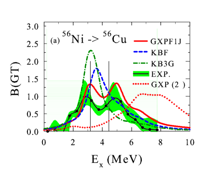
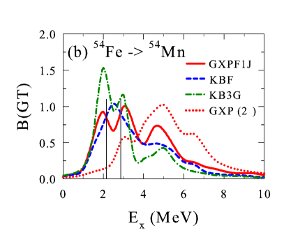
Figure 1: Comparison of the B(GT) strength function. (a) Three shell model calculations and experimental data for ⁵⁶Ni$\rightarrow^{56}$Cu (Sasano et al., 2012, 2011). (b) Three shell model calculations. Strengths from the 2⁺ states are also included. The vertical lines indicate the region where the KBF model is larger than the GXP model.

The shell-model calculations are carried out with the code MSHELL (Mizusaki, 2000), allowing at most five nucleons to be excited from the $0f_{7/2}$ orbit. The GT strength distributions are obtained by following the prescription of Whitehead (1980).

The GT strength functions for ⁵⁶Ni$\rightarrow^{56}$Cu and ⁵⁴Fe$\rightarrow^{54}$Mn are shown in Figure 1 for several shell model calculations compared to experimentally determined values (Sasano et al., 2012, 2011) for ⁵⁶Ni. For the intermediate excitation energy range at $\sim$4 MeV for the ⁵⁶Ni reaction, B(GT) drops in the experiment and in the GXPF1J model. However, this decrease does not appear for the KBF and KB3G models. The net result is an expected decrease in the EC rate on ⁵⁶Ni. While the GXPF1J results are not as low at $E_{x}\sim$4 MeV as the experimental results, the trend in this model is similar to that of the experimental results at this energy.

At higher energies ($E_{x}>$4 MeV), however, the value of B(GT) for the GXPF1J model exceeds those predicted by the KBF and KB3G models. This crossover (indicated by the vertical lines in Figure 1) above 4 MeV may be less significant as one convolves the strengths with the Fermi function and the electron energy distribution. Overall, the EC rates are expected to be lower for the GXPF1J model for a high-enough temperature.

For the ⁵⁴Fe reaction, the drop in B(GT) at $E_{x}\lesssim$ 4 MeV is less apparent depending on which KB parametrization is used. For the KB3G model, the the strength function for GXP is lower at $E_{x}\lesssim$ 3 MeV, and higher above this crossover energy. The GXP and KBF parametrizations are similar with a few deviations.

Also shown in Figure 1 are the strength functions for electron captures from the first excited state of the parent nucleus. These will be discussed in a later section. The EC rates of pf-shell nuclei are evaluated for GXPF1J by including contributions from all the excited states of parent nuclei up to $E_{x}$ = 2 MeV.

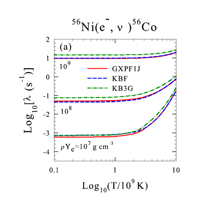
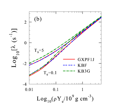
Figure 2: Electron capture rates for ⁵⁶Ni as a function of (a) temperature for various values of $\rho Y_{e}$ and (b) $\rho Y_{e}$ for various temperatures. Here $T_{9}\equiv T/(10^{9}~{}K$).

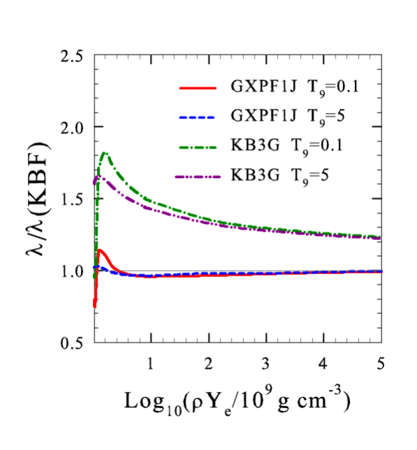
Figure 3: The ratio of the ⁵⁶Ni electron capture rate as a function of $\rho Y_{e}$ for various temperatures. The ratios for four models with respect to the KBF rates (Poves et al., 2001) are shown.

The resultant EC rates for ⁵⁶Ni are shown as a function of temperature and $\rho Y_{e}$ in Figure 2 comparing the GXPF1J, KBF, and KB3G models. Here $T_{9}\equiv T/(10^{9}~{}K)$. As expected, the KB3G model produces the highest rates overall at high temperatures and $\rho Y_{e}$. The difference between the KBF and the GXPF1J rates is smaller - a difference of about 10% in most cases. At higher temperatures, the difference between the KBF and GXPF1J rates diminishes. This is likely due to the fact that at higher temperatures, the spread in electron energies is higher as the Fermi function has a larger effective range. The integration of the rates over the larger span in electron energies results in an integration over a larger effective range of energies in B(GT). This integration would include the region where B(GT)${}_{KBF}>$B(GT)_GXPF1J and the region where B(GT)${}_{KBF}<$B(GT)_GXPF1J. These two effects would counteract each other.

A comparison of the reaction rates for the ⁵⁶Ni EC reaction is shown in Figure 3. Here, we take the ratio of several rate determinations to those of the KBF rates. Several shell model calculations for two temperatures as a function of $\rho Y_{e}$ are employed. It can be seen that the differences between a chosen shell model and the KBF are largest at low $\rho Y_{e}$. It is also noted that at higher temperatures, the rates in all models converge, as the electron energy distribution is integrated over a larger portion of B(GT). However, while the KB3G rates are larger than the KBF rates at low $Y_{e}$ by as much as $\sim$ 60%, the enhancement in rates for the GXP model is only about 10%, precluding a potentially small effect on Ni production in SNe Ia.

It is also noted from Figure 1 that the experimentally determined GT strengths for ⁵⁶Ni$\rightarrow^{56}$Cu exceed those determined using the GXPF1J and KBF models slightly for the energy range 1.5 $\lesssim E_{x}\lesssim$2.5 MeV. This region may be important for the production of ⁵⁶Ni in SNIa as the temperature drops significantly at this stage of the nucleosynthesis. A possible increase in EC rates for ⁵⁶Ni cannot be ruled out from the experimental data.

This point is further exemplified in Figure 4. Here, the ratio of GXP rates to KBF rates, $\lambda_{GXP}/\lambda_{KBF}$ are shown for 11 nuclei considered in Cole et al. (2012). This evaluation was performed for $T_{9}=3$ and $\rho Y_{e}=10^{7}$ g cm^-3. From here, no systematic trend is determined as the relationship between nuclear structure and the thermodynamic environment of a SN Ia is complex. The ratios are within 0.4-2.4, which shows that the e-capture GXP and KBF rates are close to each other - within a factor of 2.5. This is also true for Ga (Z=31) and Ge (Z=32). Effects from the use of the GXPF1J model for nuclei with Z=31 and 32 and 23$\leq Z\leq$30 are, therefore, expected to be modest at best.

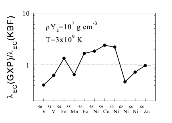
Figure 4: The ratios of electron capture rates from the GXP model to those of the KBF model for 11 nuclei compared in Cole et al. (2012).

3 Nucleosynthesis Calculations

To evaluate the effects of changes in capture rates on SN Ia nucleosynthesis, the two-dimensional electron-capture (EC) rates as a function of $\rho Y_{e}$ and temperature have been determined based on the GT strength functions to produce two nuclear reaction networks. The nuclear reaction networks used are summarized in Table 1. Two different rate tables were used in combination with two different SN Ia explosion scenarios modeled by their hydrodynamic trajectories.

Table 1: Summary of the nuclear reaction networks used in this study along with the rate tables and hydrodynamic explosion trajectories used (Nomoto, Thielemann, & Yokoi, 1984; Iwamoto et al., 1999).

Model	Explosion	$\lambda(Z<21)$	$\lambda(21\leq Z\leq 32)$
I	W7	Fuller, Fowler, & Newman (1982a, b); Oda et al. (1994)	KBF
II	W7	Fuller, Fowler, & Newman (1982a, b); Oda et al. (1994)	GXP
III	WDD2	Fuller, Fowler, & Newman (1982a, b); Oda et al. (1994)	KBF
IV	WDD2	Fuller, Fowler, & Newman (1982a, b); Oda et al. (1994)	GXP

The first network employed EC rates for the KBF model (Caurier et al, 1999; Langanke & Martínez-Pinedo, 2001) for proton-rich pf-shell nuclei with 21$\leq$Z$\leq$32 (for mass A, 45$\leq A\leq$ 65). The second network used rates computed from the GXP shell model for the same subset of nuclei. In both networks, for nuclei outside this region, the rates of Oda et al. (1994) were used for $sd$-shell nuclei while the rates of Fuller, Fowler, & Newman (1982a, b) were used otherwise. All other reaction rates were taken from the JINA REACLIB database (Cyburt et al., 2010). The libnucnet reaction network engine was used for the nucleosynthesis calculations (Meyer & Adams, 2007).

Both nuclear reaction networks were run using the hydrodynamics of the W7 deflagration (Nomoto, Thielemann, & Yokoi, 1984) and WDD2 delayed-detonation WD explosion model (Iwamoto et al., 1999). Trajectories for the deflagration and shock-front burning were followed. From this, an analysis and comparison of the production of pf-shell nuclei were done similar to that performed previously (Brachwitz et al., 2000; Iwamoto et al., 1999).

In this evaluation, the individual trajectories of the explosion models are decoupled from the nucleosynthesis and used as inputs in the nuclear reaction network. Each trajectory is a mass layer in the explosion. The electron chemical potential and electron fraction are computed implicitly at each time step for each trajectory and used as inputs in the weak rates. It is noted that while decoupling the reaction network from the explosion trajectories allows for a rapid evaluation of the effects of multiple shell models on the nucleosynthesis, the differences in heating induced by differences in the reaction rates is not accounted for. The uncertainty in this approximation will be discussed in the next section.

4 Results

Nuclear reaction network calculations were run for the central trajectories in the W7 deflagration and the WDD2 delayed-detonation explosion models (Iwamoto et al., 1999). The final abundances were computed based on these network calculations. Rates for pf-shell nuclei were computed for both the GXPF1J shell model and the KBF model (Langanke & Martínez-Pinedo, 2001). (Here, the reaction network results are referred to as the GXP and KBF models for networks using the GXPF1J and KBF shell models, respectively.)

4.1 Deflagration Model

As mentioned in §1 deflagration models, such as the W7 model(Nomoto, Thielemann, & Yokoi, 1984; Thielemann, Nomoto, & Yokoi, 1986), attempt to simulate the effects of increased nuclear burning because of an increase in the surface area of the flame front as it propagates to the stellar surface. The flame (deflagration) speed is prescribed by mixing-length theory. It accelerates to 0.08$c_{s}$ in t=0.6 sec and to 0.3$c_{s}$ in t=1.18 sec, where $c_{s}$ is the local sound speed (Nomoto, Thielemann, & Yokoi, 1984).

The deflagration model W7 was explored using networks I and II in Table 1. Here, the thermodynamic trajectories of Nomoto, Thielemann, & Yokoi (1984) have been used as inputs to the nuclear reaction network. The evolution of the electron fraction $Y_{e}$ is shown in Figure 5 for several trajectories in both models. The values of $Y_{e}$ at the end of the nucleosynthesis calculations ($t\approx 3.5$ s) are also shown in Table 2 for the same trajectories. In this figure, each line represents the evolution of a mass element for the W7 model assuming a specific shell model assumption. For all models, the electron fraction is lower near the core. It can be seen that the electron fraction changes little between the GXP and the KBF models indicating that, though the GXP shell model results in a significantly different B(GT), the net effects on the nucleosynthesis are potentially insignificant.

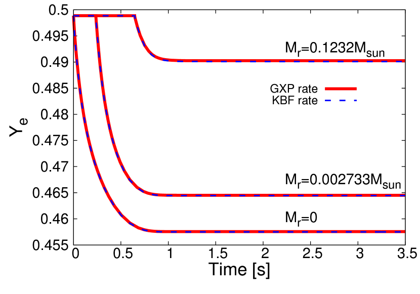
Figure 5: The evolution of the electron fraction for several trajectories in the GXP model (model II), given by the solid lines, and the KBF model (model I), given by the dashed line.

Table 2: The electron fractions at 3.5 s for the trajectories in Figure 5 for each shell model used in this paper. Roman numerals in parentheses indicate the model number indicated in Table 1.

	$M_{r}$=0	$M_{r}/M_{\odot}$=	$M_{r}/M_{\odot}$=
		0.002733	0.1232
GXP (II)	0.457555	0.464515	0.490261
KBF (I)	0.457501	0.464453	0.490101

Figure 6 shows the final mass fraction ratios for both calculations:

$$R\equiv\frac{X(Z,N)_{GXP}}{X(Z,N)_{KBF}}$$ (2)

Ratios are shown for the central trajectory (at a mass radius $M_{r}$=0) and an off-center trajectory (at $M_{r}$=0.1232$M_{\odot}$). It can be seen that the GXP model results in a more proton-rich final abundance distribution, but the effect is small. While this is not surprising as the electron capture rates are lower in the pf-shell region for the GXP model, the overall increase in $Y_{e}$ (as seen in Figure 5) is small.

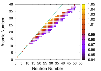
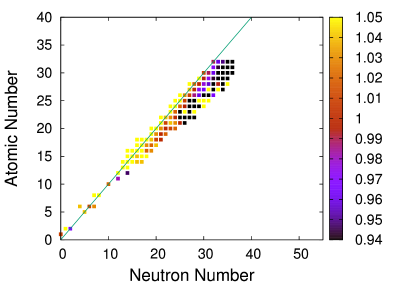
Figure 6: Abundance ratios $Y_{GXP}/Y_{KBF}$ at $t=3.5$s in the core, $M_{r}$=0 (left) and for the mass element located at $M_{r}$=0.1232$M_{\odot}$ (right) showing an abundance shift towards more proton-rich nuclei. The N=Z line is indicated in the plots.

It is also noted that the final abundances for the GXP model are more proton-rich for nuclei outside of the region where the rates differ. Of course, a reduction in the EC rates results in a global increase in $Y_{e}$, which will affect all electron capture rates. Thus, while the overall electron fraction may change only slightly, the final abundance distriubution for a particular species may change by a larger amount.

Using the final abundances for each trajectory in the W7 model, the final mass fraction profile has been determined. These profiles are shown in Figure 7 for the GXP model evaluated in this work. These mass fractions closely resemble those of prior work (Brachwitz et al., 2000).

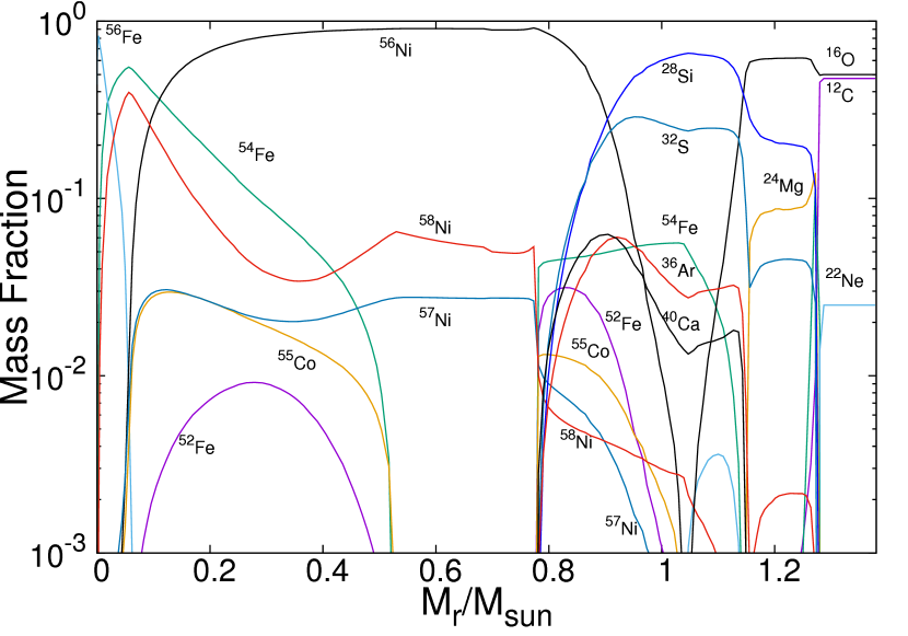
Figure 7: Isotopic distributions as a function of mass using the GXP rates (model II) at the end of the nucleosynthesis calculations($t=3.5$ s). The results for the KBF model are nearly identical.

From the final abundance ratios in each trajectory, a total abundance weighted by the mass of each trajectory is computed for the isotopes in the network - the overproduction factor. This double ratio, explicitly defined as:

$$DR\equiv\frac{{Y_{i}}/{Y_{Fe}}}{{Y_{i,\odot}}/{Y_{Fe,\odot}}}=\frac{Y_{i}/Y_{i,\odot}}{Y_{Fe}/Y_{Fe,\odot}}$$ (3)

provides a measure of the uniformity of the nucleosynthesis compared to solar observations. These double ratios are shown in Figure 8 for the GXP model. The ratios for the KBF model are nearly identical and comparable to the results of Brachwitz et al. (2000). Notable are the overabundances of ⁵⁸Ni compared to the production of lighter Z nuclei.

The nuclei ⁵⁴Mn and ⁵⁴Cr can also be addressed in Figure 8. Although a small fraction of ⁵⁴Cr is created from electron captures on ⁵⁴Mn, ⁵⁴Cr is produced in significant abundance in the inner 10${}^{-3}M_{\odot}$ of the model, where the electron fraction $Y_{e}<$ 0.46. Thus, while it is not seen in Figure 7 because the scaling of this figure is not fine enough, its production is still evident in Figure 8. It is not surprising that ⁵⁴Cr is produced in greatest abundance in the center mass shell as the $Y_{e}$ of this shell reaches a value very close to that of ⁵⁴Cr ($Y_{e}\sim Z/A=0.44$) as seen from Figure 5 and Table 2. From a nuclear statistical equilibrium (NSE) argument, one would expect this to be the mass shell with the largest final abundance of ⁵⁴Cr. This is also the mass shell with the lowest final $Y_{e}$. It is possible that an overall increase in $Y_{e}$ of the entire model by a small amount could result in dramatic changes in the ⁵⁴Cr production. This is because all of the mass shells above the central shell would have $Y_{e}$ which is even farther away from that of ⁵⁴Cr. If the $Y_{e}$ of the central shell increases to above 0.46 (a shift of less than 1%), then the overall ⁵⁴Cr production would start to decrease. However, production of nuclei with a higher $Y_{e}$, such as ⁵⁶Ni, would not be expected to decrease significantly because it is produced in a large range of mass shells with a range of electron fractions above and below that of ⁵⁶Ni ($Y_{e}\approx Z/A=0.5$). In the case of ⁵⁶Ni, while a single shell closer to the surface may produce less ⁵⁶Ni, shells below it would have an increased production, thus compensating for the loss. The inner mass shell has no shells below it, and any loss suffered by an overall increase in $Y_{e}$ could not be compensated for. Even more, a global shift of $Y_{e}$ for all shells may also increase the overall production of $\alpha$-cluster elements such as ²⁸Si.

For this reason, ⁵⁴Cr could be a good indicator of the effectiveness of the nucleosynthesis in a SN Ia as it is produced predominately in a small region of the star. Small global shifts, which tend to be averaged into multiple regions of the star, have more significant effects for the central region. Because of this, it is worthwhile to explore nucleosynthesis and thermodynamic effects such as turbulence and mixing within the SN Ia. In this case, 3D modeling - or 1D and 2D approximations - would become important.

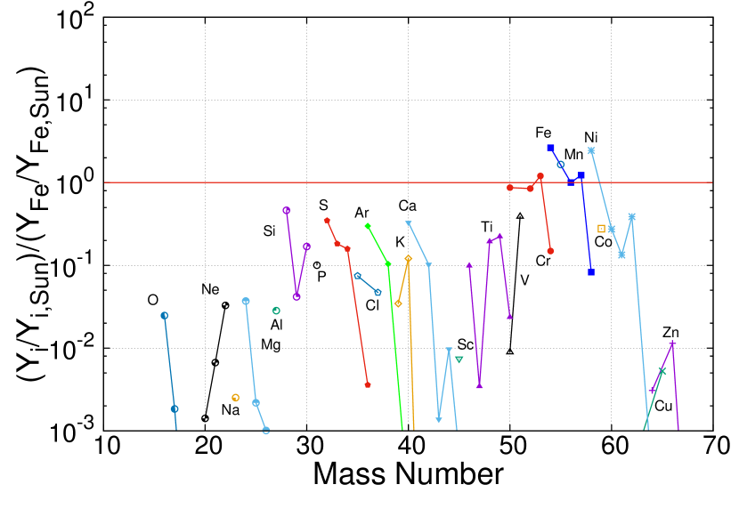
Figure 8: Deflagration (W7) final abundance ratios relative to Fe relative to the solar abundance ratio. The ratio is for the GXP model (model II), and results for the KBF model (model I) are nearly identical.

To compare the GXP and KBF models, we take a ratio of the abundances produced in each model weighted by the individual mass shells in the explosion. This ratio is shown in Figure 9. A small reduction of $\lesssim$5% is noted for the pf-shell nuclei with a slight increase in only a few cases. The production generally decreases in the GXP model for higher neutron number, consistent with a slight shift to higher $Y_{e}$ in the GXP model.

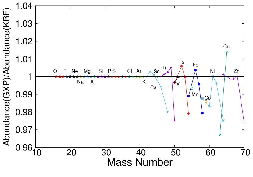
Figure 9: The ratio of abundances for nuclei produced in the GXP model (model II) to those of nuclei produced in the KBF model (model I). The results shown here are for the W7 deflagration model (Nomoto, Thielemann, & Yokoi, 1984).

Despite the seemingly significant differences in B(GT) between the GXP and KBF models, why are the differences in the nucleosynthesis so small (and likely unobservable)? The answer lies in the intersection of nuclear physics and the hydrodynamics of the deflagration model.

The total electron capture rate for a transition from a parent state to a daughter state is:

$$\lambda= \ln 2\frac{(g_{A}/g_{V})^{2}}{6143}\sum_{i}\frac{\left(2J_{i}+1\right)e^{-E_{i}/kT}}{G(Z,A,T)}\times$$ (4)

$$\sum_{j}{B_{ij}(GT)f_{ij}(T,\rho,\mu)}$$

where the sum is over transitions from parent to daughter states. The phase space factor, $f_{ij}$, accounts for the energetic feasibility of the reaction, including the population of electrons at a particular energy (Langanke & Martínez-Pinedo, 2000):

$$f_{ij} =\int_{\omega_{l}}^{\infty}\omega p\left(Q_{ij}+\omega\right)^{2}F(Z,\omega)S_{e}(T)$$ (5)

$$\times(1-S_{\nu}(Q_{ij}+\omega))d\omega$$

where $Q_{ij}$ is the electron capture transition energy divided by the electron mass, determined from the nuclear masses, and transitions are summed in Equation 4 from initial states $E_{i}$ to final states $E_{j}$. The distribution function is $S_{e,\nu}(\omega)$; here, $S_{e}$ is the usual Fermi-Dirac distribution, and $S_{\nu}=0$. The normalized total electron energy (kinetic plus rest mass) is $\omega=E_{e}/m_{e}c^{2}$. Coulomb barrier penetration effects are contained within the function $F(Z,\omega)$. The integration limits are set by the reaction threshold $\omega_{l}$, which is the threshold value for which EC is energetically feasible; $\omega_{l}=1$ if $Q_{ij}>-1$ and $\omega_{l}=\left|Q_{ij}\right|$ for $Q_{ij}<-1$. For $Q_{ij}<-1$, the electron must have enough kinetic energy to make the reaction possible, and $\omega_{l}>1$. An electron with zero kinetic energy will not exceed the reaction threshold.

We consider the case of electron captures on ⁵⁴Fe. The ground-state to ground-state Q-value for ⁵⁴Fe EC (using nuclear masses) is $-$1.21 MeV, meaning that to integrate over the strength function shown in Figure 1, the electron must have a total energy of at least 1.21 MeV. This raises the integration threshold in Equation 5. In order for the Fermi distribution $S_{e}(T)$ to have a population with the electron energy above the threshold $\omega>\omega_{l}$, either the density must be high enough to push the Fermi energy above the threshold, or the temperature must be hot enough so that the smearing of the Fermi surface creates a population of electrons above threshold, or both.

However, during the nucleosynthesis, the time at which the production of ⁵⁴Fe is reached does not occur until about 0.5 s in the mass shell which has the largest mass fraction of Fe by the end of the nucleosynthesis, corresponding to a mass of $5.612\times 10^{-2}M_{\odot}$. By this time, the temperature has dropped significantly in the W7 model, and the Fermi energy is less than 1.5 MeV. The spread in the Fermi surface is roughly 1 MeV, so nearly all electrons have energies less than 2 MeV. This means that the sum over B(GT) in Figure 1 is only at excitation energies less than 2 MeV. One sees from Figure 1 that the differences between the KBF and GXP strength functions are small in this region. This is indicated in Figure 10 which shows the integrated strength functions vs. the excitation energy of the daughter nucleus. For electron captures on ⁵⁴Fe, only excitation energies less than 2 MeV are important, in a region where the KBF and GXP strengths are nearly equal.

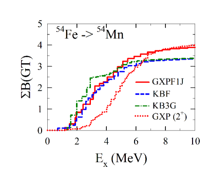
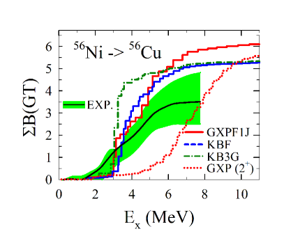
Figure 10: Integrated GT strengths vs. excitation energy for the three models compared in this paper. Left: ⁵⁴Fe. Right: ⁵⁶Ni along with experimental values. Also shown in each figure are the sums for EC transitions from the first excited state in the parent nuclei.

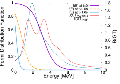
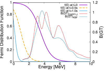
Figure 11: Fermi distributions for mass shells that produce the largest amount of ⁵⁶Ni (left) and ⁵⁴Fe (right) for three different times in the mass shell evolution. The distributions are shown with the B(GT) strengths for both nuclei. The B(GT) strengths have been shifted by the EC Q-value to show the electron energy necessary from each Fermi distribution to populate the specific excitation energy in the strength function. The thermodynamic trajectories are those of the deflagration model W7, corresponding to models I and II in this work.

The case is similar for electron captures on ⁵⁶Ni. Although the Q-value is positive for this reaction (1.622 MeV), the temperature and density by the time ⁵⁶Ni is reached in the nucleosynthesis are roughly the same as for ⁵⁴Fe. While a small population of electron energies exceeds 3 MeV where there is some deviation between the GXP and KBF models, most of the electron population exists at energies less than 1 MeV, corresponding to excitation energies less than 2.6 MeV, where the electron capture rates are low and the difference between the GXP and KBF strength functions is negligible. This can be seen by examining the integrated strength functions in Figure 10 in which deviations between the GXP and KBF models do not occur until excitation energies greater than about 3 MeV for ⁵⁶Ni with less deviation for ⁵⁴Fe except at very high excitation energies.

This is shown schematically in Figure 11. In this figure the GT strengths are shown for ⁵⁶Ni and ⁵⁴Fe for the KBF and GXPF1J shell models. Electron Fermi distributions for the mass shells that produce the largest amount of ⁵⁶Ni and ⁵⁴Fe are overlayed onto these figures for various times along the mass shell evolution. The GT strengths have been offset by the electron capture Q-value (ground state) in each case to provide an accurate picture of the actual electron energy necessary to reach a specific excited state in the daughter nucleus.

It is seen from this figure that while the mass shell starts off hot enough to create a population of electrons energetic enough to populate parts of the GT strength where the differences are significant between the two shell models, one must keep in mind that the nucleosynthesis path for each mass shell does not reach ⁵⁶Ni and ⁵⁴Fe until later in the shell evolution, in both cases about 0.5 s after the explosion starts. By this time, the mass shell has cooled to the point at which nearly the entire Fermi distribution lies in the energy region where the difference between the GXP and KBF strengths is insignificant as shown in the figure. Thus, the difference in EC rates for these two nuclei is small for these explosion models.

From Figures 8 and 9, it can be seen that the difference between the abundances determined using the GXP model and the KBF model are very small - on the order of a few percent. Furthermore, it can be seen that the abundance differences only exist at Z$>$19. By the time these nuclei are produced, the temperature of the environment is low and the nuclear abundances match those very close to an environment in NSE. Any heating from nucleosynthesis for Z$>$19 is not expected to differ significantly from that of the model of Iwamoto et al. (1999). Thus, the decoupling of the reaction network from the explosion trajectories is not expected to produce significant uncertainties.

4.2 Delayed-Detonation Model

Nucleosynthesis calculations were also carried out for the delayed-detonation model (Iwamoto et al., 1999) using models III and IV in Table 1. In this model, the explosion transitions from a deflagration near its center to a detonation at low density (Khokhlov, 1991). This particular model is parametrized by the transition density with the transition density parameter set to match observed light curves and nucleosynthesis.

In the delayed detonation, a slow deflagration phase is calculated by Nomoto, Thielemann, & Yokoi (1984) with an assumed constant flame speed of 0.015$c_{s}$. This is a typical laminar deflagration speed without convection and flame instabilities. The subsequent detonation (shock) phase is calculated by Iwamoto et al. (1999). It is assumed that DDT happens when the density at the flame front (upstream density) decreases to 2.2$\times$10⁷ g cm^-3.

Detailed nucleosynthesis calculations of delayed detonation models find that the problem of overproduction of neutron-rich isotopes may be remedied by constraining the density at which DDT occurs to $\sim 10^{7}$ g cm^-3 (Iwamoto et al., 1999; Brachwitz et al., 2000), which agrees with more physically based estimates (Bychkov & Liberman, 1995; Niemeyer & Woosley, 1997; Woosley, 2007). This is consistent with the results of multi-dimensional simulations of delayed detonation models (Seitenzahl et al., 2013).

As with the deflagration models (I and II), calculations were done assuming both a GXP and KBF shell model. The resulting mass fractions using the WDD2 hydrodynamic trajectories are shown in Figure 12. These mass fractions compare to those found using the W7 model of Iwamoto et al. (1999).

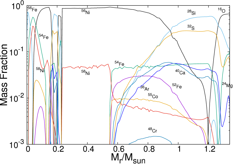
Figure 12: Same as Figure 7, but for the WDD2 delayed-detonation model.

Nuclear overproduction factors for nucleosynthesis using the GXP model (model IV) are compared to solar abundances in Figure 13. Compared to the W7 model (model II), the production of Cr, Mn, Fe, Ni, Cu, and Zn isotopes seems to match the solar distributions more closely across the isotopic chains studied, though the underproduction of Cu and Zn still exists.

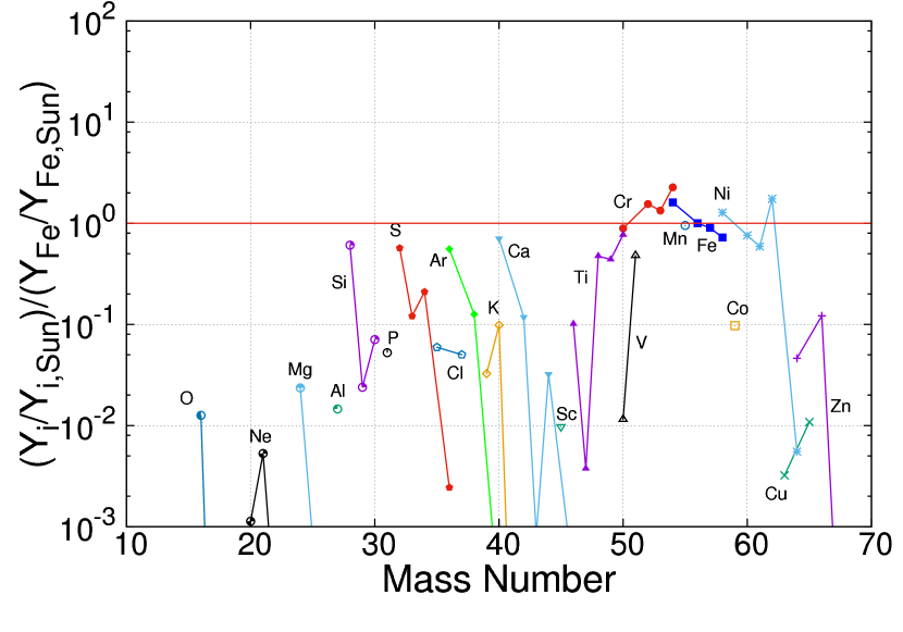
Figure 13: The ratio of abundances for nuclei produced in the GXP model for the WDD2 delayed-detonation model corresponding to model IV in Table 1.

As with the deflagration model, the GXP calculation is compared to a calculation done using KBF rates for the delayed-detonation model. The final abundance ratios are shown in Figure 14. The ratios are slightly closer to unity in this model than in the deflagration model, while the shapes are similar. This is an indicator that the delayed-detonation model is not as sensitive to rate changes as the deflagration model.

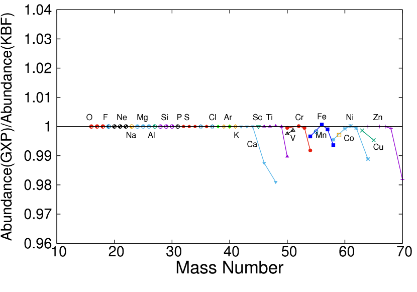
Figure 14: The ratio of abundances for nuclei produced in the GXP model to those of nuclei produced in the KBF model. The results shown here are for the WDD2 delayed-detonation model, comparing models III and IV in Table 1.

The explanation for these small differences between the GXP and KBF rates is the same as that given in the comparison of the deflagration model. That is, transitions in SNe Ia are only to low excitation energies as the Fermi energy of the electrons is $\sim$ 1 to 2 MeV. In this region, the differences between the GT strength functions are small.

A comparison of the total produced Fe and Ni mass is shown in Table 3 for all four models studied. One sees a slight shift to more ⁵⁶Fe production using the GXP shell model, corresponding to a very slight increase in $Y_{e}$ as indicated in Table 2.

Table 3: The total mass (in $M_{\odot}$) of ⁵⁶Fe and ⁵⁶Ni produced for each shell model and hydrodynamic model studied. Numbers in parentheses indicate the network-explosion model in Table 1.

	W7		WDD2
	GXP(II)	KBF(I)	GXP(IV)	KBF(III)
56Fe	0.66861	0.66631	0.68335	0.68291
56Ni	0.65142	0.64911	0.66812	0.66764

4.3 Nuclei in Excited States

Given the temperatures of the environments of SNe Ia, it is conceivable that nuclei in their excited states may result in reaction rates that vary from the ground-state rates. For this reason, it is worth mentioning the contribution to the EC rates for a few cases of nuclei in their excited states.

In Figure 1, the GT strength functions are shown in the GXP shell model for the first excited states of ⁵⁶Ni and ⁵⁴Fe, and the integrated strengths are shown in Figure 10. In both cases, the first excited state of the parent nucleus is the 2⁺ state. In each case, the strength function shifts to higher excitation energy. The shift of the strength from the excited 2⁺ states can be understood as a manifestation of the Brink hypothesis, which is primarily applicable to giant dipole resonances and can be applied to GT strength distributions. This hypothesis states that the giant dipole resonances (as well as the GT strengths) reside at the same energies relative to excited states as in the ground state (Axel, 1962; Misch, Fuller, & Brown, 2014; Guttormsen, 2016). While not exact, it can be used to understand the shift in the GT strengths in Figure 1. Details concerning the applicability of the Brink hypothesis have been discussed in Langanke & Martínez-Pinedo (2000). Detailed studies of the applicability of the Brink hypothesis for M1 strength functions are presented by Loens et al. (2012), Dzhioev et al. (2014), and Dzhioev et al. (2010). Thus, the shift of the strength function is commensurate with the excitation energy of the parent nucleus. In the case of SNe Ia nucleosynthesis, this shift would likely not change the resultant nucleosynthesis. This is because the excited states of the parent nuclei, the 2⁺ state in both ⁵⁶Ni and ⁵⁴Fe, are at 2.7 MeV and 1.4 MeV respectively. At the temperatures of the Type Ia SN environment, these states are not expected to have a significant population, and can be dismissed as possible contributors to the strength distributions.

5 Discussion

We continue the current effort in modern nuclear astrophysics towards a more accurate description of SN Ia nucleosynthesis using GT strength functions which more closely match experimental results.

Recent measurements of the GT strength distributions - used in determining EC rates - of pf-shell nuclei have called into question the validity of the theoretical distributions, which are important in determining nucleosynthesis in SNe Ia (Sasano et al., 2011, 2012).

A comparison was made between the GT strength functions B(GT) of the commonly used KBF model (Caurier et al, 1999) and the GXP models (Suzuki et al., 2011). It was found that the GXP shell model more closely matches the experimental B(GT) for ⁵⁶Ni (Sasano et al., 2011).

Using these strength distributions to determine EC rates for the pf-shell nuclei with 23$\leq{Z}\leq$30, nucleosynthesis in a type Ia SN was calculated using the thermodynamic trajectories of the deflagration model W7 (Nomoto, Thielemann, & Yokoi, 1984) and the delayed-detonation model WDD2 (Iwamoto et al., 1999). Comparisons of production were made between the W7 and WDD2 models for rates computed using the GXP and KBF shell model parametrizations.

While the GXP shell model results in rates which tend to shift the resultant nucleosynthesis to higher $Y_{e}$, thus increasing the Ni/Fe ratio, this shift is small, changing yields in the pf-shell region by only a few percent at best. Even though B(GT) is dramatically different in each shell model calculation, resulting in potentially significant rate changes as shown in Figure 4, the overall change in rates is also a function of the electron Fermi distribution, which depends on the environmental temperature. By the time the nucleosynthesis reaches the pf-shell nuclei, the temperature is low enough that the electron Fermi energy is about 1.5 MeV. Integrating over B(GT) in Figure 1 (while also taking the EC Q-value into account) results in a very small difference between the resultant rates since the integration is only over small transition energies, and the values of $E_{x}$ reached in the GT strength distributions are small, where the deviation between shell models is insignificant.

Excited states for ⁵⁶Ni and ⁵⁴Fe have also been investigated, with a corresponding shift in the GT strength distribution. Nuclei in excited states may shift the EC Q-values, and the shift in the GT strengths (a manifestation of the Brink-Axel hypothesis) may result in a slight reduction of the EC rates. However, it is noted that the excited states of doubly-magic ⁵⁶Ni and singly-magic ⁵⁴Fe in this regime are high enough that there will likely be little population of these states in a SN Ia. This should be studied in greater detail, however, as odd-A or odd-odd nuclei may have lower excited states with more significant populations in SNe Ia.

It’s also worth noting that because the GXP model is developed for pf-shell nuclei, application of a shell model with interactions which give different GT strengths to nuclei of lower mass, where the temperature of the SN Ia environment is hotter, may result in more significant changes in the nucleosynthesis. While type II supernovae are primarily responsible for production of these elements, SNe Ia are responsible for some of their production as well (Iwamoto et al., 1999). If the significant differences between the KBF and GXP models are at higher energies as suggested by the studies of ⁵⁶Ni and ⁵⁴Fe, then low-mass nuclei may exhibit a more pronounced change in abundance as they are produced earlier in the nucleosynthesis when the temperatures are hotter.

Finally, the importance of ⁵⁴Cr as a signature of the nucleosynthesis within the innermost mass shell is mentioned. This nucleus, with a Z/A=0.44, is one of the more proton-rich nuclei produced in the network calculations. As such, it is only produced in any significant abundance in the mass shells that have the lowest $Y_{e}$ distributions. However, if the $Y_{e}$ distribution is shifted globally over the entire star, then the production of ⁵⁴Cr may be altered dramatically. Any change to the central mass element (with the lowest $Y_{e}$) could have relatively large effects on the global production of ⁵⁴Cr. It may be worthwhile to examine this nucleus in greater detail and its sensitivity to the nuclear physics and stellar physics inputs.

In addition to ⁵⁴Cr, it may be worthwhile to investigate ⁵⁷Co and ⁵⁵Fe as signatures of the Chandra and sub-Chandra models. Recently, astronomers have detected radioactivity from ⁵⁷Co and ⁵⁵Fe (Shappee et al., 2016; Graur et al., 2016). If these can be shown to be sensitive to the central density, then verifications from astronomical observations may help to constrain the actual model used.

It is noted that corrections to EC rates for pf-shell nuclei relevant to SNe Ia using different nuclear shell models have resulted in smaller relative effects in the overall nucleosynthesis with historical changes decreasing with newer nuclear models. Because uncertainties in the nuclear physics are now apparently small, reducing the uncertainties in the stellar physics may provide larger corrections in the nucleosynthesis computations. Perhaps foremost among these would include an investigation of SNe Ia explosions in three dimensions. Also a systematic evaluation of the sensitivity of nuclear production to the uncertainties in the explosion may be worth pursuing. One example of such an exploration is the recent models in which the WD rotation is taken into account Benvenuto et al. (2015). In these models the central density is predicted to have a large variation and thus synthesis of neutron-rich Fe peak elements may be strongly affected. This also suggests the general importance of accurate electron capture rates for various conditions. Of course, uncertainties in nuclear physics relevant to other astrophysical scenarios, such as neutron-star crusts and type II supernovae, remain significant.

References

- Alford et al. (1991) Alford, W.P., et al. 1991, Nucl. Phys., A531, 97
- Alford et al. (1993) Alford, W. P., et al. 1993 Phys. Rev. C, 48, 2818
- Anantaraman et al. (2008) Anantaraman, N., et al. 2008, Phys. Rev. C, 78, 065803
- Arnett (1996) Arnett, D. 1996, Supernovae and Nucleosynthesis: An Investigation of the History of Matter from the Big Bang to the Present, Princeton: Princeton University Press
- Arnett (1979) Arnett, W.D. 1979, ApJ, 230, L37
- Arnett & Livne (1994) Arnett, D., & Livne, E. 1994, ApJ, 427, 315
- Axel (1962) Axel, P. 1962, Phys. Rev. 126, 671
- Bäumer et al. (2003) Bäumer, C., et al. 2003 Phys. Rev. C, 68, 031303(R)
- Bäumer et al. (2005) Bäumer,C., et al. 2005, Phys. Rev. C, 71, 024603
- Benvenuto et al. (2015) Benvenuto, O.G., Panei, J.A., Nomoto, K., Kitamura, H., & Hachisu, I. 2015, ApJL, 809, L6.
- Blinnikov & Khokhlov (1986) Blinnikov, S.I., & Khokhlov, A.M. 1986, Sov. Astron. Lett., 12, 131
- Boyd (2008) Boyd, R.N. 2008, An Introduction to Nuclear Astrophysics, Chicago: The University of Chicago Press
- Brachwitz et al. (2000) Brachwitz, F., Dean, D.J., Hix, W.R., Iwamoto, K., Langanke, K., Martínez-Pinedo, G., Nomoto, K., Strayer, M.R., Thielemann, F.-K., & Umeda, H. 2000, ApJ 536,934
- Branch et al. (1985) Branch, D., Doggett, J.B., Nomoto, K., & Thielemann, F.-K. 1985, ApJ, 294, 619
- Bychkov & Liberman (1995) Bychkov, V., & Liberman, M.A. 1995, A&A, 302, 727
- Caurier et al (1999) Caurier, E., Langanke, K., Martinez-Pinedo, G., & Nowacki, F. 1999, Nuc. Phys. A 653, 439
- Caurier et al. (2005) Caurier, E., Martinez-Pinedo, G., Nowacki, F., Poves, A., & Zuker, A.P. 2005, Rev. Mod. Phys. 77, 427
- Cole et al. (2006) Cole, A.L., et al. 2006, Phys. Rev. C, 74,034333
- Cole et al. (2012) Cole, A.L., Anderson, T.S., Zegers, R.G.T., Austin, S.M., Brown, B.A., Valdez, L., Gupta, S., Hitt, G.W., & Fawwaz, O. 2012, Phys. Rev. C 86, 015809
- Cyburt et al. (2010) Cyburt, R.H., Amthor, A.M., Ferguson, R., Meisel, Z., Smith, K., Warren, S., Heger, A., Hoffman, R.D., Rauscher, T., & Sakharuk, A. 2010, ApJS 189, 1
- Dzhioev et al. (2010) Dzhioev, A.A., Vdovin, A.I., Ponomarev, V.Y., Wamabch, J., Langanke, K., & Martínez-Pinedo, G. 2010, Phys. Rev. C, 81, 015804
- Dzhioev et al. (2014) Dzhioev, A.A., Vdovin, A.I., Wambach, J., & Ponomarev, V.Y. 2014, Phys. Rev. C, 89, 035805
- Fuller, Fowler, & Newman (1982a) Fuller, G.M., Fowler, W.A., & Newman, M.J. 1982, ApJ 252, 715
- Fuller, Fowler, & Newman (1982b) Fuller, G.M., Fowler, W.A., & Newman, M.J. 1982, ApJS 48, 279
- Gamezo, Khokhlov, & Oran (2005) Gamezo, V.N., Khokhlov, A.M., & Oran, E.S. 2005, ApJ623, 337
- Graur et al. (2016) Graur, O., Zurek, D., Shara, M.M. et al. 2016, ApJ, 819, 31
- Grewe et al. (2008) Grewe, E.W., et al. 2008, Phys. Rev. C, 77, 064303
- Guttormsen (2016) Guttormsen, M., Larsen, A.C., Gorgen, A., Renstrom, T., Siem, S., Tornyi, T.G., & Tveten, G.M. 2016, Phys. Rev. Lett. 116, 012502
- Hagemann et al. (2004) Hagemann, M., et al. 2004, Phys. Lett. B, 579, 251
- Hagemann et al. (2005) Hagemann, M., et al. 2005, Phys. Rev. C, 71, 014606
- Hillebrandt & Niemeyer (2000) Hillebrandt, W. & Niemeyer, J.C. 2000, ARA&A, 38, 191
- Hitt et al. (2009) Hitt, G.W., et al. 2009, Phys. Rev. C, 80, 014313
- Höflich et al. (1996) Höflich, P. et al. 1996, ApJ, 472, L81
- Honma et al. (2004) Honma, M., Otsuka, T., Brown, B.A., & Mizusaki, T. 2004, Phys. Rev. C 69, 034335
- Honma et al. (2005) Honma, M., Otsuka, T., Mizusaki, T, Hjorth-Jensen, M, & Brown, B.A. 2005, J. Phys. Conf. Ser., 20, 7
- Hoyle & Fowler (1960) Hoyle,F. & Fowler, W.A. 1960, ApJ, 132, 565
- Iben & Tutukov (1984) Iben, I.I. & Tutukov, A.V. 1984, ApJ, 284, 719
- Illiadis (2008) Illiadis, C. 2008, Nuclear Physics of Stars, John Wiley & Sons, Inc.
- Iwamoto et al. (1999) Iwamoto, K., Brachwitz, F., Nomoto, K., Kishimoto, N., Umeda, H., Hix, W.R., Thielemann, F.-K. 1999, ApJS, 125, 439
- Khokhlov (1991) Khokhlov, A.M. 1991, A&A, 245, 114
- Khokhlov (1995) Khokhlov, A.M. 1995, ApJ, 449, 695
- Kobayashi, Nomoto, & Hachisu (2015) Kobayashi, C., Nomoto, K., & Hachisu, I. 2015, ApJL, 804, L24
- Langanke & Martínez-Pinedo (2000) Langanke, K., & Martínez-Pinedo, G. 2000 NPA, 673, 481 (2000)
- Langanke & Martínez-Pinedo (2001) Langanke, K., & Martínez-Pinedo, G. 2001, At. Data Nucl. Data Tables 79, 1
- Langanke & Martínez-Pinedo (2003) Langanke, K. & Martínez-Pinedo, G. 2003, Rev. Mod. Phys., 75, 819
- Loens et al. (2012) Loens, H.P., Langanke, K., Martínez-Pinedo, G., & Sieja, K. 2012 Eur. Phys. J. A, 48, 34
- Maoz, Mannucci, & Nelemans (2014) Maoz, D., Mannucci, F., & Nelemans, G. 2014, ARA&A, 52, 107
- Maeda et al. (2010) Maeda, K., Taubenberger, S., Sollerman, J, et al. 2010, ApJ, 708, 1703
- Meyer & Adams (2007) Meyer, B.S. & Adams, D.C. 2007, Meteor. and Plan. Sci. Suppl. 2007, 5215
- Misch, Fuller, & Brown (2014) Misch, G.W., Fuller, G.M., & Brown B.A. 2014, Phys. Rev. C 90, 065808
- Mizusaki (2000) Mizusaki, T. 2000, RIKEN Accel. Prog. Rep., 33, 14
- Müller & Arnett (1982) Müller,D., & Arnett, W.D. 1982, ApJ, 261, L109
- Niemeyer & Woosley (1997) Niemeyer, J.C., & Woosley, S.E. 1997, ApJ, 475, 740
- Nomoto, Iwamoto, & Suzuki (1995) Nomoto, K., Iwamoto, K., & Suzuki, T. 1995, Phys.Rep., 256, 173
- Nomoto, Kamiya, & Nakasato (2013) Nomoto, K., Kamiya, Y., & Nakasato, N. 2013, in IAU Symposium 281 “Binary Paths to Type Ia Supernova Explosions”, 253 (ed. R. Di Stefano et al.) arXiv:1302.3371
- Nomoto, Kobayashi, & Tominaga (2013) Nomoto, K., Kobayashi, C., & Tominaga, N. 2013, ARAA, 51, 457
- Nomoto, Sugimoto, & Neo (1976) Nomoto, K., Sugimoto, D., & Neo, S. 1976, Ap&SS, 39, L37
- Nomoto, Thielemann, & Yokoi (1984) Nomoto, K., Thielemann, F.-K., & Yokoi, K. 1984, ApJ 286, 644
- Oda et al. (1994) Oda, T., Hino, M., Muto, K., Takahara, M., & Sato, K. 1994, ADANDT 56, 231
- Pakmor et al. (2013) Pakmor, R., Kromer, M., Taubenberger, S., et al. 2013, ApJL, 770, 8
- Parrent, Friesen, & Parthasarathy (2014) Parrent, J., Friesen, B., & Parthasarathy, M. 2014, Ap&SS, 351, 1
- Patat et al. (1996) Patat, F. et al. 1996, MNRAS, 278, 111
- Perlmutter et al. (1999) Perlmutter, S., et al. et al. 1999, ApJ, 517, 565
- Popescu et al. (2007) Popescu, L., et al. 2007, Phys. Rev. C, 75, 054312
- Riess et al. (1998) Riess, A.G., et al. 1998, AJ, 116, 1009
- Röpke et al. (2006) Röpke, F.K., Giesleler, M., Reinecke, M., Travaglio, C., & Hillebrandt, W. 2006, A&A 453, 260
- Poves et al. (2001) Poves, A., Sánchez-Solano, J., Caurier, E., & Nowacki, F. 2001, Nuc. Phys. A 694, 157
- Sasano et al. (2012) Sasano, M., Perdikakis, G., Zegers, R.G.T., Austin, S.M., Bazin, D., Brown, B.A., Ceasar, C., Cole, A.L., Deaven, J.M., Ferrante, N., Guess, C.J., Hitt, G.W., Meharchand, R., Montes, F., Palardy, J., Prinke, A., Riley, L.A., Sakai, H., Scott, M., Stolz, A., Valdez, L., & Yako, K. 2012, Phys. Rev. C 86, 034324
- Sasano et al. (2011) Sasano, M., Perdikakis, G., Zegers, R.G.T., Austin, S.M., Bazin, D., Brown, B.A., Ceasar, C., Cole, A.L., Deaven, J.M., Ferrante, N., Guess, C.J., Hitt, G.W., Meharchand, R., Montes, F., Palardy, J., Prinke, A., Riley, L.A., Sakai, H., Scott, M., Stolz, A., Valdez, L., & Yako, K. 2011, Phys. Rev. Lett. 107, 202501
- Sato et al. (2016) Sato, Y., Nakasato, N., Tanikawa, A. et al. 2016, ApJ, 821, 67
- Schmidt et al. (2008) Schmidt, W., Niemeyer, J.C., Hillebrandt, W., & Röpke, F.K. 2008, A&A, 450, 283
- Seitenzahl et al. (2013) Seitenzahl, I.R., et al. 2013, MNRAS, 429, 1156
- Shappee et al. (2016) Shappee, B.J., Stanke, K.Z., Kochanek, C.S., & Garnavich, P.M. 2016, arXiv:astroph/1608.01155
- Suzuki et al. (2011) Suzuki, T., Honma, M., Mao, H., Otsuka, T., & Kajino, T. 2011, Phys. Rev. C 83, 044619
- Thielemann, Nomoto, & Yokoi (1986) Thielemann, F.-K., Nomoto, K., & Yokoi, K. 1986, A&A, 158, 17
- Vetterli et al. (1987) Vetterli, M.C., et al. 1987, Phys. Rev. Lett., 59, 439
- Vetterli et al. (1989) Vetterli, M.C., et al. 1989, Phys. Rev. C, 40, 559
- von Neumann-Cosel et al. (1998) Von Neumann-Cosel, P., Poves, A., Retamosa, J., & Richter, A. 1998, Phys. Lett. B 443, 1
- Wang & Han (2012) Wang, B., & Han, Z. 2012, New Astron. Rev., 56, 122
- Webbink (1984) Webbink, R.F. 1984, ApJ, 277, 355
- Whitehead (1980) Whitehead, R.R. 1980, Moment Methods in Many Fermion Systems, edited by Dalton,. B.J. et al.
- Williams et al. (1995) Williams, A.L, et al. 1995, Phys. Rev. C 51, 1144
- Woosley (2007) Woosley, S.E. 2007, ApJ, 668, 1109
- Yako et al. (2009) Yako, K., et al. 2009, Phys. Rev. Lett., 103, 012503
- Yamaguchi et al. (2015) Yamaguchi, H., Badenes, C., Foster, A.R., et al. 2015, ApJL, 801, L31