A Bivariate Spline Method for Second Order Elliptic Equations in Non-Divergence Form

Abstract

A bivariate spline method is developed to numerically solve second order elliptic partial differential equations (PDE) in non-divergence form. The existence, uniqueness, stability as well as approximation properties of the discretized solution will be established by using the well-known Ladyzhenskaya-Babuska-Brezzi (LBB) condition. Bivariate splines, discontinuous splines with smoothness constraints are used to implement the method. A plenty of computational results based on splines of various degrees are presented to demonstrate the effectiveness and efficiency of our method.

1 Introduction

We are interested in developing an efficient numerical method for solving second order elliptic equations in non-divergence form. To this end, consider the model problem: Find $u=u(x)$ satisfying

(1.1) $$\sum_{i,j=1}^{2}a_{ij}\partial_{ij}^{2}u+cu =f,\quad\mbox{in }\Omega,$$

(1.2) $$u =0,\quad\mbox{on }\partial\Omega,$$

where $\Omega$ is an open bounded domain in $\mathbb{R}^{2}$ with a Lipschitz continuous boundary $\partial\Omega$, $\partial_{ij}^{2}$ is the second order partial derivative operator with respect to $x_{i}$ and $x_{j}$ for $i,j=1,2$. Assume that the tensor $a(x)=\{a_{ij}(x)\}_{2\times 2}$ is symmetric positive definite and uniformly bounded over $\Omega$, the coefficient $c(x)$ is non-positive and uniformly bounded over $\Omega$. In addition, we assume that the coefficients $a_{ij}(x)$ are essentially bounded so that the second order model problem (1.1) cannot be rewritten in a divergence form which many existing numerical methods can be employed to solve.

For convenience, we shall assume that the model problem (1.1) has a unique strong solution $u\in H^{2}(\Omega)$ satisfying the $H^{2}$ regularity:

(1.3) $$\|u\|_{H^{2}(\Omega)}\leq C\|f\|_{L^{2}(\Omega)}$$

for a positive constant $C$. Particularly, when $\Omega$ is a convex domain with $C^{2}$ smooth boundary, one can show that there exists a strong solution $u\in H^{2}(\Omega)$ of (1.1) satisfying the $H^{2}$ regularity (1.3) if the coefficient $c(x)\equiv 0$ and the coefficients $a_{ij}(i,j=1,2)$ satisfy the Cordés condition (cf. [18]):

(1.4) $$\frac{\sum_{i,j=1}^{2}a_{ij}^{2}}{(\sum_{i=1}^{2}a_{ii})^{2}}\leq\frac{1}{1+\epsilon},\qquad\text{in}\quad\Omega,$$

for a positive number $\epsilon\in(0,1]$. This condition is reasonable in $\mathbb{R}^{2}$ in the sense that when the coefficient tensor $a(x)$ satisfies the standard uniform ellipticity, i.e., there exist two positive numbers $\lambda_{1}$ and $\lambda_{2}$ such that

(1.5) $$\lambda_{1}\xi^{\top}\xi\leq\xi^{\top}a(x)\xi\leq\lambda_{2}\xi^{\top}\xi,\quad\forall\xi\in\mathbb{R}^{2},x\in\Omega,$$

then the Cordés condition holds true in $\mathbb{R}^{2}$ (cf. [18]). Indeed, when $c\equiv 0$, the existence of the unique strong solution $u$ satisfying (1.3) can be found in [18] based on a contraction map argument. Recently, in [20], the researchers weakened the assumption on the $C^{2}$ smooth boundary and use the well-known Lax-Milgram theorem to establish the weak solution to (1.1) with $c\equiv 0$ when $\Omega$ is convex with Lipschitz differentiable boundary $\partial\Omega$. In fact, as the solution $u\in H^{2}(\Omega)$, the weak solution is the strong solution. It is easy to see that the proofs in [18] and [20] can be extended to establish the existence and uniqueness of the strong solution in $H^{2}(\Omega)$ for the PDE in (1.1) when $\Omega$ is convex as each convex domain automatically has Lipschitz differentiable boundary, i.e. $C^{1,1}$ boundary. Numerical approximations of $u$ using the discontinuous Galerkin (DG) method and the weak Galerkin (WG) method have been studied in [20] and [23] to solve (1.1) with $c\equiv 0$. The convergence and convergence rates of these two numerical methods were established together with numerical evidence of convergence over convex and nonconvex domains.

In this paper, our goal is to provide another efficient computational method for numerical solution of (1.1). More precisely, we propose a bivariate spline method based on the minimization of the jumps of functions across edges and the boundary condition. Bivariate splines are discontinuous piecewise polynomial functions which are written in Bernstein-Bézier polynomial form (cf. [16]) and the smoothness constraints across an edge $e$ of triangulation $\triangle$ are written in terms of the coefficients of polynomials over the two triangles sharing the edge $e$. In particular, smoothness conditions for any smoothness $r\geq 0$ across edges of any order are implemented in MATLAB which can be simply used. This is an improvement over the internal penalties in the DG method. Bivariate splines have been used for numerical solutions of various types of PDE. See [3], [17], [13], [2], [12], [19], and etc.. They can be very convenient for numerical solutions of this type of PDE. See an extensive numerical evidence in §6.

Note that in [20], an hp-version discontinuous Galerkin finite element method was proposed and analyzed. It was based on a variational form arising from testing the original PDE against the Laplacian of sufficiently smooth functions (e.g., twice differentiable functions in $L^{2}$). According to the researchers in [20], their method yielded an optimal order of convergence regarding to the mesh size $h$, i.e. $d-1$ for polynomial degree $d=2,3,4,5$. We use the same $C^{1}$ test function for a PDE with non-differentiable coefficients and provide an evidence that the convergence rate of $|u-S_{u}|_{H^{2}(\Omega)}$ using bivariate spline method is also $d-1$ for $d=5,6,7,8$ when $c\equiv 0$. In addition, we present numerical convergence of $u-S_{u}$ in $L^{2}$ norm and $H^{1}$ semi-norm which can be better than $d-1$ for various $d$. When $c\not=0$, we have the same convergence behavior. In particular, the convergence rate of $|u-S_{u}|_{H^{2}(\Omega)}$ is still $d-1$.

Also, it is worthy pointing out that the researchers in [23] proposed a primal-dual weak Galerkin finite element method for this type of PDE (i.e. $c\equiv 0$), yielding an optimal order error estimate in a discrete $H^{2}$-norm for the primal variable and in the $L^{2}$-norm for the dual variable, as well as a convergence theory for the primal variable in the $H^{1}$- and $L^{2}$-norms. Although the numerical method implemented in [23] works for finite element partitions consisting of arbitrary polygons or polyhedra, only polynomials of degree 2 over triangulation were implemented and used for numerical solution. The flexibility of using bivariate splines of various degrees make our method more convenient to increase the accuracy of solutions. More accurate numerical solutions than the ones in [23] are presented in this paper to demonstrate the advantage of our bivariate spline method.

The theoretical study in this paper uses the same assumptions as in [23] and extend their arguments in [23] to analyze the PDE in (1.1) with nonzero $c$ and the convergence of the bivariate spline method. Our analysis in this paper is significantly different from that for discontinuous Galerkin method in [20]. The paper is organized as follows: We first start with an explanation of the primal-dual discontinuous Galerkin method to solve (1.1) in the next section. Mainly, we establish some basic properties such as the existence, uniqueness, stability of the method in Section 3. Then in Section 4 we present an error analysis of the numerical solution. Next we reformulate the primal-dual discontinuous Galerkin algorithm based on the bivariate spline functions and explain our implementation based on bivariate splines explained in [3]. Extensive numerical results are reported in Section 6. We start with a PDE with smooth coefficients and test on a smooth solution to demonstrate that the bivariate spline method works very well. For comparison purpose, we use the PDE in (1.1) with $c\equiv 0$. Then we apply the bivariate spline method to numerically solve a few PDE with non-differentiable coefficients and non-smooth solutions as well as $c\not=0$. Our method is able to approximate the nonsmooth solution very well. Therefore, the bivariate spline method is effective and efficient.

2 A Primal-Dual Discontinuous Galerkin Scheme

Our model problem seeks for a function $u\in H^{2}(\Omega)$ satisfying $u|_{\partial\Omega}=0$ and

(2.1) $$(\sum_{i,j=1}^{2}a_{ij}\partial_{ij}^{2}u+cu,w)=(f,w),\qquad\forall w\in L^{2}(\Omega).$$

Let ${\cal T}_{h}$ be a polygonal finite element partition of the domain $\Omega\subset\mathbb{R}^{2}$. Denote by ${\mathcal{E}}_{h}$ the set of all edges in ${\cal T}_{h}$ and ${\mathcal{E}}_{h}^{0}={\mathcal{E}}_{h}\setminus\partial\Omega$ the set of all interior edges. Assume that ${\cal T}_{h}$ satisfies the shape regularity conditions described in [5, 24]. Denote by $h_{T}$ the diameter of $T\in{\cal T}_{h}$ and $h=\max_{T\in{\cal T}_{h}}h_{T}$ the mesh size of the partition ${\cal T}_{h}$. Let $k\geq 0$ be an integer. Let $P_{k}(T)$ be the space of polynomials of degree no more than $k$ on the element $T\in{\cal T}_{h}$.

For any given integer $k\geq 2$, we define the finite element spaces composed of piecewise polynomials of degree $k$ and $k-2$, respectively; i.e.,

$$X_{h}=\{u:u|_{T}\in P_{k}(T),\quad\forall T\in{\cal T}_{h}\},$$

$$M_{h}=\{u:u|_{T}\in P_{k-2}(T),\quad\forall T\in{\cal T}_{h}\}.$$

Denote by ${[\![v]\!]}$ the jump of $v$ on an edge $e\in{\mathcal{E}}_{h}$; i.e.,

(2.2) $$\begin{split}{[\![v]\!]}=\left\{\begin{array}[]{ll}v|_{T_{1}}-v|_{T_{2}},&e=(\partial T_{1}\cap\partial T_{2})\subset{\mathcal{E}}_{h}^{0},\\ v,&e\subset\partial\Omega,\end{array}\right.\end{split}$$

where $v|_{T_{i}}$ denotes the value of $v$ as seen from the element $T_{i}$, $i=1,2$. The order of $T_{1}$ and $T_{2}$ is non-essential in (2.2) as long as the difference is taken in a consistent way in all the formulas. Analogously, one may define the jump of the gradient of $u$ on an edge $e\in{\mathcal{E}}_{h}$, denoted by ${[\![\nabla u]\!]}$.

For any $v\in X_{h}$, the quadratic functional $J(v)$ is given by

(2.3) $$\begin{split}J(v)=&\frac{1}{2}\sum_{e\in{\cal E}_{h}}h_{T}^{-3}\langle{[\![v]\!]},{[\![v]\!]}\rangle_{e}+\frac{1}{2}\sum_{e\in{\cal E}_{h}^{0}}h_{T}^{-1}\langle{[\![\nabla v]\!]},{[\![\nabla v]\!]}\rangle_{e}.\end{split}$$

It is clear that $J(v)=0$ if and only if $v\in C^{1}(\Omega)\cap X_{h}$ with the homogeneous Dirichlet boundary data $v=0$ on $\partial\Omega$.

We introduce a bilinear form

(2.4) $$b_{h}(v,q)=\sum_{T\in{\cal T}_{h}}(\sum_{i,j=1}^{2}a_{ij}\partial_{ij}^{2}v+cv,q)_{T},\quad\forall v\in X_{h},\ \forall q\in M_{h}.$$

The numerical solution of the model problem (1.1)-(1.2) can be characterized a constrained minimization problem as follows: Find $u_{h}\in X_{h}$ such that

(2.5) $$u_{h}=\operatorname*{arg~{}min}_{v\in X_{h},\ b_{h}(v,q)=(f,q),\ \forall q\in M_{h}}J(v).$$

By introducing the following bilinear form

(2.6) $$s_{h}(u,v)=\sum_{e\in{\cal E}_{h}}h_{T}^{-3}\langle{[\![u]\!]},{[\![v]\!]}\rangle_{e}+\sum_{e\in{\cal E}_{h}^{0}}h_{T}^{-1}\langle{[\![\nabla v]\!]},{[\![\nabla v]\!]}\rangle_{e},\quad\forall u,v\in X_{h},$$

the constrained minimization problem (2.5) has an Euler-Lagrange formulation that gives rise to a system of linear equations by taking the Fréchet derivative. The Euler-Lagrange formulation for the constrained minimization algorithm (2.5) gives the following numerical scheme.

Algorithm 2.1.

(Primal-Dual Discontinuous Galerkin FEM) A numerical approximation of the second order elliptic problem (1.1)-(1.2) seeks to find $(u_{h};\lambda_{h})\in X_{h}\times M_{h}$ satisfying

(2.7) $$s_{h}(u_{h},v)+b_{h}(v,\lambda_{h}) = 0,\ \ \ \ \qquad\forall v\in X_{h},$$

(2.8) $$b_{h}(u_{h},q) = (f,q),\qquad\forall q\in M_{h}.$$

3 Existence, Uniqueness and Stability

In this section, we will derive the existence, uniqueness, and stability for the solution $(u_{h};\lambda_{h})$ of the primal-dual discontinuous Galerkin scheme (2.7)-(2.8).

For each element $T\in{\cal T}_{h}$, let $B_{T}$ be the largest disk inside of $T$ centered at $c_{0}$ with radius $r$ and $F_{k,B_{T}}(f)$ be the averaged Taylor polynomial of degree $k$ for $f\in L^{1}(T)$ (see page 4 of [16] for details). Note that the averaged Taylor polynomial $F_{k,B_{T}}(f)$ satisfies (cf. Lemma 1.5 in [16])

(3.1) $${\partial_{ij}^{2}F_{k,B_{T}}(f)}=F_{k-2,B_{T}}({\partial_{ij}^{2}f})$$

if $\partial_{ij}f\in L^{1}(T)$. Let $P_{X_{h}}(f)$ and $P_{M_{h}}(f)$ be interpolations/projections of $f$ onto the spaces $X_{h}$ and $M_{h}$ defined by $P_{X_{h}}(f)|_{T}=F_{k,B_{T}}(f)$ and $P_{M_{h}}(f)|_{T}=F_{k-2,B_{T}}(f)$ on each element $T\in{\cal T}_{h}$, respectively. Using (3.1) gives rise to

(3.2) $${\partial_{ij}^{2}P_{X_{h}}(f)}=P_{M_{h}}({\partial_{ij}^{2}f}),$$

on each element $T\in{\cal T}_{h}$,

Lemma 1.

[16] The interpolant operators $P_{X_{h}}$ and $P_{M_{h}}$ are bounded in $L^{2}(\Omega)$. In other words, for any $f\in L^{2}(\Omega)$ we have

(3.3) $$\|P_{X_{h}}(f)\|\leq C\|f\|,$$

(3.4) $$\|P_{M_{h}}(f)\|\leq C\|f\|,$$

where $C$ is a constant depending only on the shape parameter $\theta_{{\cal T}_{h}}=\max_{T\in{\cal T}_{h}}\frac{h_{T}}{\rho_{T}}$, $\rho_{T}$ is the radius of the largest inscribed circle of $T$.

Recall that ${\cal T}_{h}$ is a shape-regular finite element partition of the domain $\Omega$. For any $T\in{\cal T}_{h}$ and $\phi\in H^{1}(T)$, the following trace inequality holds true:

(3.5) $$\|\phi\|^{2}_{\partial T}\leq C(h_{T}^{-1}\|\phi\|_{T}^{2}+h_{T}\|\nabla\phi\|_{T}^{2}).$$

Deonte by $Q_{k-2}$ the $L^{2}$ projection onto the finite element space $M_{h}$. We introduce a semi-norm in the finite element space $X_{h}$, denoted by ${|||}\cdot{|||}$; i.e.,

(3.6) $${|||}v{|||}=\Big{(}\sum_{T\in{\cal T}_{h}}\|Q_{k-2}(\sum_{i,j=1}^{2}a_{ij}\partial^{2}_{ij}v+cv)\|_{T}^{2}+s_{h}(v,v)\Big{)}^{\frac{1}{2}},\qquad v\in X_{h}.$$

The following result shows that ${|||}\cdot{|||}$ defined in (3.6) is indeed a norm on $X_{h}$ when the meshsize $h$ is sufficiently small.

Lemma 2.

Assume that the $H^{2}$ regularity (1.3) holds true for the model problem (1.1)-(1.2), and that the coefficient tensor $a(x)=\{a_{ij}(x)\}_{2\times 2}$ and $c(x)$ are uniformly piecewise continuous in $\Omega$ with respect to the finite element partition ${\cal T}_{h}$. Then, there exists an $h_{0}>0$ such that ${|||}\cdot{|||}$ in (3.6) defines a norm on $X_{h}$ when the meshsize $h$ is sufficiently small such that $h\leq h_{0}$.

Proof.

It suffices to verify the positivity property for ${|||}\cdot{|||}$. To this end, note that for any $v\in X_{h}$ satisfying ${|||}v{|||}=0$ we have $s_{h}(v,v)=0$. It follows that ${[\![v]\!]}=0$ on each edge $e\in{\mathcal{E}}_{h}$ and ${[\![\nabla u]\!]}=0$ on each interior edge $e\in{\mathcal{E}}_{h}^{0}$. Hence, $v\in C^{1}(\Omega)$ and $v=0$ on $\partial\Omega$. In addition, on each element $T\in{\cal T}_{h}$, we have

$$Q_{k-2}(\sum_{i,j=1}^{2}a_{ij}\partial^{2}_{ij}v+cv)=0.$$

Thus,

$$\sum_{i,j=1}^{2}a_{ij}\partial^{2}_{ij}v+cv =(I-Q_{k-2})(\sum_{i,j=1}^{2}a_{ij}\partial^{2}_{ij}v+cv):=F.$$

Using the $H^{2}$-regularity assumption (1.3), there exists a constant $C$ such that

(3.7) $$\|v\|_{2}\leq C\|F\|.$$

Note that $a_{ij}(x)$ and $c(x)$ are uniformly piecewise continuous in $\Omega$ with respect to the finite element partition ${\cal T}_{h}$. Let $\bar{a}_{ij}$ and $\bar{c}$ be the average of $a_{ij}$ and $c$ on each element $T\in{\cal T}_{h}$. Then, for any $\varepsilon>0$, there exists a $h_{0}>0$ such that

$$\|a_{ij}-\bar{a}_{ij}\|_{L^{\infty}(\Omega)}\leq\varepsilon,\qquad\|c-\bar{c}\|_{L^{\infty}(\Omega)}\leq\varepsilon,$$

if the meshsize $h$ is sufficiently small such that $h\leq h_{0}$. Denote by $\bar{c}$ and $\bar{v}$ the average of $c$ and $v$ on each element $T\in{\cal T}_{h}$, respectively. It follows from the linearity of the projection $Q_{k-2}$ that

$$\begin{split}\|F\|\leq&\sum_{i,j=1}^{2}|a_{ij}-\bar{a}_{ij}|\|\partial^{2}_{ij}v\|+\sum_{i,j=1}^{2}\|Q_{k-2}((a_{ij}-\bar{a}_{ij})\partial^{2}_{ij}v)\|\\ &+\|(I-Q_{k-2})(cv-\bar{c}\bar{v})\|\\ \leq&C\varepsilon\|v\|_{2}+\|cv-\bar{c}\bar{v}\|\\ \leq&C\varepsilon\|v\|_{2}+\|(c-\bar{c})v+\bar{c}(v-\bar{v})\|\\ \leq&C\varepsilon\|v\|_{2}+C\varepsilon\|v\|+Ch\|v\|_{1}\\ \leq&C\varepsilon\|v\|_{2}+Ch\|v\|_{2},\end{split}$$

where we have used the boundedness of the $L^{2}$ projection $Q_{k-2}$, which, combined with (3.7), gives

$$\|v\|_{2}\leq C(\varepsilon+h)\|v\|_{2}.$$

This yields that $v=0$ as long as $\varepsilon$ is sufficiently small such that $C\varepsilon<1$, which can be easily achieved by adjusting the parameter $h_{0}$. This completes the proof of the lemma. ∎

We are now in a position to establish an inf-sup condition for the bilinear form $b_{h}(\cdot,\cdot)$.

Lemma 3.

(inf-sup condition) Under the assumptions of Lemma 2, for any $q\in M_{h}$, there exists a $v_{q}\in X_{h}$ such that

(3.8) $$b_{h}(v_{q},q) \geq \beta\|q\|^{2},$$

(3.9) $${|||}v_{q}{|||} \leq C\|q\|,$$

provided that the meshsize $h$ is sufficiently small.

Proof.

Consider an auxiliary problem that seeks $w\in H^{2}(\Omega)\cap H_{0}^{1}(\Omega)$ satisfying

(3.10) $$\sum_{i,j=1}^{2}a_{ij}\partial^{2}_{ij}w+cw=q,\qquad\text{in}\ \Omega.$$

From the regularity assumption (1.3), it is easy to know that the problem (3.10) has one and only one solution, and furthermore, the solution satisfies the $H^{2}$ regularity property; i.e.,

(3.11) $$\|w\|_{2}\leq C\|q\|.$$

By letting $v_{q}=P_{X_{h}}(w)$, from (3.2) we obtain

$$\partial^{2}_{ij}v_{q}=\partial^{2}_{ij}P_{X_{h}}(w)=P_{M_{h}}(\partial^{2}_{ij}w).$$

Letting ${\bar{a}}_{ij}$ be the average of $a_{ij}$ over $T\in{\cal T}_{h}$, we arrive at

$$\sum_{i,j=1}^{2}a_{ij}\partial^{2}_{ij}v_{q}+cv_{q}$$

$$= \sum_{i,j=1}^{2}\{(a_{ij}-{\bar{a}}_{ij})P_{M_{h}}(\partial^{2}_{ij}w)+P_{M_{h}}({\bar{a}}_{ij}\partial^{2}_{ij}w)\}+(c-\bar{c})P_{X_{h}}(w)+P_{X_{h}}(\bar{c}w)$$

$$= \sum_{i,j=1}^{2}\{(a_{ij}-{\bar{a}}_{ij})P_{M_{h}}(\partial^{2}_{ij}w)+P_{M_{h}}(({\bar{a}}_{ij}-a_{ij})\partial^{2}_{ij}w)+P_{M_{h}}(a_{ij}\partial^{2}_{ij}w)\}$$

$$+(c-\bar{c})P_{X_{h}}(w)+P_{X_{h}}((\bar{c}-c)w)+P_{X_{h}}(cw)$$

$$= \sum_{i,j=1}^{2}\{(a_{ij}-{\bar{a}}_{ij})P_{M_{h}}(\partial^{2}_{ij}w)+P_{M_{h}}(({\bar{a}}_{ij}-a_{ij})\partial^{2}_{ij}w)\}+(c-\bar{c})P_{X_{h}}(w)$$

$$+P_{X_{h}}((\bar{c}-c)w)+P_{M_{h}}(\sum_{i,j=1}^{2}a_{ij}\partial^{2}_{ij}w+cw)+P_{X_{h}}(cw)-P_{M_{h}}(cw)$$

$$= E_{T}+q+P_{X_{h}}(cw)-P_{M_{h}}(cw).$$

where we have used (3.10) and $P_{M_{h}}q=q$. Here, $E_{T}=\sum_{i,j=1}^{2}\{(a_{ij}-{\bar{a}}_{ij})P_{M_{h}}(\partial^{2}_{ij}w)+P_{M_{h}}(({\bar{a}}_{ij}-a_{ij})\partial^{2}_{ij}w)\}+(c-\bar{c})P_{X_{h}}(w)+P_{X_{h}}((\bar{c}-c)w)$.

With the above chosen $v_{q}$ as $P_{X_{h}}(w)$, we have

(3.12) $$\begin{split}b_{h}(v_{q},q)&=\sum_{T\in{\cal T}_{h}}(\sum_{i,j=1}^{2}a_{ij}\partial^{2}_{ij}P_{X_{h}}(w)+cP_{X_{h}}(w),q)_{T}\\ &=\sum_{T\in{\cal T}_{h}}(E_{T},q)_{T}+\|q\|^{2}+\sum_{T\in{\cal T}_{h}}(P_{X_{h}}(cw)-P_{M_{h}}(cw),q)_{T}.\end{split}$$

Note that the coefficient tensor $a(x)=\{a_{ij}\}_{2\times 2}$ and $c(x)$ are uniformly piecewise continuous over ${\cal T}_{h}$. Thus, for any given suifficiently small $\varepsilon>0$, we have $\|a_{ij}-{\bar{a}}_{ij}\|_{L^{\infty}(\Omega)}\leq\varepsilon$ and $\|c-{\bar{c}}\|_{L^{\infty}(\Omega)}\leq\varepsilon$ for sufficiently small meshsize $h$. It then follows from the Cauchy-Schwarz inequality, (3.3) - (3.4), and the $H^{2}$ regularity property (3.11) that

$$\left|\sum_{T\in{\cal T}_{h}}(E_{T},q)_{T}\right|$$

$$\leq C\varepsilon\Big{(}\sum_{T\in{\cal T}_{h}}\sum_{i,j=1}^{2}\|P_{M_{h}}(\partial^{2}_{ij}w)\|_{T}^{2}\Big{)}^{\frac{1}{2}}\Big{(}\sum_{T\in{\cal T}_{h}}\|q\|_{T}^{2}\Big{)}^{\frac{1}{2}}+C\varepsilon\Big{(}\sum_{T\in{\cal T}_{h}}\sum_{i,j=1}^{2}\|\partial^{2}_{ij}w\|_{T}^{2}\Big{)}^{\frac{1}{2}}\Big{(}\sum_{T\in{\cal T}_{h}}\|q\|_{T}^{2}\Big{)}^{\frac{1}{2}}$$

$$+C\varepsilon\Big{(}\sum_{T\in{\cal T}_{h}}\|P_{X_{h}}w\|_{T}^{2}\Big{)}^{\frac{1}{2}}\Big{(}\sum_{T\in{\cal T}_{h}}\|q\|_{T}^{2}\Big{)}^{\frac{1}{2}}+C\varepsilon\Big{(}\sum_{T\in{\cal T}_{h}}\|w\|_{T}^{2}\Big{)}^{\frac{1}{2}}\Big{(}\sum_{T\in{\cal T}_{h}}\|q\|_{T}^{2}\Big{)}^{\frac{1}{2}}$$

$$\leq C\varepsilon\Big{(}\sum_{T\in{\cal T}_{h}}\sum_{i,j=1}^{2}\|\partial^{2}_{ij}w\|_{T}^{2}\Big{)}^{\frac{1}{2}}\|q\|+C\varepsilon\Big{(}\sum_{T\in{\cal T}_{h}}\|w\|_{T}^{2}\Big{)}^{\frac{1}{2}}\|q\|$$

$$\leq C\varepsilon\|w\|_{2}\|q\|\leq C\varepsilon\|q\|^{2},$$

and

$$\Big{|}\sum_{T\in{\cal T}_{h}}(P_{X_{h}}(cw)-P_{M_{h}}(cw),q)_{T}\Big{|}$$

$$\leq \Big{(}\sum_{T\in{\cal T}_{h}}\|P_{X_{h}}(cw-\bar{c}\bar{w})-P_{M_{h}}(cw-\bar{c}\bar{w})\|^{2}_{T}\Big{)}^{\frac{1}{2}}\Big{(}\sum_{T\in{\cal T}_{h}}\|q\|^{2}_{T}\Big{)}^{\frac{1}{2}}$$

$$\leq \Big{(}\sum_{T\in{\cal T}_{h}}\|cw-\bar{c}\bar{w}\|^{2}_{T}\Big{)}^{\frac{1}{2}}\Big{(}\sum_{T\in{\cal T}_{h}}\|q\|^{2}_{T}\Big{)}^{\frac{1}{2}}$$

$$\leq \Big{(}\sum_{T\in{\cal T}_{h}}\|(c-\bar{c})w+\bar{c}(w-\bar{w})\|^{2}_{T}\Big{)}^{\frac{1}{2}}\|q\|$$

$$\leq (C\varepsilon\|w\|+Ch\|w\|_{1})\|q\|$$

$$\leq C(\varepsilon+h)\|w\|_{2}\|q\|$$

$$\leq C(\varepsilon+h)\|q\|^{2},$$

where $\bar{c}$ and $\bar{w}$ are the average of $c$ and $w$ on each element $T\in{\cal T}_{h}$, respectively, $C$ is a generic constant independent of ${\cal T}_{h}$. Substituting the above estimate into (3.12) yields

$$b_{h}(v_{q},q)\geq(1-C(2\varepsilon+h))\|q\|^{2},$$

which leads to the estimate (3.8) when the meshsize $h$ is sufficiently small.

It remains to derive the estimate (3.9). To this end, recall that

(3.13) $${|||}v_{q}{|||}^{2}=\sum_{T\in{\cal T}_{h}}\|Q_{k-2}(\sum_{i,j=1}^{2}a_{ij}\partial^{2}_{ij}v_{q}+cv_{q})\|^{2}_{T}+s_{h}(v_{q},v_{q}).$$

Letting $v_{q}=P_{X_{h}}(w)$, the first term on the right-hand side of (3.13) can be bounded by using (3.2), (3.3) and (3.11) as follows:

(3.14) $$\begin{split}\sum_{T\in{\cal T}_{h}}\|Q_{k-2}(\sum_{i,j=1}^{2}a_{ij}\partial^{2}_{ij}v_{q}+cv_{q})\|^{2}_{T}&=\sum_{T\in{\cal T}_{h}}\|Q_{k-2}(\sum_{i,j=1}^{2}a_{ij}\partial^{2}_{ij}P_{X_{h}}(w)+cP_{X_{h}}(w))\|^{2}_{T}\\ &\leq\sum_{T\in{\cal T}_{h}}\sum_{i,j=1}^{2}\|a_{ij}P_{M_{h}}(\partial^{2}_{ij}w)\|_{T}+\|cP_{X_{h}}(w)\|^{2}_{T}\\ &\leq C\sum_{i,j=1}^{2}\|a_{ij}\|^{2}_{L^{\infty}(\Omega)}\sum_{T\in{\cal T}_{h}}\|\partial^{2}_{ij}w\|_{T}^{2}+C\|c\|^{2}_{L^{\infty}(\Omega)}\sum_{T\in{\cal T}_{h}}\|w\|_{T}^{2}\\ &\leq C\|q\|^{2}.\end{split}$$

As to the term $s_{h}(v_{q},v_{q})$ in (3.13), note that it is defined by (2.6) using the jump of $v_{q}$ on each edge $e\in{\cal E}_{h}$ plus the jump of $\nabla v_{q}$ on each interior edge $e\in{\cal E}_{h}^{0}$. For an interior edge $e\in{\cal E}_{h}^{0}$ shared by two elements $T_{1}$ and $T_{2}$, we have

$${[\![v_{q}]\!]}|_{e} = v_{q}|_{T_{1}\cap e}-v_{q}|_{T_{2}\cap e}$$

$$= P_{X_{h}}(w)|_{T_{1}\cap e}-P_{X_{h}}(w)|_{T_{2}\cap e}$$

$$= (P_{X_{h}}(w)|_{T_{1}\cap e}-w|_{e})+(w|_{e}-P_{X_{h}}(w)|_{T_{2}\cap e}).$$

It follows that

(3.15) $$\langle{[\![v_{q}]\!]},{[\![v_{q}]\!]}\rangle_{e}\leq 2\|P_{X_{h}}(w)|_{T_{1}\cap e}-w|_{e}\|_{e}^{2}+2\|P_{X_{h}}(w)|_{T_{2}\cap e}-w|_{e}\|_{e}^{2}.$$

Using the trace inequality (3.5), we have

$$\|P_{X_{h}}(w)|_{T_{1}\cap e}-w|_{e}\|_{e}^{2}\leq Ch_{T}^{-1}\|P_{X_{h}}(w)-w\|^{2}_{T_{1}}+Ch_{T}\|\nabla(P_{X_{h}}(w)-w)\|^{2}_{T_{1}}.$$

Analogously, the following holds true

$$\|P_{X_{h}}(w)|_{T_{2}\cap e}-w|_{e}\|_{e}^{2}\leq Ch_{T}^{-1}\|P_{X_{h}}(w)-w\|^{2}_{T_{2}}+Ch_{T}\|\nabla(P_{X_{h}}(w)-w)\|^{2}_{T_{2}}.$$

Substituting the last two inequalities into (3.15) yields

(3.16) $$\langle{[\![v_{q}]\!]},{[\![v_{q}]\!]}\rangle_{e}\leq C\sum_{i=1}^{2}\left(h_{T}^{-1}\|P_{X_{h}}(w)-w\|^{2}_{T_{i}}+Ch_{T}\|\nabla(P_{X_{h}}(w)-w)\|^{2}_{T_{i}}\right).$$

For boundary edge $e\subset\partial\Omega$, from $w|_{e\subset\partial\Omega}=0$ we have

$${[\![v_{q}]\!]}|_{e} = v_{q}|_{e}=P_{X_{h}}(w)|_{e}-w|_{e}.$$

Thus, the estimate (3.16) remains to hold true. Summing (3.16) over all the edges yields

(3.17) $$\begin{split}\sum_{e\in{\cal E}_{h}}h_{T}^{-3}\langle{[\![v_{q}]\!]},{[\![v_{q}]\!]}\rangle_{e}&\leq C\sum_{T\in{\cal T}_{h}}\left(h_{T}^{-4}\|P_{X_{h}}(w)-w\|^{2}_{T}+Ch_{T}^{-2}\|\nabla(P_{X_{h}}(w)-w)\|^{2}_{T}\right)\\ &\leq C\|w\|_{2}^{2}\end{split}$$

where we have used the estimate (4.3) with $m=1$ and $s=0,1$ in the last inequality. Combining (3.17) with the regularity estimate (3.11) gives rise to

(3.18) $$\sum_{e\in{\cal E}_{h}}h_{T}^{-3}\langle{[\![v_{q}]\!]},{[\![v_{q}]\!]}\rangle_{e}\leq C\|q\|^{2}.$$

A similar argument can be applied to yield the following estimate

(3.19) $$\sum_{e\in{\cal E}_{h}^{0}}h_{T}^{-1}\langle{[\![\nabla v_{q}]\!]},{[\![\nabla v_{q}]\!]}\rangle_{e}\leq C\|q\|^{2}.$$

We emphasize that the summation in (3.19) is taken over all the interior edges so that no boundary value for $\nabla w$ is needed in the derivation of the estimate (3.19). Combining (3.18) and (3.19) with $s_{h}(v_{q},v_{q})$ yields

$$s_{h}(v_{q},v_{q})\leq C\|q\|^{2},$$

which, together with (3.14), completes the derivation of the estimate (3.9). ∎

Lemma 4.

(Boundedness) The following inequalities hold true:

$$\begin{split}|s_{h}(u,v)|\leq&{|||}u{|||}{|||}v{|||},\qquad\forall u,v\in X_{h},\\ |b_{h}(v,q)|\leq&C{|||}v{|||}\|q\|,\qquad\forall v\in X_{h},q\in M_{h}.\end{split}$$

Proof.

It follows from the definition of $s_{h}(\cdot,\cdot)$, ${|||}\cdot{|||}$ and Cauchy-Schwarz inequality that for any $u,v\in X_{h}$, we have

$$\begin{split}|s_{h}(u,v)|=&\Big{|}\sum_{e\in{\cal E}_{h}}h_{T}^{-3}\langle{[\![u]\!]},{[\![v]\!]}\rangle_{e}+\sum_{e\in{\cal E}_{h}^{0}}h_{T}^{-1}\langle{[\![\nabla u]\!]},{[\![\nabla v]\!]}\rangle_{e}\Big{|}\\ \leq&\Big{(}\sum_{e\in{\cal E}_{h}}h_{T}^{-3}\langle{[\![u]\!]},{[\![u]\!]}\rangle_{e}\Big{)}^{\frac{1}{2}}\Big{(}\sum_{e\in{\cal E}_{h}}h_{T}^{-3}\langle{[\![v]\!]},{[\![v]\!]}\rangle_{e}\Big{)}^{\frac{1}{2}}\\ &+\Big{(}\sum_{e\in{\cal E}_{h}^{0}}h_{T}^{-1}\langle{[\![\nabla u]\!]},{[\![\nabla u]\!]}\rangle_{e}\Big{)}^{\frac{1}{2}}\Big{(}\sum_{e\in{\cal E}_{h}^{0}}h_{T}^{-1}\langle{[\![\nabla v]\!]},{[\![\nabla v]\!]}\rangle_{e}\Big{)}^{\frac{1}{2}}\\ \leq&s_{h}(u,u)^{\frac{1}{2}}s_{h}(v,v)^{\frac{1}{2}}\\ \leq&{|||}u{|||}{|||}v{|||}.\end{split}$$

Next from the definition of $b_{h}(\cdot,\cdot)$, ${|||}\cdot{|||}$, and Cauchy-Schwarz inequality that for any $v\in X_{h}$, $q\in M_{h}$, we have

$$\begin{split}|b_{h}(v,q)|=&\Big{|}\sum_{T\in{\cal T}_{h}}(\sum_{i,j=1}^{2}a_{ij}\partial_{ij}^{2}v+cv,q)_{T}\Big{|}\\ =&\Big{|}\sum_{T\in{\cal T}_{h}}(Q_{k-2}(\sum_{i,j=1}^{2}a_{ij}\partial_{ij}^{2}v+cv),q)_{T}\Big{|}\\ \leq&(\sum_{T\in{\cal T}_{h}}\|Q_{k-2}(\sum_{i,j=1}^{2}a_{ij}\partial_{ij}^{2}v+cv)\|_{T}^{2})^{\frac{1}{2}}(\sum_{T\in{\cal T}_{h}}\|q\|_{T}^{2})^{\frac{1}{2}}\\ \leq&{|||}v{|||}\|q\|.\end{split}$$

These complete the proof. ∎

Define the subspace of $X_{h}$ as follows:

$$\Xi_{h}=\{{v}\in X_{h}:\quad b_{h}(v,q)=0,\quad\forall{q}\in M_{h}\}.$$

Lemma 5.

(Coercivity) There exists a constant $\alpha$, such that

$$s_{h}(v,v)\geq\alpha{|||}v{|||}^{2},\qquad\forall v\in\Xi_{h}.$$

Proof.

For any $v\in\Xi_{h}$, we have

$$b_{h}(v,q)=0,\qquad\forall q\in M_{h}.$$

It follows from the definition of $b(\cdot,\cdot)$ in (2.4) that

$$0=b_{h}(v,q)=\sum_{T\in{\cal T}_{h}}(\sum_{i,j=1}^{2}a_{ij}\partial_{ij}^{2}v+cv,q)_{T}=\sum_{T\in{\cal T}_{h}}(Q_{k-2}(\sum_{i,j=1}^{2}a_{ij}\partial_{ij}^{2}v+cv),q)_{T},$$

which yields

$$Q_{k-2}(\sum_{i,j=1}^{2}a_{ij}\partial_{ij}^{2}v+cv)=0,$$

on each $T\in{\cal T}_{h}$ by letting $q=Q_{k-2}(\sum_{i,j=1}^{2}a_{ij}\partial_{ij}^{2}v+cv)$. This implies $s_{h}(v,v)={|||}v{|||}^{2}$, which completes the proof with $\alpha=1$. ∎

Using the abstract theory for the saddle-point problem developed by Babuska [4] and Brezzi [6], we arrive at the following theorem based on Lemmas 3 - 5.

Theorem 6.

The primal-dual discontinuous Galerkin finite element method (2.7)-(2.8) has a unique solution $(u_{h};\lambda_{h})\in X_{h}\times M_{h}$, provided that the meshsize $h<h_{0}$ holds true for a sufficiently small but fixed parameter $h_{0}>0$. Moreover, there exists a constant C such that the solution $(u_{h};\lambda_{h})$ satisfies

(3.20) $${|||}u_{h}{|||}+\|\lambda_{h}\|\leq C\|f\|.$$

4 Error Estimates

Let $(u_{h};\lambda_{h})\in X_{h}\times M_{h}$ be the approximate solution of the model problem (1.1) arsing from primal-dual discontinuous Galerkin finite element method (2.7)-(2.8). Note that $\lambda=0$ is the exact solution of the trival dual problem $b_{h}(v,\lambda)=0$ for all $v\in H^{2}(\Omega)$. Define the errors functions by

$$e_{h}=u_{h}-P_{X_{h}}u,\qquad\epsilon_{h}=\lambda_{h}-P_{M_{h}}\lambda.$$

Lemma 7.

The error functions $e_{h}$ and $\epsilon_{h}$ satisfy the following equations:

(4.1) $$s_{h}(e_{h},v)+b_{h}(v,\epsilon_{h})= -s_{h}(P_{X_{h}}u,v),\qquad\forall v\in X_{h},$$

(4.2) $$b_{h}(e_{h},p)= l_{u}(p),\qquad\quad\qquad\quad\forall p\in M_{h},$$

where $l_{u}(p)=\sum_{T\in{\cal T}_{h}}\sum_{i,j=1}^{2}(a_{ij}(I-P_{M_{h}})\partial_{ij}^{2}u,p)_{T}+\sum_{T\in{\cal T}_{h}}(c(I-P_{X_{h}})u,p)_{T}$.

Proof.

By subtracting $s_{h}(P_{X_{h}}u,v)$ from both sides of (2.7), we obtain

$$s_{h}(u_{h}-P_{X_{h}}u,v)+b_{h}(v,\lambda_{h}-0)=-s_{h}(P_{X_{h}}u,v),\qquad\forall v\in X_{h},$$

which completes the proof of (4.1).

Substracting $b_{h}(P_{X_{h}}u,p)$ from both sides of (2.8), it follows from (3.2) and (1.1) that

$$\begin{split}&b_{h}(u_{h},p)-b_{h}(P_{X_{h}}u,p)\\ =&(f,p)-b_{h}(P_{X_{h}}u,p)\\ =&(f,p)-\sum_{T\in{\cal T}_{h}}\sum_{i,j=1}^{2}(a_{ij}\partial_{ij}^{2}(P_{X_{h}}u)+cP_{X_{h}}u,p)_{T}\\ =&(f,p)-\sum_{T\in{\cal T}_{h}}\sum_{i,j=1}^{2}(a_{ij}P_{M_{h}}(\partial_{ij}^{2}u)+cP_{X_{h}}u,p)_{T}\\ =&(f,p)-\sum_{T\in{\cal T}_{h}}(\sum_{i,j=1}^{2}a_{ij}\partial_{ij}^{2}u+cu,p)_{T}-\sum_{T\in{\cal T}_{h}}\sum_{i,j=1}^{2}(a_{ij}(P_{M_{h}}-I)\partial_{ij}^{2}u,p)_{T}-\sum_{T\in{\cal T}_{h}}(c(P_{X_{h}}-I)u,p)_{T}\\ =&(f,p)-(f,p)-\sum_{T\in{\cal T}_{h}}\sum_{i,j=1}^{2}(a_{ij}(P_{M_{h}}-I)\partial_{ij}^{2}u,p)_{T}-\sum_{T\in{\cal T}_{h}}(c(P_{X_{h}}-I)u,p)_{T}\\ =&\sum_{T\in{\cal T}_{h}}\sum_{i,j=1}^{2}(a_{ij}(I-P_{M_{h}})\partial_{ij}^{2}u,p)_{T}+\sum_{T\in{\cal T}_{h}}(c(I-P_{X_{h}})u,p)_{T},\\ \end{split}$$

which completes the proof of (4.2). ∎

The equations (4.1) and (4.2) are called error equations for the primal-dual discontinuous Galerkin finite element scheme. This is a saddle point system for which Brezzi’s Theorem can be employed for the analysis of stability.

Lemma 8.

[5, 24] Let ${\cal T}_{h}$ be a finite element partition of $\Omega$ satisfying the shape regular assumption given in [5, 24]. Then, for any $0\leq s\leq 2$ and $1\leq m\leq k$, one has

(4.3) $$\sum_{T\in{\cal T}_{h}}h_{T}^{2s}\|u-P_{X_{h}}u\|^{2}_{s,T}\leq Ch^{2(m+1)}\|u\|^{2}_{m+1},$$

(4.4) $$\sum_{T\in{\cal T}_{h}}h_{T}^{2s}\|u-P_{M_{h}}u\|^{2}_{s,T}\leq Ch^{2(m-1)}\|u\|^{2}_{m-1}.$$

Theorem 9.

Assume that the coefficient tensor $a(x)=\{a_{ij}(x)\}_{2\times 2}$ and $c(x)$ are uniformly piecewise continuous in $\Omega$ with respect to the finite element partition ${\cal T}_{h}$. Let $u$ and $(u_{h};\lambda_{h})\in X_{h}\times M_{h}$ be the solutions of (1.1) and (2.7) - (2.8), respectively. Assume that the exact solution $u$ of (1.1) is sufficiently regular such that $u\in H^{k+1}(\Omega)$. There exists a constant $C$ such that

$${|||}u_{h}-P_{X_{h}}u{|||}+\|\lambda_{h}-P_{M_{h}}\lambda\|\leq Ch^{k-1}\|u\|_{k+1},$$

provided that the meshsize $h<h_{0}$ holds true for a sufficiently small, but fixed $h_{0}>0$.

Proof.

It follows from Lemmas 3 - 5 that the Brezzi’s stability conditions are satisfied for the saddle point problem (4.1)-(4.2). Thus, there exists a constant $C$ such that

(4.5) $${|||}e_{h}{|||}+\|\epsilon_{h}\|\leq C\Bigg{(}\sup_{v\in{X_{h}},v\neq 0}\frac{|-s_{h}(P_{X_{h}}u,v)|}{{|||}v{|||}}+\sup_{p\in M_{h},p\neq 0}\frac{|l_{u}(p)|}{\|p\|}\Bigg{)}.$$

Recall that

(4.6) $$\begin{split}&\sup_{v\in{X_{h}},v\neq 0}\frac{|-s_{h}(P_{X_{h}}u,v)|}{{|||}v{|||}}\\ \leq&\sup_{v\in{X_{h}},v\neq 0}\frac{|\sum_{e\in{\cal E}_{h}}h_{T}^{-3}\langle{[\![P_{X_{h}}u]\!]},{[\![v]\!]}\rangle_{e}|+|\sum_{e\in{\cal E}_{h}^{0}}h_{T}^{-1}\langle{[\![\nabla P_{X_{h}}u]\!]},{[\![\nabla v]\!]}\rangle_{e}|}{{|||}v{|||}}\\ \end{split}$$

As to the first term of the right-hand side of (4.6), from Cauchy-Schwarz inequality, trace inequality (3.5) and (4.3), we have

(4.7) $$\begin{split}|\sum_{e\in{\cal E}_{h}}h_{T}^{-3}&\langle{[\![P_{X_{h}}u]\!]},{[\![v]\!]}\rangle_{e}|\leq C\Big{(}\sum_{e\in{\cal E}_{h}}h_{T}^{-3}\|{[\![P_{X_{h}}u]\!]}\|^{2}_{e}\Big{)}^{\frac{1}{2}}\Big{(}\sum_{e\in{\cal E}_{h}}h_{T}^{-3}\|{[\![v]\!]}\|^{2}_{e}\Big{)}^{\frac{1}{2}}\\ \leq&C\Big{(}\sum_{e\in{\cal E}_{h}}h_{T}^{-3}(\|{[\![P_{X_{h}}u]\!]}-{[\![u]\!]}\|^{2}_{e}+\|{[\![u]\!]}\|^{2}_{e})\Big{)}^{\frac{1}{2}}{|||}v{|||}\\ \leq&C\Big{(}\sum_{T\in{\cal T}_{h}}h_{T}^{-4}\|{[\![P_{X_{h}}u-u]\!]}\|^{2}_{T}+h_{T}^{-2}\|{[\![P_{X_{h}}u-u]\!]}\|^{2}_{1,T}\Big{)}^{\frac{1}{2}}{|||}v{|||}\\ \leq&Ch^{k-1}\|u\|_{k+1}{|||}v{|||},\end{split}$$

where we used ${[\![u]\!]}=0$ as $u\in H^{2}(\Omega)\cap H_{0}^{1}(\Omega)$. Similarly, we have

(4.8) $$|\sum_{e\in{\cal E}_{h}^{0}}h_{T}^{-1}\langle{[\![\nabla P_{X_{h}}u]\!]},{[\![\nabla v]\!]}\rangle_{e}|\leq Ch^{k-1}\|u\|_{k+1}{|||}v{|||}.$$

Substituting (4.7)-(4.8) into (4.6), we have

(4.9) $$\sup_{v\in{X_{h}},v\neq 0}\frac{|-s_{h}(P_{X_{h}}u,v)|}{{|||}v{|||}}\leq Ch^{k-1}\|u\|_{k+1}.$$

From Cauchy-Schwarz inequality and (4.4), we obtain

(4.10) $$\begin{split}&\qquad\sup_{p\in M_{h},p\neq 0}\frac{|l_{u}(p)|}{\|p\|}\\ =&\sup_{p\in M_{h},p\neq 0}\frac{\Big{|}\sum_{T\in{\cal T}_{h}}\sum_{i,j=1}^{2}(a_{ij}(I-P_{M_{h}})\partial_{ij}^{2}u,p)_{T}\Big{|}}{\|p\|}+\sup_{p\in M_{h},p\neq 0}\frac{\Big{|}\sum_{T\in{\cal T}_{h}}(c(I-P_{X_{h}})u,p)_{T}\Big{|}}{\|p\|}\\ \leq&\sup_{p\in M_{h},p\neq 0}\frac{\Big{|}\|a_{ij}\|_{L^{\infty}(\Omega)}\Big{(}\sum_{T\in{\cal T}_{h}}\sum_{i,j=1}^{2}\|(I-P_{M_{h}})\partial_{ij}^{2}u\|^{2}_{T}\Big{)}^{\frac{1}{2}}\Big{(}\sum_{T\in{\cal T}_{h}}\|p\|^{2}_{T}\Big{)}^{\frac{1}{2}}\Big{|}}{\|p\|}\\ &+\sup_{p\in M_{h},p\neq 0}\frac{\Big{|}\|c\|_{L^{\infty}(\Omega)}\Big{(}\sum_{T\in{\cal T}_{h}}\|(I-P_{X_{h}})u\|^{2}_{T}\Big{)}^{\frac{1}{2}}\Big{(}\sum_{T\in{\cal T}_{h}}\|p\|^{2}_{T}\Big{)}^{\frac{1}{2}}\Big{|}}{\|p\|}\\ &\leq Ch^{k-1}\|u\|_{k+1}+Ch^{k+1}\|u\|_{k+1}\\ &\leq Ch^{k-1}\|u\|_{k+1}.\end{split}$$

Substituting (4.9) and (4.10) into (4.5) completes the proof. ∎

5 Bivariate Spline Implementation of Algorithm 2.1

We notice that $X_{h}$ is a discontinuous spline space of degree $k$ over a finite element partition ${\cal T}_{h}$ and $M_{h}$ is a discontinuous spline space of degree $k_{1}$, e.g. $k_{1}=k-2$ over ${\cal T}_{h}$. When ${\cal T}_{h}$ is a triangulation, these are spline spaces which have been thoroughly studied in [3] and [16]. In this paper, let us explain how to use these spline functions for numerical solution of the second order elliptic PDE (1.1). When ${\cal T}_{h}$ is a triangulation, spline functions use the Bernstein-Bézier representation as explained in [16]. That is, the prime-dual discontinuous Galerkin FEM method discussed in the previous sections can be reformulated by using the Bernstein-Bézier representation. The representation has several nice properties (cf. [16]): (1) the basis functions form a partition of unity, (2) the basis functions are nonnegative, and (3) the basis functions have explicit formulas for their derivatives, integration, their inner product, and triple product integration.

In the remaining of the paper, we use both $u\in X_{h}$ and its coefficient vector ${\bf u}$ in terms of Bernstein-Bézier representation to write a discontinuous spline function $u$. Similarly, we use both $q\in M_{h}$ and its coefficient vector ${\bf q}$. Most importantly, for any function $u\in X_{h}$, $u$ is a piecewise polynomial function of degree $k$ over ${\cal T}_{h}$, the jump function ${[\![u]\!]}$ over an interior edge $e$ of ${\cal T}_{h}$ can be rewritten by using the smoothness conditions between the coefficients of two polynomial pieces $u|_{T_{1}}$ and $u|_{T_{2}}$ on their common edge $e$ for triangles $T_{1},T_{2}\in{\cal T}_{h}$ which share $e$. See [10] and [16]. The smoothness conditions are linear and all these conditions over each interior edge can be expressed together by using $H{\bf u}=0$ as explained in [3], where $H$ is a rectangular and sparse matrix and ${\bf u}$ is the coefficient vector of $u$.

On the boundary of $\Omega$, $u$ has to satisfy the Dirichlet boundary condition which can be approximated by using a standard polynomial interpolation method, i.e., $u({\bf x})|_{e}=g({\bf x})$ for $k+1$ distinct points ${\bf x}\in e$, where $e$ is a boundary edge of ${\cal T}_{h}$. As $u$ is a polynomial on $e$, the interpolation condition $u({\bf x})|_{e}=g({\bf x})$ can be expressed by linear equations in terms of its coefficients. We put these linear equations for all boundary edges together and express them by $B{\bf u}={\bf g}$, where $B$ is a rectangular and sparse matrix and ${\bf g}$ is a vector consisting of the values of $g$ at the $k+1$ equally-spaced points over $e$ for all boundary edges $e\in\triangle$.

The PDE equation in (2.1) can be discretized by using Bernstein-Bézier representation as follows. We first approximate the right-hand side $f$ by discontinuous spline functions in $S_{f}\in M_{h}$. For example, we may choose $S_{f}$ to be the piecewise polynomial function which interpolates $f$ at the domain points on $T$ of degree $k_{1}$ for all triangle $T\in{\cal T}_{h}$, under the assumption that $f$ is a continuous function. For another example, we choose $S_{f}\in M_{h}$ such that for each triangle $T\in{\cal T}_{h}$,

(5.1) $$\int_{T}fqdxdy=\int_{T}S_{f}qdxdy,\quad\forall q\in{\cal P}_{k_{1}},$$

where ${\cal P}_{k_{1}}$ is the standard polynomial space of total degree $k_{1}$. It is easy to know that the problem (5.1) has a unique solution of $S_{f}|_{T}$. Thus, $S_{f}\in{\cal M}_{h}$ is well-defined. In fact, we have the following properties

(5.2) $$\|S_{f}\|\leq\|f\|\hbox{ and }\|S_{f}-f\|=\min_{s\in M_{h}}\|s-f\|.$$

Indeed, we have $\int_{T}|S_{f}|^{2}dxdy=\int_{T}fS_{f}dxdy$ for all $T\in{\cal T}_{h}$ and use Cauchy-Schwarz inequality to have the inequality in (5.2). The equality in (5.2) can be seen from the solution of the least squares problem in (5.1).

We compute the inner product integration on the right-hand of (2.1) exactly by using Theorem 2.34 in [16] and a triple inner product formula. That is, we have

$$\int_{\Omega}fqdxdy=\int_{\Omega}S_{f}qdxdy=\langle M{\bf f},{\bf q}\rangle,$$

where ${\bf f}$ is the coefficient vector of $S_{f}$, $M$ is called the mass matrix which is a blockly diagonal matrix and ${\bf q}$ is the coefficient vector of $q$.

Similarly, we approximate the coefficients $a_{ij}$ by discontinuous spline functions in another discontinuous spline space $S_{ij}\in L_{h}=S^{-1}_{1}({\cal T}_{h})$ of degree $1$, say piecewise linear interpolation of $a_{ij}$.

(5.3) $$\int_{T}a_{ij}\partial^{2}_{ij}uqdxdy\approx\int_{T}S_{i,j}\partial^{2}_{ij}uqdxdy,\quad\forall u\in{\cal P}_{k},q\in{\cal P}_{k-2}.$$

Once we have $S_{ij}$, we compute triple product integration on the left-hand side of (2.1). That is, $\int_{T}S_{ij}\partial_{ij}^{2}uqdxdy$ has an exact formula in terms of the coefficients of $S_{ij},u,$ and $q$. Thus we have

$$\int_{\Omega}\sum_{i,j=1}^{2}a_{ij}\partial^{2}_{ij}uqdxdy\approx\int_{\Omega}\sum_{i,j=1}^{2}S_{ij}\partial^{2}_{ij}uqdxdy=\langle K{\bf u},{\bf q}\rangle,$$

where $K$ is the stiffness matrix related to the PDE (1.1).

In order to have an equality in the above formula, we now use the standard $L^{2}$ projection $P_{M_{h}}$ which is defined by $P_{M_{h}}(v)\in M_{h}$ such that

(5.4) $$\langle P_{M_{h}}(v),q\rangle=\langle v,q\rangle,\forall q\in M_{h}.$$

Thus, we have

$$\int_{\Omega}\sum_{i,j=1}^{2}a_{ij}\partial^{2}_{ij}uqdxdy=\langle P(\sum_{i,j=1}^{2}a_{ij}\partial^{2}_{ij}u),q\rangle=\int_{\Omega}\sum_{i,j=1}^{2}P_{M_{h}}(a_{ij}\partial^{2}_{ij}u)qdxdy.$$

Since the the projection is linear, we can write

$$\int_{\Omega}\sum_{i,j=1}^{2}P_{M_{h}}(a_{ij}\partial^{2}_{ij}u)qdxdy=\langle K{\bf u},{\bf q}\rangle,$$

for a blockly diagonal matrix $K$ and for all $q\in M_{h}$. In this way, we obtain a discretized PDE equation: $\langle K{\bf u},{\bf q}\rangle=\langle M{\bf f},{\bf q}\rangle$ for all ${\bf q}\in\mathbb{R}^{d({\cal M}_{h})}$ or a linear system:

(5.5) $$K{\bf u}=M{\bf f}.$$

Note that both $M$ and $K$ can be computed in parallel.

In terms of the Berstein-Bézier representation, the bilinear forms in (2.6) and (2.4) can be rewritten as

(5.6) $$s(u,v)=h^{2}\langle H{\bf u},H{\bf v}\rangle+h^{2}\langle B{\bf u},B{\bf v}\rangle,\quad\forall u,v\in X_{h},$$

and

(5.7) $$b(u,q)=\langle K{\bf u},{\bf q}\rangle,\quad\forall u\in X_{h},q\in M_{h}.$$

With the above preparation, Algorithm 2.1 can be recast as follows.

Let us consider the following minimization problem for (2.1): Find ${\bf u}$ satisfying

(5.8) $$\min\frac{h^{2}}{2}(\|H{\bf u}\|^{2}+\|B{\bf u}-{\bf g}\|^{2}),\quad\hbox{subject to }K{\bf u}=M{\bf f}.$$

Note that the boundary condition is imposed by minimizing the error in an least-squares sense so that the boundary conditions do not need to be strictly enforced.

This minimization problem (5.8) can be reformulated by using Lagrange multiplier method as follows: let

(5.9) $$L({\bf u},\lambda)=\frac{h^{2}}{2}(\|H{\bf u}\|^{2}+\|B{\bf u}-{\bf g}\|^{2})+{\bf\lambda}^{\top}(K{\bf u}-M{\bf f}),$$

where ${\bf\lambda}$ is a Lagrange multiplier. Thus, the minimizer ${\bf u}^{*}$ of (5.8) satisfies (5.10). Hence, we have

Algorithm 5.1.

(The Primal-Dual Bivariate Spline Method) Find a vector pair $({\bf u}^{*},{\bf\lambda}^{*})\in\mathbb{R}^{d(X_{h})}\times\mathbb{R}^{d(M_{h})}$ satisfying

(5.10) $$\begin{cases}h^{2}\langle H{\bf u}^{*},H{\bf d}\rangle+h^{2}\langle B{\bf u},B{\bf d}\rangle+\langle\lambda^{*},K{\bf d}\rangle&=h^{2}\langle{\bf g},B{\bf d}\rangle,\qquad\forall{\bf d}\in\mathbb{R}^{d(X_{h})},\cr\langle{\bf q},K{\bf u}^{*}\rangle&=\langle{\bf q},M{\bf f}\rangle,\qquad\forall{\bf q}\in\mathbb{R}^{d(M_{h})},\end{cases}$$

where $d(X_{h})$ is the dimension of $X_{h}$ and $d(M_{h})$ is the dimension of $M_{h}$. In fact, $d(X_{h})=(k+1)(k+2)N({\cal T}_{h})/2$ and $d(M_{h})=(k_{1}+1)(k_{1}+2)N({\cal T}_{h})/2$ with $N({\cal T}_{h})$ being the number of triangles in ${\cal T}_{h}$. We shall denote by $u_{h}\in X_{h}$ the spline solution with coefficient vector ${\bf u}^{*}$ and similarly, $\lambda_{h}\in M_{h}$ with coefficient vector $\lambda^{*}$.

This Algorithm 5.1 will be implemented and numerically experimented in this paper.

6 Numerical Results based on Minimization (5.8)

We have implemented Algorithm 5.1 in MATLAB based on the spline function implementation method discussed in [3] which is completely different from the spline functions implemented in [19]. Our main driving code is given below.

[V,T]=mytriangulation(3); %input a triangulation.
k=5; % degree of spline functions in X_h, You can use any integer d\ge 2.
k1=d-2; %degree of spline functions in M_h.
caseNum=101; %this number is the number in the test function list g2.
%The following three lines generate 1 million points for computing the RMSE.
xmin =min(V(:,1)); xmax=max(V(:,1)); xscal=xmax-xmin;
ymin =min(V(:,2)); ymax=max(V(:,2)); yscal=ymax-ymin;
[X,Y]=meshgrid(xmin:xscal/1000:xmax,ymin:yscal/1000:ymax);
%The exact solution: values and its derivatives.
[Exact,Exactdx,Exactdy,Exactxx,Exactxy,Exactyy]=g2(X(:),Y(:),caseNum);
L=5; %Level of refinement.
k2=2; %degree of splines to approximate the PDE coefficients.
for i=1:L
 [V,T]=refine(V,T); %uniform refinement of triangulation (V, T).
 [E,TE,TV,EV,B] = tdata(V,T); %triangulation relations
 H0 = smoothness(V,T,k,0); %The function value continuity conditions
 H1 = smoothness1(V,T,k,1);%The function derivative continuity conditions
 H=[H0;H1]; %or simply use:   H=smoothness(V,T,d,1);
 M=mass(V,T,k1); %the mass matrix
[A,B,C,D,E] = bnetw2(V,T,k2,’weights4PDE2’,caseNum);
%spline approximation of PDE coefficients above and  the weighted stiff matrices
[Kxx,Kxy,Kyx,Kyy,Kc]=bending2(V,T,k,k1,k2,A,B,C,D,E);
 K=Kxx+Kxy+Kyx+Kyy; %use K for simplicity.
 F = bnet2(V,T,k1,’ellipticPDE’,caseNum); %spline for the right-hand side of PDE
 [G,Bm] = dirchlet(V,T,TE,E,k,’g2’,caseNum); %generating the boundary conditions
%The following 3 lines are parameters for constrained iterative minimization.
 m = (k+1)*(k+2)/2; n = size(T,1);
 p1 = length(G); p2 = size(H,2);
 tol=1.0e-16;    eps=6;    max_it=5;
%The following CImin is an algorithm explained in Appendix 1.
    c=CImin(H’*H+Bm’*Bm,K’-Kc’,Bm’*G,M*F,eps,max_it, tol); %
% We now evaluate the spline approximation of the solution:
 s{1}=V;s{2}=T;s{3}=c; %s is a spline of coefficients c over triangulation (V,T).
%computing the derivatives of s.
 cx=xder(s); cy=yder(s);cxx=xder(cx); cxy=yder(cx); cyy=yder(cy);
 Z = gevalP(s,X(:),Y(:)); %evaluation for checking accuracy and displaying
 Zx = gevalP(cx,X(:),Y(:)); Zy = gevalP(cy,X(:),Y(:));
 Zxx=gevalP(cxx,X(:),Y(:));Zxy=gevalP(cxy,X(:),Y(:));Zyy=gevalP(cyy,X(:),Y(:));
% Finally we check the accuracy in the root mean square errors.
 err=sqrt(mse(Exact(:)-Z));
 errx=sqrt(mse(Exactdx(:)-Zx)); erry=sqrt(mse(Exactdy(:)-Zy));
 errxx=sqrt(mse(Exactxx(:)-Zxx)); errxy=sqrt(mse(Exactxy(:)-Zxy));
 erryy=sqrt(mse(Exactyy(:)-Zyy);
end

We let $S_{u}$ be the spline solution with the coefficient vector ${\bf c}(u)$ which is the minimizer of (5.8) and report the root mean squared error (RMSE) of $u-S_{u}$, $\nabla(u-S_{u})=(\dfrac{\partial}{\partial x}(u-S_{u}),\dfrac{\partial}{\partial y}(u-S_{u}))$ and $\nabla^{2}(u-S_{u})=(\dfrac{\partial^{2}}{\partial x^{2}}(u-S_{u}),\dfrac{\partial^{2}}{\partial x\partial y}(u-S_{u}),\dfrac{\partial^{2}}{\partial y^{2}}(u-S_{u}))$ based on their values over $1001\times 1001$ equally-spaced points over $\Omega$. More precisely, we report the RMSE of $\nabla(u-S_{u})$ which is the average of the RMSE of $\dfrac{\partial}{\partial x}(u-S_{u})$ and $\dfrac{\partial}{\partial y}(u-S_{u})$. Similar for the RMSE of $\nabla^{2}(u-S_{u})$. We shall also present the rates of convergence of RMSE between refinement levels.

The remaining of this section is divided into three subsections. In the first subsection, we present numerical results based on the PDE with smooth coefficients and $c\equiv 0$. We also use smooth solutions to test our spline method. One of purposes is to demonstrate that our MATLAB implementation is correct and is able to produce excellent numerical solution. Another purpose is to compare with the numerical results in [20] and [23].

In the next two subsections, we mainly present numerical results from the second order elliptic PDE with nonsmooth coefficients and nonsmooth solution. Our numerical experiments show that the higher order splines still give a better approximation than the lower order splines. Our numerical results for the same testing function used in [20] provide more evidence than the convergence rate for $|u-S_{u}|_{H^{2}(\Omega)}$ is $d-1$ for $d=6,7,8$.

Finally we show some spline solutions for PDE in (1.1) with nonzero function $c$ for smooth and nonsmooth exact solutions. Numerical results are similar to the case when $c\equiv 0$.

6.1 The case with smooth coefficients

In the following examples, we shall use spline spaces $S^{-1}_{d}(\triangle_{\ell})$ of various degrees $d=2,3,4,5,6,7,8...$ to solve the PDE of interest, where $\triangle_{0}$ is a standard triangulation of $\Omega$ and $\triangle_{\ell}$ is the uniform refinement of $\triangle_{\ell-1}$ for $\ell=1,2,3,4$.

Example 6.1.

We begin with a 2nd order elliptic equation with constant coefficients and smooth solution $u=\sin(x)\sin(y)$ which satisfies the following partial differential equation:

(6.1) $$3\frac{\partial^{2}}{\partial x^{2}}u+2\frac{\partial^{2}}{\partial x\partial y}u+2\frac{\partial^{2}}{\partial y^{2}}u=f(x,y),\quad(x,y)\in\Omega\subset\mathbb{R}^{2},$$

where $\Omega$ is a standard square domain $[0,1]^{2}$ (cf. [23]). We use $X_{h}=S^{-1}_{d}(\triangle_{\ell})$ and $M_{h}=S^{-1}_{d-2}(\triangle_{\ell})$ with $h=|\triangle_{\ell}|$. We use a triangulation $\triangle_{0}$ which consists of 2 triangles and then uniformly refine $\triangle_{0}$ repeatedly to obtain $\triangle_{\ell},\ell=1,2,3,4,5$.

$|\triangle|$	$u-S_{u}$	rate	$\nabla(u-S_{u})$	rate	$\nabla^{2}(u-S_{u})$	rate
0.7071	2.052453e-03	0.00	1.564506e-02	0.00	1.163198e-01	0.00
0.3536	7.574788e-04	1.44	4.728042e-03	1.72	6.078911e-02	0.94
0.1768	2.779251e-04	1.45	1.397469e-03	1.76	3.022752e-02	1.01
0.0884	8.156301e-05	1.77	3.809472e-04	1.88	1.489634e-02	1.03
0.0442	2.161249e-05	1.92	9.836874e-05	1.95	7.401834e-03	1.01

Table 1: The RMSE of spline solutions using $X_{h}=S^{-1}_{2}(\triangle_{\ell})$ and $M_{h}=S^{-1}_{0}(\triangle_{\ell})$ for $\ell=1,2,3,4,5$ of PDE (6.1)

Table 1 may be compared with Table 8.1 in [23]. First of all, we can see that there is a superconvergence in $L^{2}$ norm approximation in Table 8.1 in [23]. That is, the convergence rate in [23] is about 4 although they only use piecewise polynomials of degree 2. So far there is no mathematical theory to guarantee this superconvergence. Note that the computation of their convergence is based on node points of the underlying triangulation, that is, 6 points per triangle for all triangles in ${\cal T}_{h}$ for each $h>0$. In our Table 1, the convergence is measured in the RMSE based on $1001\times 1001$ equally-spaced points over $\Omega$ and our convergence rate is about 2 for $M_{h}=S^{-1}_{0}(\triangle_{\ell})$. Nevertheless, our convergence of $\nabla(u_{h}-u)$ is better than that in Table 8.1 in [23]. Also, we are able to show the convergence in the second order derivatives of $u-u_{h}$, i.e. the semi-norm $|u-u_{h}|_{H^{2}(\Omega)}$.

In the next few tables, we use $X_{h}=S^{-1}_{k}(\triangle_{\ell})$ and $M_{h}=S^{-1}_{k_{1}}(\triangle_{\ell})$ with $k_{1}\geq 1$. Then the order of convergence will increase. This is an advantage of our numerical algorithm that we can use polynomials of higher degree easily by simply adjusting $k$ and/or $k_{1}$ in our main driving code. For $k=3$ and $k_{1}=1$, we have

$|\triangle|$	$u-S_{u}$	rate	$\nabla(u-S_{u})$	rate	$\nabla^{2}(u-S_{u})$	rate
0.7071	1.549234e-03	0.00	5.551342e-03	0.00	2.571257e-02	0.00
0.3536	3.614335e-04	2.10	1.266889e-03	2.13	6.506533e-03	1.99
0.1768	8.995656e-05	2.01	3.098134e-04	2.03	1.627964e-03	2.00
0.0884	2.255287e-05	2.00	7.741892e-05	2.00	4.087224e-04	1.99
0.0442	5.639105e-06	2.00	1.935553e-05	2.00	1.026039e-04	1.99

Table 2: The RMSE of spline solutions using $X_{h}=S^{-1}_{3}(\triangle_{\ell})$ and $M_{h}=S^{-1}_{1}(\triangle_{\ell})$ for $\ell=1,2,3,4,5$ of PDE (6.1)

To increase the convergence rates for $u-u_{h}$ and $\nabla(u-u_{h})$, we use $k_{1}=k$ which can be easily adjusted in our main driving code. As we can see from Table 3. The convergence and convergence rates are much better than Tables 1 and 2.

$|\triangle|$	$u-S_{u}$	rate	$\nabla(u-S_{u})$	rate	$\nabla^{2}(u-S_{u})$	rate
0.7071	1.544907e-04	0.00	1.004675e-03	0.00	9.443382e-03	0.00
0.3536	1.044383e-05	3.89	1.351050e-04	2.89	2.474539e-03	1.94
0.1768	8.189057e-07	3.67	1.757983e-05	2.94	6.360542e-04	1.97
0.0884	8.172475e-08	3.32	2.226705e-06	2.98	1.612220e-04	1.98
0.0442	8.968295e-09	3.19	2.803368e-07	2.99	4.053880e-05	1.99

Table 3: The RMSE of spline solutions using $X_{h}=S^{-1}_{3}(\triangle_{\ell})$ and $M_{h}=S^{-1}_{3}(\triangle_{\ell})$ for $\ell=1,2,3,4,5$ of PDE (6.1)

Similarly, we can use $k=4$ and $k_{1}=4$. The numerical results are given in Tables 4–5 and show that the convergence rate is more than $k=4$.

$|\triangle|$	$u-S_{u}$	rate	$\nabla(u-S_{u})$	rate	$\nabla^{2}(u-S_{u})$	rate
0.7071	7.146215e-06	0.00	8.190007e-05	0.00	1.185424e-03	0.00
0.3536	2.645725e-07	4.76	5.224157e-06	3.97	1.449168e-04	3.03
0.1768	1.316127e-08	4.33	3.160371e-07	4.05	1.685747e-05	3.10
0.0884	6.399775e-10	4.36	1.937981e-08	4.03	1.987492e-06	3.08
0.0442	2.456211e-11	4.70	1.200460e-09	4.01	2.409873e-07	3.04

Table 4: The RMSE of spline solutions using $X_{h}=S^{-1}_{4}(\triangle_{\ell})$ and $M_{h}=S^{-1}_{4}(\triangle_{\ell})$ for $\ell=1,2,3,4,5$ of PDE (6.1)

$|\triangle|$	$u-S_{u}$	rate	$\nabla(u-S_{u})$	rate	$\nabla^{2}(u-S_{u})$	rate
0.7071	2.760695e-07	0.00	3.427271e-06	0.00	5.952484e-05	0.00
0.3536	4.721134e-09	5.87	1.113495e-07	4.94	3.938359e-06	3.92
0.1768	7.777767e-11	5.92	3.351050e-09	5.05	2.373035e-07	4.05
0.0884	2.394043e-12	5.02	1.026261e-10	5.03	1.447321e-08	4.04

Table 5: The RMSE of spline solutions using $X_{h}=S^{-1}_{5}(\triangle_{\ell})$ and $M_{h}=S^{-1}_{5}(\triangle_{\ell})$ for $\ell=1,2,3,4,5$ of PDE (6.1)

Note that in the last row of Table 5, the rate of convergence in $L_{2}$ norm is 5.02 which is lower than 5.92. This is because the iterative solution of the linear system achieves the machine precision for this test function using MATLAB. Indeed, if we use $u=\sin(2\pi x)\sin(2\pi y)$ which is slightly harder to approximate than $u=\sin(x)\sin(y)$ , the rate of convergence will be around 6. See the rates of convergence in the RMSE of the spline solution shown in Table 6, where the rate is 5.74.

$|\triangle|$	$u-S_{u}$	rate	$\nabla(u-S_{u})$	rate	$\nabla^{2}(u-S_{u})$	rate
0.7071	2.390050e-02	0.00	2.699640e-01	0.00	4.628174e+00	0.00
0.3536	4.997698e-04	5.58	1.076435e-02	4.66	3.787099e-01	3.63
0.1768	8.812568e-06	5.83	3.225226e-04	5.06	2.356171e-02	3.99
0.0884	1.648941e-07	5.74	8.620885e-06	5.22	1.260638e-03	4.20

Table 6: The RMSE of spline solutions using $X_{h}=M_{h}=S^{-1}_{5}(\triangle_{\ell})$ for $\ell=1,2,3,4$ of PDE (6.1) with $u=\sin(2\pi x)\sin(2\pi y)$.

$|\triangle|$	$u-S_{u}$	rate	$\nabla(u-S_{u})$	rate	$\nabla^{2}(u-S_{u})$	rate
0.7071	1.862502e-03	0.00	2.436280e-02	0.00	4.404080e-01	0.00
0.3536	5.460275e-05	5.09	1.350238e-03	4.18	5.202210e-02	3.08
0.1768	5.354973e-07	6.67	2.432368e-05	5.79	1.842914e-03	4.80
0.0884	3.836807e-09	7.12	4.105804e-07	5.89	6.417771e-05	4.84

Table 7: The RMSE of spline solutions using $X_{h}=M_{h}=S^{-1}_{6}(\triangle_{\ell})$ for $\ell=1,2,3,4$ of PDE (6.1) with $u=\sin(2\pi x)\sin(2\pi y)$.

$|\triangle|$	$u-S_{u}$	rate	$\nabla(u-S_{u})$	rate	$\nabla^{2}(u-S_{u})$	rate
0.7071	1.167121e-03	0.00	2.022185e-02	0.00	5.174476e-01	0.00
0.3536	4.520586e-06	8.01	1.575837e-04	7.01	8.136845e-03	6.00
0.1768	2.063180e-08	7.78	1.352130e-06	6.87	1.347347e-04	5.92
0.0884	9.814292e-11	7.72	1.032652e-08	7.03	1.947362e-06	6.10

Table 8: The RMSE of spline solutions using $X_{h}=M_{h}=S^{-1}_{7}(\triangle_{\ell})$ for $\ell=1,2,3,4$ of PDE (6.1) with $u=\sin(2\pi x)\sin(2\pi y)$.

We have tested other solutions (e.g. $u=1/(1+x^{2}+y^{2}),u=\sin(\pi x)\sin(\pi y),u=\sin(\pi(x^{2}+y^{2}))$ and etc.. Numerical results are similar to Tables 6–Tables 8. We can see that the rate of convergence in $L_{2}$ norm is optimal for $d\geq 5$ and for sufficiently smooth solutions. That is, the optimal convergence rate is reached when using splines in $S^{1}_{d}(\triangle)$ with $d\geq 5$.

Finally, our algorithm is efficient in the following sense: each table above (Tables 5– 8 is generated within $180$ seconds based on a desktop computer of 16GB in RAM with Intel Processor i7-3770CPU @3.4GHz speed. For Tables 1–4, it takes 550 seconds to generate. Major time is spent on the evaluation of $1001\times 1001$ spline values.

6.2 The case with nonsmooth coefficients and nonsmooth solution

The numerical results in the previous subsection show that our program works well to find numerical solution of the PDE with smooth coefficients. In this subsection, we shall demonstrate that our method works well for those PDE with nonsmooth coefficients which can not be converted into its divergence form. Higher order of splines produce more accurate solutions in $L_{2}$ norm and $H^{1}$ semi-norm. Even the solution is only $C^{1}(\Omega)$, we are able to approximate the solution in $H^{2}(\Omega)$ semi-norm very well as the same as in [20].

Example 6.2.

In this example, we show the performance of our spline solutions for a PDE with nondifferentiable coefficients and nonsmooth exact solution $u=xy(e^{1-|x|}-1)(e^{1-|y|}-1)$ which satisfies

(6.2) $$2\frac{\partial^{2}}{\partial x^{2}}u+2\hbox{sign}(x)\hbox{sign}(y)\frac{\partial^{2}}{\partial x\partial y}u+2\frac{\partial^{2}}{\partial y^{2}}u=f(x,y),\quad(x,y)\in\Omega\subset\mathbb{R}^{2}$$

where $u=0$ on the boundary of $\Omega=[-1,1]\times[-1,1]$ as in [20]. Note that the solution is in $H^{2}(\Omega)$, but not continuously twice differentiable. We shall use $X_{h}=S^{-1}_{d}(\triangle_{\ell})$ and $M_{h}=S^{-1}_{d-2}(\triangle_{\ell})$ with $\triangle_{\ell}$ shown in Figure 1.

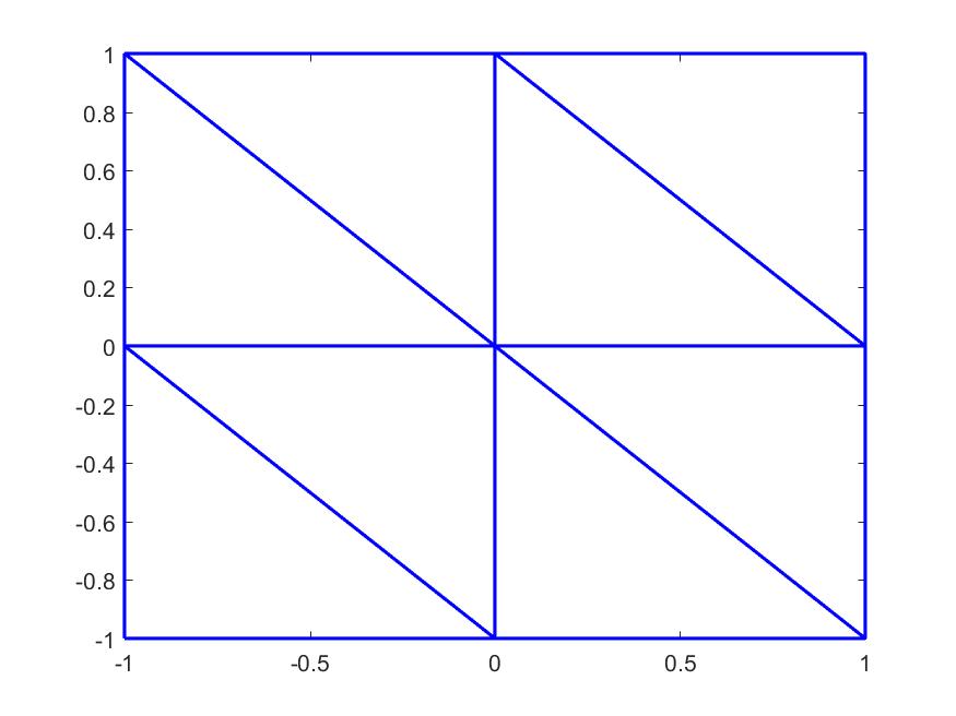
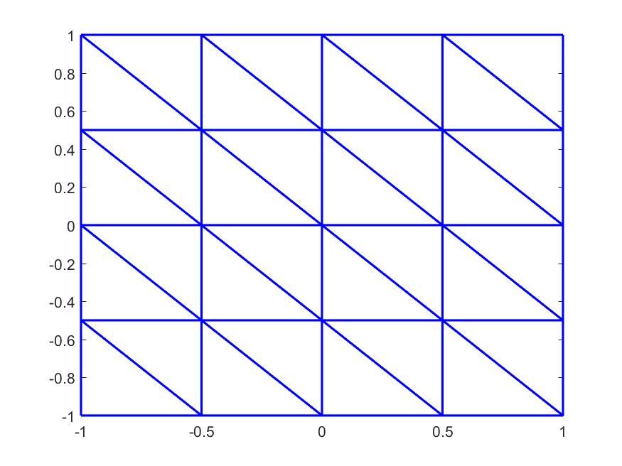
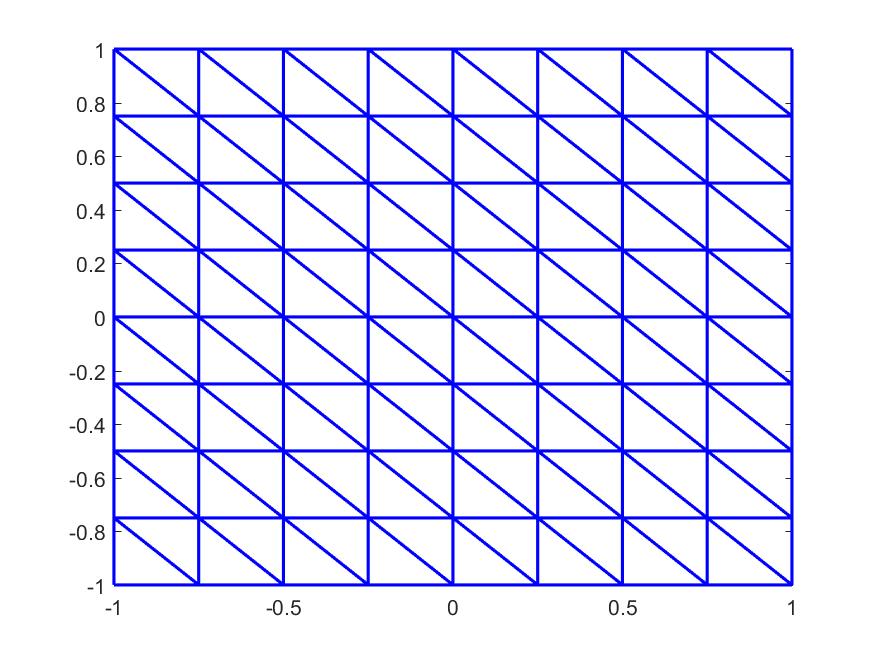
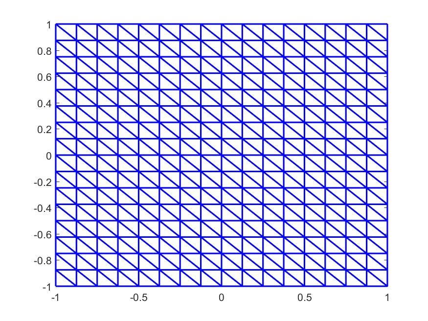
Fig. 1: Triangulations $\triangle_{\ell},\ell=0,1,2,3$

We can see that the convergences of our spline method in Tables 9 are better than those in Table 8.5 in [23] and the gradient approximations are better than the corresponding gradients in Table 8.6 in [23]. However, our $L_{2}$ estimates are not able to achieve the accuracy in Table 8.6 in [23] using quadratic splines. More accurate solutions are obtained when splines of higher degrees are used. See Tables 10–13. This example was initially studied in [20]. See Fig. 2 in [20]. For $d=2$, we are able to achieve the accuracy of $6.841801e-02$ at the size $h=0.0313$ for the accuracy of $\nabla^{2}(u-S_{u}).$

Instead of showing the convergence rates of $|u-u_{h}|_{H^{2}(\Omega)}$ in a semi-log graph for various $d=2,3,4,5$ in [20], we present more detailed numerical convergence in root mean squared error (RMSE) for $u-u_{h},\nabla(u-u_{h}),$ as well as $|D_{x}^{2}(u-u_{h})|+|D_{x}D_{y}(u-u_{h})|+|D^{2}_{y}(u-u_{h})$ based on $333\times 333$ equally-spaced points over $\Omega=[-1,1]\times[-1,1]$.

$|\triangle|$	$u-S_{u}$	rate	$\nabla(u-S_{u})$	rate	$\nabla^{2}(u-S_{u})$	rate
0.7071	4.996969e-02	0.00	1.180311e-01	0.00	4.068785e-01	0.00
0.3536	4.359043e-02	0.20	1.014477e-01	0.22	3.228522e-01	0.33
0.1768	2.742714e-02	0.67	6.679062e-02	0.60	2.187010e-01	0.56
0.0884	1.192668e-02	1.20	3.080064e-02	1.12	1.122648e-01	0.96

Table 9: The RMSE of spline solutions using the pair $X_{h}=S^{-1}_{2}(\triangle_{\ell}),M_{h}=S^{-1}_{0}(\triangle_{\ell})$ of spline spaces for $\ell=0,1,2,3,4$ of PDE (6.2) based on uniform triangulations in Figure 1

$|\triangle|$	$u-S_{u}$	rate	$\nabla(u-S_{u})$	rate	$\nabla^{2}(u-S_{u})$	rate
0.7071	2.251481e-02	0.00	5.717663e-02	0.00	2.307563e-01	0.00
0.3536	3.531272e-03	2.67	1.098214e-02	2.38	5.867175e-02	1.98
0.1768	4.842512e-04	2.87	1.699877e-03	2.69	1.261068e-02	2.22
0.0884	8.728429e-05	2.47	3.148312e-04	2.43	2.826181e-03	2.16

Table 10: The RMSE of spline solutions using the pair $X_{h}=S^{-1}_{3}(\triangle_{\ell}),M_{h}=S^{-1}_{1}(\triangle_{\ell})$ of spline spaces for $\ell=0,1,2,3,4$ of PDE (6.2) based on uniform triangulations in Figure 1

$|\triangle|$	$u-S_{u}$	rate	$\nabla(u-S_{u})$	rate	$\nabla^{2}(u-S_{u})$	rate
0.7071	1.297545e-03	0.00	3.501439e-03	0.00	2.743879e-02	0.00
0.3536	7.214648e-05	4.17	2.100133e-04	4.06	3.458414e-03	2.99
0.1768	4.215572e-06	4.10	1.213607e-05	4.11	3.941213e-04	3.13
0.0884	2.399293e-07	4.14	7.071917e-07	4.10	4.553490e-05	3.11

Table 11: The RMSE of spline solutions using the pair $X_{h}=S^{-1}_{4}(\triangle_{\ell}),M_{h}=S^{-1}_{2}(\triangle_{\ell})$ of spline spaces for $\ell=0,1,2,3,4$ of PDE (6.2) based on uniform triangulations in Figure 1

$|\triangle|$	$u-S_{u}$	rate	$\nabla(u-S_{u})$	rate	$\nabla^{2}(u-S_{u})$	rate
0.7071	4.204985e-05	0.00	2.212172e-04	0.00	2.973071e-03	0.00
0.3536	2.322110e-06	4.18	8.539613e-06	4.70	1.945146e-04	3.92
0.1768	1.418182e-07	4.03	3.877490e-07	4.46	1.172927e-05	4.04
0.0884	8.751103e-09	4.02	2.151534e-08	4.17	7.033378e-07	4.06

Table 12: The RMSE of spline solutions using the pair $X_{h}=S^{-1}_{5}(\triangle_{\ell}),M_{h}=S^{-1}_{3}(\triangle_{\ell})$ of spline spaces for $\ell=0,1,2,3,4$ of PDE (6.2) based on uniform triangulations in Figure 1

$|\triangle|$	$u-S_{u}$	rate	$\nabla(u-S_{u})$	rate	$\nabla^{2}(u-S_{u})$	rate
0.7071	3.172567e-06	0.00	1.554581e-05	0.00	2.401833e-04	0.00
0.3536	4.869340e-08	6.03	2.888992e-07	5.75	8.574254e-06	4.79
0.1768	7.439441e-10	6.03	4.886180e-09	5.89	2.752530e-07	4.95
0.0884	7.196367e-12	6.69	7.790660e-11	5.97	8.597503e-09	5.00

Table 13: The RMSE of spline solutions using the pair $X_{h}=S^{-1}_{6}(\triangle_{\ell}),M_{h}=S^{-1}_{4}(\triangle_{\ell})$ of spline spaces for $\ell=0,1,2,3,4$ of PDE (6.2) based on uniform triangulations in Figure 1

$|\triangle|$	$u-S_{u}$	rate	$\nabla(u-S_{u})$	rate	$\nabla^{2}(u-S_{u})$	rate
0.7071	2.593663e-07	0.00	7.442269e-07	0.00	1.217246e-05	0.00
0.3536	4.280178e-09	5.92	8.943363e-09	6.38	2.025671e-07	5.90
0.1768	7.233371e-11	5.89	1.274428e-10	6.13	3.166771e-09	5.99

Table 14: The RMSE of spline solutions using the pair $X_{h}=S^{-1}_{7}(\triangle_{\ell}),M_{h}=S^{-1}_{5}(\triangle_{\ell})$ of spline spaces for $\ell=1,2,3$ of PDE (6.2) based on uniform triangulations in Figure 1

$|\triangle|$	$u-S_{u}$	rate	$\nabla(u-S_{u})$	rate	$\nabla^{2}(u-S_{u})$	rate
0.7071	8.731770e-09	0.00	3.136707e-08	0.00	6.080104e-07	0.00
0.3536	5.745609e-11	7.25	1.807841e-10	7.44	5.399368e-09	6.81
0.1768	1.079912e-11	2.41	2.701168e-11	2.74	8.501408e-10	2.69

Table 15: The RMSE of spline solutions using the pair $X_{h}=S^{-1}_{8}(\triangle_{\ell}),M_{h}=S^{-1}_{6}(\triangle_{\ell})$ of spline spaces for $\ell=1,2,3$ of PDE (6.2) based on uniform triangulations in Figure 1

In Table 15, the expected accurate solutions for degree $8$ at the triangulation with size $0.1768$ were not able to achieve due to the limitation of our iterative algorithm CImin.m. Numerical convergence in Tables 9 –15 provide more evidence that the convergence $|u-u_{h}|_{H^{2}(\Omega)}$ is of order $d-1$ for $d=2,3,\cdots,8$. In addition, the convergence rate for $\|u-u_{h}\|_{L^{2}(\Omega)}$ can be better than $d-1$ for various $d$.

6.3 Numerical Results of PDE in (1.1) with nonzero $c$

In this subsection, we present some numerical results from our bivariate spline method for numerical solution of the PDE in (1.1) with nonzero $c$. We use three examples to demonstrate that our method is effective and efficient no matter the PDE coefficients are smooth or not smooth and the solutions are smooth or not so smooth.

Example 6.3.

We begin with a 2nd order elliptic equation with smooth coefficients and smooth solution $u=\sin(\pi x)\sin(\pi y)$ which satisfies the following partial differential equation:

(6.3) $$3\frac{\partial^{2}}{\partial x^{2}}u+2\frac{\partial^{2}}{\partial x\partial y}u+2\frac{\partial^{2}}{\partial y^{2}}u-(1+x^{2}+y^{2})u=f(x,y),\quad(x,y)\in\Omega\subset\mathbb{R}^{2},$$

where $\Omega$ is a standard square domain $[-1,1]^{2}$ which is split into 4 equal sub-squares and each sub-square is split into 2 triangles to form an initial triangulation $\triangle_{0}$. Let $\triangle_{\ell}$ be the $\ell$th uniform refinement of $\triangle_{0}$.

$|\triangle|$	$u-S_{u}$	rate	$\nabla(u-S_{u})$	rate	$\nabla^{2}(u-S_{u})$	rate
0.7071	7.148997e-04	0.00	5.688698e-03	0.00	7.513832e-02	0.00
0.3536	2.651667e-05	4.75	1.861396e-04	4.93	4.596716e-03	3.99
0.1768	1.257317e-06	4.40	6.093065e-06	4.93	2.814578e-04	4.03
0.0884	7.088746e-08	4.15	2.550376e-07	4.58	1.753997e-05	4.00

Table 16: The RMSE of spline solutions using the pair $X_{h}=S^{-1}_{5}(\triangle_{\ell}),M_{h}=S^{-1}_{5}(\triangle_{\ell})$ of spline spaces for $\ell=1,2,3,4$ of PDE (6.3)

Example 6.4.

In this example, we use our spline method to solve the following PDE with non-differentiable coefficients, but smooth solution.

(6.4) $$a(x,y)\frac{\partial^{2}}{\partial x^{2}}u+b(x,y)\frac{\partial^{2}}{\partial x\partial y}u+c(x,y)\frac{\partial^{2}}{\partial y^{2}}u-(1+x^{2}+y^{2})u=f(x,y),\quad(x,y)\in\Omega\subset\mathbb{R}^{2}$$

where $a(x,y)=1+|x|,b(x,y)=(xy)^{1/3},c(x,y)=1+|y|$ and $\Omega$ is a standard domain $[-1,1]^{2}$. We use $u=\sin(\pi x)\sin(\pi y)$ as the exact solution. The same triangulations $\triangle_{\ell}$ as in Example 6.3 will be used.

$|\triangle|$	$u-S_{u}$	rate	$\nabla(u-S_{u})$	rate	$\nabla^{2}(u-S_{u})$	rate
0.7071	5.906274e-04	0.00	5.894580e-03	0.00	9.080845e-02	0.00
0.3536	1.155544e-05	5.68	1.785330e-04	5.05	5.673534e-03	3.97
0.1768	3.265019e-07	5.15	4.834318e-06	5.21	3.150799e-04	4.15
0.0884	1.568269e-08	4.38	1.463029e-07	5.05	1.866297e-05	4.07

Table 17: The RMSE of spline solutions using the pair $X_{h}=S^{-1}_{5}(\triangle_{\ell}),M_{h}=S^{-1}_{5}(\triangle_{\ell})$ of spline spaces for $\ell=1,2,3,4$ of PDE (6.4)

Example 6.5.

In this example, we show the performance of our spline solutions for a PDE with nondifferentiable coefficients and nonsmooth exact solution $u=xy(e^{1-|x|}-1)(e^{1-|y|}-1)$ which satisfies

(6.5) $$2\frac{\partial^{2}}{\partial x^{2}}u+2\hbox{sign}(x)\hbox{sign}(y)\frac{\partial^{2}}{\partial x\partial y}u+2\frac{\partial^{2}}{\partial y^{2}}u-(1+x^{2}+y^{2})u=f(x,y),\quad(x,y)\in\Omega\subset\mathbb{R}^{2}$$

where $u=0$ on the boundary of $\Omega=[-1,1]\times[-1,1]$ as in [20]. Note that the solution is in $H^{2}(\Omega)$, but not continuously twice differentiable. The same triangulations $\triangle_{\ell}$ as in Example 6.3 will be used and $S^{1}_{5}(\triangle_{\ell})$ will be used to solve the PDE in (6.5). The RMSE for spline approximation to the exact solution is shown in Table 18.

$|\triangle|$	$u-S_{u}$	rate	$\nabla(u-S_{u})$	rate	$\nabla^{2}(u-S_{u})$	rate
0.7071	2.914706e-02	0.00	2.813852e-01	0.00	4.122223e+00	0.00
0.3536	8.047145e-04	5.18	1.287751e-02	4.46	3.279903e-01	3.63
0.1768	2.963898e-05	4.76	3.942771e-04	5.02	1.893540e-02	4.06
0.0884	1.403774e-06	4.40	1.307268e-05	4.91	1.139668e-03	4.05

Table 18: The RMSE of spline solutions using the pair $X_{h}=S^{-1}_{5}(\triangle_{\ell}),M_{h}=S^{-1}_{5}(\triangle_{\ell})$ of spline spaces for $\ell=1,2,3,4$ of PDE (6.5)

$|\triangle|$	$u-S_{u}$	rate	$\nabla(u-S_{u})$	rate	$\nabla^{2}(u-S_{u})$	rate
0.7071	3.494139e-06	0.00	1.538901e-05	0.00	2.054258e-04	0.00
0.3536	7.686885e-08	5.51	3.531160e-07	5.45	7.914461e-06	4.70
0.1768	1.370000e-09	5.81	6.565436e-09	5.75	2.731226e-07	4.86
0.0884	1.598556e-11	6.42	7.840289e-11	6.39	8.199009e-09	5.06

Table 19: The RMSE of spline solutions using the pair $X_{h}=S^{-1}_{6}(\triangle_{\ell}),M_{h}=S^{-1}_{6}(\triangle_{\ell})$ of spline spaces for $\ell=1,2,3,4$ of PDE (6.5)

$|\triangle|$	$u-S_{u}$	rate	$\nabla(u-S_{u})$	rate	$\nabla^{2}(u-S_{u})$	rate
0.7071	6.099647e-08	0.00	4.914744e-07	0.00	1.004845e-05	0.00
0.3536	9.745659e-10	5.97	4.297639e-09	6.84	1.659379e-07	5.92
0.1768	9.091448e-12	6.74	5.183151e-11	6.37	3.038997e-09	5.78

Table 20: The RMSE of spline solutions using the pair $X_{h}=S^{-1}_{7}(\triangle_{\ell}),M_{h}=S^{-1}_{7}(\triangle_{\ell})$ of spline spaces for $\ell=1,2,3,4$ of PDE (6.5)

In addition, we have also experimented the convergence of our bivariate spline method over nonconvex domains. The bivariate spline method works very well. Due to the space limit, we omit these numerical results.

References

- [1] G. Awanou, Robustness of a spline element method with constraints. J. Sci. Comput., 36(3):421–432, 2008.
- [2] G. Awanou, Spline element method for Monge-Amp re equations. BIT 55 (2015), no. 3, 625 -646.
- [3] G. Awanou, M. -J. Lai, and P. Wenston. The multivariate spline method for scattered data fitting and numerical solution of partial differential equations. In Wavelets and splines: Athens 2005, pages 24–74. Nashboro Press, Brentwood, TN, 2006.
- [4] I. Babuska, The finite element method with Lagrange multipliers, Numer. Math., 20 (1973), pp. 179–192.
- [5] S. C. Brenner and L. R. Scott, The mathematical theory of finite element methods, Springer Verlag, New York, 1994.
- [6] F. Brezzi, On the existence, uniqueness, and approximation of saddle point problems arising from Lagrange multipliers, RAIRO, 8 (1974), pp. 129–151.
- [7] P. G. Ciarlet, The Finite Element Method for Elliptic Problems, North–Holland, 1978.
- [8] M. Dauge, Elliptic boundary value problems on corner domains, Lecture Notes in Math., 1341, Springer Verlag, Berlin, 1988.
- [9] L. Evens, Partial Differential Equations, American Math. Society, Providence, 1998.
- [10] G. Farin, Triangular bernstein-bézier patches. Computer Aided Geometric Design, 3(2):83–127, 1986.
- [11] P. Grisvard, Elliptic Problems in Nonsmooth Domains, Pitman, Boston, 1985.
- [12] J. Gutierrez, M. -J. Lai, and Slavov, G., Bivariate Spline Solution of Time Dependent Nonlinear PDE for a Population Density over Irregular Domains, Mathematical Biosciences, vol. 270 (2015) pp. 263–277.
- [13] X. Hu, Han, D. and Lai, M. -J., Bivariate Splines of Various Degrees for Numerical Solution of PDE, SIAM Journal of Scientific Computing, vol. 29 (2007) pp. 1338–1354.
- [14] B.-N. Jiang, The Least-Squares Finite Element Method, Springer, 1998.
- [15] O. D. Kellogg, On bounded polynomials in several variables, Math. Z. 27(1928), 55–64.
- [16] M. -J. Lai and L. L. Schumaker, Spline Functions over Triangulations, Cambridge University Press, 2007.
- [17] M. -J. Lai and Wenston, P., Bivariate Splines for Fluid Flows, Computers and Fluids, vol. 33 (2004) pp. 1047–1073.
- [18] A. Maugeri, D. K. Palagachev, and L. G. Softova, Elliptic and parabolic equations with discontinuous coefficients, vol. 109 of Mathematical Research, Wiley-VCH Verlag, Berlin, 2000.
- [19] L. L. Schumaker, Spline Functions: Computational Methods, SIAM Publication, 2015.
- [20] I. Smears and E. Süli, Discontinuous Galerking finite element approximation of nondivergence form elliptic equations with Cordés coefficients, SIAM J Numer. Anal., Vol. 51, No. 4, 2013, pp. 2088–2106.
- [21] E. Süli, A brief excursion into the mathematical theory of mixed finite element methods, Lecture Notes, University of Oxford, 2013.
- [22] C. Wang and J. Wang, An efficient numerical scheme for the biharmonic equation by weak Galerkin finite element methods on polygonal or polyhedral meshes. Comput. Math. Appl. 68 (2014), no. 12, part B, 2314–2330.
- [23] C. Wang and J. Wang, A primal-dual weak Galerkin finite element method for second order elliptic equations in non-divergence form, in revision, submitted to Math. Comp. arXiv:1510.03488v1.
- [24] J. Wang and X. Ye, A weak Galerkin mixed finite element method for second-order elliptic problems, Math. Comp., 83 (2014), 2101–2126.
- [25] D. R. Wilhelmsen, A Markov inequality in several dimension, Journal Approximation Theory, 11(1974), 216–220.