Higgs-Higgs Interaction.
The One-Loop Amplitude in the Standard Model

Abstract

The amplitude of Higgs-Higgs interaction is calculated in the Standard Model in the framework of the Sirlin’s renormalization scheme in the unitary gauge. The one-loop corrections for $\lambda$, the constant of $4\chi$ interaction are compared with the previous results of L. Durand et al. obtained on using the technique of the equivalence theorem, and in the different gauges.

1 Introduction.

The Higgs sector of the electroweak theory attracts much attention because of its connection with the cornerstones of the theory. The search for Higgs scalars is included in most of the experimental programs of the newcoming and acting accelerators [2]. The Higgs particles are suggested to be found in the decays of different particles ($Z^{0}$ bosons, heavy quarkoniums etc.) as well as in photon-photon interactions and gluon-gluon fusion. In connection with that, let us mention non-so-long-ago attempts to explain anomalous events seen at SpS as the manifestation of the bound state of two Higgs bosons, i. e. of Higgsonium [3]-[5] or that of the bound state of vector boson [6] in accordance with the Veltman paper, Ref. [7]. Nowadays, even after clarifying the experimental situation with these anomalous events, the interest in Higgsonium has still the rights for existence at least from the viewpoint of preparedness to new unexpected news from the experiment. The previous investigations of the problem of existence of two-Higgs bound states were based on the Born approximation of their interaction amplitude [3]-[5]. In the present paper we present the results of our calculation of the amplitude of Higgs-Higgs interaction up to the fourth order in the framework of the Standard Model (SM) of Weinberg, Salam and Glashow with one Higgs doublet. This problem is also of present interest since there is some relations with the idea that gauge vector bosons could originate from a strong interacting scalar sector of the electroweak theory [8]. The amplitude obtained in this paper could also be useful for the consideration of the problem of the unitarity limit (e. g., [9]). Moreover, information on the behaviour of the Higgs coupling constants at mass scale $M$ would be also of interest.

These are the reasons why we start a more complete study of the problem of Higgs-Higgs interaction. To reduce the volume of the article we shall use the standard notation used in [10], dimensional regularization and the renormalization scheme on the mass shell, which is analogous to that suggested in [10, 11]. We also choose the unitary gauge ($\xi\rightarrow\infty$, to avoid ghosts) and the parameters recommended by the Trieste conference [12], namely ($e_{0},M_{W_{0}},M_{Z_{0}},M_{H_{0}},m_{f_{0}}$).

The Higgs sector of the Lagrangian of the SM with one Higgs field has the following form, e. g. [13]:

$${\cal L}=-{1\over 2}(\partial_{\mu}\chi)^{2}-{1\over 2}M_{\chi}^{2}\chi^{2}-\frac{e}{2M_{W}(1-R)^{1/2}}\sum_{f}m_{f}\bar{f}f\chi-$$ (1.1)

$$- \frac{eM_{W}}{(1-R)^{1/2}}W_{\mu}^{+}W_{\mu}^{-}\chi-\frac{eM_{Z}}{2R^{1/2}(1-R)^{1/2}}Z_{\mu}^{2}\chi-\frac{e^{2}}{4(1-R)}W_{\mu}^{+}W_{\mu}^{-}\chi^{2}-$$

$$- \frac{e^{2}}{8R(1-R)}Z_{\mu}^{2}\chi^{2}-\frac{eM_{\chi}^{2}}{4M_{W}(1-R)^{1/2}}\chi^{3}-\frac{e^{2}M_{\chi}^{2}}{32M_{W}^{2}(1-R)}\chi^{4}\,,$$

where $e$ is the electron charge, $M_{\chi}$ is the Higgs mass, $M_{W}$ and $M_{Z}$ are the masses of the vector bosons, $m_{f}$ are the fermion masses, $R=M_{W}^{2}/M_{Z}^{2}$.

The paper is organized as follows. In Section 2 we present the expressions for the self-energy and vertex parts (see also calculations in details in [14]). The results of the calculation of the total Higgs-Higgs amplitude will be presented in Section 3. The Appendix contains the definitions of some integrals met in calculations. Their connections with the integrals calculated in [15, 16] is given.

Table I. Coupling constants in the case of the Standard Model.

$f^{W}$	$-{1\over{2\sqrt{2}}}g$	$f^{WWZA}$	$ig^{2}\sqrt{R(1-R)}$
$f^{Z}$	$-{1\over 4}\frac{gM_{Z}}{M_{W}}$	$f^{W\chi}$	$-igM_{W}$
$f^{A}$	$eQ_{i}$	$f^{Z\chi}$	$-i\frac{gM_{Z}^{2}}{M_{W}}$
$f^{WWZ}$	$-\frac{gM_{W}}{M_{Z}}$	$f^{2W2\chi}$	$-i\frac{g^{2}}{2}$
$f^{WWA}$	$e$	$f^{2Z2\chi}$	$-i\frac{g^{2}M_{Z}^{2}}{2M_{W}^{2}}$
$f^{2W2Z}$	$-i\frac{g^{2}M_{W}^{2}}{M_{Z}^{2}}$	$f^{\chi}$	$-i\frac{gm_{i}}{2M_{W}}$
$f^{4W}$	$ig^{2}$	$f^{3\chi}$	$-i\frac{3gM_{\chi}^{2}}{2M_{W}}$
$f^{2W2A}$	$-ie^{2}$	$f^{4\chi}$	$-i\frac{3g^{2}M_{\chi}^{2}}{4M_{W}^{2}}$

The Kobayashi-Maskawa $K_{ij}$ matrix, $g=e/\sin\theta_{W}$ are used in the full Lagrangian of the SM, $2P=-\frac{1}{\epsilon}+\gamma+ln(M_{W}^{2}/4\pi\mu^{2})$ are used in the dimensional regularization, $\gamma$ is the Euler constant.

2 Self-energy, vertex and box diagrams for the scalar boson.

2.1 Self-energy diagrams.

Here they are:

Figure 1:

$$\Pi=\frac{if^{4\chi}}{16\pi^{2}}M_{\chi}^{2}\left[2P-1+\log\,{M_{\chi}^{2}\over M_{W}^{2}}\right].$$ (2.2)

Figure 2:

$$\Pi=\frac{if^{2V2\chi}}{16\pi^{2}}M_{V}^{2}\left[6P-1+3\log{M_{V}^{2}\over M_{W}^{2}}\right].$$ (2.3)

Figure 3:

$$\Pi(q^{2})=\frac{if_{1}^{3\chi}f_{2}^{3\chi}}{16\pi^{2}}\left[-2P-I_{0}(q^{2},M_{\chi}^{2},M_{\chi\prime}^{2})\right].$$ (2.4)

Figure 4:

$$\Pi(q^{2})=\frac{if_{1}^{\chi}f_{2}^{\chi}}{4\pi^{2}}\left\{\left[(1-b_{1}b_{2})\left(q^{2}+2m_{1}^{2}+2m_{2}^{2}\right)+(1+b_{1}b_{2})2m_{1}m_{2}\right]P+\right.$$

$$+ \left.\left[{1\over 2}(1-b_{1}b_{2})\left(q^{2}+m_{1}^{2}+m_{2}^{2}\right)+(1+b_{1}b_{2})m_{1}m_{2}\right]I_{0}(q^{2},m_{1}^{2},m_{2}^{2})+\right.$$

$$+ \left.{1\over 2}(1-b_{1}b_{2})\left(m_{1}^{2}\log\,{m_{1}^{2}\over M_{W}^{2}}+m_{2}^{2}\log\,{m_{2}^{2}\over M_{W}^{2}}+{q^{2}\over 2}\right)+{1\over 2}(1+b_{1}b_{2})m_{1}m_{2}\right\}.$$

Figure 5:

$$\Pi(q^{2})=\frac{if_{1}^{V\chi}f_{2}^{V\chi}}{16\pi^{2}}\left\{\left[-{q^{4}\over 2M_{V}^{4}}-3{q^{2}\over M_{V}^{2}}-6\right]P-\right.$$

$$- \left.\left({q^{4}\over 4M_{V}^{4}}+{q^{2}\over M_{V}^{2}}+3\right)I_{0}(q^{2},M_{V}^{2},M_{V}^{2})-{q^{2}\over 2M_{V}^{2}}\log\,{M_{V}^{2}\over M_{W}^{2}}+{q^{2}\over 2M_{V}^{2}}-2\right\}.$$

In the framework of the SM with one Higgs doublet only we obtain

$$\Pi^{\chi}(q^{2})=\frac{ig^{2}}{16\pi^{2}}M_{\chi}^{2}\left\{\left[-{3\over 4}{q^{4}\over M_{W}^{2}M_{\chi}^{2}}-3{q^{2}\over M_{\chi}^{2}}-{3\over 2R}{q^{2}\over M_{\chi}^{2}}+{q^{2}\over M_{W}^{2}M_{\chi}^{2}}Tr\,m_{i}^{2}-\right.\right.$$

$$- \left.\left.3r_{W}-9r_{W}^{-1}-{9\over 2R}r_{Z}^{-1}+{6\over M_{W}^{2}M_{\chi}^{2}}Tr\,m_{i}^{4}\right]P+tadpoles+{3q^{4}\over 4M_{W}^{2}M_{\chi}^{2}}+\right.$$

$$+ \left.\left({5\over 2}+{5\over 4R}\right){q^{2}\over M_{\chi}^{2}}+{21\over 8}r_{W}+{9\over 2}r_{W}^{-1}+{9\over 4R}r_{Z}^{-1}-{3\over 2}r_{W}\log\,r_{W}+\left({q^{4}\over 8M_{W}^{4}}+\right.\right.$$

$$+ \left.\left.{3\over 4R}{q^{2}\over M_{W}^{2}}+{9\over 4R^{2}}\right)r_{W}^{-1}\log\,R-{3q^{2}\over 4M_{W}^{2}M_{\chi}^{2}}Tr\,m_{i}^{2}+\right.$$

$$+ \left.{q^{2}\over 2M_{W}^{2}M_{\chi}^{2}}Tr\,m_{i}^{2}\log\,{m_{i}^{2}\over M_{W}^{2}}-{7\over 2M_{W}^{2}M_{\chi}^{2}}Tr\,m_{i}^{4}+{3\over M_{W}^{2}M_{\chi}^{2}}Tr\,m_{i}^{4}\log\,{m_{i}^{2}\over M_{W}^{2}}-\right.$$

$$- \left.\left({q^{2}\over 8M_{W}^{2}}+{1\over 2}+{3M_{W}^{2}\over 2q^{2}}\right){1\over M_{\chi}^{2}}L(q^{2},M_{W}^{2},M_{W}^{2})-\right.$$

$$- \left.\left({q^{2}\over 16M_{Z}^{2}}+{1\over 4}+{3M_{Z}^{2}\over 4q^{2}}\right){1\over R}{1\over M_{\chi}^{2}}L(q^{2},M_{Z}^{2},M_{Z}^{2})-\right.$$

$$- \left.{9\over 16}r_{W}{1\over q^{2}}L(q^{2},M_{\chi}^{2},M_{\chi}^{2})-{1\over 4M_{W}^{2}M_{\chi}^{2}}Tr\,m_{i}^{2}L(q^{2},m_{i}^{2},m_{i}^{2})+\right.$$

$$+ \left.{1\over M_{W}^{2}M_{\chi}^{2}}{1\over q^{2}}Tr\,m_{i}^{4}L(q^{2},m_{i}^{2},m_{i}^{2})\right\}.$$

The corresponding counterterms are

$$\frac{\delta M_{\chi}^{2}}{M_{\chi}^{2}}=Z_{M_{\chi}}-Z_{\chi}=\frac{ig^{2}}{16\pi^{2}}\left\{\left[3+{3\over 2R}-{15\over 4}r_{W}-9r_{W}^{-1}-{9\over 2R}r_{Z}^{-1}-{1\over M_{W}^{2}}Tr\,m_{i}^{2}+\right.\right.$$

$$+ \left.\left.{6\over M_{W}^{2}M_{\chi}^{2}}Tr\,m_{i}^{4}\right]P+\frac{\Pi^{\chi}(tadpoles)}{M_{\chi}^{2}}-{5\over 2}-{5\over 4R}+{27\over 8}r_{W}+{9\over 2}r_{W}^{-1}+{9\over 4R}r_{Z}^{-1}-\right.$$

$$- \left.{3\over 2}r_{W}\log\,r_{W}+\left({1\over 8}r_{W}-{3\over 4R}+{9\over 4R}r_{Z}^{-1}\right)\log\,R+{3\over 4M_{W}^{2}}Tr\,m_{i}^{2}-\right.$$

$$- \left.{1\over 2M_{W}^{2}}Tr\,m_{i}^{2}\log\,{m_{i}^{2}\over M_{W}^{2}}-{7\over 2M_{W}^{2}M_{\chi}^{2}}Tr\,m_{i}^{4}+{3\over M_{W}^{2}M_{\chi}^{2}}Tr\,m_{i}^{4}\log\,{m_{i}^{2}\over M_{W}^{2}}+\right.$$

$$+ \left.\left({r_{W}\over 8}-{1\over 2}+{3\over 2}r_{W}^{-1}\right){1\over M_{\chi}^{2}}L(-M_{\chi}^{2},M_{W}^{2},M_{W}^{2})+\right.$$

$$+ \left.\left({r_{Z}\over 16}-{1\over 4}+{3\over 4}r_{Z}^{-1}\right){1\over R}{1\over M_{\chi}^{2}}L(-M_{\chi}^{2},M_{Z}^{2},M_{Z}^{2})+\right.$$

$$+ \left.{9\over 16M_{W}^{2}}L(-M_{\chi}^{2},M_{\chi}^{2},M_{\chi}^{2})+\right.$$

$$+ \left.{1\over 4M_{W}^{2}M_{\chi}^{2}}Tr\,m_{i}^{2}L(-M_{\chi}^{2},m_{i}^{2},m_{i}^{2})-{1\over M_{W}^{2}M_{\chi}^{4}}Tr\,m_{i}^{4}L(-M_{\chi}^{2},m_{i}^{2},m_{i}^{2})\right\}$$

and

$$Z_{\chi}-1=\frac{ig^{2}}{16\pi^{2}}\left\{\left[-3-{3\over 2R}+{3\over 2}r_{W}+{1\over M_{W}^{2}}Tr\,m_{i}^{2}\right]P+{3\over 2}+{3\over 4R}+3r_{W}^{-1}+\right.$$

$$+ \left.{3\over 2R}r_{Z}^{-1}+\left({3\over 4R}-{1\over 4}r_{W}\right)\log\,R-{1\over 4M_{W}^{2}}Tr\,m_{i}^{2}+{1\over 2M_{W}^{2}}Tr\,m_{i}^{2}\log\,{m_{i}^{2}\over M_{W}^{2}}-\right.$$

$$- \left.{2\over M_{W}^{2}M_{\chi}^{2}}Tr\,m_{i}^{4}+\left({1\over 4}-{1\over 4}r_{W}-{3\over r_{W}(r_{W}-4)}\right){1\over M_{\chi}^{2}}L(-M_{\chi}^{2},M_{W}^{2},M_{W}^{2})+\right.$$

$$+ \left.\left({1\over 8}-{1\over 8}r_{Z}-{3\over 2r_{Z}(r_{Z}-4)}\right){1\over R}{1\over M_{\chi}^{2}}L(-M_{\chi}^{2},M_{Z}^{2},M_{Z}^{2})+\right.$$

$$+ \left.{3\over 8}{1\over M_{W}^{2}}L(-M_{\chi}^{2},M_{\chi}^{2},M_{\chi}^{2})-\right.$$

$$- \left.{1\over 4M_{W}^{2}M_{\chi}^{2}}Tr\,m_{i}^{2}L(-M_{\chi}^{2},m_{i}^{2},m_{i}^{2})-{1\over 2M_{W}^{2}M_{\chi}^{4}}Tr\,m_{i}^{4}L(-M_{\chi}^{2},m_{i}^{2},m_{i}^{2})\right\}$$

Consequently,

$$\Pi^{ren}(q^{2})=\Pi^{\chi}(q^{2})-\delta M_{\chi}^{2}-(Z_{\chi}-1)(q^{2}+M_{\chi}^{2})=\frac{ig^{2}}{16\pi^{2}}M_{\chi}^{2}\times$$ (2.10)

$$\times \left\{\left[-{3\over 4}{q^{4}\over M_{W}^{2}M_{\chi}^{2}}-{3\over 4}r_{W}-{3\over 2}{q^{2}\over M_{W}^{2}}\right]P+{3q^{4}\over 4M_{W}^{2}M_{\chi}^{2}}+{q^{4}\over 8M_{W}^{2}M_{\chi}^{2}}\log\,R+\right.$$

$$+ \left.{q^{2}\over M_{\chi}^{2}}\left(1+{1\over 2R}-3r_{W}^{-1}-{3\over 2R}r_{Z}^{-1}\right)+{q^{2}\over 4M_{W}^{2}}\log\,R+{1\over 8}r_{W}\log\,R+\right.$$

$$+ \left.1+{1\over 2R}-{3\over 4}r_{W}-3r_{W}^{-1}-{3\over 2R}r_{Z}^{-1}-\left({q^{2}\over M_{\chi}^{2}}+1\right){1\over 2M_{W}^{2}}Tr\,m_{i}^{2}+\right.$$

$$+ \left.\left({q^{2}\over M_{\chi}^{2}}+1\right){2\over M_{W}^{2}M_{\chi}^{2}}Tr\,m_{i}^{4}-\left({q^{2}\over 8M_{W}^{2}}+{1\over 2}+{3M_{W}^{2}\over 2q^{2}}\right)\times\right.$$

$$\times \left.{1\over M_{\chi}^{2}}L(q^{2},M_{W}^{2},M_{W}^{2})-\left({q^{2}\over 16M_{Z}^{2}}+{1\over 4}+{3M_{Z}^{2}\over 4q^{2}}\right){1\over R}{1\over M_{\chi}^{2}}L(q^{2},M_{Z}^{2},M_{Z}^{2})-\right.$$

$$- \left.{9\over 16q^{2}}r_{W}L(q^{2},M_{\chi}^{2},M_{\chi}^{2})+{1\over 4M_{W}^{2}M_{\chi}^{2}}Tr\,m_{i}^{2}L(q^{2},m_{i}^{2},m_{i}^{2})+\right.$$

$$+ \left.{1\over M_{W}^{2}M_{\chi}^{2}}{1\over q^{2}}Tr\,m_{i}^{4}L(q^{2},m_{i}^{2},m_{i}^{2})+\left(-{q^{2}\over 4M_{\chi}^{2}}+{q^{2}\over 4M_{W}^{2}}-{3q^{2}\over M_{\chi}^{2}r_{W}(r_{W}-4)}+\right.\right.$$

$$+ \left.\left.{1\over 4}+{1\over 8}r_{W}-{3\over 2}r_{W}^{-1}+{3\over r_{W}(r_{W}-4)}\right){1\over M_{\chi}^{2}}L(-M_{\chi}^{2},M_{W}^{2},M_{W}^{2})+\right.$$

$$+ \left.\left(-{q^{2}\over 8M_{\chi}^{2}}+{q^{2}\over 8M_{Z}^{2}}+{3q^{2}\over M_{\chi}^{2}r_{Z}(r_{Z}-4)}+{1\over 8}+{1\over 16}r_{Z}-{3\over 4}r_{Z}^{-1}+\right.\right.$$

$$+ \left.\left.{3\over 2r_{Z}(r_{Z}-4)}\right){1\over R}{1\over M_{\chi}^{2}}L(-M_{\chi}^{2},M_{Z}^{2},M_{Z}^{2})-\right.$$

$$- \left.\left({3q^{2}\over 8M_{W}^{2}}+{15\over 16}r_{W}\right){1\over M_{\chi}^{2}}L(-M_{\chi}^{2},M_{\chi}^{2},M_{\chi}^{2})+\right.$$

$$+ \left.{q^{2}\over 4M_{W}^{2}M_{\chi}^{4}}Tr\,m_{i}^{2}L(-M_{\chi}^{2},m_{i}^{2},m_{i}^{2})+{1\over 2M_{W}^{2}M_{\chi}^{4}}\left(3+{q^{2}\over M_{\chi}^{2}}\right)\times\right.$$

$$\times \left.Tr\,m_{i}^{4}L(-M_{\chi}^{2},m_{i}^{2},m_{i}^{2})\right\}$$

In this Section and in what follows $r_{W}=M_{\chi}^{2}/M_{W}^{2}$, $r_{Z}=M_{\chi}^{2}/M_{Z}^{2}$, $b_{1,2}$ are constants defined by the strength of the Higgs -fermion pseudoscalar interaction. The form of the integral $I_{0}(q^{2},M_{1}^{2},M_{2}^{2})$ is given in Appendix A.

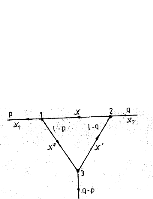
Figure 6:

2.2 Vertex diagrams.

The technique of the calculation of the diagrams shown below is very much alike to that suggested in paper [16].

$$\Gamma(p^{2},q^{2},(p-q)^{2})=\frac{if_{1}^{3\chi}f_{2}^{3\chi}f_{3}^{3\chi}}{16\pi^{2}}I_{1}(q^{2},(p-q)^{2},p^{2},M_{\chi}^{2},M_{\chi^{\prime}}^{2},M_{\chi^{\prime\prime}}^{2}).$$ (2.11)

and a similar diagram with the opposite lepton current direction give

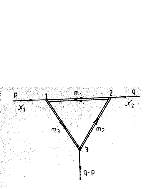
Figure 7:

$$\Gamma(p^{2},q^{2},(p-q)^{2})=\frac{if_{1}^{\chi}f_{2}^{\chi}f_{3}^{\chi}}{4\pi^{2}}\left\{\left[-2m_{1}B_{1}-2m_{2}B_{2}-2m_{3}B_{3}\right]P-\right.$$

$$- \left.\frac{m_{1}B_{1}+m_{2}B_{2}+m_{3}B_{3}}{2}-\frac{m_{1}B_{1}+m_{2}B_{2}}{2}I_{0}(q^{2},m_{1}^{2},m_{2}^{2})-\right.$$

$$- \left.\frac{m_{1}B_{1}+m_{3}B_{3}}{2}I_{0}(p^{2},m_{1}^{2},m_{3}^{2})-\frac{m_{2}B_{2}+m_{3}B_{3}}{2}I_{0}((p-q)^{2},m_{2}^{2},m_{3}^{2})-\right.$$

$$- \left.{1\over 2}\left[\left(m_{1}(p-q)^{2}+m_{1}m_{2}^{2}+m_{1}m_{3}^{2}\right)B_{1}+\right.\right.$$

$$+ \left.\left.\left(m_{2}p^{2}+m_{2}m_{1}^{2}+m_{2}m_{3}^{2}\right)B_{2}+\left(m_{3}q^{2}+m_{3}m_{1}^{2}+m_{3}m_{2}^{2}\right)B_{3}+\right.\right.$$

$$+ \left.\left.2m_{1}m_{2}m_{3}B_{4}\right]I_{1}(q^{2},(p-q)^{2},p^{2},m_{1}^{2},m_{2}^{2},m_{3}^{2})\right\}.$$

where

$$B_{1} = 1+b_{1}b_{2}-b_{1}b_{3}-b_{2}b_{3},$$

$$B_{2} = 1-b_{1}b_{2}-b_{1}b_{3}+b_{2}b_{3},$$

$$B_{3} = 1-b_{1}b_{2}+b_{1}b_{3}-b_{2}b_{3},$$

$$B_{4} = 1+b_{1}b_{2}+b_{1}b_{3}+b_{2}b_{3}.$$ (2.12)

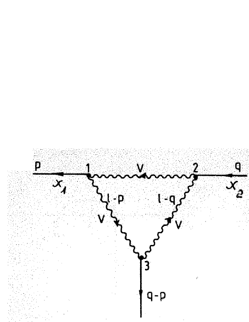
Figure 8:

and a similar diagram with the opposite loop current direction

$$\Gamma(p^{2},q^{2},(p-q)^{2})=\frac{if_{1}^{V\chi}f_{2}^{V\chi}f_{3}^{V\chi}}{16\pi^{2}}\left\{\left[-{3\over 4}\frac{p^{2}+q^{2}+(p-q)^{2}}{M_{V}^{4}}-\right.\right.$$ (2.13)

$$- \left.\left.{1\over 8}\frac{(p^{2}+q^{2}+(p-q)^{2})^{2}}{M_{V}^{6}}\right]P+\frac{p^{2}+q^{2}+(p-q)^{2}}{4M_{V}^{4}}\left(1-\log\,{M_{V}^{2}\over M_{W}^{2}}\right)-\right.$$

$$- \left.\left[{1\over 4M_{V}^{4}}\left(\frac{p^{2}+q^{2}-(p-q)^{2}}{2}+p^{2}-q^{2}\right)+\frac{p^{2}(p^{2}+q^{2}+(p-q)^{2})}{16M_{V}^{6}}\right]\times\right.$$

$$\times \left.I_{0}(p^{2},M_{V}^{2},M_{V}^{2})-\left[{1\over 4M_{V}^{4}}\left({p^{2}+q^{2}-(p-q)^{2}\over 2}+q^{2}-p^{2}\right)+\right.\right.$$

$$+ \left.\left.\frac{q^{2}(p^{2}+q^{2}+(p-q)^{2})}{16M_{V}^{6}}\right]I_{0}(q^{2},M_{V}^{2},M_{V}^{2})+\left[{1\over 4M_{V}^{4}}\left({p^{2}+q^{2}-(p-q)^{2}\over 2}-\right.\right.\right.$$

$$- \left.\left.\left.(p-q)^{2}\right)-\frac{(p-q)^{2}(p^{2}+q^{2}+(p-q)^{2})}{16M_{V}^{6}}\right]I_{0}((p-q)^{2},M_{V}^{2},M_{V}^{2})+\right.$$

$$+ \left.\left[3+\frac{p^{2}+q^{2}+(p-q)^{2}}{2M_{V}^{2}}+\right.\right.$$

$$+ \left.\left.\frac{p^{4}+q^{4}-p^{2}q^{2}+(p-q)^{4}-p^{2}(p-q)^{2}-q^{2}(p-q)^{2}}{4M_{V}^{4}}-\right.\right.$$

$$- \left.\left.\frac{p^{2}q^{2}(p-q)^{2}}{8M_{V}^{6}}\right]I_{1}(q^{2},(p-q)^{2},p^{2},M_{V}^{2},M_{V}^{2},M_{V}^{2})\right\}.$$

The form of the integral $I_{1}$ is also given in Appendix A.

The diagrams can be easily derived from the self-energy diagrams (see preceding Subsection). As a sum, we get

Figure 9:

$$\Gamma(p^{2},q^{2},(p-q)^{2})=\frac{ig^{3}}{16\pi^{2}}\frac{M_{\chi}^{2}}{M_{W}}\left\{\left[{3\over 4}\frac{p^{2}q^{2}+p^{2}(p-q)^{2}+q^{2}(p-q)^{2}}{M_{W}^{2}M_{\chi}^{2}}-{27\over 8}r_{W}-\right.\right.$$ (2.14)

$$- \left.\left.9r_{W}^{-1}-{9\over 2R}r_{Z}^{-1}+{6\over M_{W}^{2}M_{\chi}^{2}}Tr\,m_{i}^{6}\right]P+\Gamma^{3\chi}(tadpoles)-\frac{p^{2}+q^{2}+(p-q)^{2}}{4M_{\chi}^{2}}+\right.$$

$$+ \left.\frac{p^{2}+q^{2}+(p-q)^{2}}{8M_{\chi}^{2}}{1\over R}-{3\over 4}\frac{p^{2}q^{2}+p^{2}(p-q)^{2}+q^{2}(p-q)^{2}}{M_{W}^{2}M_{\chi}^{2}}-\right.$$

$$- \left.\frac{p^{2}q^{2}+p^{2}(p-q)^{2}+q^{2}(p-q)^{2}}{8M_{W}^{2}M_{\chi}^{2}}\log R+{27\over 8}r_{W}-{27\over 16}r_{W}\log r_{W}+6r_{W}^{-1}+\right.$$

$$+ \left.3{1\over R}r_{Z}^{-1}++{9\over 4}r_{Z}^{-1}{1\over R}\log R-{9\over 2M_{W}^{2}M_{\chi}^{2}}Tr\,m_{i}^{4}+\frac{3}{M_{W}^{2}M_{\chi}^{2}}Tr\ m_{i}^{4}\log{m_{i}^{2}\over M_{W}^{2}}-\right.$$

$$+ \left.\left[-{3\over 2}r_{W}^{-1}-\frac{q^{2}+(p-q)^{2}-p^{2}}{4M_{\chi}^{2}}+\frac{p^{2}(q^{2}+(p-q)^{2})}{8M_{W}^{2}M_{\chi}^{2}}\right]\times\right.$$

$$\times \left.{1\over 2p^{2}}L(p^{2},M_{W}^{2},M_{W}^{2})+\left[-{3\over 2}r_{W}^{-1}-\frac{p^{2}+(p-q)^{2}-q^{2}}{4M_{\chi}^{2}}+\frac{q^{2}(p^{2}+(p-q)^{2})}{8M_{W}^{2}M_{\chi}^{2}}\right]\times\right.$$

$$\times \left.{1\over 2q^{2}}L(q^{2},M_{W}^{2},M_{W}^{2})+\left[-{3\over 2}r_{W}^{-1}-\frac{p^{2}+q^{2}-(p-q)^{2}-p^{2}}{4M_{\chi}^{2}}+\right.\right.$$

$$+ \left.\left.\frac{(p-q)^{2}(p^{2}+q^{2})}{8M_{W}^{2}M_{\chi}^{2}}\right]{1\over(p-q)^{2}}L((p-q)^{2},M_{W}^{2},M_{W}^{2})+\right.$$

$$+ \left.\left[-{3\over 4R}r_{Z}^{-1}-\frac{q^{2}+(p-q)^{2}-p^{2}}{8M_{\chi}^{2}}{1\over R}+\frac{p^{2}(q^{2}+(p-q)^{2})}{16M_{W}^{2}M_{\chi}^{2}}\right]{1\over 2p^{2}}L(p^{2},M_{Z}^{2},M_{Z}^{2})+\right.$$

$$+ \left.\left[-{3\over 4R}r_{Z}^{-1}-\frac{p^{2}+(p-q)^{2}-q^{2}}{8M_{\chi}^{2}}{1\over R}+\frac{q^{2}(p^{2}+(p-q)^{2})}{16M_{W}^{2}M_{\chi}^{2}}\right]{1\over 2q^{2}}L(q^{2},M_{Z}^{2},M_{Z}^{2})+\right.$$

$$+ \left.\left[-{3\over 4R}r_{Z}^{-1}-\frac{p^{2}+q^{2}-(p-q)^{2}-p^{2}}{8M_{\chi}^{2}}{1\over R}+\right.\right.$$

$$+ \left.\left.\frac{(p-q)^{2}(p^{2}+q^{2})}{16M_{W}^{2}M_{\chi}^{2}}\right]{1\over 2(p-q)^{2}}L((p-q)^{2},M_{Z}^{2},M_{Z}^{2})-\right.$$

$$- \left.{9\over 16}r_{W}\left[{1\over 2p^{2}}L(p^{2},M_{\chi}^{2},M_{\chi}^{2})+{1\over 2q^{2}}L(q^{2},M_{\chi}^{2},M_{\chi}^{2})+\right.\right.$$

$$+ \left.\left.{1\over 2(p-q)^{2}}L((p-q)^{2},M_{\chi}^{2},M_{\chi}^{2})\right]+\right.$$

$$+ \left.{1\over M_{W}^{2}M_{\chi}^{2}}Tr\,m_{i}^{4}\left[{1\over 2p^{2}}L(p^{2},M_{\chi}^{2},M_{\chi}^{2})+{1\over 2q^{2}}L(q^{2},M_{\chi}^{2},M_{\chi}^{2})+\right.\right.$$

$$+ \left.\left.{1\over(p-q)^{2}}L((p-q)^{2},M_{\chi}^{2},M_{\chi}^{2})\right]-{27\over 8}r_{W}M_{\chi}^{2}I_{1}(q^{2},(p-q)^{2},p^{2},M_{\chi}^{2},M_{\chi}^{2},M_{\chi}^{2})-\right.$$

$$- \left.\left[6r_{W}^{-1}M_{W}^{2}+(p^{2}+q^{2}+(p-q)^{2})r_{W}^{-1}+\right.\right.$$

$$+ \left.\left.\frac{p^{4}+q^{4}+(p-q)^{4}-p^{2}q^{2}-p^{2}(p-q)^{2}-q^{2}(p-q)^{2}}{2M_{\chi}^{2}}-\right.\right.$$

$$- \left.\left.\frac{p^{2}q^{2}(p-q)^{2}}{4M_{W}^{2}M_{\chi}^{2}}\right]I_{1}(q^{2},(p-q)^{2},p^{2},M_{W}^{2},M_{W}^{2},M_{W}^{2})-\right.$$

$$- \left.\left[{3\over R}r_{Z}^{-1}M_{Z}^{2}+\frac{p^{2}+q^{2}+(p-q)^{2}}{2R}r_{Z}^{-1}+\right.\right.$$

$$+ \left.\left.\frac{p^{4}+q^{4}+(p-q)^{4}-p^{2}q^{2}-p^{2}(p-q)^{2}-q^{2}(p-q)^{2}}{4RM_{\chi}^{2}}-\right.\right.$$

$$- \left.\left.\frac{p^{2}q^{2}(p-q)^{2}}{8M_{W}^{2}M_{\chi}^{2}}\right]I_{1}(q^{2},(p-q)^{2},p^{2},M_{Z}^{2},M_{Z}^{2},M_{Z}^{2})+\right.$$

$$+ \left.\frac{p^{2}+q^{2}+(p-q)^{2}}{2M_{W}^{2}M_{\chi}^{2}}Trm_{i}^{4}I_{1}(q^{2},(p-q)^{2},p^{2},m_{i}^{2},m_{i}^{2},m_{i}^{2})+\right.$$

$$+ \left.{4\over M_{W}^{2}M_{\chi}^{2}}Trm_{i}^{6}I_{1}(q^{2},(p-q)^{2},p^{2},m_{i}^{2},m_{i}^{2},m_{i}^{2})\right\}.$$

The appropriate counterterm is

$$\Gamma^{c.t}=-{3gM_{\chi}^{2}\over 2M_{W}}\left[{3\over 2}(Z_{\chi}-1)+{\delta g\over g}+{\delta M_{\chi}^{2}\over M_{\chi}^{2}}-{\delta M_{W}^{2}\over 2M_{W}^{2}}\right].$$ (2.15)

As found in [10]

$${\delta g\over g}=Z_{A}^{-1/2}\left(1-\frac{\delta R}{1-R}\right)^{-1/2}-1\simeq{1\over 2}\left[\frac{\delta R}{1-R}-(Z_{A}-1)\right],$$ (2.16)

$$\frac{\delta R}{R}=\frac{Z_{M_{W}}Z_{W}^{-1}}{Z_{M_{Z}}Z_{Z}^{-1}}-1\simeq\frac{\delta M_{W}^{2}}{M_{W}^{2}}-\frac{\delta M_{Z}^{2}}{M_{Z}^{2}},$$ (2.17)

where

$$\frac{\delta M_{W}^{2}}{M_{W}^{2}}=Z_{M_{W}}-Z_{W}=\frac{ig^{2}}{16\pi^{2}}\left\{\left[{34\over 3}-{3\over 2R}-{1\over 3}N_{f}+{1\over M_{W}^{2}}Tr\,m_{i}^{2}\right]P-19+{14\over 9}+\right.$$ (2.18)

$$+ \left.{23\over 12R}+{1\over 12R^{2}}-{1\over 2}r_{W}+{1\over 12}r_{W}^{2}+(-{7\over 2}+{7\over 12R}+{1\over 24R^{2}}){1\over R}\log R+\right.$$

$$+ \left.(-{3\over 4}+{1\over 4}r_{W}-{1\over 24}r_{W}^{2})r_{W}\log r_{W}+{7\over 36}N_{f}-{1\over 12M_{W}^{2}}Trm_{i}^{2}-{1\over 6M_{W}^{4}}Trm_{i}^{4}+\right.$$

$$+ \left.\sum_{i,j}^{N_{f}/2}\left[{m_{i}^{2}m_{j}^{2}\over 3M_{W}^{4}}-({1\over 3}-\frac{m_{i}^{2}+m_{j}^{2}}{2M_{W}^{2}}\times\log{m_{i}m_{j}}{M_{W}^{2}}+\frac{(m_{i}^{2}-m_{j}^{2})^{3}}{12M_{W}^{6}}\log{m_{i}^{2}}{m_{j}^{2}}-\right.\right.$$

$$- \left.\left.({1\over 6}-\frac{m_{i}^{2}+m_{j}^{2}}{12M_{W}^{2}}-\frac{m_{i}^{2}-m_{j}^{2})^{2}}{12M_{W}^{4}}){1\over M_{W}^{2}}L(-M_{W}^{2},m_{i}^{2},m_{j}^{2})\right]K_{ij}K_{ij}^{+}+\right.$$

$$- \left.({1\over 2}-{r_{W}\over 6}+{r_{W}^{2}\over 24}){1\over M_{W}^{2}}L(-M_{W}^{2},M_{W}^{2},M_{\chi}^{2})+(-{17\over 6}-2R+{2\over 3R}+{1\over 24R^{2}})\times\right.$$

$$\times \left.{1\over M_{W}^{2}}L(-M_{W}^{2},M_{W}^{2},M_{Z}^{2})\right\},$$

and

$$\frac{\delta M_{Z}^{2}}{M_{Z}^{2}}=Z_{M_{Z}}-Z_{Z}=\frac{ig^{2}}{16\pi^{2}}\left\{\left[-{7\over 3}+14R-{11\over 6R}-\right.\right.$$ (2.19)

$$- \left.\left.{1\over 3}\left(2-{1\over 3}\right)N_{f}-{8\over 3}\frac{(1-R)^{2}}{R}Tr\,Q_{i}^{2}+{1\over M_{W}^{2}}Tr\,m_{i}^{2}\right]P+\right.$$

$$+ \left.{35\over 18}-{34\over 3}R-8R^{2}+\right.$$

$$- \left.{35\over 18R}-{1\over 2}r_{W}+{1\over 12}r_{W}r_{Z}+{5\over 6R}\log R+\left(-{3\over 4}+{1\over 4}r_{Z}-{1\over 24}r_{Z}^{2}\right)r_{W}\log r_{Z}+\right.$$

$$+ \left.\left({7\over 36}N_{f}-{14\over 9}Tr\,Q_{i}^{2}\right)\left(2-{1\over R}\right)+{14\over 9}RTr\,Q_{i}^{2}+\right.$$

$$+ \left.{1\over M_{W}^{2}}Tr\,\left[\left(-{1\over 12}-{8\over 3}|Q_{i}|+{16\over 3}Q_{i}^{2}\right)m_{i}^{2}+\left({8\over 3}|Q_{i}|-{32\over 3}Q_{i}^{2}\right)Rm_{i}^{2}+\right.\right.$$

$$+ \left.\left.{16\over 3}Q_{i}^{2}R^{2}m_{i}^{2}\right]+{1\over M_{W}^{2}}Tr\,\left[{1\over 2}m_{i}^{2}-{1\over 3}M_{Z}^{2}\left({1\over 2}-2|Q_{i}|+4Q_{i}^{2}\right)-\right.\right.$$

$$- \left.\left.{1\over 3}M_{W}^{2}\left(2|Q_{i}|-8Q_{i}^{2}\right)-{4M_{W}^{2}\over 3M_{Z}^{2}}Q_{i}^{2}\right]\log{m_{i}^{2}\over M_{W}^{2}}+\right.$$

$$+ \left.\left({1\over 24}+{2\over 3}R-{17\over 6}R^{2}-2R^{3}\right){1\over M_{W}^{2}}L(-M_{Z}^{2},M_{W}^{2},M_{W}^{2})+\right.$$

$$+ \left.\left({1\over 2}-{1\over 6}r_{Z}+{1\over 24}r_{Z}^{2}\right){1\over M_{W}^{2}}L(-M_{Z}^{2},M_{Z}^{2},M_{\chi}^{2})+\right.$$

$$+ \left.Tr\,\left[\left({1\over 12}-{1\over 3}|Q_{i}|+{2\over 3}Q_{i}^{2}\right)+\left({1\over 3}|Q_{i}|-{4\over 3}Q_{i}^{2}\right)R+{2\over 3}Q_{i}^{2}R^{2}-\right.\right.$$

$$- \left.\left.\left({1\over 12}+{2\over 3}|Q_{i}|-{4\over 3}Q_{i}^{2}\right){m_{i}^{2}\over M_{Z}^{2}}+\left({2\over 3}|Q_{i}|-{8\over 3}Q_{i}^{2}\right)R{m_{i}^{2}\over M_{Z}^{2}}+\right.\right.$$

$$+ \left.\left.{4\over 3}Q_{i}^{2}R^{2}{m_{i}^{2}\over M_{Z}^{2}}\right]{1\over M_{W}^{2}}L(-M_{Z}^{2},m_{i}^{2},m_{i}^{2})\right\}$$

Finally,

$$Z_{A}-1=\frac{ie^{2}}{16\pi^{2}}\left\{\left[-14+{8\over 3}Tr\,Q_{i}^{2}\right]P+{2\over 3}\left(1+Tr\,Q_{i}^{2}\right)+{4\over 3}Tr\,Q_{i}^{2}\log\,{m_{i}^{2}\over m_{W}^{2}}\right\}.$$ (2.20)

Thus,

$$\frac{\delta g}{g}=\frac{ig^{2}}{16\pi^{2}}\left\{\left[{43\over 6}-{1\over 6}N_{f}\right]P-{1\over 3}(1-R)\left(1+Tr\,Q_{i}^{2}+\right.\right.$$ (2.21)

$$+ \left.\left.2Tr\,Q_{i}^{2}\log\,{m_{i}^{2}\over M_{W}^{2}}\right)+{1\over 2}\frac{R}{1-R}\left[W(-1)-Z(-1)\right]\right\},$$

where $W(-1)$ and $Z(-1)$ are the finite parts of the counterterms $\delta M_{W}^{2}/M_{W}^{2}$ and $\delta M_{Z}^{2}/M_{Z}^{2}$, respectively. Then,

$$\Gamma^{c.t.}(p^{2},q^{2},(p-q)^{2})=-\frac{ig^{3}}{16\pi^{2}}\frac{3M_{\chi}^{2}}{2M_{W}}\left\{\left[-{3\over 2}r_{W}-9r_{W}^{-1}-\right.\right.$$

$$- \left.\left.{9\over 2R}r_{Z}^{-1}+{6\over M_{W}^{2}M_{\chi}^{2}}Tr\,m_{i}^{4}\right]P+\right.$$

$$+ \left.{1\over 2}\left({R\over 1-R}-1\right)W(-1)-{1\over 2}{R\over 1-R}Z(-1)+\right.$$

$$+ \left.\chi(-1)+{3\over 2}\chi^{F}(-1)-2\Gamma^{3\chi}(tadpoles)-\right.$$

$$- \left.{1\over 3}(1-R)\left(1+Tr\,Q_{i}^{2}+2Tr\,Q_{i}^{2}\log\,{m_{i}^{2}\over M_{W}^{2}}\right)\right\}=$$

$$= -{ig^{3}\over 16\pi^{2}}{3M_{\chi}^{2}\over 2M_{W}}\left\{\left[-{3\over 2}r_{W}-9r_{W}^{-1}-{9\over 2R}r_{Z}^{-1}+{6\over M_{W}^{2}M_{\chi}^{2}}Tr\,m_{i}^{4}\right]P+\right.$$

$$+ \left.{49\over 6}-{28\over 3}R-4R^{2}-{25\over 24R}-{1\over 24R^{2}}-\right.$$

$$- \left.\left({10\over 9}-{10\over 9}R\right)Tr\,Q_{i}^{2}+{29\over 8}r_{W}-{1\over 4}r_{W}^{2}+{1\over 4}r_{W}r_{Z}+9r_{W}^{-1}+{9\over 2R}r_{Z}^{-1}+\right.$$

$$+ \left.\left(-{9\over 8}+{1\over 8}r_{Z}-{1\over 8}r_{W}+{1\over 48}r_{W}^{2}-{1\over 48}r_{W}r_{Z}-{1\over 48}r_{Z}^{2}\right)r_{W}\log\,r_{W}+\right.$$

$$+ \left.\left(-{47\over 12}+{7\over 3R}-{1\over 4R^{2}}-{1\over 48R^{3}}+{3\over 8}r_{Z}-{1\over 8}r_{Z}^{2}+{1\over 48}r_{Z}^{3}\right){1\over 1-R}\log\,R+\right.$$

$$+ \left.\left(-{1\over 4}r_{W}+{3\over 8R}+{9\over 4R}r_{Z}^{-1}\right)\log\,R+\right.$$

$$+ \left.{1\over M_{W}^{2}}Tr\,\left[{5\over 12}m_{i}^{2}+\left({4\over 3}|Q_{i}|-{8\over 3}Q_{i}^{2}\right)Rm_{i}^{2}+{8\over 3}Q_{i}^{2}R^{2}m_{i}^{2}\right]+\right.$$

$$+ \left.{1\over M_{W}^{4}}Tr\,\left[{1\over 12}m_{i}^{4}-{1\over 12}{R\over 1-R}m_{i}^{4}-{13\over 2}r_{W}^{-1}m_{i}^{4}\right]+\right.$$

$$+ \left.Tr\,\left[{m_{i}^{2}\over 4M_{W}^{2}}\left(1-{R\over 1-R}\right)+{1\over 12}{1\over 1-R}-{1\over 3}|Q_{i}|+3{m_{i}^{4}\over M_{W}^{2}M_{\chi}^{2}}\right]\log\,{m_{i}^{2}\over M_{W}^{2}}+\right.$$

$$+ \left.{R\over 1-R}\left(-{1\over 48}-{1\over 3}R+{17\over 12}R^{2}+R^{3}\right){1\over M_{W}^{2}}L(-M_{Z}^{2},M_{W}^{2},M_{W}^{2})+\right.$$

$$+ \left.{R\over 1-R}\left(-{1\over 4}+{1\over 12}r_{Z}-{1\over 48}r_{Z}^{2}\right){1\over M_{W}^{2}}L(-M_{Z}^{2},M_{Z}^{2},M_{\chi}^{2})+{1\over 1-R}\left(-{1\over 4}+{1\over 2}R\right.\right.$$

$$+ \left.\left.{1\over 12}r_{W}-{1\over 6}r_{Z}+{1\over 24}r_{W}r_{Z}-{1\over 48}r_{W}^{2}\right){1\over M_{W}^{2}}L(-M_{W}^{2},M_{W}^{2},M_{\chi}^{2})+\right.$$

$$+ \left.{1\over 1-R}\left({25\over 12}-{11\over 6}R-2R^{2}-{7\over 24R}-{1\over 48R^{2}}\right){1\over M_{W}^{2}}L(-M_{W}^{2},M_{W}^{2},M_{Z}^{2})+\right.$$

$$+ \left.\left(-{1\over 4}-{1\over 8}r_{W}^{-1}+{3\over 2}r_{W}^{-2}-{9\over 2}{1\over r_{W}^{2}(r_{W}-4)}\right){1\over M_{W}^{2}}L(-M_{\chi}^{2},M_{W}^{2},M_{W}^{2})+\right.$$

$$+ \left.\left(-{1\over 8}-{1\over 16}r_{Z}^{-1}+{3\over 4}r_{Z}^{-2}-{9\over 4}{1\over r_{Z}^{2}(r_{Z}-4)}\right){1\over M_{W}^{2}}L(-M_{\chi}^{2},M_{Z}^{2},M_{Z}^{2})+\right.$$

$$+ \left.{9\over 8M_{W}^{2}}L(-M_{\chi}^{2},M_{\chi}^{2},M_{\chi}^{2})-{1\over M_{W}^{2}}Tr\,\left[{1\over 24}{R\over 1-R}-\right.\right.$$

$$- \left.\left({1\over 6}|Q_{i}|-{1\over 3}Q_{i}^{2}\right)R-{1\over 3}Q_{i}^{2}R^{2}-\right.$$

$$- \left.{1\over 24}{R\over 1-R}{m_{i}^{2}\over M_{Z}^{2}}-\left({1\over 3}|Q_{i}|-{2\over 3}Q_{i}^{2}\right){m_{i}^{2}\over M_{Z}^{2}}R-{2\over 3}Q_{i}^{2}R^{2}{m_{i}^{2}\over M_{Z}^{2}}\right]L(-M_{Z}^{2},m_{i}^{2},m_{i}^{2})-$$

$$- {1\over M_{W}^{2}}Tr\,\left[{m_{i}^{2}\over 8M_{\chi}^{2}}+{7m_{i}^{4}\over 8M_{\chi}^{4}}\right]L(-M_{\chi}^{2},m_{i}^{2},m_{i}^{2})+{1\over 2}\left({R\over 1-R}-1\right)\times$$

$$\times \left.\sum_{i\,j}^{N_{f}/2}\left[{m_{i}^{2}m_{j}^{2}\over 3M_{W}^{4}}-\left({1\over 3}-{m_{i}^{2}+m_{j}^{2}\over 2M_{W}^{2}}\right)\log\,{m_{i}m_{j}\over M_{W}^{2}}+\right.\right.$$

$$+ \left.\left.{(m_{i}^{2}-m_{j}^{2})^{3}\over 12M_{W}^{6}}\log\,{m_{i}^{2}\over m_{j}^{2}}+\left({1\over 6}-{1\over 12}{m_{i}^{2}+m_{j}^{2}\over M_{W}^{2}}-\right.\right.\right.$$

$$- \left.\left.\left.{1\over 12}{(m_{i}^{2}-m_{j}^{2})^{2}\over M_{W}^{4}}\right){1\over M_{W}^{2}}L(-M_{W}^{2},m_{i}^{2},m_{j}^{2})\right]K_{ij}K_{ij}^{+}\right\}-2\Gamma^{3\chi}(tadpoles).$$

It is easy to check that the contribution of the tadpole diagrams is the following one

$$\frac{\delta M_{\chi}^{2}}{M_{\chi}^{2}}(tadpoles)=\frac{ig^{2}}{16\pi^{2}}\left\{\left[{9\over 4}r_{W}+9r_{W}^{-1}+{9\over 2R}r_{Z}^{-1}-{6\over M_{W}^{2}M_{\chi}^{2}}Trm_{i}^{4}\right]P-\right.$$ (2.23)

$$- \left.{9\over 8}r_{W}+{9\over 8}r_{W}\log r_{W}-{3\over 2}r_{W}^{-1}-{3\over 4R}r_{Z}^{-1}-{9\over 4R}r_{Z}^{-1}\log R+{3\over 2M_{W}^{2}M_{\chi}^{2}}Tr\ m_{i}^{4}-\right.$$

$$- \left.{3\over M_{W}^{2}M_{\chi}^{2}}Tr\ m_{i}^{4}\log{m_{i}^{2}\over M_{W}^{2}}\right\}.$$

Using the coupling constants values from the Table I we obtain

$$\frac{\delta M_{W}^{2}}{M_{W}^{2}}(tadpoles) = {2\over 3}\frac{\delta M_{\chi}^{2}}{M_{\chi}^{2}}(tadpoles)$$ (2.24)

$$\frac{\delta M_{Z}^{2}}{M_{Z}^{2}}(tadpoles) = {2\over 3}\frac{\delta M_{\chi}^{2}}{M_{\chi}^{2}}(tadpoles)$$ (2.25)

and

$$\Gamma^{3\chi}(tadpoles)={g\over 2M_{W}}\Pi^{\chi}(tadpoles).$$ (2.26)

Thus, one has the following additional terms in the expression for the counterterm $\Gamma^{c.t.}$ in the unitary gauge:

$$\Gamma^{c.t.}(tadpoles) = -{3g\over 2}{M_{\chi}^{2}\over M_{W}}\times{2\over 3}\frac{\delta M_{\chi}^{2}}{M_{\chi}^{2}}(tadpoles)=$$ (2.27)

$$= -{3g\over 2}{M_{\chi}^{2}\over M_{W}}\times{2\over 3}{2M_{W}\over gM_{\chi}^{2}}\Gamma^{3\chi}(tadpoles)=-2\Gamma^{3\chi}.$$

For the counterterm ${\cal M}$ one has

$${\cal M}^{c.t.}(tadpoles) = -{3g^{2}\over 4}{M_{\chi}^{2}\over M_{W}^{2}}\times{1\over 3}\frac{\delta M_{\chi}^{2}}{M_{\chi}^{2}}(tadpoles)=$$ (2.28)

$$-{3g^{2}\over 4}{M_{\chi}^{2}\over M_{W}^{2}}\times{1\over 3}{2M_{W}\over g}\frac{\Gamma^{3\chi}(tadpoles)}{M_{\chi}^{2}}=-{g\over 2M_{W}}\Gamma^{3\chi}.$$

As a result, the renormalized vertex is

$$\Gamma^{ren}(p^{2},q^{2},(p-q)^{2})=\frac{ig^{3}}{16\pi^{2}}\frac{M_{\chi}^{2}}{M_{W}}\left\{\left[{3\over 4}\frac{p^{2}q^{2}+p^{2}(p-q)^{2}+q^{2}(p-q)^{2}}{M_{W}^{2}M_{\chi}^{2}}-{9\over 4}r_{W}\right]P+\right.$$ (2.29)

$$+ \left.{1\over 4}\frac{p^{2}+q^{2}+(p-q)^{2}}{M_{\chi}^{2}}\left(1+{1\over 2R}\right)-\right.$$

$$- \left.{1\over 4}\frac{p^{2}q^{2}+p^{2}(p-q)^{2}+q^{2}(p-q)^{2}}{M_{W}^{2}M_{\chi}^{2}}\left(3+{1\over 2}\log\,R\right)-\right.$$

$$- \left.{49\over 4}+14R+6R^{2}+{25\over 16R}+{1\over 16R^{2}}-{3\over 2}r_{W}-{27\over 4}r_{W}^{-1}-{27\over 8R}r_{Z}^{-1}+\right.$$

$$+ \left.{3\over 8}r_{W}^{2}-{3\over 8}r_{W}r_{Z}+{5\over 3}(1-R)Tr\,Q_{i}^{2}-{1\over M_{W}^{2}}Tr\,\left[{5\over 8}m_{i}^{2}+\left(2|Q_{i}|-4Q_{i}^{2}\right)Rm_{i}^{2}\right.\right.$$

$$+ \left.\left.4Q_{i}^{2}R^{2}m_{i}^{2}\right]-{1\over M_{W}^{4}}Tr\,\left[{1\over 8}m_{i}^{4}-{1\over 8}{R\over 1-R}m_{i}^{4}-{9\over 2}r_{W}^{-1}m_{i}^{4}\right]+\right.$$

$$+ \left.\left({3\over 8}r_{W}-{9\over 16R}\right)\log\,R-{1\over 1-R}\left(-{47\over 8}+{7\over 2R}-{3\over 8R^{2}}-{1\over 32R^{3}}+\right.\right.$$

$$+ \left.{R\over 1-R}\left(-{1\over 48}-{1\over 3}R+{17\over 12}R^{2}+R^{3}\right){1\over M_{W}^{2}}L(-M_{Z}^{2},M_{W}^{2},M_{W}^{2})+\right.$$

$$+ \left.{R\over 1-R}\left(-{1\over 4}+{1\over 12}r_{Z}-{1\over 48}r_{Z}^{2}\right){1\over M_{W}^{2}}L(-M_{Z}^{2},M_{Z}^{2},M_{\chi}^{2})+\right.$$

$$+ \left.{1\over 1-R}\left(-{1\over 4}+{1\over 2}R+\right.\right.$$

$$+ \left.\left.{1\over 12}r_{W}-{1\over 6}r_{Z}+{1\over 24}r_{W}r_{Z}-{1\over 48}r_{W}^{2}\right){1\over M_{W}^{2}}L(-M_{W}^{2},M_{W}^{2},M_{\chi}^{2})+\right.$$

$$+ \left.{1\over 1-R}\left({25\over 12}-{11\over 6}R-2R^{2}-{7\over 24R}-{1\over 48R^{2}}\right){1\over M_{W}^{2}}L(-M_{W}^{2},M_{W}^{2},M_{Z}^{2})+\right.$$

$$+ \left.\left(-{1\over 4}-{1\over 8}r_{W}^{-1}+{3\over 2}r_{W}^{-2}-{9\over 2}{1\over r_{W}^{2}(r_{W}-4)}\right){1\over M_{W}^{2}}L(-M_{\chi}^{2},M_{W}^{2},M_{W}^{2})+\right.$$

$$+ \left.\left(-{1\over 8}-{1\over 16}r_{Z}^{-1}+{3\over 4}r_{Z}^{-2}-{9\over 4}{1\over r_{Z}^{2}(r_{Z}-4)}\right){1\over M_{W}^{2}}L(-M_{\chi}^{2},M_{Z}^{2},M_{Z}^{2})+\right.$$

$$+ \left.\left.{9\over 16}r_{Z}-{3\over 16}r_{Z}^{2}+{1\over 32}r_{Z}^{3}\right)\log\,R+\right.$$

$$+ \left.\left(-{9\over 16}+{3\over 16}r_{W}-{3\over 16}r_{Z}-{1\over 32}r_{W}^{2}+{1\over 32}r_{W}r_{Z}+{1\over 32}r_{Z}^{2}\right)\times\right.$$

$$\times \left.r_{W}\log\,r_{W}-{9\over 8M_{W}^{2}}L(-M_{\chi}^{2},M_{\chi}^{2},M_{\chi}^{2})-\right.$$

$$- \left.{1\over M_{W}^{2}}Tr\,\left[{1\over 24}{R\over 1-R}-\left({1\over 6}|Q_{i}|-{1\over 3}Q_{i}^{2}\right)R-{1\over 3}Q_{i}^{2}R^{2}-\right.\right.$$

$$- \left.Tr\,\left[{3\over 8}\left(1-{R\over 1-R}\right){m_{i}^{2}\over M_{W}^{2}}+{1\over 8}{1\over 1-R}-{1\over 2}|Q_{i}|-{3m_{i}^{4}\over M_{W}^{2}M_{\chi}^{2}}\right]\log\,{m_{i}^{2}\over M_{W}^{2}}+\right.$$

$$+ \left.\left[-{3\over 2}r_{W}^{-1}-\frac{q^{2}+(p-q)^{2}-p^{2}}{4M_{\chi}^{2}}+{p^{2}(q^{2}+(p-q)^{2})\over 8M_{W}^{2}M_{\chi}^{2}}\right]{1\over 2p^{2}}L(p^{2},M_{W}^{2},M_{W}^{2})+\right.$$

$$+ \left.\left[-{3\over 2}r_{W}^{-1}-\frac{p^{2}+(p-q)^{2}-q^{2}}{4M_{\chi}^{2}}+\frac{q^{2}(p^{2}+(p-q)^{2})}{8M_{W}^{2}M_{\chi}^{2}}\right]{1\over 2q^{2}}L(q^{2},M_{W}^{2},M_{W}^{2})+\right.$$

$$+ \left.\left[-{3\over 2}r_{W}^{-1}-{p^{2}+q^{2}-(p-q)^{2}\over 4M_{\chi}^{2}}+{(p-q)^{2}(p^{2}+q^{2})\over 8M_{W}^{2}M_{\chi}^{2}}\right]\times\right.$$

$$\times \left.{1\over 2(p-q)^{2}}L((p-q)^{2},M_{W}^{2},M_{W}^{2})+\right.$$

$$+ \left.\left[-{3\over 4R}r_{Z}^{-1}-{1\over 8R}\frac{q^{2}+(p-q)^{2}-p^{2}}{M_{\chi}^{2}}+\frac{p^{2}(q^{2}+(p-q)^{2})}{16M_{W}^{2}M_{\chi}^{2}}\right]\times\right.$$

$$\times \left.{1\over 2p^{2}}L(p^{2},M_{Z}^{2},M_{Z}^{2})+\right.$$

$$+ \left.\left[-{3\over 4R}r_{Z}^{-1}-{1\over 8R}\frac{p^{2}+(p-q)^{2}-q^{2}}{M_{\chi}^{2}}+\frac{q^{2}(p^{2}+(p-q)^{2})}{16M_{W}^{2}M_{\chi}^{2}}\right]\times\right.$$

$$\times \left.{1\over 2q^{2}}L(q^{2},M_{Z}^{2},M_{Z}^{2})+\right.$$

$$+ \left.\left[-{3\over 4R}r_{Z}^{-1}-{1\over 8R}\frac{p^{2}+q^{2}-(p-q)^{2}}{M_{\chi}^{2}}+\frac{(p-q)^{2}(p^{2}+q^{2})}{16M_{W}^{2}M_{\chi}^{2}}\right]\times\right.$$

$$\times \left.{1\over 2(p-q)^{2}}L((p-q)^{2},M_{Z}^{2},M_{Z}^{2})-\right.$$

$$- \left.{9\over 16}r_{W}\left[{1\over 2p^{2}}L(p^{2},M_{\chi}^{2},M_{\chi}^{2})+{1\over 2q^{2}}L(q^{2},M_{\chi}^{2},M_{\chi}^{2})+\right.\right.$$

$$+ \left.\left.{1\over 2(p-q)^{2}}L((p-q)^{2},M_{\chi}^{2},M_{\chi}^{2})\right]+\right.$$

$$+ \left.{1\over M_{W}^{2}}Tr\,\left[{1\over 16}{R\over 1-R}-\left({1\over 4}|Q_{i}|-{1\over 2}Q_{i}^{2}\right)R-{1\over 2}Q_{i}^{2}R^{2}-{1\over 16}{R\over 1-R}{m_{i}^{2}\over M_{Z}^{2}}-\right.\right.$$

$$- \left.\left.{1\over 2}\left(|Q_{i}|-2Q_{i}^{2}\right){m_{i}^{2}\over M_{Z}^{2}}R-Q_{i}^{2}R^{2}{m_{i}^{2}\over M_{Z}^{2}}\right]L(-M_{Z}^{2},m_{i}^{2},m_{i}^{2})+\right.$$

$$+ \left.{1\over M_{W}^{2}}Tr\,\left[{3m_{i}^{2}\over 16M_{\chi}^{2}}+{21m_{i}^{4}\over 16M_{\chi}^{4}}\right]L(-M_{\chi}^{2},m_{i}^{2},m_{i}^{2})+\right.$$

$$+ \left.{1\over M_{W}^{2}M_{\chi}^{2}}Tr\,m_{i}^{4}\left[{1\over 2p^{2}}L(p^{2},m_{i}^{2},m_{i}^{2})+\right.\right.$$

$$+ \left.\left.{1\over 2q^{2}}L(q^{2},m_{i}^{2},m_{i}^{2})+{1\over 2(p-q)^{2}}L((p-q)^{2},m_{i}^{2},m_{i}^{2})\right]-\right.$$

$$- \left.{3\over 4}\left({R\over 1-R}-1\right)\sum_{i\,j}^{N_{f}/2}\left[{m_{i}m_{j}\over 3M_{W}^{2}}-\left({1\over 3}-{m_{i}^{2}+m_{j}^{2}\over 2M_{W}^{2}}\right)\log\,{m_{i}m_{j}\over M_{W}^{2}}+\right.\right.$$

$$+ \left.\left.\frac{(m_{i}^{2}-m_{j}^{2})^{3}}{12M_{W}^{6}}\log\,{m_{i}^{2}\over m_{j}^{2}}+\right.\right.$$

$$+ \left.\left.\left({1\over 6}-{m_{i}^{2}+m_{j}^{2}\over 12M_{W}^{6}}-{(m_{i}^{2}-m_{j}^{2})^{3}\over 12M_{W}^{4}}\right){1\over M_{W}^{2}}L(-M_{W}^{2},m_{i}^{2},m_{j}^{2})\right]K_{ij}K_{ij}^{+}-\right.$$

$$- \left.{27\over 8}r_{W}M_{\chi}^{2}I_{1}(q^{2},(p-q)^{2},p^{2},M_{\chi}^{2},M_{\chi}^{2},M_{\chi}^{2})-\right.$$

$$- \left.\left[6r_{W}^{-1}M_{W}^{2}+\left(p^{2}+q^{2}+(p-q)^{2}\right)r_{W}^{-1}+\right.\right.$$

$$+ \left.\left.\frac{p^{4}+q^{4}+(p-q)^{4}-p^{2}q^{2}-p^{2}(p-q)^{2}-q^{2}(p-q)^{2}}{2M_{\chi}^{2}}-\frac{p^{2}q^{2}(p-q)^{2}}{4M_{W}^{2}M_{\chi}^{2}}\right]\times\right.$$

$$\times \left.I_{1}(q^{2},(p-q)^{2},p^{2},M_{W}^{2},M_{W}^{2},M_{W}^{2})-\right.$$

$$- \left.\left[{3\over R}M_{Z}^{2}r_{Z}^{-1}+{1\over 2R}\left(p^{2}+q^{2}+(p-q)^{2}\right)r_{Z}^{-1}+\right.\right.$$

$$+ \left.\left.{1\over 4R}\frac{p^{4}+q^{4}+(p-q)^{4}-p^{2}q^{2}-p^{2}(p-q)^{2}-q^{2}(p-q)^{2}}{M_{\chi}^{2}}-\frac{p^{2}q^{2}(p-q)^{2}}{8M_{W}^{2}M_{\chi}^{2}}\right]\times\right.$$

$$\times \left.I_{1}(q^{2},(p-q)^{2},p^{2},M_{Z}^{2},M_{Z}^{2},M_{Z}^{2})+\right.$$

$$+ \left.{1\over M_{W}^{2}M_{\chi}^{2}}Tr\,m_{i}^{4}\left(4m_{i}^{2}+{1\over 2}(p^{2}+q^{2}+(p-q)^{2})\right)\times\right.$$

$$\times \left.I_{1}(q^{2},(p-q)^{2},p^{2},m_{i}^{2},m_{i}^{2},m_{i}^{2})\right\}.$$

2.3 Box diagrams.

Figure 10:

$$i{\cal M}(p_{1}^{2},p_{2}^{2},q_{1}^{2},q_{2}^{2},s,t)=\frac{if_{1}^{3\chi}f_{2}^{3\chi}f_{3}^{3\chi}f_{4}^{3\chi}}{16\pi^{2}}I_{2}(q_{1}^{2},q_{2}^{2},p_{2}^{2},p_{1}^{2},s,t;M_{\chi}^{2},M_{\chi^{\prime}}^{2},M_{\chi^{\prime\prime}}^{2},M_{\chi^{\prime\prime\prime}}^{2}),$$ (2.30)

Figure 11:

$$i{\cal M}(p_{1}^{2},p_{2}^{2},q_{1}^{2},q_{2}^{2},s,t)=\frac{if_{1}^{3\chi}f_{2}^{3\chi}f_{3}^{3\chi}f_{4}^{3\chi}}{16\pi^{2}}I_{2}(q_{1}^{2},p_{2}^{2},q_{2}^{2},p_{1}^{2},u,t;M_{\chi}^{2},M_{\chi^{\prime}}^{2},M_{\chi^{\prime\prime}}^{2},M_{\chi^{\prime\prime\prime}}^{2}).$$ (2.31)

The analitical result of the diagram (Fig. 12)

Figure 12:

and the similar diagram with the opposite lepton current direction is

$$i{\cal M}(p_{1}^{2},p_{2}^{2},q_{1}^{2},q_{2}^{2},s,t)=-\frac{if_{1}^{\chi}f_{2}^{\chi}f_{3}^{\chi}f_{4}^{\chi}}{4\pi^{2}}\left\{-2B_{5}P-{B_{5}\over 2}-{B_{5}\over 2}I_{0}(s,m_{1}^{2},m_{3}^{2})-\right.$$

$$- \left.{B_{5}\over 2}I_{0}(t,m_{2}^{2},m_{4}^{2})+{1\over 2}\left[B_{5}\left(q_{1}q_{2}-m_{2}^{2}\right)-B_{6}m_{1}m_{2}-B_{7}m_{1}m_{3}-B_{9}m_{2}m_{3}\right]\times\right.$$

$$\times \left.I_{1}(q_{1}^{2},q_{2}^{2},s,m_{1}^{2},m_{2}^{2},m_{3}^{2})+\right.$$

$$- \left.{1\over 2}\left[B_{5}\left(q_{1}p_{1}+m_{1}^{2}\right)-B_{6}m_{1}m_{2}-B_{8}m_{1}m_{4}-B_{10}m_{2}m_{4}\right]I_{1}(q_{1}^{2},t,p_{1}^{2},m_{1}^{2},m_{2}^{2},m_{4}^{2})+\right.$$

$$+ \left.{1\over 2}\left[B_{5}\left(p_{1}p_{2}-m_{4}^{2}\right)-B_{7}m_{1}m_{3}-B_{8}m_{1}m_{4}-B_{11}m_{3}m_{4}\right]I_{1}(s,p_{2}^{2},p_{1}^{2},m_{1}^{2},m_{3}^{2},m_{4}^{2})+\right.$$

$$- \left.{1\over 2}\left[B_{5}\left(q_{2}p_{2}-m_{3}^{2}\right)-B_{9}m_{2}m_{3}-B_{10}m_{2}m_{4}-B_{11}m_{3}m_{4}\right]I_{1}(q_{2}^{2},p_{2}^{2},t,m_{2}^{2},m_{3}^{2},m_{4}^{2})+\right.$$

$$+ \left.{1\over 4}\left[B_{5}\left((q_{1}^{2}+m_{1}^{2}+m_{2}^{2})(p_{2}^{2}+m_{3}^{2}+m_{4}^{2})-(s+m_{1}^{2}+m_{3}^{2})(t+m_{2}^{2}+m_{4}^{2})+\right.\right.\right.$$

$$+ \left.\left.\left.(p_{1}^{2}+m_{1}^{2}+m_{4}^{2})(q_{2}^{2}+m_{2}^{2}+m_{3}^{2})+2B_{6}m_{1}m_{2}(p_{2}^{2}+m_{3}^{2}+m_{4}^{2})+\right.\right.\right.$$

$$+ \left.\left.\left.2B_{7}m_{1}m_{3}(t+m_{2}^{2}+m_{4}^{2})+\right.\right.\right.$$

$$+ \left.\left.\left.2B_{8}m_{1}m_{4}(q_{2}^{2}+m_{2}^{2}+m_{3}^{2})+2B_{9}m_{2}m_{3}(p_{1}^{2}+m_{1}^{2}+m_{4}^{2})+\right.\right.\right.$$

$$+ \left.\left.\left.2B_{10}m_{2}m_{4}(s+m_{1}^{2}+m_{3}^{2})+\right.\right.\right.$$

$$+ \left.\left.\left.2B_{11}m_{3}m_{4}(q_{1}^{2}+m_{1}^{2}+m_{2}^{2}\right)+\right.\right.$$

$$+ \left.\left.4B_{12}m_{1}m_{2}m_{3}m_{4}\right]I_{2}(q_{1}^{2},q_{2}^{2},p_{2}^{2},p_{1}^{2},s,t;m_{1}^{2},m_{2}^{2},m_{3}^{2},m_{4}^{2})\right\},$$

where

$$B_{5} = 1-b_{1}b_{2}+b_{1}b_{3}-b_{1}b_{4}-b_{2}b_{3}+b_{2}b_{4}-b_{3}b_{4}+b_{1}b_{2}b_{3}b_{4},$$

$$B_{6} = 1+b_{1}b_{2}+b_{1}b_{3}-b_{1}b_{4}+b_{2}b_{3}-b_{2}b_{4}-b_{3}b_{4}-b_{1}b_{2}b_{3}b_{4},$$

$$B_{7} = 1+b_{1}b_{2}-b_{1}b_{3}-b_{1}b_{4}-b_{2}b_{3}-b_{2}b_{4}+b_{3}b_{4}+b_{1}b_{2}b_{3}b_{4},$$

$$B_{8} = 1+b_{1}b_{2}-b_{1}b_{3}+b_{1}b_{4}-b_{2}b_{3}+b_{2}b_{4}-b_{3}b_{4}-b_{1}b_{2}b_{3}b_{4},$$

$$B_{9} = 1-b_{1}b_{2}-b_{1}b_{3}-b_{1}b_{4}+b_{2}b_{3}+b_{2}b_{4}+b_{3}b_{4}-b_{1}b_{2}b_{3}b_{4},$$

$$B_{10} = 1-b_{1}b_{2}-b_{1}b_{3}+b_{1}b_{4}+b_{2}b_{3}-b_{2}b_{4}-b_{3}b_{4}+b_{1}b_{2}b_{3}b_{4},$$

$$B_{11} = 1-b_{1}b_{2}+b_{1}b_{3}+b_{1}b_{4}-b_{2}b_{3}-b_{2}b_{4}+b_{3}b_{4}-b_{1}b_{2}b_{3}b_{4},$$

$$B_{12} = 1+b_{1}b_{2}+b_{1}b_{3}+b_{1}b_{4}+b_{2}b_{3}+b_{2}b_{4}+b_{3}b_{4}+b_{1}b_{2}b_{3}b_{4},$$ (2.33)

The diagram (Fig. 13)

Figure 13:

and the analogous diagram with the opposite lepton current direction are described by the above expression but with the substitution $p_{2}\Leftrightarrow-q_{2}$.

The diagram (Fig. 14)

Figure 14:

and the similar diagram with the opposite vector boson current direction are described by

$$i{\cal M}(p_{1}^{2},p_{2}^{2},q_{1}^{2},q_{2}^{2},s,t)=\frac{if_{1}^{V\chi}f_{2}^{V\chi}f_{3}^{V\chi}f_{4}^{V\chi}}{16\pi^{2}}\left\{\left[{3\over 2M_{V}^{6}}\left(s+t-p_{1}^{2}-p_{2}^{2}-q_{1}^{2}-q_{2}^{2}\right)-\right.\right.$$

$$- \left.\left.{1\over 8M_{V}^{8}}\left((p_{1}^{2}+p_{2}^{2}+q_{1}^{2}+q_{2}^{2})(p_{1}^{2}+p_{2}^{2}+q_{1}^{2}+q_{2}^{2}-{s+t\over 6})+p_{1}^{2}q_{2}^{2}+p_{2}^{2}q_{1}^{2}-\right.\right.\right.$$

$$- \left.\left.\left.{(k_{2}^{2}-k_{1}^{2})(p_{2}^{2}-p_{1}^{2})\over 3}-{(k_{1}^{2}-p_{1}^{2})(k_{2}^{2}-p_{2}^{2})\over 3}-{s^{2}+t^{2}-st\over 3}\right)\right]P+\right.$$

$$+ \left.\left[3+{1\over 2M_{V}^{2}}\left(p_{1}^{2}+p_{2}^{2}+q_{1}^{2}+q_{2}^{2}\right)+{1\over 4M_{V}^{4}}\left(p_{1}^{4}+p_{2}^{4}+q_{1}^{4}+q_{2}^{4}+\right.\right.\right.$$

$$+ \left.\left.\left.s^{2}+t^{2}-(s+t)(p_{1}^{2}+p_{2}^{2}+q_{1}^{2}+q_{2}^{2})+p_{1}^{2}q_{2}^{2}+p_{2}^{2}q_{1}^{2}\right)+\right.\right.$$

$$+ \left.\left.{1\over 8M_{V}^{6}}\left(p_{1}^{2}p_{2}^{2}(q_{1}^{2}+q_{2}^{2})+q_{1}^{2}q_{2}^{2}(p_{1}^{2}+p_{2}^{2})-s(p_{1}^{2}p_{2}^{2}+q_{1}^{2}q_{2}^{2})-t(p_{1}^{2}q_{1}^{2}+p_{2}^{2}q_{2}^{2})\right)+\right.\right.$$

$$+ \left.\left.{1\over 16M_{V}^{8}}\left(p_{1}^{2}p_{2}^{2}q_{1}^{2}q_{2}^{2}\right)\right]I_{2}(q_{1}^{2},q_{2}^{2},p_{2}^{2},p_{1}^{2},s,t,M_{V}^{2},M_{V}^{2},M_{V}^{2},M_{V}^{2})+\right.$$

$$+ \left.\left[{1\over 4M_{V}^{4}}\left(-p_{1}^{2}-p_{2}^{2}+t+2s-F_{1}\right)+{1\over 8M_{V}^{6}}\left(t(q_{1}^{2}+q_{2}^{2})+s(p_{1}^{2}+p_{2}^{2})-st-2q_{1}^{2}q_{2}^{2}-\right.\right.\right.$$

$$- \left.\left.\left.p_{1}^{2}q_{2}^{2}-p_{2}^{2}q_{1}^{2}+sF_{1}\right)-{q_{1}^{2}q_{2}^{2}\over 16M_{V}^{8}}\left(p_{1}^{2}+p_{2}^{2}-t+F_{1}\right)\right]I_{1}(q_{1}^{2},q_{2}^{2},s,M_{V}^{2},M_{V}^{2},M_{V}^{2})+\right.$$

$$+ \left.\left[{1\over 4M_{V}^{4}}\left(-q_{1}^{2}-q_{2}^{2}+t+2s-F_{2}\right)+{1\over 8M_{V}^{6}}\left(t(p_{1}^{2}+p_{2}^{2})+s(q_{1}^{2}+q_{2}^{2})-st-2p_{1}^{2}p_{2}^{2}-\right.\right.\right.$$

$$- \left.\left.\left.p_{1}^{2}q_{2}^{2}-p_{2}^{2}q_{1}^{2}+sF_{2}\right)-{p_{1}^{2}p_{2}^{2}\over 16M_{V}^{8}}\left(q_{1}^{2}+q_{2}^{2}-t+F_{2}\right)\right]I_{1}(p_{1}^{2},p_{2}^{2},s,M_{V}^{2},M_{V}^{2},M_{V}^{2})+\right.$$

$$+ \left.\left[{1\over 4M_{V}^{4}}(-p_{2}^{2}-q_{2}^{2}+s+2t-F_{3})+{1\over 8M_{V}^{6}}\left(s(p_{1}^{2}+q_{1}^{2})+t(p_{2}^{2}+q_{2}^{2})-\right.\right.\right.$$

$$- \left.\left.\left.st-2p_{1}^{2}q_{1}^{2}-p_{1}^{2}q_{2}^{2}-p_{2}^{2}q_{1}^{2}+tF_{3}\right)-\right.\right.$$

$$- \left.\left.{p_{1}^{2}q_{1}^{2}\over 16M_{V}^{8}}(p_{2}^{2}+q_{2}^{2}-s+F_{3})\right]I_{1}(q_{1}^{2},p_{1}^{2},t,M_{V}^{2},M_{V}^{2},M_{V}^{2})+\right.$$

$$+ \left[{1\over 4M_{V}^{4}}\left(-p_{1}^{2}-q_{1}^{2}+s+2t-F_{4}\right)+\right.$$

$$+ \left.\left.{1\over 8M_{V}^{6}}\left(s(p_{2}^{2}+q_{2}^{2})+t(p_{1}^{2}+q_{1}^{2})-st-2p_{2}q_{2}-p_{1}^{2}q_{2}^{2}-p_{2}^{2}q_{1}^{2}+tF_{4}\right)-\right.\right.$$

$$- \left.\left.{p_{2}^{2}q_{2}^{2}\over 16M_{V}^{8}}\left(p_{1}^{2}+q_{1}^{2}-s+F_{4}\right)\right]I_{1}(q_{2}^{2},p_{2}^{2},t,M_{V}^{2},M_{V}^{2},M_{V}^{2})+\right.$$

$$+ \left.\left[{1\over 4M_{V}^{4}}\left(1+F_{5}+F_{6}\right)+{1\over 8M_{V}^{6}}\left({s+t+u\over 2}-2q_{1}^{2}+p_{1}q_{2}+p_{2}^{2}-q_{2}^{2}-p_{1}^{2}-\right.\right.\right.$$

$$- \left.\left.\left.sF_{5}-tF_{6}\right)+{q_{1}^{2}\over 16M_{V}^{8}}\left({s+t+u\over 2}+p_{2}q_{1}-p_{1}^{2}-p_{2}^{2}-\right.\right.\right.$$

$$- \left.\left.\left.q_{1}^{2}-q_{2}^{2}+q_{2}^{2}F_{5}+p_{1}^{2}F_{6}\right)\right]I_{0}(q_{1}^{2},M_{V}^{2},M_{V}^{2})+\right.$$

$$+ \left.\left[{1\over 4M_{V}^{4}}\left(1-F_{7}-F_{8}\right)+{1\over 8M_{V}^{6}}\left({s+t+u\over 2}-2q_{2}^{2}+p_{2}q_{1}+p_{1}^{2}-\right.\right.\right.$$

$$- \left.\left.\left.q_{1}^{2}-p_{2}-sF_{7}-tF_{8}\right)+\right.\right.$$

$$+ \left.\left.{q_{2}^{2}\over 16M_{V}^{8}}\left({s+t+u\over 2}+p_{2}q_{1}-p_{1}^{2}-p_{2}^{2}-q_{1}^{2}-q_{2}^{2}+q_{1}^{2}F_{7}+p_{2}^{2}F_{8}\right)\right]I_{0}(q_{2}^{2},M_{V}^{2},M_{V}^{2})\right.$$

$$+ \left.\left[{1\over 4M_{V}^{4}}\left(1+F_{9}+F_{10}\right)+{1\over 8M_{V}^{6}}\left({s+t+u\over 2}-2p_{1}^{2}+p_{2}q_{1}+\right.\right.\right.$$

$$+ \left.\left.\left.q_{2}^{2}-p_{2}^{2}-q_{1}^{2}-sF_{9}-tF_{10}\right)+\right.\right.$$

$$+ \left.\left.{p_{1}^{2}\over 16M_{V}^{8}}\left({s+t+u\over 2}+p_{2}q_{1}-p_{1}^{2}-p_{2}^{2}-q_{1}^{2}-q_{2}^{2}+q_{1}^{2}F_{9}+p_{2}^{2}F_{10}\right)\right]\times\right.$$

$$\times \left.I_{0}(p_{1}^{2},M_{V}^{2},M_{V}^{2})+\left[{1\over 4M_{V}^{4}}\left(1+F_{11}+F_{12}\right)+\right.\right.$$

$$+ \left.\left.{1\over 8M_{V}^{6}}\left({s+t+u\over 2}-2p_{2}^{2}+p_{1}q_{2}+q_{1}^{2}-p_{1}^{2}-q_{2}^{2}-sF_{11}-tF_{12}\right)+\right.\right.$$

$$+ \left.\left.{p_{2}^{2}\over 16M_{V}^{8}}\left({s+t+u\over 2}+p_{1}q_{2}-p_{1}^{2}-p_{2}^{2}-\right.\right.\right.$$

$$- \left.\left.\left.q_{1}^{2}-q_{2}^{2}+p_{1}^{2}F_{11}+q_{2}^{2}F_{12}\right)\right]I_{0}(p_{2}^{2},M_{V}^{2},M_{V}^{2})+\right.$$

$$+ \left.\left[-{1\over 4M_{V}^{4}}\left(2-F_{13}-F_{14}\right)+{1\over 8M_{V}^{6}}\left({11\over 6}s+{5\over 3}t-{5\over 6}p_{1}^{2}-{5\over 6}p_{2}^{2}-{5\over 6}q_{1}^{2}-{5\over 6}q_{2}^{2}-\right.\right.\right.$$

$$- \left.\left.\left.\frac{(k_{2}^{2}-k_{1}^{2})(p_{2}^{2}-p_{1}^{2})}{6s}-sF_{13}-sF_{14}\right)-\right.\right.$$

$$- \left.\left.-{1\over 16M_{V}^{8}}\left(p_{1}^{2}p_{2}^{2}+q_{1}^{2}q_{2}^{2}+{q_{1}^{2}p_{2}^{2}+p_{1}^{2}q_{2}^{2}\over 2}-{s(p_{1}^{2}+p_{2}^{2}+q_{1}^{2}+q_{2}^{2})\over 6}-\right.\right.\right.$$

$$- \left.\left.\left.\frac{(k_{1}^{2}-p_{1}^{2})(k_{2}^{2}-p_{2}^{2})}{3}-{st+2s^{2}\over 6}+q_{1}^{2}q_{2}^{2}F_{13}+p_{1}^{2}p_{2}^{2}F_{14}\right]I_{0}(s,M_{V}^{2},M_{V}^{2})-\right.\right.$$

$$- \left.\left[-{1\over 4M_{V}^{4}}\left(2-F_{15}-F_{16}\right)+{1\over 8M_{V}^{6}}\left({11\over 6}s+{5\over 3}t-{5\over 6}p_{1}^{2}-{5\over 6}p_{2}^{2}-{5\over 6}q_{1}^{2}-{5\over 6}q_{2}^{2}+\right.\right.\right.$$

$$+ \left.\left.\left.\frac{(k_{1}^{2}-p_{1}^{2})(k_{2}^{2}-p_{2}^{2})}{6t}-tF_{15}-tF_{16}\right)-\right.\right.$$

$$- \left.\left.{1\over 16M_{V}^{8}}\left(p_{1}^{2}q_{1}^{2}+p_{2}^{2}q_{2}^{2}+{p_{1}^{2}q_{2}^{2}+p_{2}^{2}q_{1}^{2}\over 2}+{t(p_{1}^{2}+p_{2}^{2}+q_{1}^{2}+q_{2}^{2})\over 6}-\right.\right.\right.$$

$$- \left.\left.\left.{(k_{1}^{2}-p_{1}^{2})(k_{2}^{2}-p_{2}^{2})\over 3}-{2t^{2}+st\over 6}-p_{1}^{2}q_{1}^{2}F_{15}-p_{2}^{2}q_{2}^{2}F_{16}\right)\right]\times\right.$$

$$\times \left.I_{0}(t,M_{V}^{2},M_{V}^{2})+{1\over 16M_{V}^{6}}\log{M_{V}^{2}\over M_{W}^{2}}\left[s+t-{14\over 3}p_{1}^{2}-{14\over 3}p_{2}^{2}-{14\over 3}q_{1}^{2}-{14\over 3}q_{2}^{2}+\right.\right.$$

$$+ \left.\left.\frac{(k_{2}^{2}-k_{1}^{2})(p_{2}^{2}-p_{1}^{2})}{3s}+\frac{(k_{1}^{2}-p_{1}^{2})(k_{2}^{2}-p_{2}^{2})}{3t}\right]+\right.$$

$$+ \left.{1\over 4M_{V}^{6}}\left[p_{1}^{2}+p_{2}^{2}+q_{1}^{2}+q_{2}^{2}\right]+{1\over 16M_{V}^{8}}\left[{s^{2}+4st+t^{2}\over 18}+\right.\right.$$

$$+ \left.\left.{(k_{2}^{2}-k_{1}^{2})(p_{2}^{2}-p_{1}^{2})+(k_{1}^{2}-p_{1}^{2})(k_{2}^{2}-p_{2}^{2})\over 18}-{(s+t)(p_{1}^{2}+p_{2}^{2}+k_{1}^{2}+k_{2}^{2})\over 18}\right]\right\}.$$

The result from Fig. 15

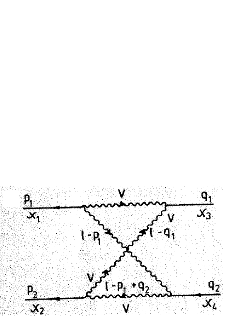
Figure 15:

and the analogous diagram with the opposite vector boson current direction are obtained from the above expression but with the substitution $p_{2}\Leftrightarrow-q_{2}$.

Here,

$$F_{1}=\frac{1}{s^{2}+q_{1}^{4}+q_{2}^{4}-2sq_{1}^{2}-2sq_{2}^{2}-2q_{1}^{2}q_{2}^{2}}\times$$ (2.35)

$$\left\{(t+q_{1}^{2}-p_{1}^{2})\left[(s+q_{1}^{2}-q_{2}^{2})(q_{1}^{2}-q_{2}^{2})-2sq_{1}^{2}\right]+q_{1}^{2}(p_{2}^{2}-p_{1}^{2}+q_{1}^{2}-q_{2}^{2})(s+q_{2}^{2}-q_{1}^{2})\right\}$$

$$F_{2}=\frac{1}{s^{2}+p_{1}^{4}+p_{2}^{4}-2sp_{1}^{2}-2sp_{2}^{2}-2p_{1}^{2}p_{2}^{2}}\times$$ (2.36)

$$\left\{(t+p_{1}^{2}-q_{1}^{2})\left[(s+p_{1}^{2}-p_{2}^{2})(p_{1}^{2}-p_{2}^{2})-2sp_{1}^{2}\right]+p_{1}^{2}(p_{1}^{2}-p_{2}^{2}+q_{2}^{2}-q_{1}^{2})(s+p_{2}^{2}-p_{1}^{2})\right\}$$

$$F_{3}=\frac{1}{t+p_{1}^{4}+q_{1}^{4}-2p_{1}^{2}q_{1}^{2}-2tp_{1}^{2}-2tq_{1}^{2}}\times$$ (2.37)

$$\left\{(s+q_{1}^{2}-q_{2}^{2})\left[(t+q_{1}^{2}-p_{1}^{2})(q_{1}^{2}-p_{1}^{2})-2tq_{1}^{2}\right]+q_{1}^{2}(p_{2}^{2}-p_{1}^{2}+q_{1}^{2}-q_{2}^{2})(t+p_{1}^{2}-q_{1}^{2})\right\}$$

$$F_{4}=\frac{1}{t^{2}+p_{2}^{4}+q_{2}^{4}-2tp_{2}^{2}-2tq_{2}^{2}-2p_{2}^{2}q_{2}^{2}}\times$$ (2.38)

$$\left\{(s+q_{2}^{2}-q_{1}^{2})\left[(t+q_{2}^{2}-p_{2}^{2})(q_{2}^{2}-p_{2}^{2})-2tq_{2}^{2}\right]+q_{2}^{2}(p_{1}^{2}-p_{2}^{2}+q_{2}^{2}-q_{1}^{2})(t+q_{2}^{2}-p_{2}^{2})\right\}$$

$$F_{5} = \frac{(t+q_{1}^{2}-p_{1}^{2})(s+q_{1}^{2}-q_{2}^{2})+2q_{1}^{2}(p_{1}^{2}-p_{2}^{2}+q_{2}^{2}-q_{1}^{2})}{s^{2}+q_{1}^{4}+q_{2}^{4}-2sq_{1}^{2}-2sq_{2}^{2}-2q_{1}^{2}q_{2}^{2}}$$ (2.39)

$$F_{6} = \frac{(s+q_{1}^{2}-q_{2}^{2})(t+q_{1}^{2}-p_{1}^{2})+2q_{1}^{2}(p_{1}^{2}-p_{2}^{2}+q-2^{2}-q_{1}^{2})}{t^{2}+p_{1}^{4}+q_{1}^{4}--2tp_{1}^{2}-2tq_{1}^{2}-2p_{1}^{2}q_{1}^{2}}$$ (2.40)

$$F_{7} = \frac{(t+q_{1}^{2}-p_{1}^{2})(s+q_{2}^{2}-q_{1}^{2})+(p_{1}^{2}-p_{2}^{2}+q_{2}^{2}-q_{1}^{2})(s-q_{1}^{2}-q_{2}^{2})}{s^{2}+q_{1}^{4}+q_{2}^{4}-2sq_{1}^{2}-2sq_{2}^{2}-2q_{1}^{2}q_{2}^{2}}$$

$$F_{8} = \frac{(s+q_{2}^{2}-q_{1}^{2})(t+q_{2}^{2}-p_{2}^{2})+2q_{2}^{2}(p_{2}^{2}-p_{1}^{2}+q_{1}^{2}-q_{2}^{2})}{t^{2}+p_{2}^{4}+q_{2}^{4}-2tp_{2}^{2}-2tq_{2}^{2}-2p_{2}^{2}q_{2}^{2}}$$ (2.42)

$$F_{9} = \frac{(t+p_{1}^{2}-q_{1}^{2})(s+p_{1}^{2}-p_{2}^{2})+2p_{1}^{2}(p_{2}^{2}-p_{1}^{2}+q_{1}^{2}-q_{2}^{2})}{s^{2}+p_{1}^{4}+p_{2}^{4}-2sp_{1}^{2}-2sp_{2}^{2}-2p_{1}^{2}p_{2}^{2}}$$ (2.43)

$$F_{10} = \frac{(s+q_{1}^{2}-q_{2}^{2})(t+p_{1}^{2}-q_{1}^{2})+(t-q_{1}^{2}-p_{1}^{2})(p_{2}^{2}-p_{1}^{2}+q_{1}^{2}-q_{2}^{2})}{t^{2}+p_{1}^{4}+q_{1}^{4}-2tp_{1}^{2}-2tq_{1}^{2}-2p_{1}^{2}q_{1}^{2}}$$

$$F_{11} = \frac{(t+p_{1}^{2}-q_{1}^{2})(s+p_{2}^{2}-p_{1}^{2})+(s-p_{1}^{2}-p_{2}^{2})(p_{2}^{2}-p_{1}^{2}+q_{1}^{2}-q_{2}^{2})}{s^{2}+p_{1}^{4}+p_{2}^{4}-2sp_{1}^{2}-2sp_{2}^{2}-2p_{1}^{2}p_{2}^{2}}$$

$$F_{12} = \frac{(s+q_{2}^{2}-q_{1}^{2})(t+p_{2}^{2}-q_{2}^{2})+(t-p_{2}^{2}-q_{2}^{2})(p_{2}^{2}-p_{1}^{2}+q_{1}^{2}-q_{2}^{2})}{t^{2}+p_{2}^{4}+q_{2}^{4}-2tp_{2}^{2}-2tq_{2}^{2}-2p_{2}^{2}q_{2}^{2}}$$

$$F_{13} = \frac{-2s(t+q_{1}^{2}-p_{1}^{2})+(s+q_{1}^{2}-q_{2}^{2})(p_{1}^{2}-p_{2}^{2}+q_{2}^{2}-q_{1}^{2})}{s^{2}+q_{1}^{4}+q_{2}^{4}-2sq_{1}^{2}-2sq_{2}^{2}-2q_{1}^{2}q_{2}^{2}}$$ (2.47)

$$F_{14} = \frac{-2s(t+p_{1}^{2}-q_{1}^{2})+(s+p_{1}^{2}-p_{2}^{2})(p_{1}^{2}-p_{2}^{2}+q_{2}^{2}-q_{1}^{2})}{s^{2}+p_{1}^{4}+p_{2}^{4}-2sp_{1}^{2}-2sp_{2}^{4}-2p_{1}^{2}p_{2}^{2}}$$ (2.48)

$$F_{15} = \frac{-2t(s+q_{1}^{2}-q_{2}^{2})+(t+q_{1}^{2}-p_{1}^{2})(p_{1}^{2}-p_{2}^{2}+q_{2}^{2}-q_{1}^{2})}{t^{2}+p_{1}^{4}+q_{1}^{4}-2tp-1^{2}-2tq_{1}^{2}-2q_{1}^{2}q_{2}^{2}}$$ (2.49)

$$F_{16} = \frac{-2t(s+q_{2}^{2}-q_{1}^{2})+(t+q_{2}^{2}-p_{2}^{2})(p_{1}^{2}-p_{2}^{2}+q_{2}^{2}-q_{1}^{2})}{t^{2}+p_{2}^{4}+q_{2}^{4}-2tp_{2}^{2}-2tq_{2}^{2}-2p_{2}^{2}q_{2}^{2}}$$ (2.50)

and

$$p_{1}p_{2} = {1\over 2}\left(s-p_{1}^{2}-p_{2}^{2}\right),\qquad p_{1}q_{2}={1\over 2}\left(s+t-p_{2}^{2}-q_{1}^{2}\right),$$

$$q_{1}q_{2} = {1\over 2}\left(s-q_{1}^{2}-q_{2}^{2}\right),\qquad p_{2}q_{1}={1\over 2}\left(s+t-p_{1}^{2}-q_{2}^{2}\right),$$

$$p_{1}q_{1} = -{1\over 2}\left(t-p_{1}^{2}-q_{1}^{2}\right),$$

$$p_{2}q_{2} = -{1\over 2}\left(t-p_{2}^{2}-q_{2}^{2}\right)$$ (2.51)

with $s,t,u$ being the Mandelstam variables. $I_{0},I_{1},I_{2}$ are the scalar one-loop integrals calculated in [15].

3 The one-loop amplitudes.

The box diagrams of the previous Section and the diagrams drawn at Fig. 16 (see also [13b]) contribute to the Higgs-Higgs amplitude up to fourth order of perturbation theory to give

$$i{\cal M}_{a} = {9ig^{2}\over 4}r_{W}{M_{\chi}^{2}\over t+M_{\chi}^{2}},$$ (3.52)

$$i{\cal M}_{b,c} = -{3g\over 2}r_{W}\frac{M_{W}\Gamma^{ren}(p^{2}_{1,2},q_{1,2}^{2},t)}{t+M_{\chi}^{2}},$$ (3.53)

$$i{\cal M}_{d,e} = {9g^{2}\over 4}r_{W}\frac{M_{\chi}^{2}\Pi^{ren}(p_{1,2}^{2})}{(p_{1,2}^{2}+M_{\chi}^{2})(t+M_{\chi}^{2})},$$ (3.54)

$$i{\cal M}_{f,g} = {9g^{2}\over 4}r_{W}\frac{M_{\chi}^{2}\Pi^{ren}(q_{1,2}^{2})}{(q_{1,2}^{2}+M_{\chi}^{2})(t+M_{\chi}^{2})},$$ (3.55)

$$i{\cal M}_{h} = {9g^{2}\over 4}r_{W}\frac{M_{\chi}^{2}\Pi^{ren}(t)}{(t+M_{\chi}^{2})^{2}},$$ (3.56)

$$i{\cal M}_{i} = {9g^{4}\over 16}r_{W}^{2}\Pi^{(3)}(t),$$ (3.57)

$$i{\cal M}_{j} = {g^{4}\over 4}\Pi^{(5)}(t)|_{M_{V}^{2}=M_{W}^{2}}+{g^{4}\over 4}{1\over R^{2}}\Pi^{(5)}(t)|_{M_{V}^{2}=M_{Z}^{2}},$$ (3.58)

$$i{\cal M}_{k,l} = -{27\over 16}g^{4}r_{W}^{2}M_{\chi}^{2}\Gamma^{(1)}(p_{1,2}^{2},q_{1,2},t),$$ (3.59)

$$i{\cal M}_{m,n} = -{g^{4}\over 2}M_{W}^{2}\Gamma^{(3)}(p_{1,2}^{2},q_{1,2},t)|_{M_{V}^{2}=M_{W}^{2}}-$$ (3.60)

$$-{g^{4}\over 2}{1\over R^{2}}M_{Z}^{2}\Gamma^{(3)}(p_{1,2}^{2},q_{1,2},t)|_{M_{V}^{2}=M_{Z}^{2}},$$

$$i{\cal M}_{o} = -{3ig^{2}\over 4}r_{W},$$ (3.61)

$$i{\cal M}_{p} = -{3g^{2}\over 4}r_{W}\frac{\Pi^{ren}(p_{1}^{2})}{(p_{1}^{2}+M_{\chi}^{2})},$$ (3.62)

$$i{\cal M}_{r} = -{3g^{2}\over 4}r_{W}\frac{\Pi^{ren}(p_{2}^{2})}{(p_{2}^{2}+M_{\chi}^{2})},$$ (3.63)

$$i{\cal M}_{s} = -{3g^{2}\over 4}r_{W}\frac{\Pi^{ren}(q_{1}^{2})}{(q_{1}^{2}+M_{\chi}^{2})},$$ (3.64)

$$i{\cal M}_{t} = -{3g^{2}\over 4}r_{W}\frac{\Pi^{ren}(q_{2}^{2})}{(q_{2}^{2}+M_{\chi}^{2})}.$$ (3.65)

The digrams describing the interaction of two Higgs particle ($s$-channel)are presnted in [14], a solid line corresponds to the renormalized propagator and a black circle, to the renormalized vertex.

In the framework of the renormalization scheme [10] (using the unitary gauge) the appropriate counterterm for $4\chi$ interaction is written as follows:

$$i{\cal M}^{c.t.}=-{3g^{2}M_{\chi}^{2}\over 4M_{W}^{2}}\left[2(Z_{\chi}-1)+2{\delta g\over g}+{\delta M_{\chi}^{2}\over M_{\chi}^{2}}-{\delta M_{W}^{2}\over M_{W}^{2}}\right].$$ (3.66)

After substitution of the renormalization constants (see preceding Section) we have

$$i{\cal M}^{c.t}(p_{1}^{2},p_{2}^{2},q_{1}^{2},q_{2}^{2},s,t)=-\frac{ig^{4}}{16\pi^{2}}{3r_{W}\over 4}\left\{\left[-{3\over 4}r_{W}-9r_{W}^{-1}-{9\over 2R}r_{Z}^{-1}+\right.\right.$$ (3.67)

$$+ \left.\left.{6\over M_{W}^{2}M_{\chi}^{2}}Tr\,m_{i}^{4}\right]P+{52\over 3}-{56\over 3}R-8R^{2}-{19\over 12R}-{1\over 12R^{2}}+{31\over 8}r_{W}-\right.$$

$$- \left.{1\over 2}r_{W}^{2}+{1\over 2}r_{W}r_{Z}+{21\over 2}r_{W}^{-1}+{21\over 4R}r_{Z}^{-1}+\right.$$

$$+ \left.(-{3\over 8}r_{W}+{3\over 4R}+{9\over 4R}r_{Z}^{-1})\log\,R+{1\over 1-R}(-{47\over 6}+{14\over 3R}-{1\over 2R^{2}}-{1\over 24R^{3}}+\right.$$

$$+ \left.{3\over 4}r_{Z}-{1\over 4}r_{Z}^{2}+{1\over 24}r_{Z}^{3})\log\,R+(-{3\over 4}-{1\over 4}r_{W}+{1\over 4}r_{Z}+{1\over 24}r_{W}^{2}-\right.$$

$$- \left.\left.{1\over 24}r_{W}r_{Z}-{1\over 24}r_{Z}^{2})r_{W}\log\,r_{W}-{20\over 9}(1-R)Tr\,Q_{i}^{2}+\right.\right.$$

$$+ \left.{1\over 2M_{W}^{2}}{R\over 1-R}(-{1\over 12}-{4\over 3}R+{17\over 3}R^{2}+4R^{4})L(-M_{Z}^{2},M_{W}^{2},M_{W}^{2})+\right.$$

$$+ \left.{1\over 2M_{W}^{2}}{R\over 1-R}(-1+{1\over 3}r_{Z}-{1\over 12}r_{Z}^{2})L(-M_{Z}^{2},M_{Z}^{2},M_{\chi}^{2})+\right.$$

$$+ \left.{1\over 2M_{W}^{2}}{1\over 1-R}({25\over 3}-{22\over 3}R-8R^{2}-{7\over 6R}-{1\over 12R^{2}})L(-M_{W}^{2},M_{W}^{2},M_{Z}^{2})+\right.$$

$$+ \left.{1\over 2M_{W}^{2}}{1\over 1-R}\left(-1+2R+{1\over 3}r_{W}-{2\over 3}r_{Z}+\right.\right.$$

$$+ \left.\left.{1\over 6}r_{W}r_{Z}-{1\over 12}r_{W}^{2}\right)L(-M_{W}^{2},M_{W}^{2},M_{\chi}^{2})+\right.$$

$$+ \left.{1\over M_{W}^{2}}(-{3\over 8}+{3\over 2}r_{W}^{-2}-6{1\over r_{W}^{2}(r_{W}-4)})L(-M_{\chi}^{2},M_{W}^{2},M_{W}^{2})+\right.$$

$$+ \left.{1\over M_{W}^{2}}(-{3\over 16}+{3\over 4}r_{Z}^{-2}-3{1\over r_{Z}^{2}(r_{Z}-4)})L(-M_{\chi}^{2},M_{Z}^{2},M_{Z}^{2})+\right.$$

$$+ \left.{21\over 16M_{W}^{2}}L(-M_{\chi}^{2},M_{\chi}^{2},M_{\chi}^{2})+\right.$$

$$+ \left.{1\over M_{W}^{2}}Tr\,\left[{1\over 3}m_{i}^{2}+({8\over 3}|Q_{i}|-{16\over 3}Q_{i}^{2})Rm_{i}^{2}+{16\over 3}Q_{i}^{2}R^{2}m_{i}^{2}\right]+\right.$$

$$+ \left.{1\over M_{W}^{4}}Tr\,\left[{1\over 6}m_{i}^{4}-{1\over 6}{R\over 1-R}m_{i}^{4}-{15\over 2}r_{W}^{-1}m_{i}^{4}\right]+\right.$$

$$- \left.{1\over M_{W}^{2}}Tr\,\left[{1\over 6}{1\over 1-R}M_{W}^{2}-{2\over 3}|Q_{i}|M_{W}^{2}+{1\over 2}(1-{R\over 1-R})m_{i}^{2}+{3\over M_{\chi}^{2}}m_{i}^{4}\right]\times\right.$$

$$\times \left.\log\,{m_{i}^{2}\over M_{W}^{2}}+{1\over M_{W}^{2}}Tr\,\left[-{1\over 12}{R\over 1-R}+({1\over 3}|Q_{i}^{2}|-{2\over 3}Q_{i}^{2})R+{2\over 3}Q_{i}^{2}R^{2}+\right.\right.$$

$$+ \left.\left.{1\over 12}{R\over 1-R}{m_{i}^{2}\over M_{Z}^{2}}+({2\over 3}|Q_{i}|-{4\over 3}Q_{i}^{2})R{m_{i}^{2}\over M_{Z}^{2}}+{4\over 3}Q_{i}^{2}R^{2}{m_{i}^{2}\over M_{Z}^{2}}\right]L(-M_{Z}^{2},m_{i}^{2},m_{i}^{2})-\right.$$

$$- \left.{1\over M_{W}^{2}}Tr\,\left[{m_{i}^{2}\over 4M_{\chi}^{2}}+2{m_{i}^{4}\over M_{\chi}^{4}}\right]L(-M_{\chi}^{2},m_{i}^{2},m_{i}^{2})+({R\over 1-R}-1)\times\right.$$

$$\times \left.\sum_{i\,j}^{N_{f}/2}\left[{1\over 3}{m_{i}^{2}m_{j}^{2}\over M_{W}^{4}}-{1\over 3}-\frac{m_{i}^{2}+m_{j}^{2}}{2M_{W}^{2}})\log\,{m_{i}m_{j}\over M_{W}^{2}}+{1\over 12}{(m_{i}^{2}-m_{j}^{2})^{3}\over M_{W}^{6}}\log\,{m_{i}^{2}\over m_{j}^{2}}+\right.\right.$$

$$+ \left.\left.({1\over 6M_{W}^{2}}-{m_{i}^{2}+m_{j}^{2}\over 12M_{W}^{4}}-{(m_{i}^{2}-m_{j}^{2})^{2}\over 12M_{W}^{6}})L(-M_{W}^{2},m_{i}^{2},m_{j}^{2})\right]K_{ij}K^{+}_{ij}\right\}-$$

$$- {g\over 2M_{W}}\Gamma^{3\chi}(tadpoles)\,.$$

I would also lke to note that it is not useful to use the Stuart’s computer algebra programm [22] since the preparation of the input data for the two-Higgs processes would consume more time than the calculations by hand.

4 Summary.

We calculated the Higgs-Higgs amplitude in the fourth order of perturbation theory (that is, with taking into account the one-loop corrections) in the Standard Model. The results do not coincide in full with the Durand et al. calculations in the Feynman gauge and within the different renormalization scheme [17].

There exists a rather large number of different variants of the SM extensions. The most of these models are characterized by enlarging of the Higgs sector, namely by introduction of two and even more Higgs boson doublets [24]-[26]. The supersymmetric extension of the SM [27, 28] also requires introduction of at least two doublets of the scalar particles. The interest in these models has grown up in connection with the problem of suppression of the $CP$ violation in strong interactions [29] and the problem of $B^{0}\bar{B}^{0}$ mixing [30] because they give the alternative theoretical solution to the problem of electroweak violation of the $CP$ invariance [26, 31]. Therefore, in the approaching paper we are going to consider the Higgs-Higgs interaction problem in the framework of the extended variants of the SM. This is easily possible due to introduction of the parameters $a_{i}$, $b_{i}$ for the fermionic interactions.

Acknowledgements. The author express his sincere gratitude to D. Yu. Bardin, R. N. Faustov, and Yu. N. Tyukhtyaev for valuable discussions. I appreciate very much the assistance of V. I. Kikot’ in calculations, E. Saucedo for technical help, and I thank N. B. Skachkov for putting forward the problem.

Appendix.

The integrals $I_{0}$, $I_{1}$ and $I_{2}$ are taken from the t’Hooft-Veltman paper [15]

$$I_{0}(q^{2},M_{1}^{2},M_{2}^{2})=\int_{0}^{1}dx\log\,\frac{q^{2}x(1-x)+M_{1}^{2}x+M_{2}^{2}(1-x)}{M_{W}^{2}}=$$ (4.68)

$$= -2+\log{M_{1}M_{2}\over M_{W}^{2}}-{1\over 2}{M_{1}^{2}-M_{2}^{2}\over q^{2}}\log{M_{1}^{2}\over M_{2}^{2}}+{1\over 2q^{2}}L(q^{2},M_{1}^{2},M_{2}^{2})$$

where

$$L(q^{2},M_{1}^{2},M_{2}^{2})=\left[(q^{2}+M_{1}^{2}+M_{2}^{2})-\right.$$ (4.69)

$$- \left.4M_{1}^{2}M_{2}^{2}\right]\int_{0}^{1}\frac{dx}{q^{2}x(1-x)+M_{1}^{2}x+M_{2}^{2}(1-x)},$$

see Ref. [9a,p.440].

Next,

$$I_{1}(q^{2},(p-q)^{2},p^{2},M_{1}^{2},M_{2}^{2},M_{3}^{2}) = \int^{1}_{0}dx\int_{0}^{x}dy\left[ax^{2}+by^{2}+cxy+\right.$$ (4.70)

$$+ \left.dx+ey+f\right]^{-1},$$

with
$a=-(p-q)^{2}$, $d=M_{2}^{2}-M_{3}^{2}+(p-q)^{2}$ $b=-q^{2}$, $e=M_{1}^{2}-M_{2}^{2}+2pq-q^{2}$ $c=-2(pq-q^{2})$, $f=M_{3}^{2}-i\epsilon$.

And,

$$I_{2}(q_{1}^{2},q_{2}^{2},p_{2}^{2},p_{1}^{2},s,t,M_{1}^{2},M_{2}^{2},M_{3}^{2},M_{4}^{2})=$$

$$= \int_{0}^{1}dx\int_{0}^{x}dy\int_{0}^{y}dz\left[ax^{2}+by^{2}+gz^{2}+cxy+hxz+jyz+\right.$$

$$+ \left.dx+ey+kz+f\right]^{-2},$$

with
$a=-p_{2}^{2}$, $f=M_{4}^{2}-i\epsilon$ $b=-q_{2}^{2}$, $g=-q_{1}^{2}$ $c=2p_{2}q_{2}$, $h=2p_{2}q_{1}$ $d=M_{3}^{2}-M_{4}^{2}+p_{2}^{2}$, $j=-2q_{1}q_{2}$ $e=M_{2}^{2}-M_{3}^{2}+q^{2}-2p_{2}q_{2}$, $k=M_{1}^{2}-M_{2}^{2}+q_{1}^{2}+2q_{1}q_{2}-2q_{1}p_{2}$.

The traces of $\gamma$- matrices in an $d$-dimensional space are

$$Tr\,\gamma_{\alpha}=Tr\,\gamma_{5}=Tr\,\gamma_{\alpha}\gamma_{\beta}\gamma_{5}=0,$$ (4.72)

$$Tr\,\gamma_{\alpha}\gamma_{\beta}=f(d)\delta_{\alpha\beta},$$ (4.73)

$$Tr\,\gamma_{\alpha}\gamma_{\beta}\gamma_{\rho}\gamma_{\sigma}=f(d)d_{\alpha\beta\rho\sigma},$$ (4.74)

$$Tr\,\gamma_{\alpha}\gamma_{\beta}\gamma_{\rho}\gamma_{\sigma}\gamma_{5}=f(d)\epsilon_{\alpha\beta\rho\sigma},$$ (4.75)

where

$$d_{\alpha\beta\rho\sigma}=\delta_{\alpha\beta}\delta_{\rho\sigma}-\delta_{\alpha\rho}\delta_{\beta\sigma}+\delta_{\alpha\sigma}\delta_{\beta\rho}.$$ (4.76)

In the present work we use $f(d)=2\omega=4-2\epsilon$, $d$ is the dimension of the space in the dimensional regularization.