Monotonicity-based regularization for phantom experiment data in Electrical Impedance Tomography

Abstract

In electrical impedance tomography, algorithms based on minimizing the linearized-data-fit residuum have been widely used due to their real-time implementation and satisfactory reconstructed images. However, the resulting images usually tend to contain ringing artifacts. In this work, we shall minimize the linearized-data-fit functional with respect to a linear constraint defined by the monotonicity relation in the framework of real electrode setting. Numerical results of standard phantom experiment data confirm that this new algorithm improves the quality of the reconstructed images as well as reduce the ringing artifacts.

1 Introduction

Electrical Impedance Tomography (EIT) is a recently developed non-invasive imaging technique, where the inner structure of a reference object can be recovered from the current and voltage measurements on the object’s surface. It is fast, inexpensive, portable and requires no ionizing radiation. For these reasons, EIT qualifies for continuous real time visualization right at the bedside.

In clinical EIT applications, the reconstructed images are usually obtained by minimizing the linearized-data-fit residuum [7, 1]. These algorithms are fast and simple. However, to the best of the authors’ knowledge, there is no rigorous global convergence results that have been proved so far. Moreover, the reconstructed images usually tend to contain ringing artifacts.

Recently, Seo and one of the author have shown in [20] that a single linearized step can give the correct shape of the conductivity contrast. This result raises a question that whether to regularize the linearized-data-fit functional such that the corresponding minimizer yields a good approximation of the conductivity contrast. An affirmative answer has been proved in [19] for the continuum boundary data. In the present paper, we shall apply this new algorithm to the real electrode setting and test with standard phantom experiment data. Numerical results later on show that this new algorithm helps to improve the quality of the reconstructed images as well as reduce the ringing artifacts. It is worth to mention that our new algorithm is non-iterative, hence, it does not depend on an initial guess and does not require expensive computation. Other non-iterative algorithms, for example, the Factorization Method [15, 16] and the Monotonicity-based Method [31, 30, 22, 4], on the other hand, are much more sensitive to measurement errors than our new algorithm when phantom data or real data are applied [5, 21, 33, 10].

The paper is organized as follows. In Section 2 we introduce the mathematical setting, describe how the measured data can be collected and set up a link between the mathematical setting and the measured data. Section 3 presents our new algorithm and the numerical results were shown in Section 4. We conclude this paper with a brief discussion in Section

2 Mathematical setting

Let $\Omega\subseteq\mathbbm{R}^{n},n\geq 2$ describe the imaging subject and $\sigma:\Omega\to\mathbbm{R}$ be the unknown conductivity distribution inside $\Omega$. We assume that $\Omega$ is a bounded domain with smooth boundary $\partial\Omega$ and that the function $\sigma$ is real-valued, strictly positive and bounded. Electrical Impedance Tomography (EIT) aims at recovering $\sigma$ using voltage and current measurements on the boundary of $\Omega$. There are several ways to inject currents and measure voltages. We shall follow the Neighboring Method (aka Adjacent Method) which was suggested by Brown and Segar in 1987 [6] and is still widely being used by practitioners. In this method, electrodes are attached on the object’s surface, and an electrical current is applied through a pair of adjacent electrodes whilst the voltage is measured on all other pairs of adjacent electrodes excluding those pairs containing at least one electrode with injected current. Figure 1 illustrates the first and second current patterns for a $16$-electrode EIT system. At the first current pattern (figure 1a), small currents of intensity $I^{(1)}_{1}$ and $I^{(1)}_{2}=-I^{(1)}_{1}$ are applied through electrodes $E_{1}$ and $E_{2}$ respectively, and the voltage differences $U^{(1)}_{3},U^{(1)}_{4},\dots,U^{(1)}_{15}$ are measured successively on electrode pairs $(E_{3},E_{4}),(E_{4},E_{5}),\ldots,(E_{15},E_{16})$. In general, for a $L$-electrode EIT system, at the $k$-th current pattern, by injecting currents $I^{(k)}_{k}$ and $I^{(k)}_{k+1}=-I^{(k)}_{k}$ to electrodes $E_{k}$ and $E_{k+1}$ respectively, one gets $L-3$ voltage measurements $\{U^{(k)}_{l}\}$, where $l\in\{1,2,\dots,L\}$ and $|k-l|>1$. Note that here and throughout the paper, the electrode index is always considered modulo $L$, i.e. the index $L+1$ also refers to the first electrode, etc.

Figure 1: The Neighboring Method: a) first current pattern, b) second current pattern.

Assuming that the electrodes $E_{l}$ are relatively open and connected subsets of $\partial\Omega$, that they are perfectly conducting and that contact impedances are negligible, the resulting electric potential $u^{(k)}$ at the $k$-th current pattern obeys the following mathematical model (the so-called shunt model [8]):

$$\begin{array}[]{lllll}&\nabla\cdot(\sigma\nabla u)&=&0&\mbox{ in }\Omega,\\ &\int_{E_{l}}\sigma\partial_{\nu}u\;{\rm d}s&=&I^{(k)}_{l}&\mbox{ for }l=1,\dots,L,\\ &\sigma\partial_{\nu}u&=&0&\mbox{ on }\partial\Omega\setminus\bigcup_{l=1}^{L}E_{l},\\ &u|_{E_{l}}&=&\mbox{const.}&\mbox{ for }l=1,\dots,L.\end{array}$$ (5)

Here $\nu$ is the unit normal vector on $\partial\Omega$ pointing outward and $I^{(k)}_{l}:=(\delta_{k,l}-\delta_{k+1,l})I$ describes the $k$-th applied current pattern where a current of strength $I>0$ is driven through the $k$-th and $(k+1)$-th electrode. Notice that $\{I^{(k)}_{l}\}$ satisfy the conservation of charge $\sum_{l=1}^{L}I^{(k)}_{l}=0$, and that the electric potential $u^{(k)}$ is uniquely determined by (5) only up to the addition of a constant. The voltage measurements are given by

$$U^{(k)}_{l}:=u^{(k)}|_{E_{l}}-u^{(k)}|_{E_{l+1}}.$$ (6)

The herein used shunt model ignores the effect of contact impedances between the electrodes and the imaging domain. This is only valid when voltages are measured on small (see [14]) and current-free electrodes, so that (5) correctly models only the measurements $U^{(k)}_{l}$ with $|k-l|>1$. For difference measurements, the missing elements $U^{(k)}_{l}$ with $|k-l|\leq 1$, on the other hand, can be calculated by interpolation taking into account reciprocity, conservation of voltages and the geometry-specific smoothness of difference EIT data, cf. [17]. For an imaging subject with unknown conductivity $\sigma$, one thus obtains a full matrix of measurements $U(\sigma)=(U^{(k)}_{l})_{k,l=1,\ldots,L}$.

3 Monotonicity-based regularization

3.1 Standard one-step linearization methods

In difference EIT, the measurements $U(\sigma)$ are compared with measurements $U(\sigma_{0})$ for some reference conductivity distribution $\sigma_{0}$ in order to reconstruct the conductivity difference $\sigma-\sigma_{0}$. This is usually done by a single linearization step

$$U^{\prime}(\sigma_{0})(\sigma-\sigma_{0})\approx U(\sigma)-U(\sigma_{0}).$$

where $U^{\prime}(\sigma_{0}):L^{\infty}(\Omega)\to\mathbbm{R}^{L\times L}$ is the Fréchet derivative of the voltage measurements

$$U^{\prime}(\sigma_{0}):\kappa\mapsto\left(-\int_{\Omega}\kappa\nabla u^{(k)}_{\sigma_{0}}\cdot\nabla u^{(l)}_{\sigma_{0}}\,{\rm d}x\right)_{1\leq k,l\leq L}$$

We discretize the reference domain $\overline{\Omega}=\cup_{j=1}^{P}\overline{P}_{j}$ into $P$ disjoint open pixels $P_{j}$ and make the piecewise-constant Ansatz

$$\kappa(x)=\sum_{j=1}^{P}\kappa_{j}\chi_{P_{j}}(x).$$

This approach leads to the linear equation

$$\mathbf{S}\mathbf{\kappa}=\mathbf{V}$$ (7)

where $\mathbf{V}$ and the columns of the sensitivity matrix $\mathbf{S}$ contain the entries of the measurements $U(\sigma)-U(\sigma_{0})$ and the discretized Fréchet derivative, resp., written as long vectors, i.e.,

$$\mathbf{\kappa}=(\kappa_{j})_{j=1}^{P}\in\mathbbm{R}^{P},$$

$$\mathbf{V}=(V_{i})_{i=1}^{L^{2}}\in\mathbbm{R}^{L^{2}},\quad\mbox{ with }V_{(l-1)L+k}=U_{l}^{(k)}(\sigma)-U_{l}^{(k)}(\sigma_{0}),$$

$$\mathbf{S}=(S_{i,j})\in\mathbbm{R}^{L^{2},P},\quad\mbox{ with }S_{(l-1)L+k,j}=-\int_{P_{j}}\nabla u^{(k)}_{\sigma_{0}}\cdot\nabla u^{(l)}_{\sigma_{0}}\,{\rm d}x.$$

Most practically used EIT algorithms are based on solving a regularized variant of (7) to obtain an approximation $\kappa$ to the conductivity difference $\sigma-\sigma_{0}$. The popular algorithms NOSER [7] and GREIT [1] use (generalized) Tikhonov regularization and minimize

$$\hskip 0.86108pt\|\mathbf{S}\mathbf{\kappa}-\mathbf{V}\|\hskip 0.86108pt^{2}_{\mathrm{res}}+\alpha\hskip 0.86108pt\|\mathbf{\kappa}\|\hskip 0.86108pt^{2}_{\mathrm{pen}}\to\mbox{min!}$$

with (heuristically chosen) weighted Euclidian norms $\hskip 0.86108pt\|\cdot\|\hskip 0.86108pt_{\mathrm{res}}$ and $\hskip 0.86108pt\|\cdot\|\hskip 0.86108pt_{\mathrm{pen}}$ in the residuum and penalty term.

3.2 Monotonicity-based regularization

It has been shown in [20] that shape information in EIT is invariant under linearization. Thus one-step linearization methods are principally capable of reconstructing the correct (outer) support of the conductivity difference even though they ignore the non-linearity of the EIT measurement process. In [19] the authors developed a monotonicity-based regularization method for the linearized EIT equation for which (in the continuum model) it can be guaranteed that the regularized solutions converge against a function that shows the correct outer shape. In this section, we formulate and analyze this new method for real electrode measurements, and in the next section we will apply it to real data from a phantom experiment and compare it with the GREIT method.

The main idea of monotonicity-based regularization is to minimize the residual of the linearized equation (7)

$$\hskip 0.86108pt\|\mathbf{S}\mathbf{\kappa}-\mathbf{V}\|\hskip 0.86108pt^{2}\to\mbox{min!}$$

with constraints on the entries of $\mathbf{\kappa}$ that are obtained from monotonicity tests.

For the following, we assume that the background is homogeneous and that all anomalies are more conductive, or all anomalies are less conductive than the background, i.e., $\sigma_{0}$ is constant, and either

$$\sigma(x)=\sigma_{0}+\gamma(x)\chi_{D}(x),\quad\mbox{ or }\quad\sigma(x)=\sigma_{0}-\gamma(x)\chi_{D}(x).$$

$D$ is an open set denoting the conductivity anomalies, and $\gamma:\ D\to\mathbbm{R}$ is the contrast of the anomalies. We furthermore assume that we are given a lower bound $c>0$ of the anomaly contrast, i.e. $\gamma(x)\geq c$.

For the monotonicity tests it is crucial to consider the measurements and the columns of the sensitivity matrix $\mathbf{S}$ as matrices and compare them in terms of matrix definiteness, cf. [9, 23, 17] for the origins of this sensitivity matrix based approach. Let $V:=U(\sigma)-U(\sigma_{0})\in\mathbbm{R}^{L\times L}$ denote the EIT difference measurements written as $L\times L$-matrix, and $S_{k}\in\mathbbm{R}^{L\times L}$ denote the $k$-th column of the sensitivity matrix written as $L\times L$-matrix, i.e. the $(j,l)$-th entry of $S_{k}$ is given by

$$-\int_{P_{k}}\nabla u^{(j)}_{\sigma_{0}}\cdot\nabla u^{(l)}_{\sigma_{0}}\,{\rm d}x.$$

We then define for each pixel $P_{k}$

$$\beta_{k}:=\max\{\alpha\geq 0:\alpha S_{k}\geq-|V|\},$$ (8)

where $|V|$ denotes the matrix absolute value of $V$, and the comparison $\alpha S_{k}\geq-|V|$ is to be understood in the sense of matrix definiteness, i.e. $\alpha S_{k}\geq-|V|$ holds if and only if all eigenvalues of $\alpha S_{k}+|V|$ are non-negative.

Following [19] we then solve the linearized EIT equation (7) using the monotonicity constraints $\beta_{k}$. We minimize the Euclidean norm of the residuum

$$\hskip 0.86108pt\|\mathbf{S}\mathbf{\kappa}-\mathbf{V}\|\hskip 0.86108pt^{2}\to\mbox{min!}$$ (9)

under the constraints that

1. in the case $\sigma\geq\sigma_{0}$: $0\leq\kappa_{k}\leq\min(a_{+},\beta_{k})$, and

2. in the case $\sigma\leq\sigma_{0}$: $0\geq\kappa_{k}\geq-\min(a_{-},\beta_{k})$.

where $a_{+}:=\sigma_{0}-\frac{\sigma_{0}^{2}}{\sigma_{0}+c}$, and $a_{-}:=c$.

For noisy data $V^{\delta}$ with $\hskip 0.86108pt\|V^{\delta}-V\|\hskip 0.86108pt\leq V$ this approach can be regularized by replacing $\beta_{k}$ with

$$\beta_{k}^{\delta}:=\max\{\alpha\geq 0:\alpha S_{k}\geq-|V|-\delta I\},$$ (10)

where $I\in\mathbbm{R}^{L\times L}$ is the identity matrix. For the implementation of $\beta_{k}^{\delta}$ see section 4.

For the continuum model, and under the assumption that $D$ has connected complement, the authors [19] showed that for exact data this monotonicity-constrained minimization of the linearized EIT residuum admits a unique solution and that the support of the solution agrees with the anomalies support $D$ up to the pixel partition. Moreover, [19] also shows that for noisy data and using the regularized constraints $\beta_{k}^{\delta}$, minimizers exist and that, for $\delta\to 0$, they converge to the minimizer with the correct support. Since practical electrode measurements can be regarded as an approximation to the continuum model, we therefore expect that the above approach will also well approximate the anomaly support for real electrode data.

In the continuum model, the constraints $\beta_{k}$ will be zero outside the support of the anomaly and positive for each pixel inside the anomaly. The first property relies on the existence of localized potentials [11] and is only true in the limit of infinitely many, infinitely small electrodes. The latter property is however true for any number of electrodes as the following result shows:

Theorem 3.1.

If $P_{k}\subseteq D$, then

1. in the case $\sigma\geq\sigma_{0}$ the constraint $\beta_{k}$ fulfills $\beta_{k}\geq a_{+}>0$, and

2. in the case $\sigma\leq\sigma_{0}$ the constraint $\beta_{k}$ fulfills $\beta_{k}\geq a_{-}>0$.

Proof.

If $P_{k}\subseteq D$ and $\sigma\geq\sigma_{0}$ then

$$\frac{\sigma_{0}}{\sigma}(\sigma-\sigma_{0})=\sigma_{0}-\frac{\sigma_{0}^{2}}{\sigma}\geq\left(\sigma_{0}-\frac{\sigma_{0}^{2}}{\sigma_{0}+c}\right)\chi_{P_{k}}=a_{+}\chi_{P_{k}},$$

and if $P_{k}\subseteq D$ and $\sigma\leq\sigma_{0}$ then

$$\sigma_{0}-\sigma\geq cP_{k}=a_{-}P_{k}.$$

Hence, it suffices to show that $\alpha S_{k}\geq-|V|$ holds for all $\alpha>0$ that fulfill

1. $\alpha\chi_{P_{k}}\leq\frac{\sigma_{0}}{\sigma}(\sigma-\sigma_{0})$, or

2. $\alpha\chi_{P_{k}}\leq\sigma_{0}-\sigma$.

We use the following monotonicity relation from [18, Lemma 3.1] (see also [25, 24] for the origin of this estimate): For any vector $g=(g_{j})_{j=1}^{L}\in\mathbbm{R}^{L}$ we have that

$$\int_{\Omega}\frac{\sigma_{0}}{\sigma}(\sigma_{0}-\sigma)\left|\nabla u^{(g)}_{\sigma_{0}}\right|^{2}{\rm d}x\geq g^{\top}Vg\geq\int_{\Omega}(\sigma_{0}-\sigma)\left|\nabla u^{(g)}_{\sigma_{0}}\right|^{2}{\rm d}x,$$ (11)

with $u^{(g)}_{\sigma_{0}}=\sum_{j=1}^{L}g_{j}\nabla u^{(j)}_{\sigma_{0}}$.

If $\alpha\chi_{P_{k}}\leq\frac{\sigma_{0}}{\sigma}(\sigma-\sigma_{0})$, then

$$0\geq g^{\top}(\alpha S_{k})g=-\int_{P_{k}}\alpha\left|\nabla u^{(g)}_{\sigma_{0}}\right|^{2}\geq\int_{\Omega}\frac{\sigma_{0}}{\sigma}(\sigma_{0}-\sigma)\left|\nabla u^{(g)}_{\sigma_{0}}\right|^{2}\geq g^{\top}Vg,$$

which shows that $|V|=-V\geq-\alpha S_{k}$.

If $\alpha\chi_{P_{k}}\leq\sigma_{0}-\sigma$, then

$$0\leq g^{\top}(-\alpha S_{k})g=\int_{P_{k}}\alpha\left|\nabla u^{(g)}_{\sigma_{0}}\right|^{2}\leq\int_{\Omega}(\sigma_{0}-\sigma)\left|\nabla u^{(g)}_{\sigma_{0}}\right|^{2}\leq g^{\top}Vg,$$

which shows that $|V|=V\geq-\alpha S_{k}$. ∎

4 Numerical results

In this section, we will test our algorithm on the data set iirc$\_$data$\_$2006 measured by Professor Eung Je Woo’s EIT research group in Korea [32, 26, 28, 27]. iirc stands for Impedance Imaging Research Center. The data set iirc$\_$data$\_$2006 is publicly available as part of the open source software framework EIDORS [3] (Electrical Impedance and Diffused Optical Reconstruction Software). Since iirc$\_$data$\_$2006 is also frequently used in the EIDORS tutorials, we believe that this is a good benchmark example to test our new algorithm.

4.1 Experiment setting

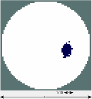
The data set iirc$\_$data$\_$2006 was collected using the 16-electrode EIT system KHU Mark1 (see [29] for more information of this system). The reference object was a Plexiglas tank filled with saline. The tank was a cylinder of diameter 0.2m with 0.01m diameter round electrodes attached on its boundary. Saline was filled to about 0.06m depth. Inside the tank, one put a Plexiglas rod of diameter 0.02m. The conductivity of the saline was 0.15 S/m and the Plexiglas rod was basically non-conductive. Data acquisition protocol was adjacent stimulation, adjacent measurement with data acquired on all electrodes.

The data set iirc$\_$data$\_$2006 contains the voltage measurements for both homogeneous and non-homogeneous cases. Measurements for the homogeneous case were obtained when the Plexiglas rod was taken away (reference conductivity in this case is 0.15 S/m). In the non-homogeneous case, $100$ different voltage measurements were measured corresponding to $100$ different positions of the Plexiglas rod.

4.2 Numerical implementation

EIDORS [3] (Electrical Impedance and Diffused Optical Reconstruction Software) is an open source software that is widely used to reconstruct images in electrical impedance tomography and diffuse optical tomography. To reconstruct images with EIDORS, one first needs to build an EIDORS model that fits with the measured data. In this paper, we shall use the same EIDORS model described in the EIDORS tutorial web-page:

http://eidors3d.sourceforge.net/tutorial/EIDORS_basics/tutorial110.shtml

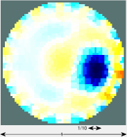
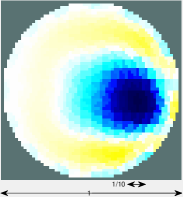
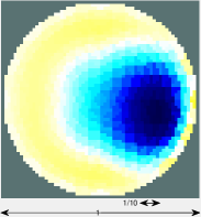
Figure 2 shows the reconstructed images of the $9$th-inhomogeneous measurements with different regularization parameters using the EIDORS built-in command inv$\_$solve, which follows the algorithm proposed in [2]. We emphasize that, Figure 2(b) (regularization parameter is chosen as $0.03$ by default) was considered at the EIDORS tutorial web-page, we show them here again in order to easily compare them with the reconstructed images using our new method later on.

((a)) Parameter $=0.003$

((b)) Parameter $=0.03$

((c)) Parameter $=0.3$

Figure 2: Reconstructed images for the $9$th-inhomogeneous voltage measurements with different regularization parameters.

4.3 Minimizing the residuum

In the EIDORS model suggested in the EIDORS tutorial web-page, the reference body was chosen by default as a disk of diameter $1$m and the default reference conductivity was $1$ S/m. However, in the experiment setting, the reference body was a cylinder of diameter $0.2$m and the reference conductivity was $0.15$ S/m. Hence, an appropriate scaling factor should be applied to the measurements, to make sure that the EIDORS model fits with these measurements. In the EIDORS tutorial web-page, the measurements were scaled by multiplying by a factor $10^{-4}$. In this paper, to increase the precision of the model, we shall find the best scaling factor that minimizes the error between the measured data and the data generated by the EIDORS model. More precisely, let call vh the measured data for homogeneous case and vh$\_$model the homogeneous data generated by the EIDORS model, the best scaling factor is a minimizer of the following problem

$$\min_{c\in\mathbbm{R}}\|c*\texttt{vh}-\texttt{vh$\_$model}\|_{2}$$

For this experiment setting, the best factor is $2.49577*10^{-5}$. From now on, by measured data we always refer to scaled measured data with respect to this best factor.

((a)) cvx

((b)) quadprog

((c)) EIDORS inv$\_$solve

((d)) GREIT

Figure 3: Reconstructed images for the $9$th-inhomogeneous voltage measurements with different algorithms (after scaling the measured data w.r.t the best scaling factor).

The next step is to recover the missing measurements on the driving electrodes. We shall follow the result in [17] to obtain an approximation for these missing measurements using interpolation.

Now we are in a position to minimize the problem (9) under the linear constraint (C1) or (C2). To do this, we need to clarify ${\it a_{+},a_{-}},$ and $\beta_{k}$ in the linear constraints. After scaling, the reference conductivity is $\sigma_{0}=1$ S/m, and $D$ still denotes the Plexiglas rod with conductivity $\sigma=0$ S/m. Thus, $\gamma=1$, ${\it a}_{-}=\inf_{D}\gamma=1$ and $\beta_{k}$ is calculated using (8). In practice, there is no way to obtain the exact value of the matrix $V$ in (8). Indeed, what we know is just the measured data $V^{\delta}=U^{\delta}(\sigma)-U^{\delta}(\sigma_{0})$, where $\delta$ denotes the noise level. When replacing $|V|$ by the noisy version $|V^{\delta}|$, it may happen that there is no $\alpha>0$ so that the matrix $|V^{\delta}|+\alpha S_{k}$ is still positive semi-definite. Therefore, instead of using (8), we shall calculate $\beta_{k}$ from

$$\beta_{k}=\max\{\alpha\geq 0\;:\;|V^{\delta}|+\alpha S_{k}\geq-\delta I\}.$$

Here, $I$ represents the identity matrix, and $\delta$ is chosen as the absolute value of the smallest eigenvalue of $V^{\delta}$. Notice that, in the presence of noise, $|V^{\delta}|+\delta I$ plays the role of the positive semi-definite matrix $|V|$. We shall follow the argument in [19] to calculate $\beta_{k}$. Let $L$ be the lower triangular Cholesky decomposition matrix of $|V^{\delta}|+\delta I$, and let $\lambda_{s}(L^{-1}S_{k}(L^{*})^{-1})$ be the smallest eigenvalue of the matrix $L^{-1}S_{k}(L^{*})^{-1}$. Since $S_{k}$ is negative semi-definite, so is $L^{-1}S_{k}(L^{*})^{-1}$. Thus, $\lambda_{s}(L^{-1}S_{k}(L^{*})^{-1})\leq 0$. Arguing in the same manner as in [19], we get

$$\beta_{k}=-\frac{1}{\lambda_{s}(L^{-1}S_{k}(L^{*})^{-1})}\geq 0.$$

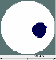
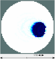
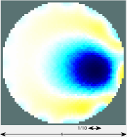
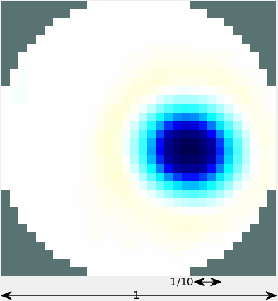
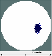
The minimizer of (9) is then obtained using two different approaches: one employs cvx (Figure 3(a)), a package for specifying and solving convex programs [13, 12], the other (Figure 3(b)) uses the MATLAB built-in function quadprog (trust-region-reflective Algorithm). We also show the reconstructed result using the built-in function inv$\_$solve of EIDORS [2] (Figure 3(c)) with the default regularization parameter $0.03$ and with GREIT algorithm [1] (Figure 3(d)) to see that scaling the measured data with the best scaling factor will improve a little bit the reconstructed image. Notice that reconstructed images are highly affected by the choice of the minimization algorithms, and we will see from Figure 3 that the images obtained by cvx has less artifacts than the others.

It is worth to emphasize that although each EIDORS model is assigned to a default regularization parameter, when using the EIDORS built-in function inv$\_$solve [2], in order to obtain a good reconstruction (Figure 2) one has to manually choose a regularization parameter, whilst the regularization parameters ${\it a_{-}}$ and $\beta_{k}$ in our method are known a-priori provided the information of the conductivity $\sigma$ and the reference conductivity $\sigma_{0}$ exists. Besides, if we manually choose the parameters $\min({\it a_{-},\beta_{k}})$, we even get much better reconstructed images (Figure 4).

((a)) $\min(2,\beta_{k})$

((b)) $\min(3,\beta_{k})$

((c)) $\min(4,\beta_{k})$

Figure 4: Reconstructed images for the $9$th-inhomogeneous voltage measurements with monotonicity-based algorithm and different choices of lower constraint.

Table 1: Runtime of pictures in Figure 3

Algorithm	Runtime (second)
cvx	839.3892
quadprog (trust-region-reflective)	5.4467
EIDORS (inv$\_$solve)	0.0231
GREIT	0.0120

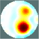
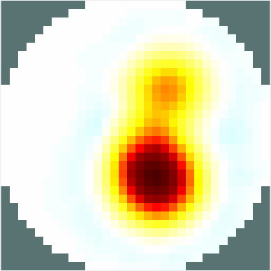
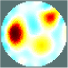
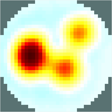
Last but not least, our new method proves its advantage when there are more than one inclusions (Figure 5).

Figure 5: Reconstructed images for simulated data with $0.1\%$ noise. (From left to right) First column: True conductivity change, Second column: our new method (with cvx), Third column: EIDORS (inv$\_$solve), Last column: GREIT

5 Conclusions

In this paper, we have presented a new algorithm to reconstruct images in EIT in the real electrode setting. Numerical results show that this new algorithm helps to reduce the ringing artifacts in the reconstructed images. Global convergence result of this algorithm has been proved in [19] for the Continuum Model. In future works, we shall prove global convergence result for the Shunt Model setting as well as reduce the runtime to fit with real-time applications.

References

- [1] A. Adler, J. H. Arnold, R. Bayford, A. Borsic, B. Brown, P. Dixon, T. J. Faes, I. Frerichs, H. Gagnon, Y. Gärber, et al. GREIT: a unified approach to 2D linear EIT reconstruction of lung images. Physiological measurement, 30(6):S35, 2009.
- [2] A. Adler and R. Guardo. Electrical impedance tomography: regularized imaging and contrast detection. IEEE transactions on medical imaging, 15(2):170–179, 1996.
- [3] A. Adler and W. R. Lionheart. Uses and abuses of eidors: an extensible software base for eit. Physiological measurement, 27(5):S25, 2006.
- [4] R. G. Aykroyd, M. Soleimani, and W. R. Lionheart. Conditional Bayes reconstruction for ERT data using resistance monotonicity information. Measurement Science and Technology, 17(9):2405, 2006.
- [5] M. Azzouz, M. Hanke, C. Oesterlein, and K. Schilcher. The factorization method for electrical impedance tomography data from a new planar device. International Journal of Biomedical Imaging, 2007.
- [6] B. Brown and A. Seagar. The Sheffield data collection system. Clinical Physics and Physiological Measurement, 8(4A):91, 1987.
- [7] M. Cheney, D. Isaacson, J. Newell, S. Simske, and J. Goble. NOSER: An algorithm for solving the inverse conductivity problem. International Journal of Imaging Systems and Technology, 2(2):66–75, 1990.
- [8] K.-S. Cheng, D. Isaacson, J. Newell, and D. G. Gisser. Electrode models for electric current computed tomography. Biomedical Engineering, IEEE Transactions on, 36(9):918–924, 1989.
- [9] M. K. Choi, B. Harrach, and J. K. Seo. Regularizing a linearized eit reconstruction method using a sensitivity-based factorization method. Inverse Problems in Science and Engineering, 22(7):1029–1044, 2014.
- [10] H. Garde and S. Staboulis. Convergence and regularization for monotonicity-based shape reconstruction in electrical impedance tomography. arXiv preprint arXiv:1512.01718, 2015.
- [11] B. Gebauer. Localized potentials in electrical impedance tomography. Inverse Probl. Imaging, 2(2):251–269, 2008.
- [12] M. Grant and S. Boyd. Graph implementations for nonsmooth convex programs. In V. Blondel, S. Boyd, and H. Kimura, editors, Recent Advances in Learning and Control, Lecture Notes in Control and Information Sciences, pages 95–110. Springer-Verlag Limited, 2008.
- [13] M. Grant and S. Boyd. CVX: Matlab software for disciplined convex programming, version 2.1. http://cvxr.com/cvx, Mar. 2014.
- [14] M. Hanke, B. Harrach, and N. Hyvönen. Justification of point electrode models in electrical impedance tomography. Mathematical Models and Methods in Applied Sciences, 21(06):1395–1413, 2011.
- [15] M. Hanke and A. Kirsch. Sampling methods. In O. Scherzer, editor, Handbook of Mathematical Models in Imaging, pages 501–550. Springer, 2011.
- [16] B. Harrach. Recent progress on the factorization method for electrical impedance tomography. Computational and mathematical methods in medicine, 2013.
- [17] B. Harrach. Interpolation of missing electrode data in electrical impedance tomography. Inverse Problems, 31(11):115008, 2015.
- [18] B. Harrach, E. Lee, and M. Ullrich. Combining frequency-difference and ultrasound modulated electrical impedance tomography. Inverse Problems, 31(9):095003, 2015.
- [19] B. Harrach and M. N. Minh. Enhancing residual-based techniques with shape reconstruction features in Electrical Impedance Tomography. arXiv preprint arXiv:1511.07079, 2015.
- [20] B. Harrach and J. K. Seo. Exact shape-reconstruction by one-step linearization in electrical impedance tomography. SIAM Journal on Mathematical Analysis, 42(4):1505–1518, 2010.
- [21] B. Harrach, J. K. Seo, and E. J. Woo. Factorization method and its physical justification in frequency-difference electrical impedance tomography. Medical Imaging, IEEE Transactions on, 29(11):1918–1926, 2010.
- [22] B. Harrach and M. Ullrich. Monotonicity-based shape reconstruction in electrical impedance tomography. SIAM Journal on Mathematical Analysis, 45(6):3382–3403, 2013.
- [23] B. Harrach and M. Ullrich. Resolution guarantees in electrical impedance tomography. IEEE transactions on medical imaging, 34(7):1513–1521, 2015.
- [24] M. Ikehata. Size estimation of inclusion. J. Inverse Ill-Posed Probl., 6(2):127–140, 1998.
- [25] H. Kang, J. K. Seo, and D. Sheen. The inverse conductivity problem with one measurement: stability and estimation of size. SIAM J. Math. Anal., 28(6):1389–1405, 1997.
- [26] T. I. Oh, K. H. Lee, S. M. Kim, H. Koo, E. J. Woo, and D. Holder. Calibration methods for a multi-channel multi-frequency eit system. Physiological measurement, 28(10):1175, 2007.
- [27] T. I. Oh, H. Wi, D. Y. Kim, P. J. Yoo, and E. J. Woo. A fully parallel multi-frequency eit system with flexible electrode configuration: Khu mark2. Physiological measurement, 32(7):835, 2011.
- [28] T. I. Oh, E. J. Woo, and D. Holder. Multi-frequency eit system with radially symmetric architecture: Khu mark1. Physiological measurement, 28(7):S183, 2007.
- [29] T. I. Oh, E. J. Woo, and D. Holder. Multi-frequency EIT system with radially symmetric architecture: KHU Mark1. Physiol. Meas., 28:S183–S196, 2007.
- [30] A. Tamburrino. Monotonicity based imaging methods for elliptic and parabolic inverse problems. Journal of Inverse and Ill-posed Problems, 14(6):633–642, 2006.
- [31] A. Tamburrino and G. Rubinacci. A new non-iterative inversion method for electrical resistance tomography. Inverse Problems, 18(6):1809, 2002.
- [32] H. Wi, H. Sohal, A. L. McEwan, E. J. Woo, and T. I. Oh. Multi-frequency electrical impedance tomography system with automatic self-calibration for long-term monitoring. Biomedical Circuits and Systems, IEEE Transactions on, 8(1):119–128, 2014.
- [33] L. Zhou, B. Harrach, and J. K. Seo. Monotonicity-based electrical impedance tomography lung imaging. preprint, 2015.