Feasibility Based Large Margin Nearest Neighbor Metric Learning

Abstract

Large margin nearest neighbor (LMNN) is a metric learner which optimizes the performance of the popular $k$NN classifier. However, its resulting metric relies on pre-selected target neighbors. In this paper, we address the feasibility of LMNN’s optimization constraints regarding these target points, and introduce a mathematical measure to evaluate the size of the feasible region of the optimization problem. We enhance the optimization framework of LMNN by a weighting scheme which prefers data triplets which yield a larger feasible region. This increases the chances to obtain a good metric as the solution of LMNN’s problem. We evaluate the performance of the resulting feasibility-based LMNN algorithm using synthetic and real datasets. The empirical results show an improved accuracy for different types of datasets in comparison to regular LMNN.

1 Introduction

Metric learning is the idea of finding an efficient metric for a given dataset to provide a more discriminant representation and consequently having a better classification performance. In basic terms, it tries to compact points of the same class while increasing the distance between different classes [2]. A well-known metric learning approach is the Large Margin Nearest Neighbor algorithm (LMNN) [3] which transfers the maximum margin concept of SVM [4] to the $k$-nearest neighbor ($k$NN) framework [5]. LMNN has been used in many real problems such as face recognition [6], motion classification [7] and person identification [8]. Several improvements have been suggested for the original LMNN approach such as complexity reduction of its optimization [9], eigenvalue based optimization [10], multi-tasking extension [11] and hierarchical prepossessing of input data [12]. One challenge of LMNN is the efficient selection of neighboring targets in its optimization framework [3]. As a common strategy, these target points are selected as nearest neighbors from the same class based on the Euclidean distance. In multiple-pass LMNN, the neighborhood is recomputed based on the found distance measure to improve the classification result [3, 13].

In this paper we focus on the relation between selected neighboring targets and the feasible set of LMNN’s optimization problem. We show that wrong choices of targets can severely shrink the regime of feasible solutions of the optimization problem. We introduce a feasibility measure which quantifies the impact of neighboring points with respect to the size of the feasible set, and we use this measure as a weighting scheme in a modified version of LMNN.
Road map: In section 2 we shortly review the original LMNN framework, and afterwards we study the concept of infeasible target neighbors. In section 4 we introduce a measure to evaluate the size of target’s feasible regions, and we introduce feasibility-based LMNN in section 5. We implement our algorithm on synthetic and real datasets in section 6, and eventually the conclusion will be made in the last section.

2 Large Margin Nearest Neighbor Algorithm

Consider the training set $\{(\vec{x}_{i},y_{i})\}_{i=1}^{n}$ with data vectors $\vec{x}_{i}\in\mathbb{R}^{d}$ and their corresponding labels $y_{i}\in\{1,\ldots,C\}$. LMNN tries to find a Mahalanobis metric of the form ${\cal D}_{\mathbf{M}}(\vec{x}_{i},\vec{x}_{j})=(\vec{x}_{i}-\vec{x}_{j})^{\top}\mathbf{M}(\vec{x}_{i}-\vec{x}_{j})$ where $\mathbf{M}$ is a positive semidefinite (psd) matrix. Its objective is to achieve compact neighboring data samples with the same label (targets) and far away neighboring points with different labels (impostors). Define $\mathcal{N}^{k}_{i}$ as the set of points within the $k$-nearest neighbors of $\vec{x}_{i}$ which have the same class and $\mathcal{I}^{k}_{i}$ as the set of points within the $k$-nearest neighbors of $\vec{x}_{i}$ which have a different class. LMNN optimizes the following problem:

$$\begin{array}[]{ll}\underset{\mathbf{M}}{\min}&(1-\mu){\sum}_{i}\sum_{j\in\mathcal{N}^{k}_{i}}{\cal D}_{\mathbf{M}}(\vec{x}_{i},\vec{x}_{j})+\mu\sum_{i}\sum_{j\in\mathcal{N}^{k}_{i}}\sum_{l\in\mathcal{I}^{k}_{i}}\xi_{ijl}\\ \mathrm{s.t.}&{\cal D}_{\mathbf{M}}(\vec{x}_{i},\vec{x}_{l})-{\cal D}_{\mathbf{M}}(\vec{x}_{i},\vec{x}_{j})\geq 1-\xi_{ijl}\\ &\xi_{ijl}\geq 0,~{}~{}{\mathbf{M}}\succeq 0\,~{}~{}\forall i,j\in\mathcal{N}^{k}_{i},l\in\mathcal{I}^{k}_{i}\end{array}$$ (1)

where $\mu\in(0,1)$ balances the two objectives. $\xi_{ijl}$ constitute slack variables of the constraints. Eq.1 constitutes a convex problem with respect to $\mathbf{M}$ if the targets $\mathcal{N}^{k}_{i}$ and impostors $\mathcal{I}^{k}_{i}$ are fixed [3]. Nevertheless, different selections for these initial targets can lead to different solution $\mathbf{M}$. As suggested in [3, 13] a better strategy is to repeat LMNN’s optimization multiple times (multiple-pass LMNN) while updating $\mathcal{N}^{k}_{i}$ and $\mathcal{I}^{k}_{i}$ in each run based on the resulting quadratic form $\mathbf{M}$. Yet, also this strategy relies on the quality of the initial selection of these two sets.

3 Infeasible Target Neighbors

We are interested in the question in which cases feasible solutions of the optimization problem (1) exist which do not require slack variables $\xi_{ijl}>0$. This feasible regime is given as

$$S:=\{\mathbf{M}\in\mathbb{R}^{d\times d}|\mathbf{M}\succeq 0,{\cal D}_{\mathbf{M}}(\vec{x}_{i},\vec{x}_{j})<{\cal D}_{\mathbf{M}}(\vec{x}_{i},\vec{x}_{l})~{}~{}\forall i,j\in\mathcal{N}^{k}_{i},l\in\mathcal{I}^{k}_{i}\}$$ (2)

For a triplet $i$, $j$, $l$, the metric constraint can be re-written as:

$$\begin{array}[]{ll}&\mathrm{Tr}[\mathbf{Q}_{ijl}\mathbf{M}]:=\mathrm{Tr}[((\vec{x}_{i}-\vec{x}_{j})(\vec{x}_{i}-\vec{x}_{j})^{\top}-(\vec{x}_{i}-\vec{x}_{l})(\vec{x}_{i}-\vec{x}_{l})^{\top})\mathbf{M}]<0\\ \end{array}$$ (3)

Since $\mathbf{M}$ is psd, a psd matrix $\mathbf{Q}_{ijl}$ leads to the infeasibility of Eqn. (3), whereby this fact depends on the triplet $i$, $j$, $l$, only, and not the specific neighborhood. In this section, we discuss an extremal case, where the constraint induced by a triplet is infeasible, and we propose an according measure which has a clear geometric interpretation in this extremal case. In the next section, we generalize this measure to a suitable weighting scheme for more general settings.

A matrix $\mathbf{Q}:=\mathbf{Q}_{ijl}$ results from two vectors in the form $\vec{a}\vec{a}^{\top}-\vec{b}\vec{b}^{\top}$, i.e. its rank is at most $2$. After matrix transformation if necessary, we can assume that only the first two dimensions of the matrix, $\vec{a}$ and $\vec{b}$ relate to non-zero coefficients. Denote the two possibly nonzero eigenvalues of $\mathbf{Q}$ as $\lambda_{\mathrm{min}}(\mathbf{Q})\leq\lambda_{\mathrm{max}}(\mathbf{Q})$. Note that eigenvectors are obviously located in the span of $\vec{a}$ and ${\vec{b}}$, and (after base transformation s.t. non-zero coefficients are denoted $(a_{1},a_{2})$ and $(b_{1},b_{2})$) they have the form

$$\lambda_{\mathrm{max}/\mathrm{min}}=(a_{1}^{2}+a_{2}^{2}-b_{1}^{2}-b_{2}^{2})/2\pm\sqrt{(a_{1}^{2}+a_{2}^{2}-b_{1}^{2}-b_{2}^{2})^{2}/4+(a_{1}b_{2}-b_{1}a_{2})^{2}}$$

as one can easily infer from the characteristic polynomial of $\mathbf{Q}$. Obviously, $\lambda_{\mathrm{min}}(\mathbf{Q})\leq 0<\lambda_{\mathrm{max}}(\mathbf{Q})$ (unless vectors itself are degenerate). The equality $\lambda_{\mathrm{min}}(\mathbf{Q})=0$ corresponds to linearly dependent vectors $\vec{a}$ and $\vec{b}$, namely the equality $a_{1}b_{2}-b_{1}a_{2}=0$. This setting does not allow a feasible solution without slack variables. In the following, we will argue that the measure $r:=-\lambda_{\mathrm{min}}(\mathbf{Q})/\lambda_{\mathrm{max}}(\mathbf{Q})$ constitutes a reasonable weight vector to measure the feasibility of the constraint corresponding to $\mathbf{Q}$ or the size of its feasible domain, respectively. Obviously, $r=0$ is the case just described, an infeasible setting due to the geometry of $\vec{a}=(\vec{x}_{i}-\vec{x}_{j})$ and $\vec{b}=(\vec{x}_{i}-\vec{x}_{l})$.

4 Feasibility Measure

We start with a general observation:

Lemma 1.

Denote the eigenvalues of a matrix $\mathbf{Q}\in\mathrm{R}^{d\times d}$ by $\lambda_{1}(\mathbf{Q})\geq\lambda_{2}(\mathbf{Q})\geq\ldots$. The smallest/largest eigenvalue is denoted $\lambda_{min}({\mathbf{Q}})$ resp. $\lambda_{max}({\mathbf{Q}})$. For hermitian $\mathbf{Q}\in\mathrm{R}^{d\times d}$ and symmetric psd $\mathbf{M}\in\mathrm{R}^{d\times d}$, it holds $\lambda_{k}({\mathbf{Q}})\lambda_{min}({\mathbf{M}})\leq\lambda_{k}({\mathbf{QM}})$ for all $k$.

Proof.

$\mathbf{M}$ is psd and $\mathbf{Q}$ and $\mathbf{M}$ are symmetric, hence $\lambda_{k}({\mathbf{QM}})=\lambda_{k}({\mathbf{Q}\sqrt{\mathbf{M}}\sqrt{\mathbf{M}}})=\lambda_{k}({\sqrt{\mathbf{M}}\mathbf{Q}\sqrt{\mathbf{M}}})$ where $\sqrt{\mathbf{M}}$ is the principal square root of $\mathbf{M}$. Using the min-max theorem we find $\lambda_{k}({\mathbf{QM}})=\underset{{\dim(F)=k}}{\mathrm{min}}\left(\max_{x\in F\backslash\{0\}}\frac{\langle Q\sqrt{\mathbf{M}}x,\sqrt{\mathbf{M}}x\rangle}{\langle\sqrt{\mathbf{M}}x,\sqrt{\mathbf{M}}x\rangle}\frac{\langle\mathbf{M}x,x\rangle}{{\langle x,x\rangle}}\right)\geq\lambda_{min}({\mathbf{M}})\,\underset{\dim(F)=k}{\mathrm{min}}\left(\max_{x\in F\backslash\{0\}}\frac{\langle\mathbf{Q}\sqrt{\mathbf{M}}x,\sqrt{\mathbf{M}}x\rangle}{\langle\sqrt{\mathbf{M}}x,\sqrt{\mathbf{M}}x\rangle}\right)$ because $\frac{\langle\mathbf{M}x,x\rangle}{\langle x,x\rangle}\geq\lambda_{min}(\mathbf{M})$.
Again using the min-max theorem we get $\lambda_{k}({\mathbf{QM}})\geq\lambda_{min}({\mathbf{M}})\lambda_{k}({\mathbf{Q}})$. ∎

Based on Lemma 1 we have $\lambda_{max}({\mathbf{Q}})\lambda_{min}({\mathbf{M}})\leq\lambda_{max}({\mathbf{QM}})$ for $\mathbf{Q}:=\mathbf{Q}_{ijl}$ as specified above. In the setting $\lambda_{min}({\mathbf{Q}})<0<\lambda_{max}({\mathbf{Q}})$, we can use [14](corollary 10) to infer $\lambda_{min}({\mathbf{Q}})\lambda_{max}({\mathbf{M}})\leq\lambda_{min}({\mathbf{QM}})$. Combining these two inequalities results in the inequality

$$\lambda_{min}({\mathbf{Q}})\lambda_{max}({\mathbf{M}})+\lambda_{max}({\mathbf{Q}})\lambda_{min}({\mathbf{M}})\leq\mathrm{Tr}(\mathbf{QM})$$ (4)

Eq. 3 induces the objective $\mathrm{Tr}(\mathbf{QM})<0$, hence the left hand side of Eq. 4 should be negative, i.e.  $-\frac{\lambda_{min}({\mathbf{Q}})}{\lambda_{max}({\mathbf{Q}})}>\frac{\lambda_{min}({\mathbf{M}})}{\lambda_{max}({\mathbf{M}})}$. Hence a triplet $i,j,l$ with a small value $r=-\frac{\lambda_{min}({\mathbf{Q}})}{\lambda_{max}({\mathbf{Q}})}$ imposes a tight constraint on the eigenvalue formation of $\mathbf{M}$, hence we expect an induced small feasible set $S_{ijl}$. Note that the feasible domain $S$ results as intersection of the feasible sets $S_{ijl}$. We include this observation and the according measure $r=r_{ijl}$ into the optimization framework in the form of an according weighting.

5 Feasibility Based LMNN

For a vector $\vec{x}_{i}$ and a given target $\vec{x}_{j}\in\mathcal{N}^{k}_{i}$ we define $R_{ij}:=\underset{\vec{x}_{l}\in\mathcal{I}^{k}_{i}}{\min}(r_{ijl})$. We formulate feasibility-based LMNN as the following LMNN problem which incorporates according weights of the objective:

$$\begin{array}[]{ll}\underset{\mathbf{M}}{\min}&(1-\mu){\sum}_{i}\sum_{j\in\mathcal{N}^{k}_{i}}R_{ij}{\cal D}_{\mathbf{M}}(\vec{x}_{i},\vec{x}_{j})+\mu\sum_{i}\sum_{j\in\mathcal{N}^{k}_{i}}R_{ij}\sum_{l\in\mathcal{I}^{k}_{i}}\xi_{ijl}\\ \mathrm{s.t.}&{\cal D}_{\mathbf{M}}(\vec{x}_{i},\vec{x}_{l})-{\cal D}_{\mathbf{M}}(\vec{x}_{i},\vec{x}_{j})\geq 1-\xi_{ijl}\\ &\xi_{ijl}\geq 0,~{}~{}{\mathbf{M}}\succeq 0,~{}~{}\forall i,j\in\mathcal{N}^{k}_{i},l\in\mathcal{I}^{k}_{i}\end{array}$$ (5)

Unlike original LMNN, infeasible or challenging triplets carry less weighting in this formulation. We dub the resulting method FB-LMNN. FB-LMNN is implemented by first determining the neighborhood, computing corresponding weights $R_{ij}$, and then solving the convex optimization problem w.r.t. matrix $\mathbf{M}$. In addition, a multiple passes strategy can be used to increase the resulting accuracy [3].

6 Experiments

We evaluate our algorithm on both synthetic and real data, and compare it with $k$NN, single-path LMNN (SP-LMNN), multiple passes LMNN (MP-LMNN)[3] and multi-class SVM [4]. For LMNN we use a neighborhood size $k=5$ and weighting $\mu=0.5$. Evaluation is done in a 10-fold cross validation. SVM uses the respective best result obtained with a linear, RBF-, or polynomial kernel.

6.1 Synthetic Data

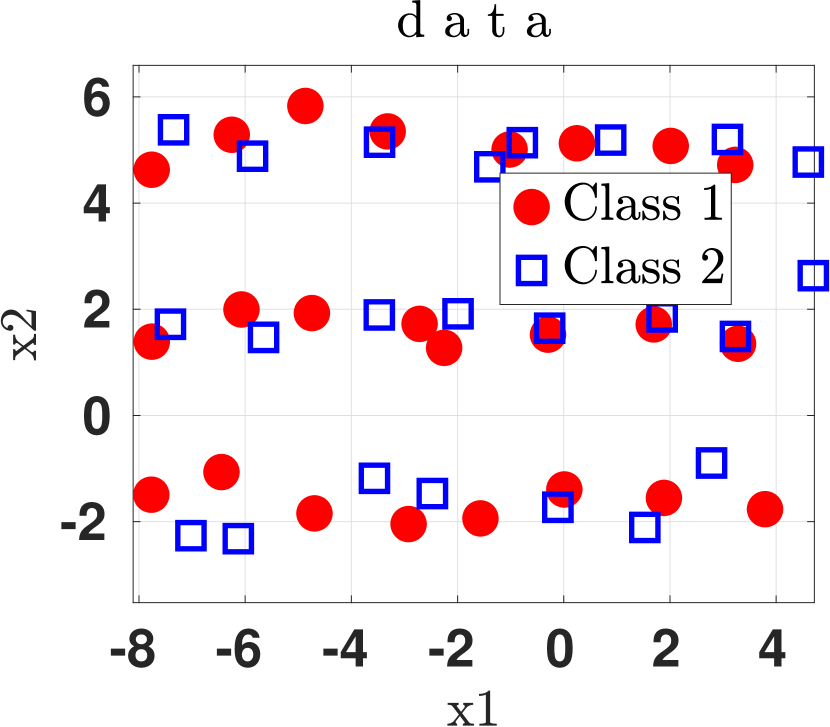
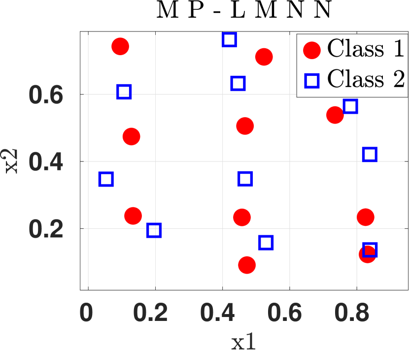
The synthetic dataset is a variation of the 2D zebra stripe data from [3] in which two classes of data alternate (Fig.1-left). In contrast to [3], the nearest targets to each data point $\vec{x}_{i}$ are located on the same stripe. On each stripe, the impostors and targets are almost placed on a straight line, resulting in very tight or infeasible constraints of the optimization framework. Even multiple-pass LMNN (Fig.1-middle) does hardly change this selection of impostors and targets. Consequently multiple-pass LMNN converges to a non-optimal solution $\mathbf{M}$ with classification accuracy of $23.51\%$ (almost the same as $k$NN’s).

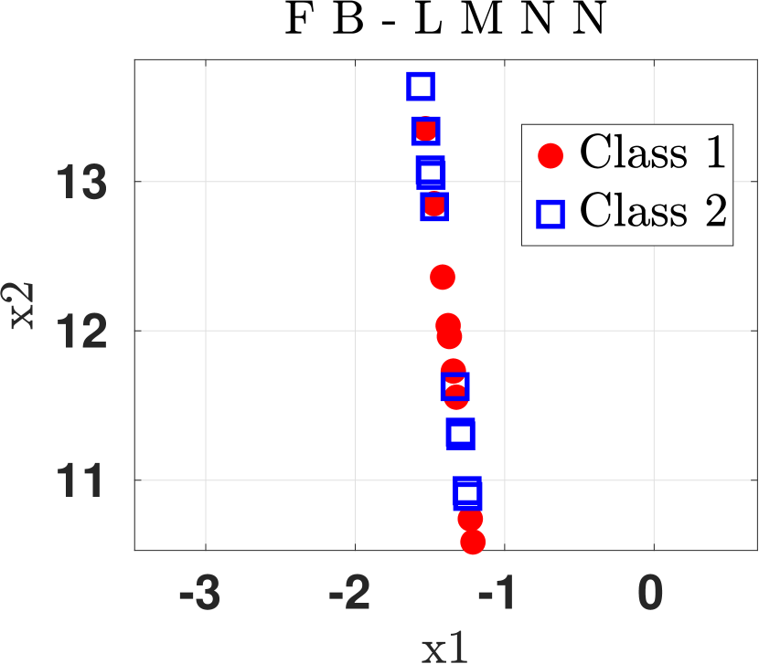
On the other hand, FB-LMNN assigns small $R_{ij}$ weights to pairs within the same stripe while bigger weights to pairs in neighbored stripes. Therefore it obtains a different matrix $\mathbf{M}$ which results in a different scaling of the space (Fig.1-right), and a classification accuracy of $72.21\%$.

Figure 1: Zebra dataset (top-left), MP-LMNN (top-right) and FB-LMNN (bottom)

6.2 Real Datasets

Real datasets are mostly taken from the UCI repository library; in addition, we consider the extended Yale face dataset and the MNIST handwritten digits, which constitute benchmarks in this domain. The selected datasets cover different application areas and types of the data set. For the Yale face, MNIST, and isolet datasets we follow the procedure proposed in [3] as regards preprocessing by means of dimensionality reduction and the cross-validation procedure for evaluation.

Results are shown in Table 1. FB-LMNN significantly surpasses MP-LMNN in some cases, demonstrating the effectivity of the proposed feasibility measure $R$. For a few data sets, such as the Yale dataset, no significant difference is observed. Interestingly, results as obtained by SVM are mostly on par, but in some cases worse as compared to FB-LMNN, whereby SVM restricts to the standard Euclidean metric. It would be an interesting endeavor to test the effect of the metric learned by FB–LMNN on the result of SVM.

Table 1: Classification accuracy(%) and datasets’ characteristics.

dataset	class	dimension	$k$NN	sp-lmnn	mp-lmnn	fb-lmnn	SVM
Zebra	2	2	21.31	22.41	23.51	72.21	50.82
Wine	3	13	76.20	92.84	93.91	98.77	78.23
Balance	3	4	83.42	88.45	94.03	96.08	97.5
B. Cancer	20	30	94.66	94.88	96.68	97.07	78.49
Car Eval.	4	6	92.57	95.12	98.32	98.4	60.08
Tic-Tac-Toe	2	9	87.42	91.46	97.66	98.13	85
Hepatitis	2	17	84.16	84.46	84.46	90	79.11
iris	3	4	94.93	95.02	95.61	96.05	96.13
isolet	26	172	91.02	95.64	95.70	96.85	96.60
YFace	38	300	89.21	94.10	94.48	94.48	84.78
MNIST	10	164	97.57	98.28	98.31	98.92	98.80

7 Conclusion

In this paper we studied the role of target neighbors $\mathcal{N}^{k}_{i}$ on the feasibility of the constraints in LMNN’s optimization problem. We proposed a quantitative measure for the degree of feasibility of triplets of a target and impostor for a data point, and we demonstrated that this measure constitutes an efficient and effective weighting scheme to be integrated into LMNN’s optimization. The results of several experiments clearly demonstrate the effect of the proposed technology.

References

- [1] Babak Hosseini and Barbara Hammer. Feasibility based large margin nearest neighbor metric learning. In ESANN 2018-26th European Symposium on Artificial Neural Networks, 2018.
- [2] Aurélien Bellet, Amaury Habrard, and Marc Sebban. A survey on metric learning for feature vectors and structured data. arXiv preprint arXiv:1306.6709, 2013.
- [3] Kilian Q. Weinberger and Lawrence K. Saul. Distance metric learning for large margin nearest neighbor classification. Journal of Machine Learning Research, 10:207–244, 2009.
- [4] Koby Crammer and Yoram Singer. On the algorithmic implementation of multiclass kernel-based vector machines. Journal of machine learning research, 2(Dec):265–292, 2001.
- [5] Thomas Cover and Peter Hart. Nearest neighbor pattern classification. IEEE transactions on information theory, 13(1):21–27, 1967.
- [6] Matthieu Guillaumin, Jakob Verbeek, and Cordelia Schmid. Is that you? metric learning approaches for face identification. In 2009 IEEE 12th International Conference on Computer Vision, pages 498–505. IEEE, 2009.
- [7] B. Hosseini and B. Hammer. Efficient metric learning for the analysis of motion data. In IEEE International Conference on Data Science and Advanced Analytics (DSAA), 2015., pages 1–10, Oct 2015.
- [8] Penglin Li, Mengxue Liu, Yun Gu, Lixiu Yao, and Jie Yang. Adaptive multi-metric fusion for person re-identification. In CCPR2016, pages 258–267. Springer, 2016.
- [9] Kyoungup Park, Chunhua Shen, Zhihui Hao, Junae Kim, et al. Efficiently learning a distance metric for large margin nearest neighbor classification. In AAAI, 2011.
- [10] Yiming Ying and Peng Li. Distance metric learning with eigenvalue optimization. Journal of Machine Learning Research, 13(Jan):1–26, 2012.
- [11] Shibin Parameswaran and Kilian Q Weinberger. Large margin multi-task metric learning. In Advances in neural information processing systems, pages 1867–1875, 2010.
- [12] Heng Zhang, Vishal M Patel, and Rama Chellappa. Hierarchical multimodal metric learning for multimodal classification. In CVPR2017, pages 3057–3065, 2017.
- [13] Christina Göpfert, Benjamin Paassen, and Barbara Hammer. Convergence of multi-pass large margin nearest neighbor metric learning. In International Conference on Artificial Neural Networks, pages 510–517. Springer, 2016.
- [14] Fuzhen Zhang, Qingling Zhang, et al. Eigenvalue inequalities for matrix product. IEEE Transactions on Automatic Control, 51(9):1506, 2006.