Electromagnetic shift arising from the Heisenberg-Euler dipole

Abstract

We show that photons may be redshifted or blueshifted when interacting with the field of an overcritical dipole, which incorporates the one-loop QED corrections coming from vacuum polarization. Using the effective metric, it follows that such effect depends on the polarization of the photon. The shifts, plotted against the azimuthal angle for various values of the magnetic field, may show an intensity comparable to the gravitational redshift for a magnetar. To obtain these results, we have corrected previous literature.

1 Introduction

Nonlinear electromagnetic (EM) theories have been widely studied both in the classical and quantum realm. Born and Infeld’s theory [1], in which the field of a charged particle is regular everywhere, is an example of the former type. Still on the classical side, the effect of gravity has been analyzed in several papers, including black holes sourced by a nonlinear EM field [2]. The latter type is based on the nonlinear corrections that Maxwell’s Lagrangian gains due to vacuum polarization, as shown by Heisenberg and Euler (HE)[3]. The corrections are important when the fields reach a value comparable to the critical electric $E_{c}\approx 1.3\times 10^{18}$ V/m or magnetic $B_{c}\approx 4.4\times 10^{13}$ G field. There are several testable predictions that follow from the Heisenberg-Euler Lagrangian: the Schwinger effect [4] ,the birefringence of the vacuum under a strong magnetic field [5], currently under experimental observation [6, 7], and photon splitting [8] in a laser field [9].

Beyond the experimental effort on earth, some compact astrophysical objects may offer the possibility of testing the quantum vacuum. The magnetars are neutron stars endowed with an overcritical magnetic field [10], with estimated values up to $10^{2}B_{c}$ at their surface [11]. Several consequences of such intense field have been studied: such as the lensing of the light emitted by background astronomical objects due to the optical properties of quantum vacuum in the presence of a magnetic field [12], the polarization phase lags due to the index of refraction of the vacuum [13], and the influence of the quantum vacuum friction on the spindown of pulsars [14].

Many of these effects are related to photon propagation in a background field, which can be studied using the effective metric. The propagation of the high energy excitations of a nonlinear EM theory on a fixed background is governed by an effective metric [15, 16] that depends on the background spacetime metric, on the background EM field configuration, and on the details of the nonlinear dynamics obeyed by the EM field [17]. There are numerous applications of the effective metric in pure gravity [16] , and cosmology [18]. In an astrophysical setting, it was shown for the case of BI’s theory [19] and for the low-field correction to Maxwell’s Lagrangian obtained from HE’s Lagrangian [20] that high energy photons coming from a compact object endowed with an overcritical field would display an EM redshift, in addition to the gravitational redshift. The EM redshift (or blueshift, as we shall see below) is rooted in the nonlinearities of the Lagrangian, hence it is absent in Maxwell’s theory. Here we investigate the electromagnetic shift (EMS) of photons in a dipole field which is a solution of the full QED one-loop corrected Lagrangian, in a flat space-time background [21], through the effective metric.

2 Effective metric

How the propagation of high energy perturbations on a fixed background of a nonlinear theory with more that one degree of freedom may display birefringence and/or bimetricity was originally discussed [15, 16, 17] for the EM field. A general Lagrangian ${\cal L}$ for a nonlinear EM field can be an arbitrary function of the invariants $F$ and $G$, given by $F=\frac{1}{4}F_{\mu\nu}F^{\mu\nu}$, and $G=\frac{1}{4}^{*}F_{\mu\nu}F^{\mu\nu}$, where ${}^{*}F_{\mu\nu}=\frac{1}{2}\epsilon^{\mu\nu\lambda\sigma}F_{\lambda\sigma}$. The equations of motion following from such a Lagrangian in a flat background are [16]

$$\left[\sqrt{-\eta}\left({\cal L}_{F}F^{\mu\nu}+{\cal L}_{{}^{*}F}\;\;^{*}F^{\mu\nu}\right)\right]_{;\nu}=0,$$ (1)

where $\eta$ is the determinant of the background metric $\eta_{\mu\nu}$; the covariant derivative is constructed with $\eta_{\mu\nu}$, and ${\cal L}_{X}\equiv\partial{\cal L}/\partial X$ [16]. The fields also have to obey the identity $F_{[\mu\nu,\lambda]}=0$. By perturbing the equation of motion with respect to a fixed background EM field, keeping only terms linear in the perturbation, and applying the eikonal approximation [22]), it follows that in the high energy limit the propagation of each of the two polarizations of the EM field is governed by an effective metric, given by

$${}^{(1)}\widetilde{g}^{\mu\nu}=\left[{\cal L}_{F}\,\eta^{\mu\nu}-4\,{\cal L}_{FF}\,{F^{\mu}}_{\alpha}\,F^{\alpha\nu}\right]_{0},$$ (2)

$${}^{(2)}\widetilde{g}^{\mu\nu}=\left[\left({\cal L}_{F}-2F{\cal L}_{GG}\right)\,\eta^{\mu\nu}-4\,{\cal L}_{GG}\,{F^{\mu}}_{\alpha}\,F^{\alpha\nu}\right]_{0},$$ (3)

where the subscript zero means that all the quantities in both effective metrics are evaluated at the background field.

$$1+z=\frac{(\widetilde{g}^{00})^{-1}(E)}{(\widetilde{g}^{00})^{-1}(R)}.$$

The shift can be computed using the usual general relativity formulas, keeping into account that the photons, in these theories, are accelerated by the nonlinearities and therefore, do not move along the geodesics of the background metric[15, 16]. Hence one has

$${}^{(1)}z={\cal L}_{F}(r_{E})-1,$$ (4)

and

$${}^{(2)}z=\left[{\cal L}_{F}(r_{E})-2F(r_{E}){\cal L}_{GG}(r_{E})\right]-1.$$ (5)

where the index $E$ ($R$) refers to the emission (reception) point. In both expressions, the reception point was taken at an infinite distance from $E$, where the effective metric reduces to that of Minkowski.

These expressions are valid for any nonlinear EM theory. In the next section, we shall work with the HE Lagrangian.

3 Heisenberg-Euler Lagrangian

The Heisenber-Euler Lagrangian is an effective Lagrangian for the one-loop QED. Its form is given in Lundin’s paper [23] Eq. (1). This Lagrangian is valid in the so-called soft photon approximation ($\omega\ll$ m). [23] In case of a zero electric field, $F=B^{2}/2$, $G=0$. It is worth pointing out that although the HE Lagrangian was originally derived under the assumption of a constant electric or magnetic field, it can still be used in situations in which the fields are inhomogeneous, through a derivative expansion [24]. In this case, the lowest-order approximation is given by the HE Lagrangian evaluated at the inhomogeneous field. As seen from Eqns. (4) and (5), the dependence of ${\cal L}_{F}$ and ${\cal L}_{GG}$ with the field is needed to calculate the EMS. In terms of $\xi=B/B_{c}$, such functions are given [23] (see Eq. 3a-3c).

4 Calculation of the electromagnetic shift

To compute the EMS associated to each polarization, we use as the background solution that of a dipole oriented along the $z$ axis, namely

$$\phi_{0}({\bf r})=\sqrt{\frac{4\pi}{3}}\frac{d}{r^{2}}Y_{10}(\theta,\phi),$$ (6)

where the background field is calculated from the potential using $\mathbf{B_{0}}=-\boldsymbol{\nabla}\phi_{0}$, and $d$ is the dipolar moment. Since the relevant expressions in both effective metrics are already $O(\alpha)$, only the zero-order solution for the field is needed to calculate the EMS Fig. 1 presents the dependence of the EMS with the variable $\xi$ for both polarizations.

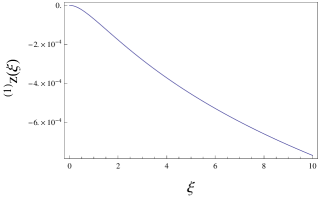
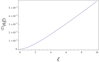
Figure 1: The figure on the left displays the dependence of ${}^{(1)}z$ with $\xi$, while in that on the right, the dependence of ${}^{(2)}z$ with $\xi$ is shown.

The figures show that the EMS is small in both cases as expected from an effect arising from a quantum correction. It is important to remark that the EMS is negative for the first polarization (hence a redshift) and positive (so it is actually a blueshift) and larger for the second.

With the introduction of the parameter $\lambda$, given by the quotient of the mean dipole background field at $r=r_{E}$ and the critical field,

$$\lambda=\frac{d}{r_{E}^{3}B_{c}},$$

it follows that

$$\xi=\frac{B_{0}}{B_{c}}=\lambda(1+3\cos^{2}\theta).$$

Hence, the EMS given by Eqns. (4) and (5) is a function of $\theta$ for each value of $\lambda$. Fig. 2 shows the dependence with $\cos\theta$ of the EMS for three values of $\lambda$, which are relevant for magnetars [10]).

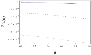
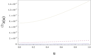
Figure 2: Plot of ${}^{(1)}z$ (left) and ${}^{(2)}z$ in terms of $u=\cos\theta$, for $\lambda=1,10,100$ (continuous, dashed, and dotted line respectively). In the plot on the left, the EMS is negative and decreases with the field. The opposite happens in the plot on the right.

The plots show that in both cases the EMS increases (in absolute value) with the field, but while ${}^{(1)}z$ is maximum at the equator and minimum at the poles, ${}^{(2)}z$ behaves in the opposite way. It also follows from the plots that the EMS is typically one order of magnitude larger for the second polarization.

5 Conclusions

We have derived and computed the EMS that photons experience when emitted at a given point of a dipole field with QED one-loop corrections and travel to infinity. The EMS evidences a polarization dependent effect. The energy exchange between photons and the background field is due to their interaction through the nonlinearities of the theory (since the EMS is null when $\alpha=0$).

This new effect may be important at least in two different areas. In the astrophysics of magnetars, gravitation and rotation should not be neglected, but the significance of the EMS can be seen in a simpler setting, taking into account that the EMS adds to the gravitational redshift [19]. For a star of two solar masses and a radius of $10$ km (typical values for a magnetar), the gravitational redshift (calculated using the Schwarzschild-Droste metric, see Ref.  ro02) would be approximately 0.2. Hence, as shown in Figure 2, for strong enough background fields, the EMS can reach values that are of the order of the gravitational redshift (for one of the polarizations). This effect would lead to a variation in the shift of photons coming from the surface of the star and hence in the ratio of the mass and the radius. Our results may be relevant also in experimental settings to detect the signature of the QED vacuum, in particular those that use an overcritical dipole magnetic field, such as PVLAS and BMV [6, 7]. We hope to report on these developments in future publications.

References

- [1] M. Born and L. Infeld, “Foundations of the new field theory,” Proc. R. Soc. Lond. A, vol. 144, p. 425, 1934.
- [2] N. Bretón and S. E. Perez Bergliaffa, “On the stability of black holes with nonlinear electromagnetic fields,” Ann. Phys., vol. 354, p. 440, 2015.
- [3] W. Heisenberg and H. Euler, “Folgerungen aus der Diracschen theorie des positron,” Z. Phys., vol. 98, p. 714, 1936.
- [4] J. S. Schwinger, “On gauge invariance and vacuum polarization,” Phys. Rev., vol. 82, p. 224, 1951.
- [5] Z. Bialynicka-Birula and I. Bialynicki-Birula, “Nonlinear effects in quantum electrodynamics. Photon propagation and photon splitting in an external field,” Phys. Rev. D, vol. 2, p. 2341, 1970.
- [6] G. Zavattini, F. Della Valle, U. Gastaldi, E. Milotti, G. Messineo, R. Pengo, L. Piemontese, and G. Ruoso, “The PVLAS experiment for measuring the magnetic birefringence of vacuum,” N. Cim. C, vol. 36, p. 41, 2013.
- [7] P. Berceau, M. Fouché, R. Battesti, and C. Rizzo, “Magnetic linear birefringence measurements using pulsed fields,” Phys. Rev. A, vol. 85, p. 013837, 2012.
- [8] S. L. Adler, J. N. Bahcall, C. G. Callan, and M. N. Rosenbluth, “Photon splitting in a strong magnetic field,” Phys. Rev. Lett., vol. 25, p. 1061, 1970.
- [9] A. D. Piazza, A. Milstein, and C. Keitel, “Photon splitting in a laser field,” Phys. Rev. A, vol. 76, p. 032103, 2007.
- [10] S. Mereghetti, “The strongest cosmic magnets: soft gamma-ray repeaters and anomalous x-ray pulsars,” Astron. Astrophys. Rev., vol. 15, p. 225, 2008.
- [11] S. Mereghetti, “Pulsars and magnetars,” Braz. J. Phys., vol. 43, p. 356, 2013.
- [12] A. Dupays, C. Robilliard, C. Rizzo, and G. Bignami, “Observing quantum vacuum lensing in a neutron star binary system,” Phys. Rev. Lett., vol. 96, p. 161101, 2005.
- [13] J. S. Heyl and N. J. Shaviv, “Polarization evolution in strong magnetic fields,” Mon. Not. R. Astr. Soc., vol. 311, p. 555, 2000.
- [14] A. Dupays, C. Rizzo, and G. Bignami, “Quantum vacuum influence on pulsars spindown evolution,” Europhys. Lett., vol. 98, p. 49001, 2012.
- [15] S. Alarcón Gutiérrez, A. L. Dudley, and J. F. Plebañski, “Signals and discontinuities in general relativistic nonlinear electrodynamics,” J. Math. Phys., vol. 22, p. 2835, 1981.
- [16] M. Novello, S. Perez Bergliaffa, and J. Salim, “Singularities in general relativity coupled to nonlinear electrodynamics,” Class. Q. Grav., vol. 17, p. 3821, 2000.
- [17] C. Barceló, S. Liberati, and M. Visser, “Analogue gravity,” Liv. Rev. Rel., vol. 14, no. 3, 2005.
- [18] M. Novello, E. Goulart, J. Salim, and S. Perez Bergliaffa, “Cosmological effects of nonlinear electrodynamics,” Class. Q. Grav., vol. 24, p. 3021, 2007.
- [19] H. J. Mosquera Cuesta and J. M. Salim, “Non-linear electrodynamics and the gravitational redshift of highly magnetized neutron stars,” Mon. Not. R. Astron. Soc., vol. 354, p. L55, 2004.
- [20] H. J. Mosquera Cuesta and J. M. Salim, “Nonlinear electrodynamics and the surface redshift of pulsars,” Astrophys. J., vol. 608, p. 925, 2004.
- [21] J. S. Heyl and L. Hernquist, “QED one-loop corrections to a macroscopic magnetic dipole,” J. Phys. A Math. Gen., vol. 30, p. 6475, 1997.
- [22] M. Visser, C. Barceló, and S. Liberati, “Birefringence versus bimetricity,” in Inquiring the universe: essays to celebrate Professor Mario Novello’s Jubilee, J. M. Salim, S. E. Perez Bergliaffa, L. A. Oliveira, and V.A. De Lorenci, eds., p. 397 (Paris, Frontier Group, 2003).
- [23] J. Lundin, “An effective action approach to photon propagation on a magnetized background,” Europhys. Lett., vol. 87, p. 31001, 2009.
- [24] G. V. Dunne, “Heisenberg-Euler effective Lagrangians: basics and extensions,” in From fields to strings: circumnavigating theoretical physics, Ian Kogan memorial collection (M. Shifman, A. Vainshtein, and J. Wheater, eds.), vol. 1, p. 445 (Singapore, World Scientific, 2004).
- [25] T. Rothman, “Editor’s note: the field of a single centre in Einstein’s theory of gravitation, and the motion of a particle in that field,” Gen. Rel. Grav., vol. 34, p. 1541, 2002.