Dynamics of Particles around Time Conformal Schwarzschild Black Hole

Abstract

In this work, we present the new technique for discussing the dynamical motion of neutral as well as charged particles in the absence/presence of magnetic field around the time conformal Schwarzschild black hole. Initially, we find the numerical solutions of geodesics of Schwarzschild black hole and the time conformal Schwarzschild black hole. We observe that the Schwarzschild spacetime admits the time conformal factor $e^{\epsilon f(t)}$, where $f(t)$ is an arbitrary function and $\epsilon$ is very small which causes the perturbation in the spacetimes. This technique also re-scale the energy content of spacetime. We also investigate the thermal stability, horizons and energy conditions corresponding time conformal Schwarzschild spacetime. Also, we examine the dynamics of neutral and charged particle around time conformal Schwarzschild black hole. We investigate the circumstances under which the particle can escape from vicinity of black hole after collision with another particle. We analyze the effective potential and effective force of particle in the presence of magnetic field with angular momentum graphically.

1 Introduction

The dynamics of particles (massless or massive, neutral or charged) in the vicinity of black hole (BH) is the most intriguing problems in the BH astrophysics. The geometrical structure of spacetime in the surrounding of BH could be studied better by these phenomenon [1, 2]. The motion of particles help us to understand gravitational fields of BHs experimentally and to compare them with observational data. The magnetic field in the vicinity of BH is due to the presence of plasma [3]. Magnetic fields can’t change the geometry of BH but its interaction with plasma and charged particles is very important [4, 5]. The transfer of energy to particles moving around BH geometry is due to magnetic field, so that there is a possibility of their escape to spatial infinity [6]. Hence, the high energy may produce by charged particles collision in the presence of magnetic field rather than its absence.

Recent observations have also provided hints about connecting magnetars with very massive progenitor stars, for example an infrared elliptical ring or shell was discovered surrounding the magnetar SGR $1900+14$ [7]. The explanation of magnetic white dwarfs was first proposed in the scenario of fossil-field for magnetism of compact objects [8, 9, 10]. Magnetic white dwarfs may be created as a result of rebound shock explosion [10] and may further give rise to novel magnetic modes of global stellar oscillations [11]. This fossil-field scenario is supported by the statistics for the mass and magnetic field distributions of magnetic white dwarfs. Magnetized massive progenitor stars with a quasi-spherical general polytropic magneto fluid under the self-gravity are modeled by [12]. Over recent years methods are being developed to detect truly cosmologically magnetic fields, not associated with any virilized structure. The spectral energy distribution of some tera electron-volt range (TeV) blazers in the TeV and giga electron volt (GeV) range hint at the presence of a cosmological magnetic field pervading all space [13, 14].

Authors [15, 16, 17] investigated effects on charged particles in the presence of magnetic field near BHs. The motion of charged particles discussed by Jamil et al. [18] around weakly magnetized BHs in JNW space time. Many aspects of motion of particles around Schwarzschild and Reissner-Nordstrom BH have been studied and the detail review is given the reference [19, 20]. An important question may rise in the studies of these important problems is ”what will happen in the dynamics of particles (neutral or charged) around BHs with respect to time”. Particles moves in circular orbits around BHs in equatorial plane may show drastic change with respect to time. Following the work done by Zaharani et al. [20], we present at what conditions particle escape to infinity after collision. At some specific time interval, we study the dynamics of neutral and charged particles around time conformal Schwarzschild BH.

The purpose of our work is to investigate under which circumstances the particle moving initially would escape from innermost stable circular orbit (ISCO) or it remain bounded, captured by BH or escape to infinity after collision with another particle. We calculate the escape velocity of particle and investigate some important characteristics such as effective potential and effective force of particle motions around the BH with respect to time. Initially, we will find attraction in particle motion but after some specific time we see the repulsion. The comparison of stability orbits of particle with the help of Lyapunov exponent is also established.

The outline of paper is as follows: In section 2, we discuss the Noether and Approximate Noether Symmetries for Schwarzschild BH and time conformal Schwarzschild BH and find the corresponding conservation laws. In section 3, we investigate the dynamics of neutral particle through effective potential, effective force and escape velocity. In section 4, the motion of charged particle is discussed, the behavior of effective potential, effective force and escape velocity is analyzed in the presence of magnetic field. In section 5, the Lyapunov exponent is discussed. Conclusion and observations are given in the last section.

2 Noether and Approximate Noether Symmetries and Corresponding Conservation Laws

The one to one correspondence between conservation laws and symmetries of Lagrangian (Noether symmetries) has been firstly pointed out by Emmy Noether [21, 22, 23]. She suggested that there exist a conservation law for every Noether symmetry. One can obtain the approximate Noether symmetries of Schwarzschild solution by considering its first order perturbation and investigate the energy-momentum of corresponding spacetime.

2.1 Schwarzschild Black Hole

The line element of the Schwarzschild solution is

$$ds^{2}_{e}=(1-\frac{2M}{r})dt^{2}-(1-\frac{2M}{r})^{-1}dr^{2}-r^{2}({d\theta}^{2}+\sin\theta{d\phi}^{2}).$$ (1)

the corresponding Lagrangian is

$$L_{e}=(1-\frac{2M}{r})\dot{t}^{2}-(1-\frac{2M}{r})^{-1}\dot{r}^{2}-r^{2}(\dot{\theta}^{2}+\sin\theta\dot{\phi}^{2}).$$ (2)

The symmetry generator

$$\textbf{X}^{1}_{e}=\xi_{e}\frac{\partial}{\partial s}+\eta^{i}_{e}\frac{\partial}{\partial x^{i}}+\eta^{i}_{es}\frac{\partial}{\partial\dot{x}^{i}},\quad i=0,1,2,3$$ (3)

is the first order prolongation of

$$\textbf{X}_{e}=\xi_{e}\frac{\partial}{\partial s}+\eta^{i}_{e}\frac{\partial}{\partial x^{i}}.$$ (4)

$\textbf{X}_{e}$ is the Noether symmetry if it satisfies the equation,

$$\textbf{X}^{1}_{e}L_{e}+(D\xi_{e})L_{e}=DA_{e},$$ (5)

where $D$ is differential operator of the form

$$D=\frac{\partial}{\partial s}+\dot{x}^{i}\frac{\partial}{\partial x^{i}},$$ (6)

and $A_{e}$ is Gauge function.

The solution of the system (5) is

$$\begin{split}&A_{e}={C_{2}},\quad\eta_{e}^{0}=C_{3},\\ &\eta^{1}_{e}=0,\quad\eta^{2}_{e}=-C_{5}\cos\phi+C_{6}\sin\phi,\\ &\eta^{3}_{e}=C_{4}+\frac{\cos\theta\left(C_{5}\sin\phi+C_{6}\cos\phi\right)}{\sin\theta},\\ &\xi^{0}=C_{1}.\end{split}$$ (7)

The corresponding Noether symmetries generators are

$$\begin{split}&\mathbf{X_{1}}=\frac{\partial}{\partial t},\quad\mathbf{X_{2}}=\frac{\partial}{\partial s},\quad\mathbf{X_{3}}=\frac{\partial}{\partial\phi},\\ &\mathbf{X_{4}}=\cos\phi\frac{\partial}{\partial\theta}-\cot\theta\sin\phi\frac{\partial}{\partial\phi},\quad\mathbf{X_{5}}=\sin\phi\frac{\partial}{\partial\theta}+\cot\theta\cos\phi\frac{\partial}{\partial\phi}.\end{split}$$ (8)

For conservation laws (given in the following table), we use the following equation

$$\phi=\frac{\partial\mathcal{L}}{\partial\dot{x}^{i}}(\eta^{i}-\xi\dot{x}^{i})+\xi\mathcal{L}-A.$$ (9)

For example, let us see the calculation for symmetry $\mathbf{X_{1}}$. In this symmetry, $\xi=0$ and $\eta^{0}=1$. Also from lagrangian, we have $\frac{\partial\mathcal{L}}{\partial\dot{t}}=2(1-\frac{2M}{r})\dot{t}$. Putting these values in equation (9) we have

$$\phi=2(1-\frac{2M}{r})\dot{t}(1-0)+0-0=2(1-\frac{2M}{r})\dot{t}.$$

Similarly for other symmetries, the conservation laws are given in the table

Table 1: First Integrals

Generators	First Integrals
$\mathbf{X_{1}}$	$\phi_{1}=2\big{(}1-\frac{2M}{r}\big{)}\dot{t}$
$\mathbf{X_{2}}$	$\phi_{2}=-\bigg{(}\big{(}1-\frac{2M}{r}\big{)}\dot{t}^{2}-\big{(}1-\frac{2M}{r}\big{)}^{-1}\dot{r}^{2}-r^{2}\left(\dot{\theta}^{2}+\sin^{2}\theta\dot{\phi}^{2}\right)\bigg{)}$
$\mathbf{X_{3}}$	$\phi_{3}=-2r^{2}\sin^{2}\theta\dot{\phi}$
$\mathbf{X_{4}}$	$\phi_{4}=-2r^{2}\left(\cos\phi\dot{\theta}-\cot\theta\sin\phi\dot{\phi}\right)$
$\mathbf{X_{5}}$	$\phi_{5}=-2r^{2}\left(\sin{\phi}\dot{\theta}+\cot\theta\cos\phi\dot{\phi}\right)$

3 Perturbed Metric

Perturbing the metric given by (1) by using the general time conformal factor $e^{\epsilon f(t)}$, which gives

$$ds^{2}=e^{\epsilon f(t)}ds^{2}_{e}=(1+\epsilon f(t)+\frac{\epsilon^{2}f(t)^{2}}{2}+.....)ds^{2}_{e},$$ (10)

Picking the first order terms in $\epsilon$ and neglecting the higher order terms we have

$$ds^{2}=e^{\epsilon f(t)}ds^{2}_{e}=(1+\epsilon f(t))ds^{2}_{e}=ds^{2}_{e}+\epsilon f(t)ds^{2}_{e},$$ (11)

in expanded form

$$\begin{split}&ds^{2}=(1-\frac{2M}{r})dt^{2}-(1-\frac{2M}{r})^{-1}dr^{2}-r^{2}({d\theta}^{2}+\sin\theta{d\phi}^{2})+\\ &\epsilon f(t)\bigg{(}(1-\frac{2M}{r})dt^{2}-(1-\frac{2M}{r})^{-1}dr^{2}-r^{2}({d\theta}^{2}+\sin\theta{d\phi}^{2})\bigg{)},\\ &L=(1-\frac{2M}{r})\dot{t}^{2}-(1-\frac{2M}{r})^{-1}\dot{r}^{2}-r^{2}(\dot{\theta}^{2}+\sin\theta\dot{\phi}^{2})+\\ &\epsilon f(t)\bigg{(}(1-\frac{2M}{r})\dot{t}^{2}-(1-\frac{2M}{r})^{-1}\dot{r}^{2}-r^{2}(\dot{\theta}^{2}+\sin\theta\dot{\phi}^{2})\bigg{)},\end{split}$$ (12)

where $``\ \dot{}\ "$ denotes the differentiation with respect to $s$, $L_{e}$ is defined in equation (2) and

$$L_{a}=f(t)\bigg{(}(1-\frac{2M}{r})\dot{t}^{2}-(1-\frac{2M}{r})^{-1}\dot{r}^{2}-r^{2}(\dot{\theta}^{2}+\sin\theta\dot{\phi}^{2})\bigg{)}.$$

We define the first order approximate Noether symmetries [24]

$$\mathbf{X}=\mathbf{X}_{e}+\epsilon\mathbf{X}_{a},$$ (13)

up to the gauge $A=A_{e}+\epsilon A_{a}.$ Where

$$\mathbf{X}_{a}=\xi_{a}\frac{\partial}{\partial s}+\eta^{i}_{a}\frac{\partial}{\partial x^{i}},\quad i=4,5,6,7$$ (14)

is the approximate Noether symmetry and $A_{a}$ is the approximate part of the gauge function.

Now X is the first order approximate Noether symmetry if it satisfy the equation

$$\mathbf{X}^{1}L+(D\xi)L=DA,$$ (15)

where $\mathbf{X}^{1}$ is the first order prolongation of the first order approximate Noether symmetry X given in equation (13).

The equation (15) split into two parts that is

$$\mathbf{X}_{e}L_{e}+(D\xi_{e})L_{e}=DA_{e},$$ (16)

$$\textbf{X}^{1}_{a}L_{e}+\textbf{X}^{1}_{e}L_{a}+(D\xi_{e})L_{a}+(D\xi_{a})L_{e}=DA_{a}.$$ (17)

All $\eta^{i}_{e},$ $\eta^{i}_{a},$ $\xi_{e},$ $\xi_{a},$ $A_{e}$ and $A_{a}$ are the functions of $s,t,r,\theta,\phi$ and $\dot{\eta^{i}_{e}},$ $\dot{\eta^{i}_{a}}$ are functions of $s,t,r,\theta,\phi,\dot{t},\dot{r},\dot{\theta},\dot{\phi}$. From equation (17) we obtained a system of 19 partial differential equations whose solution will provide us the cases where the approximate Noether symmetry(ies) exist(s). By putting the exact solution given in equation (7) in equation (17) we have the following system of 19 PDEs

$$\begin{split}&\xi^{1}_{t}=\xi^{1}_{r}=\xi^{1}_{\theta}=\xi^{1}_{\phi}=A_{as}=0,\quad 2\eta^{4}_{s}(1-\frac{2M}{r})-A_{at}=0,\quad 2\eta^{5}_{s}(1-\frac{2M}{r})^{-1}+A_{ar}=0,\\ &2\eta^{6}_{s}r^{2}+A_{a\theta}=0,\quad 2\eta^{7}_{s}r^{2}\sin^{2}\theta+A_{a\phi}=0,\quad\eta^{4}_{\phi}(1-\frac{2M}{r})-r^{2}\sin^{2}\theta\eta^{7}_{t}=0,\\ &\eta^{4}_{\theta}(1-\frac{2M}{r})-r^{2}\eta^{6}_{t}=0,\quad\eta^{4}_{r}(1-\frac{2M}{r})^{2}-\eta^{5}_{t}=0,\quad\eta^{5}_{\phi}(1-\frac{2M}{r})^{-1}-r^{2}\sin^{2}\theta\eta^{7}_{r}=0,\\ &\eta^{5}_{\theta}(1-\frac{2M}{r})^{-1}-r^{2}\eta^{6}_{r}=0,\quad\eta^{6}_{\phi}-\sin^{2}\theta\eta^{7}_{\theta}=0,\quad C_{3}f_{t}(t)+\frac{2}{r}\eta^{5}+2\eta^{5}_{r}-\xi^{1}_{s}=0,\\ &C_{3}f_{t}(t)-\frac{2M}{r^{2}(1-\frac{2M}{r})}\eta^{5}+2\eta^{5}_{r}-\xi^{1}_{s}=0,\quad C_{3}f_{t}(t)+\frac{2M}{r^{2}(1-\frac{2M}{r})}\eta^{5}+2\eta^{5}_{r}-\xi^{1}_{s}=0,\\ &C_{3}f_{t}(t)+\frac{2}{r}\eta^{5}+2\cot\theta\eta^{6}+2\eta^{7}_{\phi}-\xi^{1}_{s}=0.\end{split}$$ (18)

We see that the system (18) have $C_{3}$ and $f(t)$ in it. The solution of this system (18) is

$$\begin{split}&A_{a}={C_{2}}^{{}^{\prime}},\quad\eta_{a}^{4}=C_{3}^{{}^{\prime}},\\ &\eta^{5}_{a}=0,\quad\eta^{6}_{a}=-C_{5}^{{}^{\prime}}\cos\phi+C_{6}^{{}^{\prime}}\sin\phi,\\ &\eta^{7}_{a}=C_{4}^{{}^{\prime}}+\frac{\cos\theta\left(C_{5}^{{}^{\prime}}\sin\phi+C_{6}^{{}^{\prime}}\cos\phi\right)}{\sin\theta},\\ &\xi^{0}=C_{1}^{{}^{\prime}}+C_{3}\frac{s}{\alpha},\quad f(t)=\frac{t}{\alpha}.\end{split}$$ (19)

combining the solution (7) and (19) we have the following solution of equation (15)

$$\begin{split}&A_{e}+\epsilon A_{a}={C_{2}}+\epsilon C_{2}^{{}^{\prime}},\quad\eta_{e}^{0}+\epsilon\eta^{4}_{a}=C_{3}+\epsilon C_{3}^{{}^{\prime}},\\ &\eta^{1}_{e}+\epsilon\eta^{{5}}_{a}=0,\quad\eta^{2}_{e}+\epsilon\eta^{{6}}_{a}=-(C_{5}+\epsilon C_{5}^{{}^{\prime}})\cos\left(\phi\right)+(C_{6}+\epsilon C_{6}^{{}^{\prime}})\sin\left(\phi\right),\\ &\eta^{3}_{e}+\epsilon\eta^{{7}}_{a}=(C_{4}+\epsilon C_{4}^{{}^{\prime}})+\frac{\cos\left(\theta\right)\left((C_{5}+\epsilon C_{5}^{{}^{\prime}})\sin\left(\phi\right)+(C_{6}+\epsilon C_{6}^{{}^{\prime}})\cos\left(\phi\right)\right)}{\sin\left(\theta\right)},\\ &\xi^{0}+\epsilon\xi_{{1}}=\epsilon{\frac{C_{3}s}{\alpha}}+(C_{1}+\epsilon C_{1}^{{}^{\prime}}),\quad f(t)=\frac{t}{\alpha}.\end{split}$$ (20)

In symmetry generators form we have

$$\begin{split}&\mathbf{X_{1}}=\frac{\partial}{\partial t}+\epsilon\frac{s}{\alpha}\frac{\partial}{\partial s},\quad\mathbf{X_{2}}=\frac{\partial}{\partial s},\quad\mathbf{X_{3}}=\frac{\partial}{\partial\phi},\\ &\mathbf{X_{4}}=\cos\phi\frac{\partial}{\partial\theta}-\cot\theta\sin\phi\frac{\partial}{\partial\phi},\quad\mathbf{X_{5}}=\sin\phi\frac{\partial}{\partial\theta}+\cot\theta\cos\phi\frac{\partial}{\partial\phi}.\end{split}$$ (21)

We see that only the symmetry $\mathbf{X_{1}}$ got the non-trivial approximate part which re-scale the energy content of the Schwarzschild spacetime. The corresponding conservation laws are

Table 2: First Integrals

Gen	First Integrals
$\mathbf{X_{1}}$	$E_{approx}=2\big{(}1-\frac{2M}{r}\big{)}\dot{t}+\frac{\epsilon}{\alpha}\bigg{(}2t\dot{t}\big{(}1-\frac{2M}{r}\big{)}-sL\bigg{)}$
$\mathbf{X_{2}}$	$Lag=(1+\frac{\epsilon t}{\alpha})\bigg{(}\big{(}1-\frac{2M}{r}\big{)}\dot{t}^{2}-\big{(}1-\frac{2M}{r}\big{)}^{-1}\dot{r}^{2}-r^{2}\left(\dot{\theta}^{2}+\sin^{2}\theta\dot{\phi}^{2}\right)\bigg{)}$
$\mathbf{X_{3}}$	$-L_{z}=(1+\frac{\epsilon t}{\alpha})r^{2}\sin^{2}\theta\dot{\phi}$
$\mathbf{X_{4}}$	$\phi_{4}=-(1+\frac{\epsilon t}{\alpha})r^{2}\left(\cos\phi\dot{\theta}-\cot\theta\sin\phi\dot{\phi}\right)$
$\mathbf{X_{5}}$	$\phi_{5}=-(1+\frac{\epsilon t}{\alpha})r^{2}\left(\sin{\phi}\dot{\theta}+\cot\theta\cos\phi\dot{\phi}\right)$

3.1 Existence and Location of Horizon

Consider the line element of time conformal Schwarzschild BH

$$ds^{2}=\left(1+\frac{\epsilon t}{\alpha}\right)\left(\left(1-\frac{2M}{r}\right)dt^{2}-\left(1-\frac{2M}{r}\right)^{-1}dr^{2}-r^{2}({d\theta}^{2}+\sin\theta{d\phi}^{2})\right).$$ (22)

The parameter $\epsilon$ is a dimensionless small parameter that causes the perturbation in the spacetime and $\alpha$ is constant of the dimension equal to that of time $t$ so that to make the term $\frac{t}{\alpha}$ as dimensionless. $M$ is the mass of the black hole. In order to discuss the trapped surfaces and apparent horizon of the above metric, we use the definitions of [25]-[28] and Eqs.(13) and (14) of [28]. Here, we define the mean curvature one-form as

$$H_{\mu}=\delta^{a}_{\mu}(U,{\mu}-div{\vec{g}}_{a}).$$ (23)

Also, the scalar defining the trapped surface of given spacetime is

$$\kappa=-g^{bc}H_{b}H_{c}.$$ (24)

In the notation of [28], the quantities in the above equations are defined as $G\equiv e^{U}=\sqrt{detg_{AB}}$ and ${\vec{g}}_{a}=g_{aA}dx^{A}$. The coordinates are defined by $\{x^{a}\}=\{t,r\}$ and $\{x^{A}\}=\{\theta,\phi\}$. By using these coordinates, we obtained

$${\vec{g}}_{t}=0,\quad\quad\quad{\vec{g}}_{r}=0$$ (25)

$$e^{U}=\sqrt{detg_{AB}}=(1+\frac{\epsilon t}{\alpha})r^{2}sin\theta.$$ (26)

Hence, using given metric (22), Eqs.(23)-(26), we get following form of trapping scalar

$$\kappa=\frac{-(\frac{\epsilon}{\alpha})^{2}r^{2}+4(1-\frac{2m}{r})^{2}(1+\frac{\epsilon t}{\alpha})^{2}}{(1-\frac{2m}{r})(1+\frac{\epsilon t}{\alpha})^{3}r^{2}}.$$ (27)

Now the surface of the given geometry (22), will be trapped, marginally trapped and absolutely non-trapped if $\kappa$ is positive, zero and negative respectively. In order to analyze the nature of trapped surfaces and location of horizons, we solve Eq.(27) for $r$ by imposing the restriction on $\kappa$ such that $\kappa>0$, $\kappa=0$ and $\kappa<0$. In the following we discuss these situations in detail.

• $\kappa>0$, leads to two positive real values of $r$, $r_{+}>\frac{(\alpha+\epsilon t)\Big{(}1+\sqrt{1-\frac{4m\epsilon}{(\alpha+\epsilon t)}}\Big{)}}{\epsilon}$ and $r_{-}<\frac{(\alpha+\epsilon t)\Big{(}1-\sqrt{1-\frac{4m\epsilon}{(\alpha+\epsilon t)}}\Big{)}}{\epsilon}$ such that $\alpha>\epsilon(4m-t)$. Here $r_{+}$ and $r_{-}$ corresponds to outer and inner horizons for trapping surface respectively.

• $\kappa=0$, leads to two positive real values of $r$, $r_{+}=\frac{(\alpha+\epsilon t)\Big{(}1+\sqrt{1-\frac{4m\epsilon}{(\alpha+\epsilon t)}}\Big{)}}{\epsilon}$ and $r_{-}=\frac{(\alpha+\epsilon t)\Big{(}1-\sqrt{1-\frac{4m\epsilon}{(\alpha+\epsilon t)}}\Big{)}}{\epsilon}$ such that $\alpha>\epsilon(4m-t)$. Here $r_{+}$ and $r_{-}$ corresponds to outer and inner horizons for marginally trapping surface respectively.

• $\kappa<0$, leads to two positive real values of $r$, $r_{+}<\frac{(\alpha+\epsilon t)\Big{(}1+\sqrt{1-\frac{4m\epsilon}{(\alpha+\epsilon t)}}\Big{)}}{\epsilon}$ and $r_{-}>\frac{(\alpha+\epsilon t)\Big{(}1-\sqrt{1-\frac{4m\epsilon}{(\alpha+\epsilon t)}}\Big{)}}{\epsilon}$ such that $\alpha>\epsilon(4m-t)$. Here $r_{+}$ and $r_{-}$ corresponds to outer and inner absolutely non-trapping points on the given surface respectively. We would like to mention that we have considered the denominator of Eq.(27) as positive for the arbitrary value of parameters and coordinates.

3.2 Thermal Stability

The time conformal Schwarzschild metric is

$$ds^{2}=\left(1+\frac{\epsilon t}{\alpha}\right)\left(f(r)dt^{2}-(f(r))^{-1}dr^{2}-r^{2}({d\theta}^{2}+\sin\theta{d\phi}^{2})\right),$$ (28)

where $f(r)=1-\frac{r_{\ast}}{r}$ with $r_{\ast}=2M$. Further suppose that $v(r,t)=\left(1+\frac{\epsilon t}{\alpha}\right)f(r)$. Clearly, for values of $r>r_{\ast}$ this solution is positive definite and coordinate singularity occurs at $r=r_{\ast}$. The coordinate $t$ is identified periodically with period

$$\beta=\frac{4\pi}{v^{\prime}(r,t)}|_{r=r_{\ast}}=\left(1-\frac{\epsilon t}{\alpha}\right)(4\pi r_{\ast}).$$ (29)

In the limit of large $r$, the killing vector $\frac{\partial}{\partial t}$ is normalized to $1$. The temperature measure to infinity may be formally identified with inverse of this period. Hence by Tolman law, for any self gravitating system in thermal equilibrium, a local observer will measure a local temperature T which scales as $g_{11}^{-\frac{1}{2}}$ [30]. The constant of proportionality in present context is

$$T_{\infty}=\frac{1}{\beta}=\left(1+\frac{\epsilon t}{\alpha}\right)(4\pi r_{\ast})^{-1}.$$ (30)

The wall temperature $T_{W}$ and surface area $A_{W}=4\pi r_{W}^{2}$ is defined by York [31]. One topologically regular solution to Einstein equation with these boundary conditions is hot flat space with uniform temperature $T_{W}$. Also another solution is Schwarzschild metric. If a BH of horizon $r_{\ast}<r_{W}$ does exist then the wall temperature from Tolman Law must satisfy

$$T_{W}=\left(1+\frac{\epsilon t}{\alpha}\right)(4\pi r_{\ast})^{-1}\left(1-\frac{r_{\ast}}{r_{W}}\right)^{-\frac{1}{2}}.$$ (31)

In terms of $r_{W}$ and $T_{W}$, this equation may be solved for $r_{\ast}$. There is no real positive root for $r_{\ast}$, if $r_{W}T_{W}<\frac{\sqrt{27}}{8\pi}$ [30].

For any value of $r_{W}$ and $T_{W}$, the entropy of BH solution to Eq. (31) is $S=\pi r_{\ast}^{2}$. The heat capacity of constant surface for any solution is

$$C_{A}=T_{W}\frac{\partial S}{\partial T_{W}}|_{A_{W}}=-2\pi r_{ast}^{2}\left(1-\frac{r_{\ast}}{r_{W}}\right)\left(1-\frac{3r_{\ast}}{2r_{W}}\right)^{-1}.$$ (32)

The heat capacity is positive and equilibrium configuration is locally thermally stable if $r_{\ast}<r_{W}<\frac{3r_{\ast}}{2}$.

3.3 Energy Conditions

Consider the line element of time conformal Schwarzschild BH of Eq. (22). Let’s suppose that the matter distribution is isotropic in nature, whose energy-momentum tensor is given by

$$T_{\mu\nu}=(\rho+p)u_{\mu}u_{\nu}-pg_{\mu\nu}$$ (33)

Here the vector $u_{i}$ is fluid four velocity with $u_{i}=(\sqrt{g_{11}},0,0,0)$, $\rho$ is the matter density and p is the pressure.

Taking $G=1=c$, from Einstein field equations one can deduce that

$$8\pi\rho = \frac{\epsilon t}{\alpha r^{2}}$$ (34)

$$8\pi p = -\frac{\epsilon t}{\alpha r^{2}}$$ (35)

Now, we want to check the energy conditions for time conformal Schwarzschild BH. For Null Energy Condition (NEC), Weak Energy Condition (WEC), Strong Energy Condition (SEC) and Dominant Energy Condition (DEC), the following inequalities must satisfy

NEC: $\rho+p\geq 0$.

WEC: $\rho+p\geq 0$, $\rho\geq 0$.

SEC: $\rho+p\geq 0$, $\rho+3p\geq 0$.

DEC: $\rho\geq|p|$.

From Eqs. (34) and (35), we can see that the NEC, WEC and DEC satisfy by time conformal Schwarzschild BH, on the other hand, SEC violates by it.

4 Dynamics of Neutral Particle

We discuss the dynamics of neutral particle around time conformal Schwarzschild BH defined by (1). The approximate energy $E_{approx}$ and the approximate angular momentum $L_{z}$ are given in Table 2 . The total angular momentum in $(\theta,\phi)$ plane can be calculated from $\phi_{4}$ and $\phi_{5}$ which has the value

$$E_{approx}=(1+\frac{\epsilon t}{\alpha})(E-\frac{\epsilon s}{\alpha}),$$

$$L^{2}=(1+\frac{\epsilon t}{\alpha})\bigg{(}r^{2}v_{\bot}+\frac{L_{z}^{2}}{\sin^{2}\theta}\bigg{)},$$

where

$$v_{\bot}=r^{2}\dot{\theta}^{2},\quad E=\big{(}1-\frac{2M}{r}\big{)}\dot{t},\quad\dot{x}^{\mu}\dot{x}_{\mu}=1.$$ (36)

Using the normalization condition given in Eq. (36), we can get the approximate equation of motion of neutral particle

$$\dot{r}^{2}=E^{2}-\big{(}1-\frac{2M}{r}\big{)}\bigg{(}(1-\frac{\epsilon t}{\alpha})+\frac{L_{z}^{2}(1-\frac{2\epsilon t}{\alpha})}{r^{2}\sin^{2}\theta}\bigg{)}.$$ (37)

For $\dot{r}=0$ and $\theta=\frac{\pi}{2}$, effective potential turns out to be

$${E}^{2}=\big{(}1-\frac{2M}{r}\big{)}\bigg{(}1-\frac{\epsilon t}{\alpha}+\frac{L_{z}^{2}(1-\frac{2\epsilon t}{\alpha})}{r^{2}}\bigg{)}=U_{eff}.$$ (38)

The effective potential extreme values are obtained by $\frac{dU_{eff}}{dr}=0.$ The convolution point of effective potential lies in the inner most circular orbit (ISCO).

$$r_{0}=\frac{L}{2M}\left(\left(\frac{t\epsilon}{\alpha}-1\right)\pm\left(1-\frac{\epsilon t}{\alpha}\right)\sqrt{(L^{2}+12M^{2})-(L^{2}+9M^{2})\frac{4t\epsilon}{\alpha}}\right)$$ (39)

The corresponding azimuthal angular momentum and the energy of the particle at the ISCO are

$$L_{Z_{0}}^{2}=\frac{Mr(1+\frac{\epsilon t}{\alpha})}{1-\frac{3m}{r}},$$

$$E^{2}_{0}=\frac{(r-2M)^{2}(1-\frac{\epsilon t}{\alpha})}{r(r-3m)}.$$

Consider the circular orbit $r=r_{0}$ of a particle, where $r_{0}$ is local minima of effective potential. This orbit exist for $r_{0}\in(4M,\infty)$. The convolution point of effective potential for ISCO is defined by $r_{0}=4M$ [32]. Now suppose that the particle collides with another particle which is in ISCO. There are three possibilities after collision (i) bounded around BH, (ii) captured by BH and (iii) escape to $\infty$. The results depend upon the process of collision. Orbit of particle is slightly change but remains bounded for small changes in energy and momentum. Otherwise, it can be moved from initial position and captured by BH or escape to infinity. After collision, the energy and both angular momentum (total and azimuthal) change [3]. Before simplifying the situation, one can apply some conditions, i.e., azimuthal angular momentum and initial radial velocity do not change but energy can change by which we determine the motion of the particle. Hence the effective potential becomes

$${E}^{2}=\big{(}1-\frac{2M}{r})\bigg{(}(1-\frac{\epsilon t}{\alpha})+\frac{(L_{z}+rv_{\bot})^{2}(1-\frac{2\epsilon t}{\alpha})}{r^{2}\sin^{2}\theta}\bigg{)}=U_{eff}.$$ (40)

This energy is greater then the energy of the particle before collision, because after collision the colliding particle gives some of its energy to the orbiting particle. Simplifying the Eq. (40), we can obtain the escape velocity as follows

$$v_{\bot}=\bigg{(}\frac{rE^{2}(1+\frac{2\epsilon t}{\alpha})-(r-2M)(1+\frac{\epsilon t}{\alpha})}{r-2M}\bigg{)}^{\frac{1}{2}}-\frac{L_{z}}{r}.$$ (41)

4.1 Behavior of Effective Potential of Neutral Particle

We analyze the trajectories of effective potential and explain the conditions on energy required for bound motion or escape to infinity around Schwarzschild BH. Figure 1 represents the behavior of effective potential of particle moving around the Schwarzschild BH for different values of angular momentum. We can see from Figure 1, the maxima of effective potential for $L_{z}=5,10,15$ at $r\approx 0.5,1,1.5$ for time interval $[0,0.5)$. Similarly, the minima of effective potential for $L_{z}=5,10,15$ at $r\approx 0.5,1,1.5$ for time interval $(0.5,1]$. Hence, it is concluded that maxima and minima is shifting forward for large values of angular momentum. Also the repulsion and attraction of effective force depends upon time. For time interval $[0,0.5)$, there is strong attraction near the BH and it vanishes when radial coordinate approaches to infinity. Moreover, for time interval $(0.5,1]$ there is strong repulsion near the BH and it vanishes for $r$ approaches to infinity. For $t=0.5$, we find the equilibrium i.e. there is no attraction and repulsion in effective potential. Hence, effective potential is shifting from attraction to repulsion when time increases and shifting point of time is $t=0.5$. Hence, it is concluded that effective potential is attractive and repulsive with respect to time, maxima and minima of effective potential shifting forward in radial coordinate for large values of angular momentum.

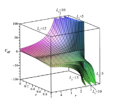
Figure 1: The plot of effective potential ($U_{\text{eff}}$) versus $r$ and $t$ for $\alpha=\epsilon=1$, $M=10^{-16}$.

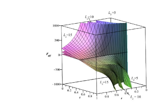
Figure 2: Plot of effective force versus $r$ and $t$ for $\alpha=\epsilon=1$, $M=10^{-16}$.

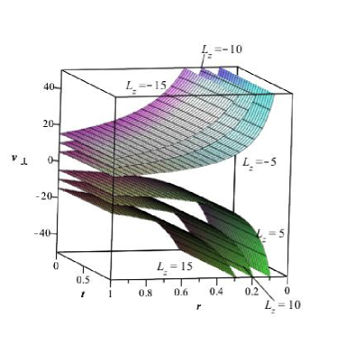
Figure 3: Plot of escape velocity versus $r$ and $t$ for $E=\alpha=\epsilon=1$, $M=10^{-16}$.

4.2 Behavior of Effective Force of Neutral Particle

The effective force is

$$F_{eff}=-\frac{1}{2}\frac{dU_{eff}}{dt}=-\frac{M}{r^{2}}\bigg{(}1-\frac{\epsilon t}{\alpha}+\frac{L_{z}^{2}\big{(}1-2\frac{\epsilon t}{\alpha}\big{)}}{r^{2}}\bigg{)}+\big{(}1-\frac{2M}{r}\big{)}\frac{L_{z}^{2}\big{(}1-2\frac{\epsilon t}{\alpha}\big{)}}{r^{3}}.$$ (42)

We are studying the motion of neutral particle in surrounding of Schwarzschild BH where attractive and repulsive gravitational forces produce by scalar vector tensor field which prevents a particle to fall into singularity [33]. The comparison of effective force on particle around Schwarzschild BH as function of radial coordinate for different values of angular momentum is shown in Figure 2. We can see from figure, at time interval $[0,0.5)$, the attraction of particle to reach singularity is more for $L_{z}=15$ as compared to $L_{z}=5,10$. Similarly, at time interval $(0.5,1]$, the repulsion of particle to reach the singularity is more for $L_{z}=15$ as compared to $L_{z}=5,10$. Also, at $t=0.5$ there is no effective force. Since $t=0.5$ acts as a shifting point, i.e., the effective force is shifting from attraction to repulsion at $t=0.5$. We can conclude that the attraction and repulsion of particle to reach and escape from singularity is more for large values of angular momentum but it mainly depend upon time.

4.3 Trajectories of Escape Velocity of Neutral Particle

Figure 3 represents the trajectories of escape velocity for different values of $L_{z}$ as a function of $r$. It is evident that if angular momentum is positive then escape velocity is repulsive while it is attractive for negative values of angular momentum. Also, the repulsion of escape velocity for large values of $L_{z}$ is strong as compared to small values of $L_{z}$. On the other hand, the attraction of escape velocity for $L_{z}=-15$ is strong as compared to $L_{z}=-5,-10$. We can conclude that escape velocity of particle increases as angular momentum increases but it becomes almost constant away from the BH. Also it is interesting that the trajectories of escape velocity do not vary with respect to time.

5 Dynamics of the Charge Particle

Now we consider the dynamics of charged particle around time conformal Schwarzschild BH defined by (1). We assume that a particle has electric charge and its motion is affected by magnetic field in BH exterior. Also, we assume that there exits magnetic field of strength $(\mathbb{B})$ in the neighborhood of BH which is homogenous, static and axisymmetric at spatial infinity. Next, we follow the procedure of [34] to construct magnetic field. Using metric (1), the general killing vector is [35]

$$\Box\xi^{\mu}=0,$$ (43)

where $\xi^{\mu}$ is killing vector. Using above equation in Maxwell equation for 4- potential $A^{\mu}$ in lorentz gauge $A^{\mu}_{;\mu}=0$, we have [36]

$$A^{\mu}=\frac{\mathbb{B}}{2}\xi^{\mu}_{(\phi)},$$ (44)

The killing vectors correspond to 4-potential which is invariant under symmetries as follows

$$L_{\xi}A_{\mu}=A_{\mu,\nu}\xi^{\nu}+A_{\nu}\xi^{\nu}_{,\mu}=0.$$ (45)

Using magnetic field vector [20]

$$\mathbb{B}^{\mu}=-\frac{1}{2}e^{\mu\nu\lambda\sigma}F_{\lambda\sigma}u_{\nu},$$ (46)

where $e^{\mu\nu\lambda\sigma}=\frac{\epsilon^{\mu\nu\lambda\sigma}}{\sqrt{-g}}$, $\epsilon_{0123}=1$, $g=det(g_{\mu\nu})$, $\epsilon^{\mu\nu\lambda\sigma}$ is Levi Civita symbol. The Maxwell tensor is

$$F_{\mu\nu}=A_{\nu,\mu}-A_{\mu,\nu}.$$ (47)

In metric (1), for local observer at rest, we have

$$u^{\mu}_{0}=\big{(}1-\frac{2M}{r}\big{)}^{-\frac{1}{2}}\xi^{\mu}_{(t)},u^{\mu}_{3}=(rsin\theta)^{-1}\xi^{\mu}_{(\phi)}.$$ (48)

The remaining two components are zero at $\dot{r}=0$ (turning point). From Eqs. (44) and (46), we get

$$\mathbb{B}^{\mu}=\mathbb{B}\big{(}1-\frac{2M}{r}\big{)}^{-\frac{1}{2}}\left(cos\theta\delta^{\mu}_{r}-\frac{sin\theta\delta^{\mu}_{\theta}}{r}\right),$$ (49)

here the magnetic field is directed along z-axis (vertical direction). Since the field is directed upward, so we have $\mathbb{B}>0$.

The Lagrangian of particle moving in curved space time is given by [37]

$$L=\frac{1}{2}g_{\mu\nu}u^{\mu}u^{\nu}+\frac{qA}{m}u^{\mu},$$ (50)

where $m$ and $q$ are the mass and electric charge of the particle respectively. The generalized 4-momentum of particle is

$$P_{\mu}=mu_{\mu}+qA_{\mu}.$$ (51)

The new constants of motion are defined as

$$\dot{t}=\frac{E(1-\frac{\epsilon t}{\alpha})}{\big{(}1-\frac{2M}{r}\big{)}},\quad\dot{\phi}=\frac{L_{z}(1-\frac{\epsilon t}{\alpha})}{r^{2}\sin^{2}\theta}-B,$$ (52)

where $B=\frac{q\mathbb{B}}{2m}$. Using the constraints in the Lagrangian (12) the dynamical equations for $\theta$ and $r$ become

$$\ddot{\theta}=\frac{\cos\theta(L_{z}(1-\frac{\epsilon t}{\alpha})-B)^{2}}{r^{4}\sin^{3}\theta}-2\frac{\epsilon\dot{\theta}Er}{\alpha(r-2M)}-4\frac{\dot{r}\dot{\theta}}{r},$$ (53)

$$\ddot{r}=\frac{3M\dot{r}^{2}}{r(r-2M)}-\frac{2\epsilon Er\dot{r}}{\alpha(r-2M)}-\frac{ME^{2}(1-\frac{2\epsilon t}{\alpha})}{r(r-2M)}+(r-2M)\bigg{(}\dot{\theta}^{2}+\sin^{2}\theta\big{(}\frac{L_{z}(1-\frac{\epsilon t}{\alpha})}{r^{2}\sin^{2}\theta}-B\big{)}^{2}\bigg{)}.$$ (54)

Using the normalization condition, we obtain

$$E^{2}=\dot{r}^{2}+r^{2}\big{(}1-\frac{2M}{r}\big{)}\dot{\theta}^{2}+\big{(}1-\frac{2M}{r}\big{)}\bigg{(}(1-\frac{\epsilon t}{\alpha})+r^{2}\sin^{2}\theta\big{(}\frac{L_{z}(1-\frac{\epsilon t}{\alpha})}{r^{2}\sin^{2}\theta}-B\big{)}^{2}\bigg{)}.$$ (55)

The effective potential takes the form

$$U_{eff}=\big{(}1-\frac{2M}{r}\big{)}\bigg{(}(1-\frac{\epsilon t}{\alpha})+r^{2}\sin^{2}\theta\big{(}\frac{L_{z}(1-\frac{\epsilon t}{\alpha})}{r^{2}\sin^{2}\theta}-B\big{)}^{2}\bigg{)}.$$ (56)

The energy of the particle moving around the BH in orbit $r$ at the equatorial plane is

$$U_{eff}=\big{(}1-\frac{2M}{r}\big{)}\bigg{(}(1-\frac{\epsilon t}{\alpha})+r^{2}\big{(}\frac{L_{z}(1-\frac{\epsilon t}{\alpha})}{r^{2}}-B\big{)}^{2}\bigg{)}.$$ (57)

This is a constraint equation i.e. it is always valid if it is satisfied at initial time. Let us discuss the symmetric properties of Eq.(54) which are invariant under the transformation as follows

$$\phi\rightarrow-\phi,L_{z}\rightarrow-L_{z},B\rightarrow-B.$$ (58)

Therefore, without the loss of generality, we consider $B>0$ and for $B<0$ we should apply transformation (58) because negative and positive both charges are inter related by the above transformation. However, if one choose positive electric charge $(B>0)$ then both cases of $L_{z}$ (positive and negative) must be studied. They are physically different: the change of sign of $L_{z}$ corresponds to the change in direction of Lorentz force acting on the particle [20].

The system (52) - (54) is also invariant with respect to reflection $\theta\rightarrow\pi-\theta.$ This transformation preserves the initial position of the particle and changes $v_{\bot}\rightarrow-v_{\bot}.$ Therefore it is sufficient to consider the positive value of escape velocity $(v_{\bot})$ [20]. By differentiating Eq.(57) with respect to $r$, we obtain

$$\frac{dU_{eff}}{dr}=\frac{2M}{r^{2}}\bigg{(}1-\frac{\epsilon t}{\alpha}+r^{2}\big{(}\frac{L_{z}(1-\frac{\epsilon t}{\alpha})}{r^{2}}-B\big{)}^{2}\bigg{)}-2rB\big{(}1-\frac{2M}{r}\big{)}\bigg{(}\frac{L_{z}(1-\frac{\epsilon t}{\alpha})}{r^{2}}-B\bigg{)}.$$ (59)

The effective potential after the collision when the body in the magnetic field ($\theta=\frac{\pi}{2}$ and $\dot{r}=0$) is

$$E^{2}=U_{eff}=f(r)\bigg{(}(1-\frac{\epsilon t}{\alpha})+r^{2}\big{(}\frac{(L_{z}+v_{\bot}r)(1-\frac{\epsilon t}{\alpha})}{r^{2}}-B\big{)}^{2}\bigg{)}.$$ (60)

The escape velocity of the particle takes the form

$$v_{\bot}=\bigg{[}\bigg{(}\frac{rE^{2}-(r-2M)(1-\frac{\epsilon t}{\alpha})}{r-2M}\bigg{)}^{\frac{1}{2}}+rB\bigg{]}(1+\frac{\epsilon t}{\alpha})-\frac{L_{z}}{r}.$$ (61)

Differentiating Eq.(59) again with respect to $r$ we have

$$\frac{d^{2}U_{eff}}{dr^{2}}=\frac{2M}{r^{2}}\big{(}1-\frac{\epsilon t}{\alpha}\big{)}+(4M-r)\bigg{(}\frac{L_{z}(1-\frac{\epsilon t}{\alpha})}{r^{2}}-B\bigg{)}^{2}.$$ (62)

5.1 Behavior of Effective Potential of Charged Particle

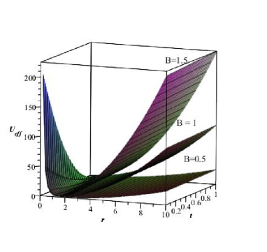
Figure 4: Graph of effective potential versus $r$ and $t$ given in Eq.(57) for $\alpha=\epsilon=1$, $M=10^{-16}$ and $L_{z}=3$.

Figure 4 represents the behavior of effective potential as a function of radial coordinate for different values of magnetic field B. The minima of effective potential at $B=0.5$ is approximately at $r=2$ initially but as time increase it shifting near the BH. Hence the presence of magnetic field increases the possibility of particle to move in stable orbit. Similarly, initially the minima of effective potential at $B=1,1.5$ is approximately at $r=1.5,1.25$ respectively, as time increases it approaches near BH. One can noticed that in the presence of low magnetic field, the minima of effective potential is shifted away from the horizon and width of ISCO is also decreased as compared to high magnetic field. These results is an agreement with [34, 38]. Therefore we can say that increase in magnetic field act as increase instable orbits of particle. Another aspect from figure is that at initial time, we have possibility of stable orbit but as time increases the possibility of ISCO getting low and at $t=1$, the stable orbit is lost. Hence it is possible that the particle is captured by the BH or it escape to infinity.

5.2 Behavior of Effective Force of Charged Particle

The effective force on the particle can be defined as as

$$F_{eff}=-\frac{1}{2}\frac{dU_{eff}}{dr}=-\frac{M}{r^{2}}\bigg{(}1-\frac{\epsilon t}{\alpha}+r^{2}\big{(}\frac{L_{z}(1-\frac{\epsilon t}{\alpha})}{r^{2}}-B\big{)}^{2}\bigg{)}+rB\big{(}1-\frac{2M}{r}\big{)}\bigg{(}\frac{L_{z}(1-\frac{\epsilon t}{\alpha})}{r^{2}}-B\bigg{)}.$$ (63)

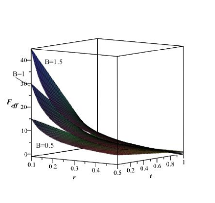
Figure 5: Graph of effective force versus $r$ and $t$ given in Eq. (63) for $\alpha=\epsilon=1$, $M=10^{-16}$ and $L_{z}=3$.

We have plotted the effective force for different values of B as function of $r$ . We see from Figure 5 that effective force is more attractive for large values of magnetic field as compared to small values. We can conclude that effective force of particle increases as strength of magnetic field increases near BH initially but with the passage of time, the particle moves away from BH it becomes almost constant.

5.3 Trajectories of Escape Velocity of Charged Particle

From Eq.(52), the angular variable we have

$$\dot{\phi}=\frac{L_{z}(1-\frac{\epsilon t}{\alpha})}{r^{2}\sin^{2}\theta}-B.$$ (64)

If the the Lorentz force on particle is attractive then left hand side of above equation is negative [39] and vice verse. The motion of charged particles is in clockwise direction. Our main focus on magnetic field acting on particle, the large value of magnetic field deforms the orbital motion of particle as compared to small values. Hence, we can conclude that the possibility to escape the particle from ISCO is greater for large values of magnetic field. We also explain the behavior of escape velocity for different values of magnetic field in Figure 6 graphically. The escape velocity of particle increases for large values of magnetic field as compared to small values. We can conclude that presence of magnetic field provide more energy to particle to escape from vicinity of BH. Figure 7 represents escape velocity against $r$ for different values of angular momentum. The possibility of particle to escape is low for large values of angular momentum. Also as time increases the possibility of particle to escape is decreasing drastically.

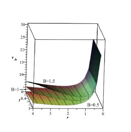
Figure 6: Plot of escape velocity versus $r$ and $t$ given in Eq.(61) for $E=\alpha=\epsilon=1$, $M=10^{-16}$ and $L_{z}=5$.

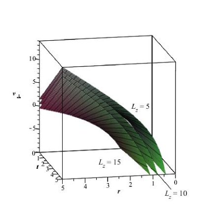
Figure 7: Plot of escape velocity versus $r$ and $t$ given in Eq.(61) for $E=\alpha=\epsilon=1$, $M=10^{-16}$ and $B=0.5$.

6 Stability Orbit

The Lyapunov function is defined as [40]

$$\lambda=\bigg{(}\frac{-U_{eff}^{{}^{\prime\prime}}(r_{0})}{2\dot{t}^{2}(r_{0})}\bigg{)}^{\frac{1}{2}}.$$ (65)

Using Eq.(62) we can get the Lyapunov function as

$$\lambda= \frac{\big{(}1+\frac{\epsilon t}{2\alpha}\big{)}(r-2M)}{r^{\frac{5}{2}}E}\bigg{[}2M\bigg{(}1+2L_{z}\big{(}\frac{(1-\frac{\epsilon t}{\alpha})L_{z}}{r^{2}}-B\big{)}\bigg{)}+B\bigg{(}rL_{z}-r^{3}B(1+\frac{\epsilon t}{\alpha})$$

$$- 2L_{z}(r-2M)\bigg{)}\bigg{]}^{\frac{1}{2}}.$$

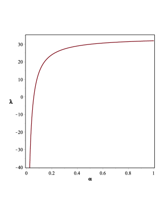
Figure 8: Lyapunov exponent as a function for $\alpha$ for $B=\epsilon=1$, $M=10^{-16}$, $L_{z}=??$, $r=1$and $t=1$.

Behavior of $\lambda$ as function of $\alpha$ is analyzed Figure 8. We can see from figure that instability of circular orbit increases as $\alpha$ increases but it becomes constant

7 Conclusion and Observations

In the present work, we found that one of the Noether symmetry admit approximated part. This symmetry is the translation in time which means that the energy of the spacetime is re-scaling. We also found the conservation laws corresponding to the exact Schwarzschild spacetime and the time conformal Schwarzschild spacetime and compare their numerical solutions. The geodesic deviation has also presented. The perturbation in the spacetime has perturbed the geodesic. The numerical solutions showed that how much they deviated from each other.

Using Noetherine symmetries, we have calculated the equation of motions. We have found three types of approximate Noether symmetries which correspond to energy, scaling and Lorentz transformation in the conformal plane symmetric spacetimes. These symmetries approximate the corresponding quantities in the respective spacetimes. We have not seen approximate Noether symmetries corresponding to linear momentum, angular momentum and galilean transformation in our calculations. This shows that these quantities conserved for plane symmetric spacetimes. The spacetime section of zero curvature does not admit approximate Noether symmetry [41] which shows that the approximate symmetries disappeared whenever we have the section of zero curvature in the spacetimes. However, the approximate Noether symmetry does not exist in flat spacetimes (Minkowski spacetime).

In addition, we have investigated the motion of neutral and charged particles in the absence and presence of magnetic field around the time conformal Schwarzschild BH. The behavior of effective potential, effective force and escape velocity of neutral and charged particles with respect to time are discussed. In case of neutral particle, for large values of angular momentum, we have found attraction and repulsion with respect to time as shown in Figures 1-3. This effect decreases far away from BH with respect to time. The more aggressive attraction and repulsion of particle to reach and escape from BH has been observed for large values of angular momentum due to time dependence. The escape velocity increases as angular momentum increasing but it does not vary with respect to time.

In case of charged particle, the presence of high magnetic field shifted the minima of effective potential towards the horizon and width of stable region is increased as compare to low magnetic field. Escape velocity for different values of angular momentum and magnetic field are shown in Figure 6-7. It is found that the presence of magnetic field provided more energy to particle to escape. The possibility of particle to escape is low for large angular momentum and as time increases it decreases continuously.

References

- [1] Frolov, V. P. and Novikov, I. D.: Black Hole Physics, Basic Concepts and New Developments, (Springer 1998).
- [2] Sharp, N. A.: Gen. Rel. Grav.10, 659 (1979).
- [3] Borm, C. V. and Spaans, M.: Astron. Astrophys. 553, L9 (2013).
- [4] Znajek, R.: Nature 262, 270 (1976).
- [5] Blandford, R. D. and Znajek, R. L.: Mon. Not. Roy. Astron. Soc. 179, 433 (1977).
- [6] Koide, S., Shibata, K., Kudoh, T., and Meier, D. l.: Science 295, 1688(2002).
- [7] Wachter S., et al.: Nature 453, 626 (2008).
- [8] Braithwaite, J. and Spruit, H. C.: Nature 431, 819 (2004).
- [9] Ferrario, L. and Wickramasinghe, D. T.: MNRAS 356, 615 (2005).
- [10] Lou, Y. Q. and Wang, W. G.: MNRAS 378, L54 (2007).
- [11] Lou, Y. Q.: MNRAS 275, L11 (1995).
- [12] Wang, W. G., Lou, Y.Q.: ApSS 315, 135 (2008).
- [13] Neronov, A. and Vovk, I.: Science 328, 73 (2010).
- [14] Vovk, I., Taylor, A. M., Semikoz, D. and Neronov, A.: Astrophys. J. 747, L14 (2012).
- [15] Mishra, K.N. and Chakraborty, D.K.: Astrophys. Spac. Sci. 260, 441 (1999).
- [16] Teo, E.: Gen. Relat. Grav. 35, 1909 (2003).
- [17] Hussain, S., Hussain, I. and Jamil, M.: Eur. Phys. J. C 74, 3210 (2014).
- [18] Babar. G. Z., Jamil, M. and Lim, Y.K.: Int. J. Mod. Phys. D 25, 1650024 (2016).
- [19] Pugliese, D., Quevedo, H. and Ruffni, R.: Phys. Rev. D 83, 104052 (2011).
- [20] Zahrani, A. M. A., Frolov, V. P. and Shoom, A. A.: Phys. Rev. D 87,084043 (2013).
- [21] Ali, F.: Applied Mathematical Sciences. 8, 4679 (2014).
- [22] Ali, F., Feroze, T. and Ali, S.: Theoretical and Mathematical Physics 184, 92 (2015).
- [23] Ali, F.: Mode. Phys. lett. A 30, 1550028 (2015).
- [24] Ali, F. and Feroze, T.: Int. J. Theor. Phys. 52(9), 3329 (2013).
- [25] Senovilla, J.M.M.: Gen. Relativ. Gravit. 29(1997)701.
- [26] Senovilla, J.M.M.: Inter. J. of Mod. Phys.: Conference Series 7(2012)1.
- [27] Bengtsson, I. and Senovilla, J.M.M.: Phys. Rev. D83(2011)044012.
- [28] Senovilla, J.M.M.: Class. Quantum Grav. 19(2002)L113.
- [29] D’Inverno, R.: Introducing Einstein s Relativity (Clarendon Press, Oxford, 1992)
- [30] Prestidge, T: Phys Rev D 61, 084002 (2000).
- [31] York, J.W.: Phys Rev D 33, 2092 (1986).
- [32] Chandrasekher, S.: The Mathematical Theory of Black Holes (Oxford University Press, 1983).
- [33] Moffat, J. W.: JCAP 0603, 3004 (2006).
- [34] Aliev, A. N. and Gal tsov, D. V.: Sov. Phys. Usp. 32(1), 75 (1989).
- [35] Wald, R.M.: Phys. Rev. D 10, 1680 (1974).
- [36] Aliev, A. N. and Ozdemir, N.: Mon. Not. Roy. Astron. Soc. 336, 241 (1978).
- [37] Landau, L. D. and Lifshitz, E. M.: The Classical Theory of Fields (Pergamon Press, Oxford, 1975).
- [38] Hussain, S., Hussain, I. and Jamil, M.: Eur. Phys. J. C 74, 3210 (2014).
- [39] Frolov, V. P. and Shoom, A. A.: Phys. Rev. D 82, 084034 (2010).
- [40] Cardoso, V., Miranda, A.S., Berti, E., Witech, H. and Zanchin, V.T: Phys. Rev. D 79, 064016 (2009).
- [41] Feroze, T. and Ali, F.: J. Jeom. Phys. 80, 88 (2014).