The Magnetic Field of L1544:
I. Near-Infrared Polarimetry and the Non-Uniform Envelope

Abstract

The magnetic field (B-field) of the starless dark cloud L1544 has been studied using near-infrared (NIR) background starlight polarimetry (BSP) and archival data in order to characterize the properties of the plane-of-sky B-field. NIR linear polarization measurements of over 1,700 stars were obtained in the $H$ band and 201 of these were also measured in the $K$ band. The NIR BSP properties are correlated with reddening, as traced using the RJCE ($H$ - $M$) method, and with thermal dust emission from the L1544 cloud and envelope seen in Herschel maps. The NIR polarization position angles change at the location of the cloud and exhibit their lowest dispersion of position angles there, offering strong evidence that NIR polarization traces the plane-of-sky B-field of L1544. In this paper, the uniformity of the plane-of-sky B-field in the envelope region of L1544 is quantitatively assessed. This allowed evaluating the approach of assuming uniform field geometry when measuring relative mass-to-flux ratios in the cloud envelope and core based on averaging of the envelope radio Zeeman observations, as in Crutcher et al. (2009). In L1544, the NIR BSP shows the envelope B-field to be significantly non-uniform and likely not suitable for averaging Zeeman properties without treating intrinsic variations. Deeper analyses of the NIR BSP and related data sets, including estimates of the B-field strength and testing how it varies with position and gas density, are the subjects of later papers in this series.

1 Introduction

Magnetic fields (B-fields) are present in the diffuse interstellar material from which dark, molecular clouds form. B-fields are also present in the cores of those clouds, some of which form new stars. Theoretical modeling of cloud and star formation in the presence of magnetic fields has a long, rich history Mestel & Spitzer (1956) which continues through recent work (e.g., Mouschovias, 1991; Galli & Shu, 1993; Basu & Mouschovias, 1994; Padoan & Nordlund, 1999; Mouschovias et al., 2006; Hennebelle & Fromang, 2008; Li et al., 2015) and comprehensive reviews (e.g., Mouschovias, 1996a, b). Observational tests of such theories have been rarer (e.g., Goodman et al., 1989, 1995; Crutcher, 1999; Crutcher et al., 2009; Zhang et al., 2014; Pillai et al., 2015), but are now advancing at an accelerated pace (see review by Li et al., 2014). A key quantity used to assess cloud stability and predict future outcomes is the ratio of mass, in the form of gas and dust, to the flux of the B-field threading that material. This ‘mass-to-flux’ ratio (e.g., Mestel & Spitzer, 1956; Mouschovias, 1976a, b; Fiedler & Mouschovias, 1992; Crutcher, 2012) is normally indexed by its critical ratio, the value at which the gravitational and magnetic energy densities are equal, yielding a $M/\Phi$ ratio of unity. If $M/\Phi$ is sub-unity, then B-fields dominate and the region is classified as sub-critical. If $M/\Phi$ exceeds unity, the region is super-critical, with B-fields overwhelmed by gravity, leading to contraction or collapse. The differential $M/\Phi$ of a cloud core relative to its envelope is a key indicator of the role of B-fields in star formation (Mouschovias, 1976a).

However, measuring $M/\Phi$ is challenging. Assessing the numerator involves sensing atomic or molecular gas densities, temperatures, and columns. This is made especially difficult when depletion onto dust grains robs the gas of the already rare species used as proxy tracers for the dominant H₂ gas. Tracing gas by using dust, as revealed through the reddening and extinction of starlight (or background diffuse emission) or via thermal emission from the dust grains, is less affected by depletion, though not fully immune. And, depending on the collision rate of gas and dust, the dust temperature may not closely reflect the gas temperature. Well-sampled, large-area gas spectral line maps, sensitive multi-wavelength dust maps, and multi-species, multi-line analyses over cloud envelope and core regions, where properties change rapidly with location, are necessary to address these difficulties.

Computing the denominator in $M/\Phi$ is even more difficult. The B-field is a three-dimensional vector field, yet current best methods can only probe either the line-of-sight component, $B_{LOS}$, employing the Zeeman effect for radio spectral line observations, or the plane-of-sky component, $B_{POS}$, using background starlight polarimetry (BSP) or linear polarization of the thermal dust emission. An alternate spectral line method, exploiting the Goldreich-Kylafis (1981) effect, may return more than single dimension information, but only in special anisotropic settings (e.g., Girart et al., 1999).

Radio Zeeman observations need significant gas column densities and relatively quiescent conditions to yield detectable signals within reasonable integration times. Hence, the number of targets observed using the Zeeman effect for the OH molecule, which is best for the typical conditions in molecular clouds (while CN is better for massive, star-forming cloud cores; Crutcher et al., 1996), is not large. The number of OH Zeeman effect detections is even smaller. Yet, the Zeeman effect directly returns the line of sight component of the B-field strength, making it a ‘gold standard’ tool for assessing cloud stability.

Polarized thermal dust emission in the mm, submm, and far-infrared (FIR) reveals the orientations of $B_{POS}$, but only where the emission (and the weaker polarization) can be detected. This favors the densest and warmest cloud core locations. Crutcher et al. (2004) compared the $B_{POS}$ amplitude, inferred from the Ward-Thompson et al. (2000) James Clerk Maxwell Telescope (JCMT) SCUBA (Holland et al., 1999) 850 $\mu$m polarization map, with the Crutcher & Troland (2000) OH Zeeman $B_{LOS}$ amplitude for L1544. That comparison indicated more than an order of magnitude discrepancy. Crutcher et al. (2004) attributed this to the different sizes of the structures traced by the two methods and to the dependence of field strength on density under flux-freezing conditions. A better approach, one that samples the same structures and densities as the Zeeman OH method, is needed.

Background starlight polarimetry, especially performed in the dust-penetrating near-infrared (NIR), reliably reveals B-field orientations in the plane-of-the-sky, and can do so with higher angular resolution and numbers of directions probed than available Zeeman observations. But, using BSP to develop B-field strengths, and so assess $M/\Phi$ ratios and cloud and core stability, depends on a longer and more complex chain of arguments. Nevertheless, the ease of obtaining BSP B-field maps offers the opportunity to gain insight into B-field properties over a remarkably wide range of diffuse and molecular cloud conditions.

1.1 The L1544 Laboratory

L1544 represents a nearly ideal laboratory for comparing the Zeeman and BSP methods. It is a molecular cloud with a starless dense cloud core (Snell, 1981; Myers et al., 1983; Heyer et al., 1987) in Taurus, at a distance of about 140 pc (Elias, 1978; Kenyon et al., 1994; Torres et al., 2012). Detection of ammonia by Myers & Benson (1983) and N₂H⁺, C₃H₂, and CCS by Benson et al. (1998) began a long history of interstellar chemistry and kinematic studies of L1544, as it supports an unusually chemical richness (e.g., Caselli et al., 2002a; Lee et al., 2003; van der Tak et al., 2005; Vastel et al., 2006; Bizzocchi et al., 2014), strong depletion of many species onto cold dust grains (Tafalla et al., 2002; Keto & Caselli, 2010), and rotation plus infall motions (Tafalla et al., 1998; Williams et al., 1999, 2006; Keto et al., 2015). L1544 was the first dark cloud core to be detected in the fundamental ortho-water transition using Herschel (Caselli et al., 2010) and continues to serve as a key laboratory for modeling water in dark clouds (Keto et al., 2014). Detailed modeling of the physical conditions, stability, ionization state, and magnetic properties of L1544 have been pursued in several studies (e.g., Ciolek & Basu, 2000; Tafalla et al., 2002; Li & Nakamura, 2002; Li et al., 2002; Crapsi et al., 2005; Keto & Caselli, 2008).

The strong depletion of CO isotopologues and the resultant uncertainty regarding the abundances of these species have favored observations of optically thin dust continuum emission for revealing the physical nature of the L1544 core and envelope regions. Studies include 1.3 mm mapping at IRAM by Ward-Thompson et al. (1999), 850 $\mu$m mapping by Shirley et al. (2000) and Ward-Thompson et al. (2000), and 450 $\mu$m mapping (Shirley et al., 2000; Doty et al., 2005). The Herschel satellite was used to map L1544 at 70, 100, 160, 250, 350, and 500 $\mu$m wavelengths in programs by O. Krause and P. André (obs IDs 1342193503/4 and 1342204841/2, respectively). These sensitive images reveal the L1544 cloud core and envelope with fine detail. Figure 1 shows the 250 $\mu$m Herschel/SPIRE map as the background image, with black contours stepped linearly with 250 $\mu$m intensity.

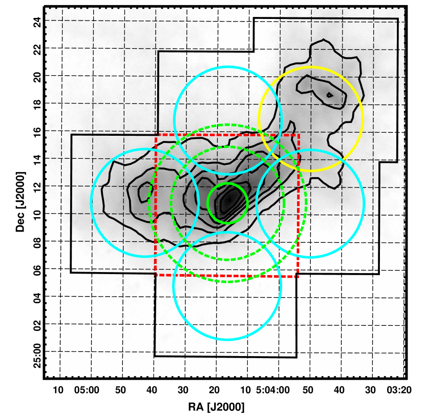
Figure 1: Gray-scale and contour map of Herschel/SPIRE 250 $\mu$m dust emission covering L1544. The dense cloud core is seen as the elongated, mostly gray to black structure in the figure center. Black contours start at 75 MJy sr^-1 and increase in steps of 25 MJy sr^-1. The solid green circle and dashed green circles identify the Arecibo main beam size (solid) and first sidelobe region (dashed) for the OH Zeeman observations of Crutcher et al. (2009). Four cyan circles identify the placements and beam size of their GBT OH Zeeman observations. The yellow circle identifies the placement and beam size of new Effelsberg OH Zeeman observations (K. Tassis 2016, private communication). The black polygon identifies the region surveyed for NIR $H$ band polarization while the red dashed box identifies the region surveyed for $K$ band polarization, both using Mimir in this current study.

The dust found in the dense cores of dark clouds like L1544 is optically thick at optical and near-infrared wavelengths and optically thin in the mid-infrared (Bacmann et al., 2000). The optically thin core of L1544 is easily seen as resolved, faint absorption in WISE (Wright et al., 2010) W3 (12 $\mu$m) and W4 (22 $\mu$m) maps of the region, which show the same orientation and structure exhibited by the bright FIR emission core of Figure 1.

The L1544 B-field strength was first measured via detection of the OH Zeeman effect by Crutcher & Troland (2000), who found $B_{LOS}=+11\pm 2$ $\mu$G using the Arecibo telescope along the direction to the cloud core in a nearly 16 hour integration. In the Arecibo OH Zeeman effect survey of 34 dark cloud cores (Troland & Crutcher, 2008), L1544 exhibits the second highest Zeeman signal-to-noise ratio (SNR), at 6.4. The fraction of survey targets with SNR $\geq$ 3 is only 21% and these used about 38% of the total integration time of the survey, underscoring the difficulty of determining B-field strengths from radio Zeeman observations.

To test predictions of ambipolar diffusion (AD) models (e.g., Ciolek & Mouschovias, 1994) for cloud core development leading to star formation, Crutcher et al. (2009) combined Arecibo OH Zeeman observations (beamsize $\sim 2.9$ arcmin) of four cloud cores with GBT OH Zeeman observations (beamsize $\sim 7.8$ arcmin) of their associated cloud core envelopes. The latter measurements were performed by sampling four positions located outside the Arecibo beam observation of each cloud core, with offsets along each equatorial cardinal direction of $\pm 6$ arcmin. The goal was to test whether the cloud cores and envelopes exhibited relative $M/\Phi$ ratios in excess of unity, as predicted by AD models. Of the four clouds observed, only a single envelope position toward L1544 exhibited a GBT Zeeman detection with SNR $\geq$ 3. Crutcher et al. (2009) averaged the four envelope GBT Zeeman values for each cloud to increase the SNR and thereby permit estimating or limiting envelope $M/\Phi$ values. However, this approach was criticized by Mouschovias & Tassis (2010) on the basis of likely non-uniformity of the envelope B-fields over the angular extent of the regions sampled by the GBT beams, based on the appearance of the Herschel and Spitzer dust thermal emission distributions on the sky for L1544 and the other three dark clouds.

Submm dust emission polarization at 850 $\mu$m was sought in the L1544 core by Ward-Thompson et al. (2000), who used JCMT with SCUBA and its polarimetry module (Greaves et al., 2003, hereafter ‘SCUPOL’). They obtained detections toward eight Nyquist-sampled directions, all within the Crutcher et al. (2009) Arecibo core OH Zeeman beam. One star (identified as 2MASS PSC J05041591+251157) just outside the core OH Zeeman beam was measured for $K$-band polarization by Jones et al. (2015).

Based on the condensed, quiescent, starless nature of its dense core, the presence of a resolved envelope, and the two, independent OH Zeeman detections of B-fields (toward the core and toward one envelope position), L1544 appears to be an ideal laboratory for conducting deep, NIR BSP observations and for the analyses of the resulting B-field orientations. Heretofore, no independent probe of the envelope B-fields has been reported for any of the four dark clouds studied using the OH Zeeman effect by Crutcher et al. (2009). The NIR BSP project described here was performed to directly addresses the nature of the envelope B-field in L1544.

1.2 Goals and Methodology

The first project goal was to obtain NIR BSP detections in regions that fully covered the portions of L1544 observed by the Arecibo and GBT OH Zeeman observations, to enable the desired polarization and B-field comparisons. NIR wavelengths (Section 2) offer good sensitivity for polarization detections toward regions of moderate dust extinction (A${}_{V}\sim 1-2$ mag) up to the much higher values (20 – 30 mag) characterizing the outer parts of dense cloud cores, through which optical starlight cannot penetrate. This observational goal was met through use of the Mimir NIR imaging polarimeter (Clemens et al., 2007) to deeply probe the L1544 core and to less deeply probe five fields offset from the core, four along the same cardinal directions as those of the GBT OH observations (Crutcher et al., 2009), and one to cover the region examined in recent radio Zeeman OH observations conducted at Effelsberg (K. Tassis 2016, private communication). BSP was performed over all these fields in the NIR $H$-band (1.6 $\mu$m) and also toward the center field in the NIR $K$-band (2.2 $\mu$m). These observations and the data reduction details are described in Section 2, below.

The second project goal was to demonstrate that the NIR polarizations returned by the Mimir observations revealed the B-field associated with L1544 and its core. Such association of BSP and molecular cloud B-fields has been challenged by Arce et al. (1998) as being due only to a ‘skin depth’ effect, though Whittet et al. (2008) found little evidence of such an effect. In Section 3, descriptions are presented of two tests that were performed to confirm the association of BSP and the B-field of L1544. The first test showed that NIR BSP is correlated with stellar reddening for the same stars and that this reddening is correlated with the dust thermal emission from L1544. The second test showed that the BSP-traced B-field properties of polarization position angle, PA, and dispersion of polarization position angle, $\Delta_{PA}$, exhibit strong spatial correspondences with the L1544 dust maps.

Section 4 presents an assessment of the mean BSP-traced $B_{POS}$ properties measured in synthetic beam averages representing the Zeeman radio beams (the same angular sizes and directions) used by Crutcher et al. (2009). This included analyzing possible non-uniformity of the envelope $B_{POS}$. This has impact on a key assumption underlying the Crutcher et al. (2009) envelope-averaging of Zeeman data, on their resulting conclusions regarding $M/\Phi$, and thus on their test of ambipolar diffusion.

In later papers in this series, the NIR BSP data are used to develop a map of BSP-traced B-field strength. This map is compared to the Arecibo and GBT OH Zeeman-traced B-field strengths of Crutcher et al. (2009), as well as new OH Zeeman observations conducted at the 100 m Effelsberg telescope to assess the degree of correspondence between the two techniques. A map of $M/\Phi$ across L1544 is also used to reassess the Crutcher et al. (2009) conclusions regarding AD in L1544.

2 Observations and Data Processing

Near-infrared imaging polarimetric observations of L1544 were conducted on the UT nights of 2013 January 20, 2015 October 27 and 31, 2015 November 1 and 2, and 2016 January 27 and 31 using the Mimir instrument (Clemens et al., 2007) on the 1.83 m Perkins Telescope, located outside Flagstaff, AZ. Mimir polarimetry used cold, rotated, compound half-wave plates (HWP) for modulating the polarization signal for each of the $H$ and $K$ wavebands and a fixed wire-grid analyzer preceding the $1024\times 1024$ pixel InSb ALADDIN III detector array. All polarization and reimaging optics in Mimir operated at 60-70 K and the detector array was at 33.5 K. The plate scale was 0.58 arcsec per pixel, resulting in a $10\times 10$ arcmin field of view (FOV). All observations were conducted through fewer than 1.4 airmasses and the seeing was better than 2 arcsec for all observations.

The observations, in each of the two bands, were performed by obtaining an image through a fixed angular orientation of the HWP then rotating the HWP to other angles and obtaining additional images. A total of 16 HWP angle-images, chosen to permit forming four independent sets of Stokes $U$ and $Q$ parameters for each star, were observed at each telescope pointing. The telescope performed a set of six sky pointings (as a rotated hex pattern), with 16 HWP angle-images obtained at each pointing, resulting in 96 images per observation.

Six pointing centers (‘fields’) were selected toward a Center direction ($\alpha=05^{h}$04^m16^s.6, $\delta=+$25$\arcdeg$10^′48^′′ [J2000]), the four equatorial NSEW directions offset by 6 arcmin from the Center, and one field to the NW offset mostly diagonally by about 10.9 arcmin. In the $H$ band, the observation sets included one dithered observation, at 2.5 s per exposure, toward each of the five fields. The four NSEW fields were also observed with four longer (15 s per exposure) polarimetric observations in the $H$ band. The NW field had eight 15 s per exposure $H$ band polarimetric observations. The Center field had one 2.5 s per exposure $K$ band observation, two 15 s per exposure $K$ band observations, an additional 2.5 s $H$, plus four 10 s and eight 15 s per exposure $H$ band observations. The total integration times were thus about 1.7 hours in $H$ band for each NSEW field, 3.6 hours in the NW field in $H$, 0.9 hours in $K$ toward the Center field, and 4.5 hours in $H$ toward the Center field. The shorter exposures served the purpose of extending the observational dynamic range to stars whose brightness would saturate in the longer exposures. The longer Center and NW integration times partially offset the higher extinctions present in these fields.

Calibration consisted of application of detector linearity and dark current corrections, in-dome polarization flat-fields in each band, as well as super-sky flat-fielding using the observed images, correction for secondary instrumental polarization across the FOV (determined from observations of mostly unpolarized globular cluster stars located off the Galactic plane), and HWP offset angle correction (determined from observations of polarization standard stars). Details of the observation methodology, data correction steps, and calibration are described in Clemens et al. (2012a, b).

The long (10s or 15s) observations for each band were combined to yield deep photometric images and polarimetric point source catalogs. The short (2.5s) observations were also processed to polarimetric point source catalogs. The short and long polarimetric catalogs were combined by matching star positions and computing variance-weighted mean $U$ and $Q$ values and deriving from them polarization percentages, $P$, and PA values and uncertainties. (All $P$ values and PA uncertainties, $\sigma_{PA}$, were corrected for the effects of positive bias in $P$, following Wardle & Kronberg (1974).)

The combined $H$ band polarimetric point source catalog had 1,712 entries, while the $K$ band catalog had 201 entries. The latter is smaller because of the smaller solid angle observed in $K$ band (29% of the $H$ band solid angle), the much shorter net integration time in $K$ band (20% of the $H$ band integration time), the lower mean polarizations in $K$ compared to $H$ ($\sim$ 60%, see below) for normal ISM dust (Serkowski et al., 1975), and the higher net extinction in the Center field compared to the NSEW fields (see Figure 1). The positions of all of the $K$ band stars matched to $H$ band stars.

In addition, the AllWISE (Cutri et al., 2013) catalog entries for the field shown in Figure 1 were fetched using DS9 (Joye & Mandel, 2003) to query the Centre de Données astronomiques de Strasbourg (CDS), resulting in 3,616 stars with at least a WISE W1 (3.6 $\mu$m) band or W2 (4.5 $\mu$m) band detection. These were positionally matched to the $H$ band catalog, yielding 1,262 matches. The properties of the 450 $H$ band stars without WISE star matches and the WISE stars without $H$ band star matches were similar in being fainter than the subset of stars with $H$-to-WISE matches. As the fainter stars in the $H$ band polarimetric catalog were not expected to yield polarization detections providing significant B-field information (Clemens et al., 2012a, c), this 26% non-match rate among the faint stars should not bias any findings based on the brighter stars.

Table 1: Stellar Polarimetry and Photometry in the L1544 Field

		Mimir Values / Uncertainties										2MASS Values / Unc.			WISE Values / Unc.
No.	RA/decl	$H$	$P^{\prime}_{H}$	PAH	$Q_{H}$	$U_{H}$	$K$	$P^{\prime}_{K}$	PAK	$Q_{K}$	$U_{K}$	$J$	$H$	$K$	W1	W2	Notes
	[$\arcdeg$]	[mag]	[%]	[$\arcdeg$]	[%]	[%]	[mag]	[%]	[$\arcdeg$]	[%]	[%]	[mag]	[mag]	[mag]	[mag]	[mag]
0001	75.84865	15.615	8.053	42.6	0.797	9.684	20.000		0.0	0.000	0.000	16.232	15.511	15.193	15.363	15.692
	25.26836	0.037	5.437	19.3	5.504	5.437	99.999		180.0	100.000	100.000	0.099	0.109	0.134	0.047	0.146
0002	75.84951	16.313	8.781	8.2	11.058	3.262	20.000		0.0	0.000	0.000	20.000	20.000	20.000	15.796	15.857
	25.36376	0.058	7.471	24.4	7.468	7.496	99.999		180.0	100.000	100.000	99.999	99.999	99.999	0.060	0.162
$\sim$
0455	75.98059	12.889	1.447	62.4	-0.840	1.205	12.640		27.0	1.718	2.365	13.683	13.000	12.716	12.554	12.480
	25.18452	0.010	0.249	4.9	0.250	0.248	0.017		21.0	2.055	1.527	0.034	0.032	0.025	0.024	0.026
$\sim$
0605	76.00536	11.766	0.000	0.0	-0.155	-0.057	20.000		0.0	0.000	0.000	12.444	11.815	11.658	11.448	11.388
	25.03555	0.001	0.462	180.0	0.460	0.479	99.999		180.0	100.000	100.000	0.045	0.037	0.027	0.053	0.055
0606	76.00553	10.350	0.142	47.3	-0.015	0.188	20.000		0.0	0.000	0.000	10.893	10.422	10.243	10.158	10.136	a
	25.03394	0.001	0.124	25.1	0.123	0.124	99.999		180.0	100.000	100.000	0.031	0.036	0.025	0.028	0.028

Note. — This is a shortened version of the full table that is available in electronic form, with the rows shown here containing entries with, and without, $K$-band polarimetry and $WISE$ photometry.

The combined data set of 1,712 stars is listed in Table 1. In the Table, the first column lists the star number and the second column presents the RA and decl on successive lines. Columns 3 – 7 list the Mimir-based $H$ band photometric magnitude, (debiased) linear polarization percentage, $P^{\prime}_{H}$, (equatorial) polarization PA_H (in deg E from N), and Stokes $Q_{H}$ and $U_{H}$ percentages. Columns 8 – 12 list the Mimir $K$ band values of magnitude, $P^{\prime}_{K}$, PA_K, $Q_{K}$, and $U_{K}$ for the 201 matching stars. Values of 20.000 in the $K$ band mag column signify the absence of a matching star. For those stars, the corresponding $P^{\prime}$ entry was set to zero, $\sigma_{P}$ was set to 99.99%, and PA was set to zero, with $\sigma_{PA}$ set to 180.00°. Uncertainties are found in the line immediately following a line of values.

For stars matched to 2MASS (Skrutskie et al., 2006; Cutri et al., 2003) point sources, columns 13 – 15 provide the $J$, $H$, and $K$ band magnitudes, with their uncertainties in the same columns on the following line. Where no magnitude is available, a value of 20.000 and uncertainty of 9.999 are inserted. The 1,262 WISE W1 and W2 band magnitudes are provided in columns 16 and 17, also following the convention that a missing magnitude is replaced with a value of 20.000 and uncertainty 9.999. The final column lists letters linked to notes following the Table.

Stellar polarizations obtained using imaging surveys, as performed here, result in wide ranges of polarimetric uncertainties, due to stellar faintness and sky brightness, as described in Clemens et al. (2012c). Users of Table 1 are cautioned to consider the biases in such data.

3 Analysis

3.1 Do NIR Polarizations Reveal the L1544 B-field?

Establishing the nature of the B-field in L1544 from NIR BSP rests on showing that the lines of sight to the background stars sample dust in the L1544 cloud and core and that the polarizations originate in that dust. In the past, BSP for other Taurus clouds has been argued to be incapable of revealing B-fields within the clouds, but instead reveals only those B-fields residing on the surfaces of the clouds (Arce et al., 1998). In the following, the Table 1 data set is shown to probe the L1544 envelope and core dust and the B-fields there. This begins by developing a map of stellar reddening and comparing to the Herschel thermal dust emission of the cloud (Figure 1). In the second phase, unique cloud physical characteristics are shown to correlate with unique polarization properties changes - conditions unlikely to obtain unless the B-field of the cloud also participates in those changes and is traced by the BSP up through extinctions as high as A${}_{V}\sim 40$ mag.

3.1.1 Stellar Reddening Map

The Rayleigh-Jeans Color Excess (RJCE) method of Majewski et al. (2011) reveals the stellar reddening caused by interstellar dust from $H$ and $M$ (4.5 $\mu$m) band magnitude differences, as compared to intrinsic $(H-M)$ stellar colors. RJCE is superior to similar techniques that do not use the $M$ band, because of the narrower range of intrinsic stellar colors and because $M$ band easily penetrates most dark clouds. The data set in Table 1 were used to develop $(H-M)$ colors from the Mimir, 2MASS, and WISE magnitudes. These colors were interpolated to create a map of reddening, as described in what follows.

There are 772 stars in Table 1 simultaneously having 2MASS $H$ and WISE W2 magnitude uncertainties smaller than 0.5 mag, resulting in that many $(H-M)$ colors with uncertainties below 0.7 mag. There are another 386 stars in the Table without such 2MASS $H$ band data, but which have good W2 band data. Their Mimir $H$ band magnitudes, which are normally not color-corrected but are matched to 2MASS $H$ zero points in each field (Clemens et al., 2012a), can be used if color-corrected. This was implemented by finding the zero-point $(H_{Mimir}-H_{2MASS})$ and the color term $(H_{2MASS}-W2)$ dependences on $(H_{Mimir}-W2)$. The final combined set of $(H-M)$ colors contained 1,158 stars, distributed mostly uniformly across the region.

This Mimir survey region area of about 420 sq arcmin, sampled by 1,158 stars, results in just under three measured stellar reddenings per sq arcmin. Interpolation onto a $10\times 10$ arcsec grid included weighting each star’s color by its inverse color variance and gaussian-tapered offset from each grid center. The effective angular resolution of the resulting $(H-M)$ color map was set by the stellar search radius from each grid center, the gaussian offset taper, and a final gaussian smoothing of the gridded interpolation. The effective number of stars used in the calculation of the interpolated reddening at each grid center was also found. At a resolution of 120 arcsec FWHM, no fewer than two stars were used to estimate color at each grid point (this was in the most opaque part of the cloud core) and a mean of 10 to 11 stars characterized the grid center color estimates across the map.

Figure 2 shows the resulting $(H-M)$ map. The gray-scale image fills the Mimir survey region (outlined in black). White contours run from 0.6 through 3.3 mag of $(H-M)$ color. The blue, filled, circles show the locations of the 1,158 stars. The reddening structure revealed in this map closely follows the location and structure of the Herschel  250 $\mu$m dust emission shown in Figure 1, including the general location of the dense core, the lower density extension running from the core to the west-northwest (i.e., L1544-W; Tafalla et al., 1998), and the partially detached lower density feature located east of the core (i.e., L1544-E; Tafalla et al., 1998). Thus, the BSP stellar polarization sample of Table 1 is well-suited to probing the dust and gas structure of the L1544 dark cloud.

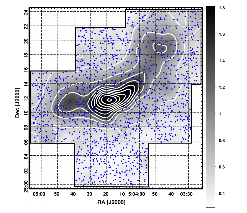
Figure 2: Gray-scale NIR stellar reddening map, computed from $(H-M)$ colors across the Mimir survey region. Grayscale wedge at right indicates mapping of darkness to $(H-M)$ color, in magnitudes. White contours begin at 0.6 mag and are stepped by 0.3 mag to a maximum of 3.3 mag (A${}_{V}>25$ mag). Blue filled circles identify the locations of the stars used to form the interpolated map. The highest reddening is offset from the FIR dust emission center (see Figure 1) because of the dearth of background stars visible through that center. The outer three contours closely follow the Herschel 250 $\mu$m dust emission structure, confirming that the emitting dust is also extincting and (as will be shown below) polarizing.

Interestingly, the region of Figure 2 showing $(H-M)$ colors bluer than 0.6 mag (i.e., outside the outermost contour) still shows significant color of about 0.4 mag. For an average intrinsic $(H-M)$ color of 0.08 mag (Majewski et al., 2011), the color excess is 0.32 mag, equivalent to A${}_{K}=0.29$ mag or A${}_{V}=2.2$ to $2.6$ mag (depending on the extinction curve chosen, as embodied in different $R_{V}$ values), distributed throughout the region surrounding L1544. The greatest reddening contour in Figure 2 is offset from the peak emission in Figure 1 for two reasons. First, the blue dot pattern shows that there are no Table 1 stars with $(H-M)$ colors located within 120 arcsec of the direction of the strongest FIR thermal dust emission, leaving the interpolated reddenings there based on the surrounding stars. Second, the star closest to the central contour has the greatest $(H-M)$ color of the sample, at 5.5 mag (A${}_{V}\geq 40$ mag), affecting or biasing the contour locations to some degree. Nevertheless, outside the very core, the stellar reddenings closely follow the dust thermal emission structure, giving high confidence that these stars can probe the B-field in their directions.

3.1.2 Foreground Star Census

One potential concern involves the possible biasing effects of including polarization values for stars located in the foreground with those for stars behind the cloud. Foreground stars in this field were sought using proper motion screening and color plus polarization screening. Thirteen stars exhibit proper motions in UCAC3 (The Third U.S. Naval Observatory CCD Astrograph Catalog; Zacharias et al., 2010) with SNRs in either RA or decl exceeding 2.5. Of these, all but two have $(H-M)$ colors that are redder than the extended region value of 0.4 mag, and were thereby judged to be background to the cloud. One of the survivors has $H=16.2$ mag (i.e., is quite faint) and $\sigma_{PA}$ of 60$\arcdeg$  (i.e., has a poorly constrained polarization PA) and so is unlikely to affect polarization findings no matter its location classification. The lone remaining star (number 606 in Table 1) with detectable proper motion ($0.42\pm 0.04$ arcsec per year) has $m_{H}=10.4$ mag, $(H-M)=0.22$ mag, and $P=0.14\pm 0.12$ %. Such low reddening and low polarization from a relatively bright star with measurable proper motion make it almost certainly a foreground star.

Other similar stars were sought in the $(H-M)$ subsample of Table 1, through color and polarization selections (stars bluer than some color limit and less polarized than some polarization limit). However, all such cuts returned samples of potential foreground stars that failed to be uniformly distributed across the Mimir survey region. In particular, all selections resulted in trial samples that avoided the high extinction zone of L1544. If there were significant numbers of foreground stars, some fraction of them should be projected against the mostly opaque core. Instead, no stars bluer than $(H-M)$ of 0.6 mag appear within any 0.8 mag contour in the $(H-M)$ image.

Hence, only one foreground star was detected with certainty, no significant population of foreground stars brighter than $H\sim 14$ can be present, and foreground stars fainter than 14th mag are likely to be only a few and will offer nearly zero contribution to the polarization maps and interpretations thereof. As a result, corrections for foreground extinction and polarization were deemed unnecessary.

3.1.3 $K$-Band Polarizations

The restricted solid angle observed for $K$-band polarization and the shorter integration times yielded only 201 stars with Mimir-measured polarizations in this band. Yet they provide important checks of the nature of the B-field and dust grains along these lines of sight. If polarization properties changed significantly as a function of wavelength or dust column density, reflected here in $(H-M)$ reddening, then disentangling changes in dust properties from changes in B-field properties would be more complex. The $K$ band polarization values were therefore compared to the $H$ band polarizations values to assess their correlation.

A subsample of the 201 $K$-band stars was selected based on requiring that $\sigma_{PA}$ in both $H$ and $K$ be below 30$\arcdeg$, to select good, or better quality data. This yielded 39 stars. For these, the variance-weighted (from propagated uncertainties) mean band ratio of polarization percentage and the mean band difference in position angles were found to be $P_{K}/P_{H}=0.62\pm 0.04$ and $\mathrm{PA}_{H}-\mathrm{PA}_{K}=8.9\pm 1.7\arcdeg$, respectively. The polarization ratio is higher than values expected for dust grains obeying the Serkowski Law of polarization versus wavelength (Serkowski et al., 1975; Wilking et al., 1980) and having $\lambda_{MAX}$ (the wavelength of maximum polarization) in the range 0.3 – 0.8 $\mu$m that is typically found (Wilking et al., 1980). Instead, values of $\lambda_{MAX}$ in the 1.0 – 1.2 $\mu$m range would be needed. Hence, the elevated $P_{K}/P_{H}$ ratio signifies that grain growth has taken place. This agrees with the strong depletion of gas phase molecules known to occur in L1544 (Caselli et al., 2002b).

The position angle offset is rather less revealing. The small offset from zero could be reflective of remnant $K$ band HWP zero angle calibration, which was based on far fewer observations of many fewer standard stars than for the extensive $H$ band calibration performed to support the GPIPS project (Clemens et al., 2012b). Alternatively, it could signify small changes in B-field and dust properties along the line-of-sight (Messinger et al., 1997).

Dependence on reddening, a proxy for dust column density, was examined via polynomial trial fits of $P_{K}/P_{H}$ versus $(H-M)$ color, and the same polynomial trial fits for $\mathrm{PA}_{H}-\mathrm{PA}_{K}$ versus that color. F-tests showed that no significant linear or higher terms were detectable in the 39 member stellar subsample, and thereby likely in the remainder of the sample. Interestingly, there is no difference in the $P_{K}/P_{H}$ ratio when the stars are split into a high reddening ($(H-M)>0.9$ mag) and a low reddening sample. This implies that grain growth must have also occurred in the cloud envelope or periphery, as well as in the dense core.

The overall conclusion is that dust properties along the lines of sight probed by both $H$ band polarization and $K$ band polarization are similar. There is no evidence of major dust property changes that would prevent B-field interpretations of the measured polarization position angle values, this despite the evidence for larger than normal grains. The uncertainties in the $K$ band polarization data are significantly larger than the $H$ band polarization data for the same stars, so much so that combining the PAs measured in the two bands, when weighted by their inverse variances, are indistinguishable from the $H$ band values alone. Hence, for most of the remainder of the analyses, only the $H$ band polarization properties are analyzed and reported (though the $K$ band values remain in Table 1 to support other studies). The $K$ band data are included in the final test of $B_{POS}$ properties across the GBT Zeeman beams, in Section 4.2.

3.1.4 Stellar PA Map

Figure 3 displays the $H$ band polarization position angles for the 396 stars in Table 1 having $\sigma_{PA}\leq 20\arcdeg$. These are grouped by $\sigma_{PA}$ value and coded into line segment (‘vector’) color, thickness, and length groups to better identify the highest quality values. The 123 stars with $\sigma_{PA}\leq 10\arcdeg$ have longer, thicker, red colored vectors. The middle 122 stars, with $\sigma_{PA}$ between 10 and 15$\arcdeg$ have average length, average thickness, magenta colored vectors. The 151 stars with $\sigma_{PA}$ between 15 and 20$\arcdeg$ have shorter, thinner, blue colored vectors. Together, these 396 stars represent the 23% of the full sample having the lowest $\sigma_{PA}$ values. In addition to the colored vectors, the Herschel 250 $\mu$m dust emission contours from Figure 1 are reproduced here to begin the association of NIR polarization vector properties with dust emission properties in L1544.

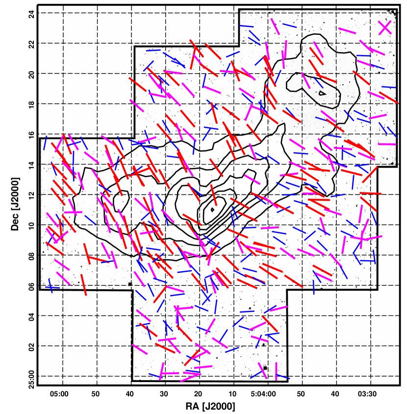
Figure 3: Gray-scale $H$ band image mosaic of Mimir surveyed region. Black contours indicate the Herschel  250 $\mu$m dust emission of Figure 1. Colored line segments (‘vectors’) display the $H$ band PAs and $\sigma_{PA}$, for subsets drawn from Table 1. Thicker, longer, red vectors display PA orientations for the 123 stars having $\sigma_{PA}\leq 10\arcdeg$. Medium thick, medium length, magenta vectors are for the 122 stars with $\sigma_{PA}$ between $10-15\arcdeg$. Thinner, shorter, blue vectors are for the 151 stars with $\sigma_{PA}$ between $15-20\arcdeg$. The PAs show significant star-to-star correlation while also revealing large-scale variation in overall PA orientations across the survey region.

The large number of vectors reveals several clear trends in the polarization properties. First, there is a high degree of correlation of PA orientations among neighboring stars. This basic uniformity is one of the best indicators that a large-scale B-field is being revealed across many pc of cloud extent. Second, there is an apparent change in mean PA across the surveyed region. In the western zone, the PAs are more nearly horizontal ($\sim$65$\arcdeg$ PA) while in the eastern zone, they are more nearly vertical ($\sim$25$\arcdeg$ PA). Hence, the mean field direction, as projected onto the plane of the sky, is seen to change in the region of the L1544 cloud and core. Third, the PAs seen for stars projected behind the strongest dust emission zones are not greatly different in orientation than those seen just outside those zones. Fourth, the dispersion in PA values among local vectors varies with position across the map. The eastern zone shows a high degree of star-to-star PA agreement, and thus a small PA dispersion, while the southern and northern zones show stronger local variations of PAs.

3.1.5 NIR BSP $P$, PA, and $\Delta_{PA}$ Smoothed Images

Spatial means of the NIR BSP values were developed to allow detailed comparison of the L1544 B-field properties with the gas and dust distribution. As was done for the $(H-M)$ map, weighted mean properties were computed on 10 arcsec spaced grid centers, including all stars out to 2.3 arcmin away from each center, and using inverse variance weighting and gaussian tapering by each star’s offset from the grid centers. This gaussian taper width ($\sigma$) was set to 1 arcmin, to favor values for stars located closest to the grid centers. The values computed at each grid center were created from as few as 7 stars (at the opaque cloud core) to as many as 34 stars. The mean number of stars per grid center was 16.6. The grid was smoothed with a second gaussian ($\sigma=50$ arcsec), yielding images with 3 arcmin FWHM resolution, comparable to the Arecibo Zeeman beamsize used by Crutcher et al. (2009), and much smaller than the GBT Zeeman beamsize.

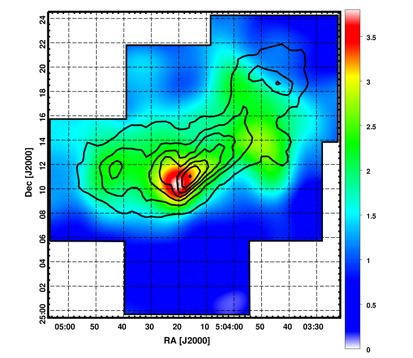
Figure 4: False-color map of mean $H$ band polarization percentage, $P^{\prime}_{H}$, across L1544, smoothed to 3 arcmin FWHM angular resolution. Color look-up wedge at right indicates the mapping of $P^{\prime}_{H}$ (in percent) to displayed colors. Black contours show the Herschel  250 $\mu$m emission displayed in Figures 1 and 3.

Figure 4 displays an image of the mean NIR $H$ band polarization percentage ($P^{\prime}_{H}$) distribution, and includes contours of the 250 $\mu$m dust emission traced by Herschel. Though there are some small differences (the NIR BSP is too extincted to probe the brightest 250 $\mu$m core emission), overall the NIR BSP polarization percentage is significantly enhanced where L1544 dust emission is strongest. Thus the NIR polarizations are tracing the B-field embedded in the same dust that is emitting at submm wavelengths. There appear to be three spatial peaks in the $P^{\prime}_{H}$ map: a strong peak at the dust emission center; a weaker peak offset by 8 arcmin to the NW (South of L1544-W); and another weaker peak offset by 5.5 arcmin to the ENE (L1544-E).

The dispersion in polarization position angle, $\Delta_{PA}$, is a measure of the degree to which background starlight reveals variations in the plane-of-sky B-field PAs. Figure 5 displays the spatial distribution of $\Delta_{PA}$, compared to the Herschel  250 $\mu$m dust emission. The map was computed similarly to the $P^{\prime}_{H}$ map, measuring PA dispersions with the same 3 arcmin FWHM resolution. This effectively removes the effects of any PA orientation changes on angular scales larger than this, but includes in the computed dispersions any changes on scales smaller than 3 arcmin. Also, the biasing effects of the individual stellar angular uncertainties in the overall PA dispersions were removed in quadrature, using a procedure similar to that used for SCUPOL data by Crutcher et al. (2004). In the Figure, note that the false-color scale is inverted to highlight where $\Delta_{PA}$ values are small, as might indicate higher B-field strengths according to the Chandrasekhar-Fermi (1953; hereafter ‘C-F’) method.

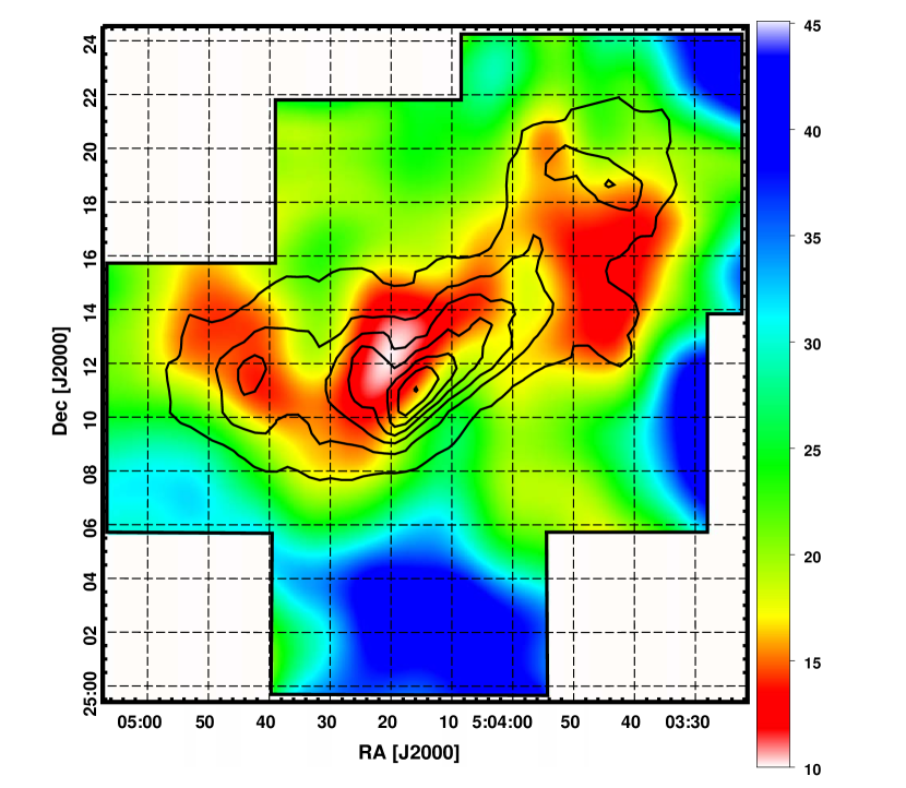
Figure 5: False-color map of $H$ band polarization position angle dispersion, $\Delta_{PA}$ (in degrees), across L1544, at 3 arcmin FWHM effective angular resolution. Color look-up wedge at right indicates mapping of $\Delta_{PA}$ to displayed colors. Black contours show the Herschel  250 $\mu$m emission.

The minimum $\Delta_{PA}$ value is just under 10$\arcdeg$ in the cloud core, and minima of 13$\arcdeg$  are seen very near the $P^{\prime}_{H}$ maxima locations to the ENE and NW. Thus, $P^{\prime}_{H}$ maxima and $\Delta_{PA}$ minima arise in the same material, likely signifying where conditions are quiescent and the B-field is more uniform and perhaps stronger. The NIR BSP $\Delta_{PA}$ features are correlated with the Herschel  250 $\mu$m emission, though there does appear to be somewhat of an offset along the ‘spine’ of the cloud. The sense of the displacement is that the minimum in $\Delta_{PA}$ is located about 2 arcmin to the NE of the similar ridge of 250 $\mu$m dust emission. One possible cause of this offset is revealed in the map of mean PA, below.

Figure 6 displays the mean PA, computed over the same region as for the previous two Figures. Rather than forming the mean PA directly from the BSP values, which introduces significant aliasing, the mean Stokes $U$ and $Q$ were computed from the individual stellar values and these means were used to generate the mean PA map. The most striking finding is the strong gradient in mean PA coincident with the spine of L1544 infrared Herschel 250 $\mu$m emission, extending from the cloud core to the NW. Along this spine, the polarization PA changes abruptly from about 60-65$\arcdeg$  to 30$\arcdeg$  over a physical size smaller than the resolution of this map ($\sim$0.1 pc). This swing in PA is made more interesting by comparing it to the direction of the spine (PA$\sim-40\arcdeg$; the white, dashed line in the Figure). Along the spine, the polarization PA changes from being roughly perpendicular to the cloud for directions in the W (an 80$\arcdeg$  difference; the yellow, solid line in the Figure) to being similarly perpendicular, but with a somewhat smaller acute angle difference (70$\arcdeg$; the cyan, solid line in the Figure) for positions N and E of the ridge.

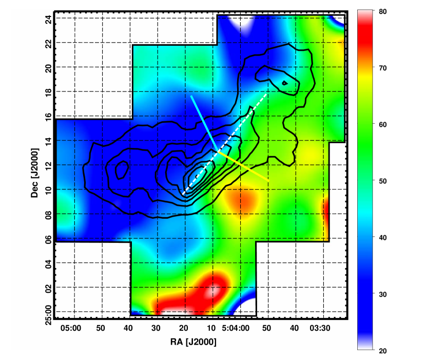
Figure 6: False-color map of mean $H$ band polarization position angle, PA (in degrees), across L1544, at 3 arcmin FWHM effective angular resolution. Color look-up wedge at right indicates mapping of PA (in deg) to displayed colors. Black contours show the Herschel  250 $\mu$m emission. The white, dashed line indicates the position angle of the cloud infrared emission ‘spine.’ The yellow, solid line shows the mean polarization PA South and West of the spine, and the cyan, solid line shows the mean polarization PA North and East of the spine. These indicate $B_{POS}$ orientations that are nearly perpendicular to the spine, but are also strongly changing at the position of the L1544 cloud spine.

One possible explanation is that the cloud ridge is located at a boundary, or collision, between two distinct magnetic media, with different $B_{POS}$ PAs. Another explanation is that the B-field changes close to the dust ridge because the B-field has significant helical pitch (Fiege & Pudritz, 2000) and manifests different $B_{POS}$ PAs on the two ‘sides’ of the cloud ridge.

3.1.6 Gas Kinematics and B-fields

The steep PA gradient associated with the elongated gas and dust ridge in L1544 might be expected to be associated with a similar gradient in the radial velocity of the gas, possibly generated through rotation of the L1544 cloud or envelope. Interestingly, while some velocity gradients have been detected in spectroscopic maps of various gas tracers, there is no clear indication of rotation.

A velocity gradient, mostly along the major axis of the cloud complex, is present when comparing the radial velocity of L1544-W (10 arcmin offset), L1544, and L1544-E (5 arcmin offset). Heyer et al. (1987) found an offset of about 0.4 km s^-1 across 37-40 arcmin in ¹³CO, yielding a gradient of 0.3 km s^-1 pc^-1. Similarly, Tafalla et al. (1998) used C¹⁸O to reveal a somewhat larger gradient of 1.1 km s^-1 pc^-1 along the major axis. Their channel maps also reveal that the L1544 core exhibits another velocity gradient, of about 3.4 km s^-1 pc^-1, along the decl direction. Using N₂H⁺, Williams et al. (1999), Caselli et al. (2002c), and Williams et al. (2006) found core velocity gradients of 3.8. 1.0, and 4.1 km s^-1 pc^-1, respectively, with the latter two value mostly along the decl axis.

However, neither the large-scale velocity gradient along the major cloud axis nor the smaller scale decl velocity gradient across the L1544 core exhibit a strong correlation with the polarization PA gradient shown in Figure 6. It may be that a weak shear due to the large-scale velocity gradient is bending the plane of sky B-field lines from PA 60$\arcdeg$  to PA 30$\arcdeg$  at the location of the cloud’s major axis, but why this would affect BSP PAs only on one side of the cloud (W) and not the other is unclear. There appears to be no evidence of strong cloud or core rotation and neither of the observed weak velocity gradients appears to explain the BSP PA change across L1544.

3.2 SCUBA 850 $\mu$m Dust Emission Polarization in the L1544 Core

The SCUPOL instrument combination was used on the JCMT by Ward-Thompson et al. (2000) to probe the L1544 core for linear polarization of the thermal dust emission at 850 $\mu$m. These data were also used by Crutcher et al. (2004) to estimate the $B_{POS}$ field strength in the core, using the C-F method. Matthews et al. (2009) reprocessed all SCUPOL data taken on the JCMT to produce an improved and uniformly calibrated legacy data archive. This included refined gain calibration for all pixels and yielded improved maps of Stokes $I$, $Q$, $U$, and their uncertainties. These reprocessed SCUPOL data for L1544 were obtained from the legacy archive and post-processed for this current study using techniques similar to those described above.

The polarization SNRs at the native $10\times 10$ arcsec pixel sizes (the diffraction-limited beam size was 14 arcsec) in the archive data are too low to yield adequate constraints on the polarization position angles for more than a couple of positions. This relates to the small number of positions (8) showing $P$ SNR$>2$ selected by Ward-Thompson et al. (2000) for plotting and used by Crutcher et al. (2004) for C-F method analysis. But, post-processing options are available which utilize more of the submm information and can increase the number of independent positions with detectable submm polarization. Here, to boost the SNR (though at the expense of angular resolution), the Stokes $Q$ and $U$ maps from the archive were smoothed, using weighting by both the archive $Q$ and $U$ variance maps and a gaussian taper, of FWHM 35 arcsec, and resampled onto 25 arcsec pixels. From these smoothed Stokes parameter maps, maps of $P$ and its uncertainty $\sigma_{P}$ were developed and debiased to yield $P^{\prime}$ values. A mask image was generated which selected all (smoothed, resampled) map pixels having $P^{\prime}/\sigma_{P}\geq 1.9$, corresponding to $\sigma_{PA}\leq 15\arcdeg$, and which had Stokes $I$ values more than 25% of the peak, smoothed value. A polarization PA map was computed from the smoothed Stokes maps, masked, and the PA values were rotated by 90$\arcdeg$  to represent $B_{POS}$ orientations.

Figure 7 displays the twenty map pixels that passed the mask operation, with $B_{POS}$ PA values coded into the color of each 25 arcsec pixel and the orientations of the black line segments. The yellow contours show the Stokes $I$ distribution for the 850 $\mu$m dust emission. The pixel $P^{\prime}$ and $B_{POS}$ PA values are listed in Table 2. The variance-weighted mean PA of all 20 points is $9.9\pm 1.6\arcdeg$  and the $\Delta_{PA}$(raw) is 20.4$\arcdeg$. Following Crutcher et al. (2004), $\Delta_{PA}$(raw) was debiased by the mean $\sigma_{PA}=8.3\arcdeg$  to yield $\Delta_{PA}$(corrected) of 18.6$\arcdeg$. This value is larger than found by Crutcher et al. (2004) for the eight positions reported by Ward-Thompson et al. (2000) for the SCUPOL data, but prior to the Matthews et al. (2009) reprocessing.

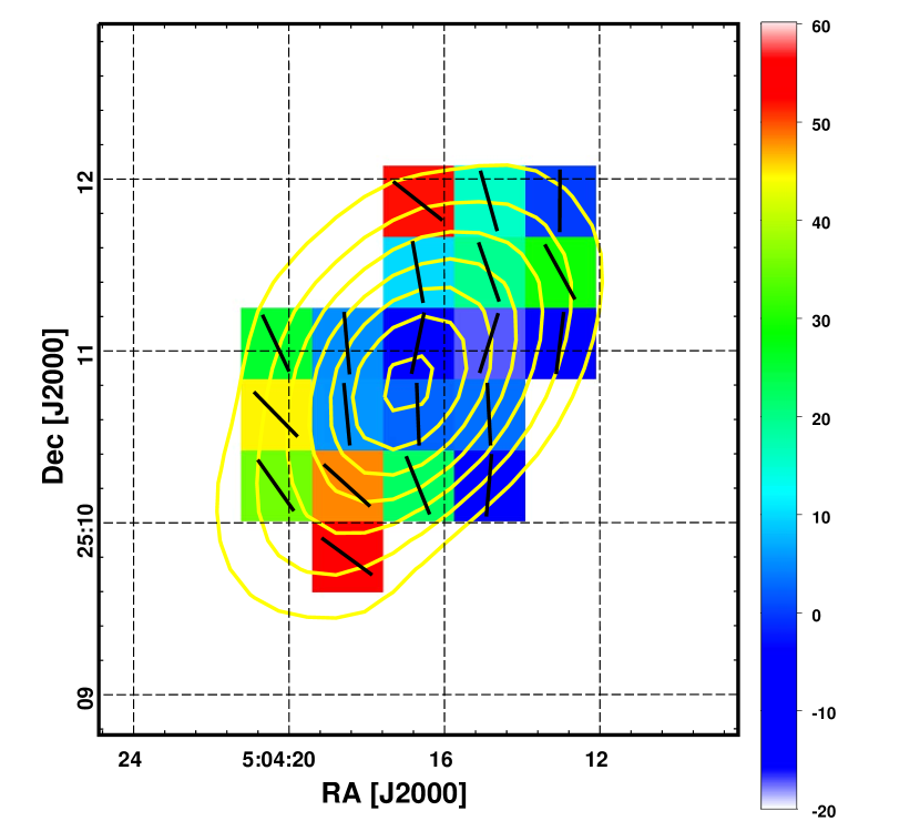
Figure 7: False-color and black vector representations of the $B_{POS}$ PA (in degrees and rotated 90$\arcdeg$  from the dust emission electric field polarization PA) measured by SCUPOL at 850 $\mu$m, after smoothing the Stokes parameters maps to 35 arcsec FWHM and sampling on a 25 arcsec grid. Color look up table at right shows how colors map to PA (in deg). Pixels shown have $\sigma_{PA}\leq 15\arcdeg$. Yellow contours show Stokes $I$ surface brightness at 850 $\mu$m, starting at 43 kJy sr^-1 and increasing in steps of half of that value.

Table 2: SCUPOL 850 $\mu$m Polarizations

Pixel	RA	decl.	$P^{\prime}$	$B_{POS}$ PA
	[$\arcdeg$]	[$\arcdeg$]	[%]	[$\arcdeg$]
1	76.05390	25.18405	3.80 (1.21)	173.1 (9.1)
2	76.05390	25.19095	3.70 (1.20)	28.8 (9.3)
3	76.05390	25.19785	4.70 (1.92)	179.7 (11.8)
4	76.06152	25.17026	9.72 (1.56)	175.2 (4.6)
5	76.06152	25.17716	2.97 (0.74)	3.0 (7.1)
6	76.06152	25.18405	2.52 (0.61)	162.6 (7.0)
7	76.06152	25.19095	3.07 (0.75)	19.2 (7.0)
8	76.06152	25.19785	5.95 (1.38)	15.6 (6.6)
9	76.06914	25.17026	2.24 (0.75)	22.0 (9.5)
10	76.06914	25.17716	2.04 (0.45)	2.24 (6.3)
11	76.06914	25.18405	3.30 (0.46)	168.3 (4.0)
12	76.06914	25.19095	1.36 (0.70)	9.8 (14.8)
13	76.06914	25.19785	4.78 (1.53)	51.8 (9.2)
14	76.07676	25.16337	3.61 (1.15)	53.8 (9.1)
15	76.07676	25.17026	3.27 (0.73)	48.0 (6.4)
16	76.07676	25.17716	2.09 (0.54)	5.4 (7.4)
17	76.07676	25.18405	3.60 (0.66)	5.0 (5.3)
18	76.08438	25.17026	2.33 (1.16)	35.2 (14.3)
19	76.08438	25.17716	3.09 (1.18)	44.5 (11.0)
20	76.08438	25.18405	6.88 (1.43)	25.2 (6.0)

However, examination of Figure 7 reveals that the Matthews et al. (2009) reprocessing plus post-processing reveals complexity not seen in the older works. The Figure shows that the vectors closest to the intensity peak have a nearly vertical, PA=0$\arcdeg$, orientation while the vectors farther from the peak have PAs closer to 30-40$\arcdeg$. This distinction can be seen post-facto in the Ward-Thompson et al. (2000) map, though the number of central pixels is only two or three, and the number of outer pixels is similarly small. The impression from the reprocessed data is that the central $B_{POS}$ orientation is closer to being parallel to the major axis of the L1544 dense core dust structure, while the outer regions show $B_{POS}$ orientations more in agreement with the NIR values. Indeed, if the eight new positions located closest to the intensity peak are considered as a subset, their mean $B_{POS}$ PA is $177.4\pm 2.2\arcdeg$ and their $\Delta_{PA}$(corrected) is 15.9$\arcdeg$, compared to PA$=22.5\pm 2.2\arcdeg$ and $\Delta_{PA}$(corrected) of 23.9$\arcdeg$ for the twelve positions surrounding the core. The mean PAs for the two subsets differ by 8$\sigma$, indicating significant $B_{POS}$ changes within the Arecibo Zeeman beam size.

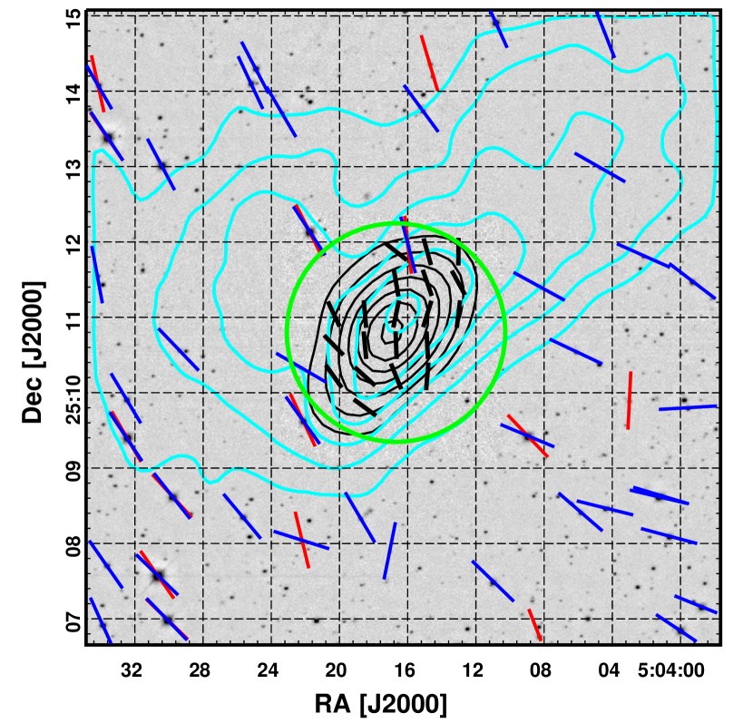
Figure 8: Grayscale Mimir deep $H$-band image, zoomed to show the central $8\times 8$ arcmin region including the L1544 dense cloud core. Mimir $H$-band polarization vectors are displayed as blue line segments, with all segment lengths set equal to highlight B-field orientations. Mimir $K$-band polarization vectors are similarly shown as red line segments. Black vectors are the SCUPOL values seen in the previous Figure. Cyan contours show the Herschel  250 $\mu$m dust emission. Black contours show JCMT/SCUBA Stokes $I$ from the previous Figure. The green circle is the Arecibo FWHM beam size for the Crutcher et al. (2009) observations.

A comparison between reprocessed SCUPOL and NIR BSP $B_{POS}$ PA values is shown in Figure 8. This $8\times 8$ arcmin Mimir survey region center shows $H$ band PA vectors in blue, $K$ band PA vectors in red, and (90$\arcdeg$  rotated) SCUPOL vectors in black. Together, they reveal a twist in $B_{POS}$ orientations in going from the dense core out to the larger, lower density region that starts approximately at the Arecibo beamsize circle, where the SCUPOL vectors begin to match the NIR vectors.

4 Discussion

4.1 NIR BSP Traces B-fields in L1544

The evidence presented above shows that the L1544 cloud, as revealed in the Herschel 250 $\mu$m thermal dust emission (Figure 1), is well-traced by NIR reddening using the RJCE $E(H-M)$ colors (Figure 2). That same dust is responsible for both BSP in the NIR (Figure 3 and Figure 4) as well as thermal emission polarization in the submm (Figure 7).

The changes in the polarization properties with direction on the sky, especially changes in the mean PA orientation (Figure 6) and changes in $\Delta_{PA}$ (Figure 5), correlate strongly with location relative to the ‘spine’ of the L1544 cloud and its dense core. That the PAs change so dramatically at the location of the cloud and yet $\Delta_{PA}$ reaches its lowest minimum there argue for close coupling of the B-field and the gas and dust within L1544.

The strong decrease in the NIR $\Delta_{PA}$ associated with the cloud spine and in the core, and the overall outer-core agreement of the NIR and SCUBA B-field orientations (Figure 8), points to increases in the B-field strength with gas density in L1544. To quantify this increase, and indeed to perform a close comparison of $B_{POS}$ to $B_{LOS}$ (radio Zeeman) amplitudes, requires establishing the mean gas density and velocity dispersion across the NIR survey zone and invocation of the C-F method. These are outside the scope of this current paper, but are the subjects of later papers in this series.

4.2 The Non-Uniform B-Field in the L1544 Cloud Envelope

The Crutcher et al. (2009) analysis of the Zeeman properties of their clouds’ envelopes assumed that each of the GBT pointings sampled the same, uniform regular B-field and thus measured a single, representative value of $B_{LOS}$ for each cloud envelope. Assessing the validity of this assumption requires examining whether the GBT beams covered regions of similar or non-similar B-fields for each cloud. No quantitative measure of B-field uniformity exists to easily address when B-fields are uniform enough to return unbiased results when samples are averaged as per Crutcher et al. (2009). Instead, a statistical assessment of key polarization properties was performed for L1544 using the $B_{POS}$ NIR BSP data of Table 1.

For each of the Arecibo and GBT beams, the $H$ band, $K$ band, and SCUPOL data sets were sampled. A suitable gaussian taper was computed for each star or SCUBA position, with respect to the center of each Arecibo or GBT beam, with each gaussian taper FWHM width set to the corresponding beamsize FWHM width. Additional weighting was by the variance of the quantity being ‘observed’ using these synthetic beams. The data were selected to be of good quality, by applying $P^{\prime}$ and PA uncertainty cuts ($\sigma_{P}<$ 3%; $\sigma_{PA}<45\arcdeg$). Very low uncertainties (associated with the brightest stars) were trapped to be no less than the lowest quartile uncertainties to prevent a few values from dominating the weighted means.

Most of the stellar values used were $H$-band based, which yielded 329 entries after applying the criteria above. Similarly, $K$ band provided 29 stars and SCUPOL provided all 20 positions. The means and uncertainties for polarization PA, $\Delta_{PA}$, and $P^{\prime}$ were computed for the different combination of $H$ band and $K$ band samples, as well as $H$+$K$ bands, SCUPOL, and SCUPOL+$H$+$K$ sample combinations. Note that SCUPOL points cover only the central, Arecibo beam.

Figure 9 shows, and Table 3 lists, the beam-based comparisons of plane-of-sky means of PA, $\Delta_{PA}$, and $P^{\prime}$ values. In the Figure, the $x$-axis displays ‘Orientation PA,’ which was defined as the projected PA from the Arecibo beam center to each of the regions covered by a GBT beam (with the usual East-from-North angle increment). Thus, the ‘GBT-N’ (North) beam is centered at Orientation PA=0$\arcdeg$, but spans about $\pm 40\arcdeg$  of Orientation PA. In this plot, a uniform B-field in the envelope of L1544 would show the same polarization PA (or other property) for all Orientation PAs. The Table presents the NIR weighted means and uncertainties, using $H$ and $K$ band stellar data for PA and $\Delta_{PA}$ and $H$ band data alone for $P^{\prime}$. For the Arecibo beam average, the first line in the Table presents the $H$ and $K$ values, while the second line includes the effects of the (weighted) SCUPOL points.

In the top panel of Figure 9, the red points show the polarization PA averages and uncertainties as well as the effective widths of the GBT beams in Orientation PA. The numbers below each GBT beam identifier list the effective number of stars used in the H and K band averages. These are effective numbers because of the gaussian tapers - all of the individual stars contribute, but only in summed gaussian weights equivalent to the listed numbers. The violet line and hatching show the same polarization PA and uncertainty for the H and K stars in the Arecibo beam (much smaller than the GBT beams and centered on the opaque cloud core). The blue line and hatching add the SCUPOL values to the H and K ones. The Orientation PA of the Arecibo beam spans 0-360$\arcdeg$, hence the use of the hatched regions to render its values.

This panel displays just how different the polarization properties are in the different GBT and Effelsberg beams. While the polarization PAs of two of the beams (GTB-N and GBT-E) are partially consistent with each other (differing by 5$\sigma$) and also with one, or the other, Arecibo beam estimate, the other two beams’ polarization PAs are quite different (6.5 sigma for GBT-S and 23 sigma for GBT-W, both compared to GBT-N). These position-to-position differences indicate that the B-field is unlikely to be uniform in the envelope surrounding the L1544 core.

The middle panel is the same type of comparison for $\Delta_{PA}$ values. The differences, compared to the values for the central Arecibo beam, are less significant here, though large differences between the values in the GBT beams remain. This is especially true when comparing the GBT-N and -E beam values to the GBT-S and -W beam values.

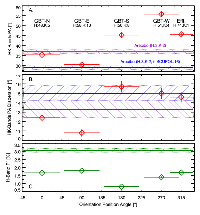
Figure 9: Comparison of $H$, $K$, and SCUPOL polarizations in the Crutcher et al. (2009) Arecibo and GBT beams (as well as in the Effelsberg beam). Horizontal axis is Orientation PA of the GBT beams, seen from Arecibo beam center. Red and green diamonds with error bars are beam-averaged values, uncertainties, and Orientation PAs. Top, A, panel shows polarization PA, from $H$ and $K$. Beam designations and effective stellar numbers by band (see text) run along panel top. PAs for Arecibo are violet horizontal line and hatching for $H$ and $K$, and blue line and hatching when also including SCUPOL data. Middle, B, panel compares $\Delta_{PA}$. Bottom, C, panel compares $H$-band $P^{\prime}$, with Arecibo value and uncertainty as the green line and hatching. Strong beam-to-beam variations in PA and $P^{\prime}$ and weaker variations in $\Delta_{PA}$ indicate $B_{POS}$ is unlikely to be highly uniform in the GBT-sampled L1544 envelope.

Table 3: NIR BSP Properties in Arecibo, GBT, and Effelsberg Beams

Region	Orientation PA	$<P^{\prime}_{H}>$	$<PA>$	$\sigma_{PA}$
	[$\arcdeg$]	[%]	[$\arcdeg$]	[$\arcdeg$]
(1)	(2)	(3)	(4)	(5)
Arecibo - Dense Core - HK only	…	3.06 (0.11)	36.9 (1.0)	13.3 (0.9)
Arecibo - HK+SCUPOL	…	…	29.0 (0.8)	15.0 (0.8)
GBT - North	$-$40 - $+$40	1.66 (0.04)	35.4 (0.7)	12.4 (0.5)
GBT - East	50 - 130	1.80 (0.04)	30.5 (0.6)	10.8 (0.4)
GBT - South	140 - 220	0.80 (0.04)	45.3 (1.3)	15.7 (0.6)
GBT - West	230 - 310	1.39 (0.05)	55.8 (0.9)	15.0 (0.6)
Effelsberg - NW	289 - 341	1.68 (0.05)	45.7 (0.8)	14.6 (0.5)

The bottom panel compares $P^{\prime}$ values for $H$ band, only, as no other similar comparison covers all of the beams. The GBT beams would not be expected to contain background stars exhibiting polarizations as high as those seen in the Arecibo beam, but a uniform B-field in the L1544 envelope might be expected to yield better uniformity of $P^{\prime}$ across the GBT beams. This is not what is seen here: the GBT-N and GBT-S beams show $P^{\prime}$ values that differ by 15$\sigma$.

The statistically different PA orientations and dispersions in the L1544 envelope-tracing GBT beams, and indeed the PA twist newly uncovered in the SCUPOL data within the Arecibo beam, suggest that simple averaging of Zeeman detections (especially with non-detections) for the purpose of estimating relative core-envelope $M/\Phi$ values by Crutcher et al. (2009) is likely to be biased. Detailed conclusions regarding the applicability of AD models to dense core formation and evolution, which rest on relative core/envelope $M/\Phi$ estimates, must be revisited using more robust observational approaches, including deeper analyses of the current NIR BSP data.

5 Summary

Accurately characterizing B-fields is challenging, but is vital to understanding how molecular clouds form, evolve, and produce new stars. Testing leading B-field models that address these phases is equally important, and must be performed using a variety of techniques and tools. Here, new near-infrared imaging stellar background polarimetry, and post-processing of the archived re-reduced SCUPOL data, were used to survey the full extent of the L1544 dark cloud, which has the best radio OH Zeeman effect detections (of its core and one envelope position) of any dark cloud.

The first goal of this study was to show that near-infrared starlight polarimetry is able to reveal B-fields across the L1544 cloud at high angular sampling and precision. This goal was met by revealing that the positional changes in plane-of-sky B-field PA orientations and dispersions of those orientations correlate strongly with the location and structure of the L1544 dust thermal emission.

The second goal was to test whether the plane-of-sky polarization properties were uniform throughout the envelope of L1544 or whether these properties vary significantly. A key assumption of the analysis of OH Zeeman observations, performed by Crutcher et al. (2009) and leading to relative mass-to-flux ratios of the L1544 core and envelope, was that the B-field was uniform in the envelope, permitting averaging of the Zeeman observations across the four GBT beam pointings without accounting for possible beam-to-beam intrinsic variations.

The near-infrared background starlight polarimetry, averaged over each of the different GBT Zeeman beam sizes and positions observed, instead showed strong beam-to-beam variations in the plane-of-sky polarization properties. The reprocessed SCUPOL data showed a similar strong change in PA directions within the much smaller Arecibo beamsize used for the initial Zeeman detection of the core B-field.

Averaging low-signal Zeeman observations from different pointings without treating intrinsic variations would be effective if the B-field were uniform across the pointings. For L1544, the near-infrared polarimetry results are at odds with this uniformity assumption and thereby the conclusions that rest upon it.

References

- Arce et al. (1998) Arce, H. G., Goodman, A. A., Bastien, P., Manset, N., & Sumner, M. 1998, ApJ, 499, L93
- Bacmann et al. (2000) Bacmann, A., André, P., Puget, J.-L., et al. 2000, A&A, 361, 555
- Basu & Mouschovias (1994) Basu, S., & Mouschovias, T. Ch. 1994, ApJ, 432, 720
- Benson et al. (1998) Benson, P. J., Caselli, P., & Myers, P. C. 1998, ApJ, 506, 743
- Bizzocchi et al. (2014) Bizzocchi, L., Caselli, P., Spezzano, S., & Leonardo, E. 2014, A&A, 569, A27
- Caselli et al. (2002a) Caselli, P., Walmsley, C. M., Zucconi, A., et al. 2002a, ApJ, 565, 331
- Caselli et al. (2002b) Caselli, P., Walmsley, C. M., Zucconi, A., et al. 2002b, ApJ, 565, 344
- Caselli et al. (2002c) Caselli, P., Benson, P. J., Myers, P. C., & Tafalla, M. 2002c, ApJ, 572, 238
- Caselli et al. (2010) Caselli, P., Keto, E., Pagani, L., et al. 2010, A&A, 521, L29
- Chandrasekhar & Fermi (1953) Chandrasekhar, S., & Fermi, E. 1953, ApJ, 118, 113
- Ciolek & Mouschovias (1994) Ciolek, G. E., & Mouschovias, T. Ch. 1994, ApJ, 425, 142
- Ciolek & Basu (2000) Ciolek, G. E., & Basu, S. 2000, ApJ, 529, 925
- Clemens et al. (2007) Clemens, D. P., Sarcia, D., Grabau, A., et al. 2007, PASP, 119, 1385
- Clemens et al. (2012c) Clemens, D. P., Pavel, M. D., & Cashman, L. R. 2012c, ApJS, 200, 21
- Clemens et al. (2012b) Clemens, D. P., Pinnick, A. F., & Pavel, M. D. 2012b, ApJS, 200, 20
- Clemens et al. (2012a) Clemens, D. P., Pinnick, A. F., Pavel, M. D., & Taylor, B. W. 2012a, ApJS, 200, 19
- Crapsi et al. (2005) Crapsi, A., Caselli, P., Walmsley, C. M., et al. 2005, ApJ, 619, 379
- Crutcher (1999) Crutcher, R. M. 1999, ApJ, 520, 706
- Crutcher (2012) Crutcher, R. M. 2012, ARA&A, 50, 29
- Crutcher et al. (1996) Crutcher, R. M., Troland, T. H., Lazareff, B., & Kazes, I. 1996, ApJ, 456, 217
- Crutcher et al. (2009) Crutcher, R. M., Hakobkian, N., & Troland, T. H. 2009, ApJ, 692, 844
- Crutcher & Troland (2000) Crutcher, R. M., & Troland, T. H. 2000, ApJ, 537, L139
- Crutcher et al. (2004) Crutcher, R. M., Nutter, D. J., Ward-Thompson, D., & Kirk, J. M. 2004, ApJ, 600, 279
- Cutri et al. (2003) Cutri, R. M., Skrutskie, M. F., van Dyk, S., et al. 2003, VizieR Online Data Catalog, 2246, 0
- Cutri et al. (2013) Cutri, R. M., & et al. 2013, VizieR Online Data Catalog, 2328, 0
- Doty et al. (2005) Doty, S. D., Everett, S. E., Shirley, Y. L., Evans, N. J., & Palotti, M. L. 2005, MNRAS, 359, 228
- Elias (1978) Elias, J. H. 1978, ApJ, 224, 857
- Fiedler & Mouschovias (1992) Fiedler, R. A., & Mouschovias, T. Ch. 1992, ApJ, 391, 199
- Fiege & Pudritz (2000) Fiege, J. D., & Pudritz, R. E. 2000, MNRAS, 311, 85
- Galli & Shu (1993) Galli, D., & Shu, F. H. 1993, ApJ, 417, 220
- Girart et al. (1999) Girart, J. M., Crutcher, R. M., & Rao, R. 1999, ApJ, 525, L109
- Goldreich & Kylafis (1981) Goldreich, P., & Kylafis, N. D. 1981, ApJ, 243, L75
- Goodman et al. (1989) Goodman, A. A., Crutcher, R. M., Heiles, C., Myers, P. C., & Troland, T. H. 1989, ApJ, 338, L61
- Goodman et al. (1995) Goodman, A. A., Jones, T. J., Lada, E. A., & Myers, P. C. 1995, ApJ, 448, 748
- Greaves et al. (2003) Greaves, J. S., Holland, W. S., Jenness, T., et al. 2003, MNRAS, 340, 353
- Hennebelle & Fromang (2008) Hennebelle, P., & Fromang, S. 2008, A&A, 477, 9
- Heyer et al. (1987) Heyer, M. H., Vrba, F. J., Snell, R. L., et al. 1987, ApJ, 321, 855
- Holland et al. (1999) Holland, W. S., Robson, E. I., Gear, W. K., et al. 1999, MNRAS, 303, 659
- Jones et al. (2015) Jones, T. J., Bagley, M., Krejny, M., Andersson, B.-G., & Bastien, P. 2015, AJ, 149, 31
- Joye & Mandel (2003) Joye, W. A., & Mandel, E. 2003, in Astronomical Data Analysis Software and Systems XII, H. E. Payne, R. I. Jedrzejewski, & R. N. Hook, eds., ASP Conf. Ser., 295, 489
- Kenyon et al. (1994) Kenyon, S. J., Dobrzycka, D., & Hartmann, L. 1994, AJ, 108, 1872
- Keto & Caselli (2008) Keto, E., & Caselli, P. 2008, ApJ, 683, 238
- Keto & Caselli (2010) Keto, E., & Caselli, P. 2010, MNRAS, 402, 1625
- Keto et al. (2014) Keto, E., Rawlings, J., & Caselli, P. 2014, MNRAS, 440, 2616
- Keto et al. (2015) Keto, E., Caselli, P., & Rawlings, J. 2015, MNRAS, 446, 3731
- Lee et al. (2003) Lee, J.-E., Evans, N. J., II, Shirley, Y. L., & Tatematsu, K. 2003, ApJ, 583, 789
- Li et al. (2014) Li, H.-B., Goodman, A., Sridharan, T. K., et al. 2014, Protostars and Planets VI, 101
- Li et al. (2015) Li, P. S., McKee, C. F., & Klein, R. I. 2015, MNRAS, 452, 2500
- Li & Nakamura (2002) Li, Z.-Y., & Nakamura, F. 2002, ApJ, 578, 256
- Li et al. (2002) Li, Z.-Y., Shematovich, V. I., Wiebe, D. S., & Shustov, B. M. 2002, ApJ, 569, 792
- Majewski et al. (2011) Majewski, S. R., Zasowski, G., & Nidever, D. L. 2011, ApJ, 739, 25
- Matthews et al. (2009) Matthews, B. C., McPhee, C. A., Fissel, L. M., & Curran, R. L. 2009, ApJS, 182, 143
- Messinger et al. (1997) Messinger, D. W., Whittet, D. C. B., & Roberge, W. G. 1997, ApJ, 487, 314
- Mestel & Spitzer (1956) Mestel, L., & Spitzer, L., Jr. 1956, MNRAS, 116, 503
- Mouschovias (1976a) Mouschovias, T. Ch. 1976a, ApJ, 206, 753
- Mouschovias (1976b) Mouschovias, T. Ch. 1976b, ApJ, 207, 141
- Mouschovias (1996a) Mouschovias, T. Ch. 1996a, NATO Advanced Science Institutes (ASI) Series C, 481, 475
- Mouschovias (1996b) Mouschovias, T. Ch. 1996b, NATO Advanced Science Institutes (ASI) Series C, 481, 505
- Mouschovias (1991) Mouschovias, T. Ch. 1991, ApJ, 373, 169
- Mouschovias et al. (2006) Mouschovias, T. Ch., Tassis, K., & Kunz, M. W. 2006, ApJ, 646, 1043
- Mouschovias & Tassis (2010) Mouschovias, T. Ch., & Tassis, K. 2010, MNRAS, 409, 801
- Myers et al. (1983) Myers, P. C., Linke, R. A., & Benson, P. J. 1983, ApJ, 264, 517
- Myers & Benson (1983) Myers, P. C., & Benson, P. J. 1983, ApJ, 266, 309
- Padoan & Nordlund (1999) Padoan, P., & Nordlund, Å. 1999, ApJ, 526, 279
- Pillai et al. (2015) Pillai, T., Kauffmann, J., Tan, J. C., et al. 2015, ApJ, 799, 74
- Serkowski et al. (1975) Serkowski, K., Mathewson, D.S., & Ford, V.L. 1975, ApJ, 196, 261
- Shirley et al. (2000) Shirley, Y. L., Evans, N. J., II, Rawlings, J. M. C., & Gregersen, E. M. 2000, ApJS, 131, 249
- Skrutskie et al. (2006) Skrutskie, M.F., Cutri, R. M., Stiening, R., et al. 2006, AJ, 131, 1163.
- Snell (1981) Snell, R. L. 1981, ApJS, 45, 121
- Tafalla et al. (1998) Tafalla, M., Mardones, D., Myers, P. C., et al. 1998, ApJ, 504, 900
- Tafalla et al. (2002) Tafalla, M., Myers, P. C., Caselli, P., Walmsley, C. M., & Comito, C. 2002, ApJ, 569, 815
- Torres et al. (2012) Torres, R. M., Loinard, L., Mioduszewski, A. J., et al. 2012, ApJ, 747, 18
- Troland & Crutcher (2008) Troland, T. H., & Crutcher, R. M. 2008, ApJ, 680, 457
- van der Tak et al. (2005) van der Tak, F. F. S., Caselli, P., & Ceccarelli, C. 2005, A&A, 439, 195
- Vastel et al. (2006) Vastel, C., Caselli, P., Ceccarelli, C., et al. 2006, ApJ, 645, 1198
- Ward-Thompson et al. (1999) Ward-Thompson, D., Motte, F., & Andre, P. 1999, MNRAS, 305, 143
- Ward-Thompson et al. (2000) Ward-Thompson, D., Kirk, J. M., Crutcher, R. M., et al. 2000, ApJ, 537, L135
- Wardle & Kronberg (1974) Wardle, J. F. C., & Kronberg, P. P. 1974, ApJ, 194, 249
- Whittet et al. (2008) Whittet, D. C. B., Hough, J. H., Lazarian, A., & Hoang, T. 2008, ApJ, 674, 304
- Wilking et al. (1980) Wilking, B. A., Lebofsky, M. J., Kemp, J. C., et al. 1980, ApJ, 235, 905
- Williams et al. (1999) Williams, J. P., Myers, P. C., Wilner, D. J., & Di Francesco, J. 1999, ApJ, 513, L61
- Williams et al. (2006) Williams, J. P., Lee, C. W., & Myers, P. C. 2006, ApJ, 636, 952
- Wright et al. (2010) Wright, E. L., Eisenhardt, P. R. M., Mainzer, A. K., et al. 2010, AJ, 140, 1868
- Zacharias et al. (2010) Zacharias, N., Finch, C., Girard, T., et al. 2010, AJ, 139, 2184
- Zhang et al. (2014) Zhang, Q., Qiu, K., Girart, J. M., et al. 2014, ApJ, 792, 116