A note on exponential Rosenbrock-Euler method for the finite element discretization of a semilinear parabolic partial differential equation

Abstract

In this paper, we consider the numerical approximation of a general second order semi–linear parabolic partial differential equation. Equations of this type arise in many contexts, such as transport in porous media. Using finite element method for space discretization and the exponential Rosenbrock-Euler method for time discretization, we provide a convergence proof in space and time under only the standard Lipschitz condition of the nonlinear part, for both smooth and nonsmooth initial solution. This is in contrast to restrictive assumptions made in the literature, where the authors have considered only approximation in time so far in their convergence proofs. The main result reveals how the convergence orders in both space and time depend heavily on the regularity of the initial data. In particular, the method achieves optimal convergence order $\mathcal{O}\left(h^{2}+\Delta t^{2}t_{m}^{-\eta}\right)$ when the initial data belongs to the domain of the linear operator. Numerical simulations to sustain our theoretical result are provided.

1 Introduction

We consider the following abstract Cauchy problem with boundary conditions

$$\dfrac{du(t)}{dt}=Au(t)+F(u(t)),\quad u(0)=u_{0},\quad t\in(0,T],\quad T>0,$$ (1)

on the Hilbert space $H=L^{2}(\Lambda)$, where $\Lambda$ is an open subset of $\mathbb{R}^{d}$ $(d=1,2,3)$, which is supposed to be a convex polygon or has a smooth boundary. The linear operator $A:\mathcal{D}(A)\subset H\longrightarrow H$ is negative, not necessarily self adjoint and generates an analytic semigroup $S(t):=e^{At}$, $t\geq 0$. Without loss of generality, the nonlinear function $F:H\longrightarrow H$ is assumed to be autonomous. Our main focus will be on the case where $A$ is a general second order elliptic operator. Under some technical conditions (see e.g. [10, 28]), it is well known that the mild solution of (1) is given by

$$u(t)=S(t)u_{0}+\int_{0}^{t}S(t-s)F\left(u(s)\right)ds,\quad t\in[0,T].$$ (2)

In general, it is hard to find the exact solutions of many PDEs. Numerical approximations are currently the only important tools to approximate the solutions. Approximations are done at two levels, spatial approximation and temporal approximation. The finite element [35], finite volume [32], finite difference methods are mostly used for space discretization of the problem (1), while explicit, semi implicit and fully implicit methods are usually used for time discretization. References about standard discretization methods for (1) can be found in [32]. Due to the time step size constraints, fully implicit schemes are more popular for the time discretization for quite a long time compared to explicit Euler schemes. However, implicit schemes need at each time step a solution of large systems of nonlinear equations. This can be the bottleneck in computations when dealing with realistic problems. Recent years, exponential integrators have become an attractive alternative in many evolutions equations [3, 11, 12, 27, 32, 33]. Most exponential integrators analyzed early in the literature [3, 12, 27] were bounded on the nonlinear problem as in (1) where the linear part $A$ and the nonlinear function $F$ are explicitly known a priori. Such approach is justified in situations where the nonlinear function $F$ is small. Due to the fact that in more realistic applications the nonlinear function $F$ can be stronger, Exponential Rosenbrock-Type methods have been proposed in [2, 13], where at every time step, the Jacobian of $F$ is added to the linear operator $A$. The lower order of them, called Exponential Rosenbrock-Euler method (EREM) has been proved to be efficient in various applications [8, 33]. For smooth initial solutions, this method is well known to be second order convergence in time [2, 13] and have good stability properties in the stochastic context [24]. However in many applications initial solutions are not always smooth. Typical examples are option pricing in finance or reaction diffusion advection with discontinuous initial solution. We refer to [6, 9, 14, 18, 21, 25, 26] for standard numerical technique with nonsmooth initial data. Recently exponential Rosenbrock-Euler with nonsmooth initial solution was analysed in [30, 31] under the additional hypothesis [30, 31, Assumption 1]. Furthermore, to the best of our knowledge, only convergence in time is investigated for smooth or nonsmooth initial solution in all existing Exponential Rosenbrock-Type methods.

The goal of this paper is to provide a rigorous convergence proof of EREM in space and time for both smooth and nonsmooth initial solution under more relaxed conditions than those used in [30, 31]. Indeed only the standard Lipschitz condition of the nonlinear part is used in our convergence analysis and optimal convergence orders in space and time are achieved. In fact the method achieves convergence orders of $\mathcal{O}\left(h^{\beta}+\Delta t^{1+\beta/2}t_{m}^{-\eta}\right)$, where $\beta$ is the regularity parameter of the initial data (see Assumption 2.1) and $\eta$ the parameter defined in Assumption 2.2. Note that when dealing with space discretization, more novel and careful estimates need to be derived. This is because the constant appearing in the error estimate should not depend on the space discretization parameter $h$. The space discretization is performed using finite element method. Recent work in [32] can be used to obtain the similar convergence proof for finite volume method.

The paper is organized as follows. In Section 2, result about the well posedness are provided along with EREM scheme and the main result. The proof of the main result is presented in Section 3. In Section 4, we present some numerical simulations to sustain our theoretical result.

2 Mathematical setting and numerical method

2.1 Notations, setting and well posedness

Let us start by presenting briefly notations, the main function spaces and norms that will be used in this paper. We denote by $\|\cdot\|$ the norm associated to the inner product $(\cdot,\cdot)$ of the Hilbert space $H=L^{2}(\Lambda)$. The norms in the Sobolev spaces $H^{m}(\Lambda),\,m\geqslant 0$ will be denoted by $\|.\|_{m}$. For a Hilbert space $U$ we denote by $\|\cdot\|_{U}$ the norm of $U$, $L(U,H)$ the set of bounded linear operators from $U$ to $H$. For ease of notation, we use $L(U,U)=:L(U)$. In the sequel, for convenience of presentation we take $A$ to be a second-order operator as this simplifies the convergence proof. More precisely, we assume $A$ to be given by

$$Au=\sum_{i,j=1}^{d}\dfrac{\partial}{\partial x_{i}}\left(q_{ij}(x)\dfrac{\partial u}{\partial x_{j}}\right)-\sum_{i=1}^{d}q_{i}(x)\dfrac{\partial u}{\partial x_{i}},$$ (3)

where $q_{ij}\in L^{\infty}(\Lambda)$, $q_{i}\in L^{\infty}(\Lambda)$. We assume that there is a constant $c_{1}>0$ such that

$$\sum_{i,j=1}^{d}q_{ij}(x)\xi_{i}\xi_{j}\geq c_{1}|\xi|^{2},\quad\xi\in\mathbb{R}^{d},\quad x\in\overline{\Omega}.$$ (4)

As in [7, 20], we introduce two spaces $\mathbb{H}$ and $V$, such that $\mathbb{H}\subset V$, that depend on the choice of the boundary conditions for the domain of the operator $A$ and the corresponding bilinear form. For example, for Dirichlet (or first-type) boundary conditions we take

$$V=\mathbb{H}=H^{1}_{0}(\Lambda)=\{v\in H^{1}(\Lambda):v=0\quad\text{on}\quad\partial\Lambda\}.$$ (5)

For Robin (third-type) boundary condition and Neumann (second-type) boundary condition, which is a special case of Robin boundary condition ($\alpha_{0}=0$), we take $V=H^{1}(\Lambda)$

$$\mathbb{H}=\{v\in H^{2}(\Lambda):\partial v/\partial v_{A}+\alpha_{0}v=0,\quad\text{on}\quad\partial\Lambda\},\quad\alpha_{0}\in\mathbb{R}.$$ (6)

Using Green’s formula and the boundary conditions, we obtain the corresponding bilinear form associated to $-A$, given by

$$a(u,v)=\int_{\Lambda}\left(\sum_{i,j=1}^{d}q_{ij}\dfrac{\partial u}{\partial x_{i}}\dfrac{\partial v}{\partial x_{j}}+\sum_{i=1}^{d}q_{i}\dfrac{\partial u}{\partial x_{i}}v\right)dx,\quad u,v\in V,$$ (7)

for Dirichlet and Neumann boundary conditions, and

$$a(u,v)=\int_{\Lambda}\left(\sum_{i,j=1}^{d}q_{ij}\dfrac{\partial u}{\partial x_{i}}\dfrac{\partial v}{\partial x_{j}}+\sum_{i=1}^{d}q_{i}\dfrac{\partial u}{\partial x_{i}}v\right)dx+\int_{\partial\Lambda}\alpha_{0}uvdx,\quad u,v\in V.$$ (8)

for Robin boundary conditions. Using Gårding’s inequality, it holds that there exist two positive constants $\lambda_{0}$ and $c_{0}$ such that

$$a(v,v)\geq\lambda_{0}\|v\|^{2}_{1}-c_{0}\|v\|^{2},\quad\forall v\in V.$$ (9)

By adding and subtracting $c_{0}u$ on the right hand side of (1), we obtain a new operator that we still call $A$ corresponding to the new bilinear form that we still call $a$ such that the following coercivity property holds

$$(-Av,v)=a(v,v)\geq\;\lambda_{0}\|v\|_{1}^{2},\;\;\;\;\;\forall v\in V.$$ (10)

Note that the expression of the nonlinear term $F$ has changed as we included the term $-c_{0}u$ in the new nonlinear term that we still denote by $F$. The coercivity property (10) implies that $A$ is sectorial on $L^{2}(\Lambda)$, i.e. there exist $C_{1}\geq 0$ and $\theta\in(\frac{1}{2}\pi,\pi)$ such that

$$\|(\lambda I-A)^{-1}\|_{L(L^{2}(\Lambda))}\leq\dfrac{C_{1}}{|\lambda|},\;\quad\quad\lambda\in S_{\theta},$$ (11)

where $S_{\theta}=\left\{\lambda\in\mathbb{C}:\lambda=\rho e^{i\phi},\;\rho>0,\;0\leq|\phi|\leq\theta\right\}$ (see e.g. [10, 18, 20]). Therefore $A$ is the infinitesimal generator of a bounded analytic semigroup $S(t)=e^{tA}$ on $L^{2}(\Lambda)$ such that

$$S(t)=e^{tA}=\dfrac{1}{2\pi i}\int_{\mathcal{C}}e^{t\lambda}(\lambda I-A)^{-1}d\lambda,\;\;\;\;\;\;\;\;t>0,$$ (12)

where $\mathcal{C}$ denotes a path that surrounds the spectrum of $A$. The coercivity property (10) also implies that $-A$ is a positive operator and its fractional powers are well defined for any $\alpha>0,$ by

$$\left\{\begin{array}[]{rcl}(-A)^{-\alpha}&=&\frac{1}{\Gamma(\alpha)}\displaystyle\int_{0}^{\infty}t^{\alpha-1}{\rm e}^{tA}dt,\\ (-A)^{\alpha}&=&((-A)^{-\alpha})^{-1},\end{array}\right.$$ (13)

where $\Gamma(\alpha)$ is the Gamma function (see [10]).

Throughout this paper, we make the following assumptions, which are less restrictive than current assumptions used in [30, 31].

Assumption 2.1

The initial value $u_{0}\in\mathcal{D}\left((-A)^{\beta/2}\right)$, $\beta\in(0,2]$.

Assumption 2.2

We assume that the function $F:H\longrightarrow H$ is Lipschitz continuous and twice Fréchet differentiable along the strip of the exact solution, i.e. there exists a positive constant $L$ such that

$$\|F(u)-F(v)\|\leq L\|u-v\|,\quad u,v\in H,$$

$$\|F_{v}(v)\|_{L(H)}\leq L,\quad\text{and}\quad\|(-A)^{-\eta}F_{vv}(v)\|_{L(H\times H;H)}\leq L,\quad v\in H,$$

for some $\eta\in\left(\frac{3}{4},1\right)$, where $F_{v}(v)=D_{v}F(v):=\dfrac{\partial F}{\partial v}(v)$ and $F_{vv}(v)=D_{vv}F(v):=\dfrac{\partial^{2}F}{\partial v^{2}}(v)$.

The following proposition can be found in [10].

Proposition 2.1

Let $\alpha,\delta\geq 0$ and $0\leq\gamma\leq 1$. Then there exists a positive constant $C$ such that the following estimates hold

$$\|(-A)^{\delta}S(t)\|_{L(H)}\leq Ct^{-\delta},\quad t>0,\quad\|(-A)^{\gamma}(\mathbf{I}-S(t))\|_{L(H)}\leq Ct^{\gamma},\quad t\geq 0,$$

$$(-A)^{\delta}S(t)=S(t)(-A)^{\delta}\quad\text{on}\quad\mathcal{D}((-A)^{\delta})\quad\text{and if $\delta\geq\alpha$ then}\quad\mathcal{D}((-A)^{\delta})\subset\mathcal{D}((-A)^{\alpha}).$$

The following lemma will be useful in our convergence analysis.

Lemma 2.1

For any $0\leq\rho\leq 1$ and $0\leq\gamma\leq 2$, there exists a positive constant $C$ such that

$$\int_{t_{1}}^{t_{2}}\|(-A)^{\rho/2}S(t_{2}-r)\|^{2}_{L(H)}dr\leq C(t_{2}-t_{1})^{1-\rho},\quad 0\leq t_{1}\leq t_{2}\leq T,$$ (14)

$$\left\|\int_{t_{1}}^{t_{2}}(-A)^{\frac{\gamma}{2}}S(t_{2}-r)vdr\right\|_{L(H)}\leq C(t_{2}-t_{1})^{1-\frac{\gamma}{2}}\|v\|,\quad 0\leq t_{1}\leq t_{2}\leq T,\;v\in H.$$ (15)

Proof. The proof of Lemma 2.1 for $0\leq\rho<1$ and $0\leq\gamma<2$ is an immediate consequence of Proposition 2.1. The border cases $\rho=1$ and $\gamma=2$ are of special interest in numerical analysis. For instance when analyzing an approximation scheme based on finite element method, the convergence order in space depends strongly on the space regularity, which is based on (15). Therefore a suboptimal space regularity leads to a suboptimal estimate of the convergence order in space, see e.g. [35] or the discussion in the introduction of [15]. The proof of Lemma 2.1 for $\rho=1$ and $\gamma=2$ can also be obtained from Proposition 2.1, but with a logarithmic loss, which will leads to a logarithmic reduction of convergences orders. The proof in the case of self adjoint operator was recently done in [15, Lemma 3.2] and was used in [16] to achieve optimal convergence order when dealing with stochastic problems. (14) extends [15, Lemma 3.2 (iii)] to the case of not necessarily self adjoint operator. Lemma 2.1 allows to achieve optimal convergence order when dealing with not necessarily self adjoint operator. In fact, let us write $A=A_{s}+A_{n}$, where $A_{s}$ and $A_{n}$ are respectively the self-adjoint and the non self-adjoint parts of $A$. As in [34, (147)], we use the Zassenhaus product formula [29, 22] to decompose the semigroup $S(t)$ as follows.

$$S(t)=e^{At}=e^{(A_{s}+A_{n})t}=e^{A_{s}t}e^{A_{n}t}\prod_{k=2}^{\infty}e^{C_{k}},$$ (16)

where $C_{k}=C_{k}(t)$ are called Zassenhaus exponents. In (16), let us set

$$S_{N}(t):=e^{A_{n}t}\prod_{k=2}^{\infty}e^{C_{k}},\quad S(t)=S_{s}(t)S_{N}(t),$$ (17)

where $S_{s}(t):=e^{A_{s}t}$ is the semigroup generated by $A_{s}$. Using the Baker-Campbell-Hausdorff representation formula [29, 23, 4], one can prove exactly as in [34] that $S_{N}(t)$ is a linear bounded operator. As in [34] one can prove that $\mathcal{D}\left((-A)^{\alpha})\right)=\mathcal{D}\left((-A_{s})^{\alpha}\right)$, $0\leq\alpha\leq 1$. Therefore using (17) and the boundness of $S_{N}(t)$, it holds that

$$\int_{t_{1}}^{t_{2}}\left\|(-A)^{\rho/2}S(t_{2}-r)\right\|^{2}_{L(H)}dr = \int_{t_{1}}^{t_{2}}\left\|(-A)^{\rho/2}S_{s}(t_{2}-r)S_{N}(t_{2}-r)\right\|^{2}_{L(H)}dr$$ (18)

$$\leq C\int_{t_{1}}^{t_{2}}\left\|(-A)^{\rho/2}S_{s}(t_{2}-r)\right\|^{2}_{L(H)}dr$$

$$\leq C\int_{t_{1}}^{t_{2}}\left\|(-A_{s})^{\rho/2}S_{s}(t_{2}-r)\right\|^{2}_{L(H)}dr.$$

Since $A_{s}$ is self-adjoint, it follows from [15, Lemma 3.2 (iii)] that

$$\int_{t_{1}}^{t_{2}}\left\|(-A_{s})^{\rho/2}S_{s}(t_{2}-r)\right\|^{2}_{L(H)}dr\leq C(t_{2}-t_{1})^{1-\rho}.$$

This completes the proof of (14). The proof of (15) can be found in [15, Lemma 3.2, (iv)], since it is general and does not uses the fact that $A$ is self-adjoint.  

The well posedness result is given in the following theorem along with optimal regularity results in both space and time.

Theorem 2.1

Under Assumptions 2.1, and 2.2, the initial value problem (1) has a unique mild solution $u\in\mathbf{C}([0,T],H)$, satisfying

$$\|u(t)\|\leq C(1+\|u_{0}\|),\quad\|F(u(t))\|\leq C(1+\|u_{0}\|),\quad t\in[0,T].$$ (19)

Moreover, the following optimal regularity results in space and time hold

$$\|(-A)^{\beta/2}u(t)\| \leq C\left(1+\|(-A)^{\beta/2}u_{0}\|\right),\quad\quad\quad\quad\quad\quad\quad\quad t\in[0,T],$$ (20)

$$\|u(t_{1})-u(t_{2})\| \leq C(t_{1}-t_{2})^{\beta/2}\left(1+\|(-A)^{\beta/2}u_{0}\|\right),\quad\quad\quad 0\leq t_{1}\leq t_{2}\leq T,$$ (21)

where $C=C(\beta,T)$ is a positive constant and $\beta$ is the regularity parameter of Assumption 2.1.

Proof. For the proof of the existence and the uniqueness, see [28, Chapter 6, Theorem 1.2, Page 184] or [19, Theorem 3.29, Page 104]. The proof of (19) can be found in [19, Theorem 3.29, Page 104]. Note that the estimates (20) and (21) for $\beta=2$ is of great interest in numerical analysis as they allow to avoid reduction of convergence orders. Estimates (20) and (21) can be easily obtained by using the mild form and the regularity estimates of Proposition 2.1. But this will lead to a reduction of regularity orders for $\beta=2$, which will therefore reduce the convergence orders in time and space when $\beta=2$. We fill that gap with the help of Lemma 2.1. First of all using Proposition 2.1, one can easily prove (20) and (21) for $\beta\in[0,2)$.

Let us now first prove (21). From (2), using triangle inequality, it holds that

$$\|u(t_{2})-u(t_{1})\| \leq \left\|\left(e^{At_{2}}-e^{At_{1}}\right)u_{0}\right\|+\left\|\int_{t_{1}}^{t_{2}}e^{A(t_{2}-s)}F(u(s))ds\right\|$$ (22)

$$+ \left\|\int_{0}^{t_{1}}\left(e^{A(t_{2}-s)}-e^{A(t_{1}-s)}\right)F(u(s))ds\right\|$$

$$:= I_{0}+I_{1}+I_{2}.$$

Using Proposition 2.1, it holds that

$$I_{0} = \left\|e^{At_{1}}\left(e^{A(t_{2}-t_{1})}-\mathbf{I}\right)u_{0}\right\|=\left\|e^{At_{1}}\left(e^{A(t_{2}-t_{1})}-\mathbf{I}\right)(-A)^{-1}(-A)u_{0}\right\|$$ (23)

$$\leq C\left\|e^{At_{1}}\right\|_{L(H)}\left\|\left(e^{A(t_{2}-t_{1})}-\mathbf{I}\right)(-A)^{-1}\right\|_{L(H)}\left\|(-A)u_{0}\right\|$$

$$\leq C(t_{2}-t_{1})\left\|(-A)u_{0}\right\|.$$

Using Proposition 2.1, it holds that

$$I_{1}\leq\int_{t_{1}}^{t_{2}}\left\|e^{A(t_{2}-s)}F(u(s))\right\|ds\leq\int_{t_{1}}^{t_{2}}\left\|e^{A(t_{2}-s)}\right\|_{L(H)}\|F(u(s))\|ds\leq C(t_{2}-t_{1}).$$ (24)

Using triangle inequality, we split $I_{2}$ as follows

$$I_{2} = \left\|\int_{0}^{t_{1}}\left(e^{A(t_{2}-s)}-e^{A(t_{1}-s)}\right)\left(F(u(s))-F(u(t_{1}))\right)ds\right\|$$ (25)

$$+ \left\|\int_{0}^{t_{1}}\left(e^{A(t_{2}-s)}-e^{A(t_{1}-s)}\right)F(u(t_{1}))ds\right\|=:I_{21}+I_{22}.$$

Using Proposition 2.1, the Lipschitz condition on $F$ and the fact that (21) holds for $\beta\in[0,2)$, it follows that

$$I_{21} \leq \int_{0}^{t_{1}}\left\|\left(e^{A(t_{2}-t_{1})}-\mathbf{I}\right)e^{A(t_{1}-s)}\left(F(u(s))-F(u(t_{1}))\right)\right\|ds$$ (26)

$$\leq \int_{0}^{t_{1}}\left\|\left(e^{A(t_{2}-t_{1})}-\mathbf{I}\right)(-A)^{-1}\right\|_{L(H)}\left\|(-A)e^{A(t_{1}-s)}\right\|_{L(H)}$$

$$\times\left\|\left(F(u(s))-F(u(t_{1}))\right)\right\|ds$$

$$\leq C(t_{2}-t_{1})\int_{0}^{t_{1}}(t_{1}-s)^{-1}\|u(s)-u(t_{1})\|ds$$

$$\leq C(t_{2}-t_{1})\int_{0}^{t_{1}}(t_{1}-s)^{-1+\beta-\epsilon}\left(1+\|Au_{0}\|\right)ds$$

$$\leq C(t_{2}-t_{1})\left(1+\|Au_{0}\|\right).$$

Using Proposition 2.1 and Lemma 2.1, it holds that

$$I_{22} = \left\|\left(e^{A(t_{2}-t_{1})}-\mathbf{I}\right)\int_{0}^{t_{1}}e^{A(t_{1}-s)}F(u(t_{1}))ds\right\|$$ (27)

$$\leq \left\|\left(e^{A(t_{2}-t_{1})}-\mathbf{I}\right)(-A)^{-1}\right\|_{L(H)}\left\|\int_{0}^{t_{1}}Ae^{A(t_{1}-s)}F(u(t_{1}))ds\right\|$$

$$\leq C(t_{2}-t_{1})\left\|\int_{0}^{t_{1}}Ae^{A(t_{1}-s)}F(u(t_{1}))ds\right\|$$

$$\leq C(t_{2}-t_{1})\left(1+\|Au_{0}\|\right).$$

Substituting (27) and (26) in (25) yields

$$I_{2}\leq C(t_{2}-t_{1})\left(1+\|Au_{0}\|\right).$$ (28)

Substituting (28), (24) and (23) in (22) completes the proof of (21).

Let us now prove (20) for $\beta=2$. From the mild form (2), it follows by using triangle inequality, Lemma 2.1 and Proposition 2.1 that

$$\left\|-Au(t)\right\| \leq C\left\|-Au_{0}\right\|+\left\|\int_{0}^{t}-AS(t-s)\left(F(u(s))-F(u(t))\right)ds\right\|$$ (29)

$$+ \left\|\int_{0}^{t}-AS(t-s)F(u(t))ds\right\|$$

$$\leq C\left\|-Au_{0}\right\|+\int_{0}^{t}\|(-A)S(t-s)\|_{L(H)}\|F(u(s))-F(u(t))\|ds$$

$$+ C\|F(u(t))\|$$

$$\leq C\left\|-Au_{0}\right\|+C\int_{0}^{t}(t-s)^{-1}\|u(t)-u(s)\|ds+C(1+\|u(t)\|)$$

$$\leq C\left(1+\left\|-Au_{0}\right\|\right)+C\int_{0}^{t}(t-s)^{-\epsilon}ds\leq C\left(1+\left\|-Au_{0}\right\|\right).$$

This completes the proof of (20).  

2.2 Fully discrete scheme

For the space approximation of problem (1), we start by discretising our domain $\Lambda$ by a finite triangulation. Let $\mathcal{T}_{h}$ be a triangulation with maximal length $h$. Let $V_{h}\subset V$ denotes the space of continuous and piecewise linear functions over the triangulation $\mathcal{T}_{h}$. We consider the projection $P_{h}$ defined from $H=L^{2}(\Lambda)$ to $V_{h}$ by

$$(P_{h}u,\chi)=(u,\chi),\quad\forall\chi\in V_{h},\,\forall u\in H.$$ (30)

The discrete operator $A_{h}:V_{h}\longrightarrow V_{h}$ is defined by

$$(A_{h}\phi,\chi)=(A\phi,\chi)=-a(\phi,\chi),\quad\forall\phi,\chi\in V_{h}.$$ (31)

As $-A$, the discrete operator $-A_{h}$ satisfies the coercivity property (10). Therefore $A_{h}$ is also a generator of a bounded analytic semigroup $S_{h}(t):=e^{tA_{h}}$, see e.g. [7, 18, 20]. As in [7, 14, 20], we characterize the domain of the operator $(-A)^{\beta/2},\,\beta\in\{1,2\}$ as follows.

$$\mathcal{D}((-A)^{\beta/2})=\mathbb{H}\cap H^{\beta}(\Lambda),\quad\text{ (for Dirichlet boundary conditions)}.$$

$$\mathcal{D}(-A)=\mathbb{H},\quad\mathcal{D}((-A)^{1/2})=H^{1}(\Lambda),\quad\text{(for Robin boundary conditions)},$$

with the following equivlence of norms:

$$\quad\|v\|_{H^{r}(\Lambda)}\equiv\|(-A)^{r/2}v\|=:\|v\|_{r},\quad v\in\mathcal{D}((-A)^{r/2}),\quad r\geq 0.$$

The semi-discrete in space version of problem (1) consists of finding $u^{h}(t)\in V_{h}$ such that

$$\dfrac{du^{h}(t)}{dt}=A_{h}u^{h}(t)+P_{h}F(u^{h}(t)),\quad u^{h}(0)=P_{h}u_{0},\quad t\in(0,T].$$ (32)

The operators $A_{h}$ and $P_{h}F$ satisfy the same assumptions as $A$ and $F$ respectively. Therefore, Theorem 2.1 ensures the existence of a unique mild solution $u^{h}(t)$ of (32) represented by

$$u^{h}(t)=S_{h}(t)u^{h}(0)+\int_{0}^{t}S_{h}(t-s)P_{h}F(u^{h}(s))ds,\quad u^{h}(0)=P_{h}u_{0},\quad t\in(0,T].$$ (33)

Throughout this paper, without loss of generality, we use a fixed time step $\Delta t=T/M$, $M\in\mathbb{N}$ and we set $t_{m}=m\Delta t\in(0,T]$, $m\in\mathbb{N}$. For the time discretization, we consider the exponential Rosenbrock-Euler method to compute the numerical approximation $u^{h}_{m}$ of $u^{h}(t_{m})$ at discrete time $t_{m}=m\Delta t\in(0,T]$, $\Delta t>0$. The method is based on the following linearisation of (32) at each time step

$$\dfrac{du^{h}(t)}{dt}=A_{h}u^{h}(t)+J_{m}^{h}u^{h}(t)+G^{h}_{m}(u^{h}(t)),\quad t_{m}\leq t\leq t_{m+1},\quad m=0,\cdots,M-1,$$ (34)

where $J_{m}^{h}$ is the Fréchet derivative of $P_{h}F$ at $u^{h}_{m}$ and $G^{h}_{m}$ is the remainder given by

$$J^{h}_{m}:=D_{u}P_{h}F(u^{h}_{m}),\quad\quad G^{h}_{m}(u^{h}(t)):=P_{h}F(u^{h}(t))-J_{m}^{h}u^{h}(t).$$ (35)

Before continuing with the discretization, let us provide the following important remarks and lemma.

Remark 2.1

Using the properties of the inner product $(.,.)$ and the definition of $P_{h}$, one can easily prove that $P_{h}$ is a linear map from $H$ to $V_{h}$. Therefore, $D_{v}P_{h}v=P_{h}v$ for all $v\in H$, where $D_{v}$ is the differential operator (Fréchet derivative at $v$). Then it follows that for all $v\in H$ we have

$$D_{v}P_{h}F(v)=D_{v}(P_{h}\circ F)(v)=D_{v}P_{h}(F(v))\circ D_{v}F(v)=P_{h}D_{v}F(v),$$

$$D_{vv}(P_{h}F)(v)=D_{v}(D_{v}P_{h}F(v))=D_{v}(P_{h}D_{v}F(v))=P_{h}D_{vv}F(v),$$

where $f\circ g$ stands for the composition of mappings $f$ and $g$. Therefore

$$J^{h}_{m}:=D_{u}P_{h}F(u^{h}_{m})=P_{h}D_{u}F(u^{h}_{m}).$$ (36)

Similarly, for $J^{h}(v):=D_{v}P_{h}F(v)$, the following holds

$$J^{h}(v)=D_{v}P_{h}F(v)=P_{h}D_{v}F(v),\quad v\in H.$$ (37)

Remark 2.2

Under Assumption 2.2, using (37) and the fact that $P_{h}$ is bounded, it follows that the Jacobian satisfies the global Lipschitz condition, i.e. there exists a positive constant $C>0$ such that

$$\|J^{h}(u)-J^{h}(v)\|_{L(H)}\leq C\|u-v\|,\quad u,v\in H.$$

Lemma 2.2

Under Assumptions 2.1 and 2.2, for all $m\in\mathbb{N}$, $A_{h}+J^{h}_{m}$ is a generator of an analytic semigroup $S^{h}_{m}(t):=e^{(A_{h}+J^{h}_{m})t}$, called perturbed semigroup. Moreover, $(S^{h}_{m})_{m\in\mathbb{N}}$ is uniformly bounded (independently of $m$ and $h$).

Proof. Since $S_{h}$ is an analytic semigroup, there exist $K\geq 0$ and $w\in\mathbb{R}$ such that

$$\|S_{h}(t)\|_{L(H)}\leq Ke^{wt},\quad t\in[0,T].$$

Using Assumption 2.2 and the fact that $P_{h}$ is uniformly bounded, it follows by taking the norm in (36) that $J^{h}_{m}$ is a uniformly bounded linear operator. Therefore applying [28, Chapter 3, Theorem 1.1, page 76] ends the proof.  

Giving the solution $u^{h}(t_{m})$ at $t_{m}$, applying the variation of constants formula to (34) with initial value $u^{h}(t_{m})$ yields the solution $u^{h}(t_{m+1})$ at $t_{m+1}$ in the following mild representation form

$$u^{h}(t_{m+1})=e^{(A_{h}+J^{h}_{m})\Delta t}u^{h}(t_{m})+\int_{t_{m}}^{t_{m+1}}e^{(A_{h}+J^{h}_{m})(t_{m+1}-s)}G^{h}_{m}(u^{h}(s))ds.$$ (38)

We note that (38) is the exact solution of (32) at $t_{m+1}$. To establish our numerical method, we use the following approximation

$$G^{h}_{m}(u^{h}(t_{m}+s))\approx G^{h}_{m}(u^{h}_{m}).$$

Therefore the integral part of (38) can be approximated as follows.

$$\int_{t_{m}}^{t_{m+1}}e^{(A_{h}+J^{h}_{m})(t_{m+1}-s)}G^{h}_{m}(u^{h}(s))ds = \int_{0}^{\Delta t}e^{(A_{h}+J^{h}_{m})(\Delta t-s)}G^{h}_{m}(u^{h}(t_{m}+s))ds$$ (39)

$$\approx (A_{h}+J^{h}_{m})^{-1}\left(e^{(A_{h}+J^{h}_{m})\Delta t}-\mathbf{I}\right)G^{h}_{m}(u^{h}_{m}).$$

Inserting (39) in (38) and using the approximation $u^{h}(t_{m})\approx u^{h}_{m}$ gives the following approximation $u^{h}_{m+1}$ of $u^{h}(t_{m+1})$ at time $t_{m+1}$

$$u^{h}_{m+1}=e^{(A_{h}+J^{h}_{m})\Delta t}u^{h}_{m}+(A_{h}+J^{h}_{m})^{-1}\left(e^{(A_{h}+J^{h}_{m})\Delta t}-\mathbf{I}\right)G^{h}_{m}(u^{h}_{m}),\quad m=0,\cdots,M-1.$$ (40)

The scheme (40) is called exponential Rosenbrock-Euler method (EREM). The numerical scheme (40) can be written in the following equivalent form, efficient for implementation

$$u^{h}_{m+1}=u^{h}_{m}+\Delta t\varphi_{1}\left(\Delta t(A_{h}+J^{h}_{m})\right)\left[(A_{h}+J^{h}_{m})u^{h}_{m}+G^{h}_{m}(u^{h}_{m})\right],$$

where

$$\varphi_{1}(\Delta t(A_{h}+J^{h}_{m})):=\frac{1}{\Delta t}(A_{h}+J^{h}_{m})^{-1}\left(e^{(A_{h}+J^{h}_{m})\Delta t}-\mathbf{I}\right)=\frac{1}{\Delta t}\int_{0}^{\Delta t}e^{(A_{h}+J^{h}_{m})(\Delta t-s)}ds.$$

Note that $\varphi_{1}\left(\Delta t(A_{h}+J^{h}_{m})\right)$ is a uniformly bounded operator (see e.g. [11, Lemma 2.4]).

Having the numerical method in hand, our goal is to examine its convergence in space and time toward the exact solution in the $L^{2}(\Lambda)$ norm.

2.3 Main result

Throughout this paper, we denote by $C$ any generic constant independent of $h$, $m$ and $\Delta t$, which may change from one place to another. The main result of this paper is formulated in the following theorem.

Theorem 2.2

Let $u$ be the mild solution of problem (1) and $u^{h}_{m}$ its approximation at time $t_{m}$ by EREM scheme (40). Assume that Assumptions 2.1 and 2.2 are fulfilled. Then for $m=1,\cdots,M$, it holds that

$$\|u(t_{m})-u^{h}_{m}\|\leq C\left(h^{\beta}+\Delta t^{1+\beta/2}t_{m}^{-\eta}\right),$$

where $\beta$ is the regularity parameter from Assumption 2.1.

Remark 2.3

Note that if the space discretization is performed using finite volume method, recent work in [32] can be used to obtain similar error estimates with optimal convergence order 1 in space.

3 Proof of the main result

The proof of the main result need some preparatory results.

3.1 Preparatory results

Let us introduce the Ritz representation operator $R_{h}:V\longrightarrow V_{h}$ defined by

$$(-AR_{h}v,\chi)=(-Av,\chi)=a(v,\chi),\quad v\in V,\quad\chi\in V_{h}.$$ (41)

Under the regularity assumptions on the triangulation and in view of the $V$-ellipticity condition (4), it is well known that the following error estimate holds (see e.g. [7, 18])

$$\|R_{h}v-v\|+h\|R_{h}v-v\|_{H^{1}(\Lambda)}\leq Ch^{r}\|v\|_{H^{r}(\Lambda)},\quad v\in V\cap H^{r}(\Lambda),\quad r\in[1,2].$$ (42)

Let us consider the following linear problem

$$w^{\prime}=Aw,\quad t\in(0,T],\quad w(0)=w_{0}\quad\text{given}.$$ (43)

The corresponding semi-discretization in space problem associated to (43) is:

$$\text{Find}\quad w_{h}\in V_{h}\quad\text{such that}\quad w^{\prime}_{h}=A_{h}w_{h},\quad w^{0}_{h}=P_{h}w_{0}.$$ (44)

Let us define the following operator

$$G_{h}(t):=S(t)-S_{h}(t)P_{h}=e^{-At}-e^{-A_{h}t}P_{h},$$

so that $w(t)-w_{h}(t)=G_{h}(t)w_{0}$. The estimate (42) was used in [20, 24] to establish the following important lemma, which extends [35, Theorem 3.5] to the case of not necessary self-adjoint operator $A$.

Lemma 3.1

[20, Lemma 3.1] Let $w$ and $w^{h}$ be solutions of (43) and (44) respectivly. Assume that $w_{0}\in\mathcal{D}((-A)^{\alpha/2})$, then for $r\in[0,2]$ and $0\leq\alpha\leq r$, the following estimates hold

$$\|w(t)-w^{h}(t)\|=\|G_{h}(t)w_{0}\| \leq Ch^{r}t^{-(r-\alpha)/2}\|w_{0}\|_{\alpha},\quad t\in(0,T].$$ (45)

The following lemma will be useful in our error estimate in space for the nonlinear problem (1). It allows to avoid the logarithmic reduction of space order when $\beta=2$.

Lemma 3.2

Let Assumption 2.1 be fulfilled. Let $0\leq\rho\leq 1$, then the following estimate holds

$$\left\|\int_{0}^{t}G_{h}(s)vds\right\|\leq Ch^{2-\rho}\|v\|_{-\rho},\quad v\in\mathcal{D}((-A)^{-\rho}),\quad t>0.$$ (46)

Proof. Note that

$$\int_{0}^{t}G_{h}(s)vds = \int_{0}^{t}A^{-1}AS(s)vds-\int_{0}^{t}A_{h}^{-1}A_{h}S_{h}(s)P_{h}vds$$

$$= A^{-1}(S(t)-\mathbf{I})v-A_{h}^{-1}(S_{h}(t)-\mathbf{I})P_{h}v.$$

Therefore

$$\left\|\int_{0}^{t}G_{h}(s)vds\right\|\leq\|(A_{h}^{-1}P_{h}-A^{-1})v\|+\|(S(t)A^{-1}-S_{h}(t)A_{h}^{-1}P_{h})v\|.$$ (47)

Note that using the definition of $R_{h}$ and $A_{h}$ one can easily check that [20, 18]

$$A_{h}R_{h}=P_{h}A.$$ (48)

Using (48) and employing (42) with $r=2-\rho$ yields

$$\|(A_{h}^{-1}P_{h}-A^{-1})v\| = \|(R_{h}A^{-1}-A^{-1})v\|=\|(R_{h}-\mathbf{I})A^{-1}v\|$$ (49)

$$\leq Ch^{2-\rho}\|(-A)^{-1}v\|_{2-\rho}=Ch^{2-\rho}\|(-A)^{-\rho/2}v\|$$

$$\leq Ch^{2-\rho}\|v\|_{-\rho}.$$

Using again (48) and the traingle inequality, it holds that

$$\|S(t)A^{-1}v-S_{h}(t)A_{h}^{-1}P_{h}v\| = \|S(t)A^{-1}v-S_{h}(t)R_{h}A^{-1}v\|$$ (50)

$$\leq \|S(t)A^{-1}v-S_{h}(t)P_{h}A^{-1}v\|$$

$$+ \|S_{h}(t)(P_{h}A^{-1}v-R_{h}A^{-1}v)\|.$$

Applying Lemma 3.1 with $r=\alpha=2-\rho$ yields

$$\|S(t)A^{-1}v-S_{h}(t)P_{h}A^{-1}v\|\leq Ch^{2-\rho}\|(-A)^{-1}v\|_{2-\rho}=Ch^{2-\rho}\|v\|_{-\rho}.$$ (51)

Using the boundedness of $S_{h}(t)$, the triangle inequality, the best approximation property of the orthogonal projector $P_{h}$ (see e.g. [16, 18, 35]) and the estimate (42) with $r=\alpha=2-\rho$, it holds that

$$\|S_{h}(t)(P_{h}A^{-1}v-R_{h}A^{-1}v)\| \leq \|P_{h}A^{-1}v-R_{h}A^{-1}v\|$$ (52)

$$\leq \|P_{h}A^{-1}v-A^{-1}v\|+\|A^{-1}v-R_{h}A^{-1}v\|$$

$$= \|(P_{h}-\mathbf{I})A^{-1}v\|+\|(R_{h}-\mathbf{I})A^{-1}v\|$$

$$\leq \|(R_{h}-\mathbf{I})A^{-1}v\|+\|(R_{h}-\mathbf{I})A^{-1}v\|$$

$$= 2\|(R_{h}-\mathbf{I})A^{-1}v\|$$

$$\leq Ch^{2-\rho}\|(-A)^{-1}v\|_{2-\rho}\leq Ch^{2-\rho}\|v\|_{-\rho}.$$

Substituting (52) and (51) in (50) yields

$$\|S(t)A^{-1}v-S_{h}(t)A_{h}^{-1}P_{h}v\|\leq Ch^{2-\rho}\|v\|_{-\rho}.$$ (53)

Substituting (53) and (49) in (47) yields

$$\left\|\int_{0}^{t}G_{h}(s)vds\right\|\leq Ch^{2-\rho}\|v\|_{-\rho}.$$ (54)

This completes the proof of the lemma.  

Lemma 3.3 (Space error)

Let $u(t)$ and $u^{h}(t)$ be the mild solutions of (1) and (32) respectively. Assume that Assumptions 2.1 and 2.2 are fulfilled. Then the following error estimate holds

$$\|u(t)-u^{h}(t)\|\leq Ch^{\beta},$$

where $\beta\in[0,\beta]$ is the regularity parameter from Assumption 2.1.

Proof. The proof uses the mild solutions (2) and (33). Indeed

$$e(t) := \|u(t)-u^{h}(t)\|$$ (55)

$$\leq \|S(t)u_{0}-S_{h}(t)P_{h}u_{0}\|+\left\|\int_{0}^{t}S(t-s)F(u(s))ds-\int_{0}^{t}S_{h}(t-s)P_{h}F(u^{h}(s))ds\right\|$$

$$=: e_{1}(t)+e_{2}(t).$$

Using Lemma 3.1 with $r=\alpha=\beta$, we obtain

$$e_{1}(t):=\|(S(t)-S_{h}(t)P_{h})u_{0}\|\leq Ch^{\beta}\|u_{0}\|_{\beta}.$$ (56)

For the estimation of $e_{2}(t)$, we use triangle inequality, the boundedness of $S_{h}(t-s)$ and Assumption 2.2 to obtain

$$e_{2}(t) := \left\|\int_{0}^{t}S(t-s)F(u(s))ds-\int_{0}^{t}S_{h}(t-s)P_{h}F(u^{h}(s))ds\right\|$$ (57)

$$\leq \int_{0}^{t}\|S(t-s)F(u(s))-S_{h}(t-s)P_{h}F(u^{h}(s))\|ds$$

$$\leq \int_{0}^{t}\|S_{h}(t-s)P_{h}(F(u(s))-F(u^{h}(s)))\|ds$$

$$+ \left\|\int_{0}^{t}(S(t-s)-S_{h}(t-s)P_{h})F(u(s))ds\right\|$$

$$\leq C\int_{0}^{t}e(s)ds+\left\|\int_{0}^{t}(S(t-s)-S_{h}(t-s)P_{h})F(u(s))ds\right\|$$

$$:= C\int_{0}^{t}e(s)ds+e_{21}(t).$$

To estimate $e_{21}(t)$, we use triangle inequality to obtain

$$e_{21}(t) \leq \left\|\int_{0}^{t}(S(t-s)-S_{h}(t-s)P_{h})\left(F(u(s))-F(u(t))\right)ds\right\|$$ (58)

$$+ \left\|\int_{0}^{t}(S(t-s)-S_{h}(t-s)P_{h})F(u(t))ds\right\|$$

$$:= e_{211}(t)+e_{212}(t).$$

Using Lemma 3.1 with $r=\beta$ and $\alpha=0$, using Assumption 2.2 and Theorem 2.1 yields

$$e_{211}(t) \leq Ch^{\beta}\int_{0}^{t}(t-s)^{-\beta/2}\|F(u(s))-F(u(t))\|ds$$ (59)

$$\leq Ch^{\beta}\int_{0}^{t}(t-s)^{-\beta/2}\|u(s)-u(t)\|ds$$

$$\leq Ch^{\beta}.$$

Using Lemma 3.2 with $\rho=0$ yields

$$e_{212}(t) \leq Ch^{2}\|F(u(t))\|\leq Ch^{2}\leq Ch^{\beta}.$$ (60)

Substituting (60) and (59) in (58) yields

$$e_{21}(t)\leq Ch^{\beta}.$$ (61)

Substituting (61) in (57) yields

$$e_{2}(t)\leq Ch^{\beta}+C\int_{0}^{t}e(s)ds.$$ (62)

Substituting (62) and (56) in (55) yields

$$e(t)\leq Ch^{\beta}+C\int_{0}^{t}e(s)ds.$$ (63)

Applying Gronwall’s inequality to (63) yields

$$e(t)=\|u(t)-u^{h}(t)\|\leq Ch^{\beta}.$$ (64)

This completes the proof of the lemma.  

Remark 3.1

Lemma 3.3 is an improvement of [17, Proposition 3.3] and [24, Lemma 8]. In fact for $\beta=2$, there is a logarithmic reduction of order in [17, Proposition 3.3] and [24, Lemma 8]. This logarithmic reduction also appears in [35, Theorem 14.3] and [14, Theorem 1.1]. This gap is filled in Lemma 3.3 with the help of Lemma 3.2. Lemma 3.2 can also be used in [20] to relax the strong regularity assumption on $F$ needed to achieve optimal convergence order in space in [20, Remark 2.9].

Lemma 3.4

Under Assumption 2.2, the function $G^{h}_{m}$ defined by (35) satisfies the following global Lipschitz condition

$$\|G^{h}_{m}(u^{h})-G^{h}_{m}(v^{h})\|\leq C\|u^{h}-v^{h}\|,\quad m\in\mathbb{N},\quad u^{h},v^{h}\in V_{h}.$$

Proof. Using (35), Assumption 2.2, the fact that $P_{h}$ and $J^{h}_{m}$ are uniformly bounded yields

$$\|G^{h}_{m}(u^{h})-G^{h}_{m}(v^{h})\| \leq \|P_{h}(F(u^{h})-F(v^{h}))\|+\|J^{h}_{m}u^{h}-J^{h}_{m}v^{h}\|$$

$$\leq C\|u^{h}-v^{h}\|+\|J^{h}_{m}\|_{L(H)}\|u^{h}-v^{h}\|$$

$$\leq C\|u^{h}-v^{h}\|.$$

 

The proof of the following stability result can be found in [30, Lemma 4].

Lemma 3.5

Under Assumption 2.1, the following estimate holds for the perturbed semigroup

$$\left\|e^{(A_{h}+J^{h}_{m})\Delta t}\cdots e^{(A_{h}+J^{h}_{k})\Delta t}\right\|_{L(H)}\leq C,\quad\,\,0\leq k\leq m,$$

where $C$ is a positive constant independent of $h$, $m$, $k$ and $\Delta t$.

Moreover, for any $\gamma\in[0,1)$, the following estimate holds

$$\left\|e^{(A_{h}+J^{h}_{m})\Delta t}\cdots e^{(A_{h}+J^{h}_{k})\Delta t}(-A_{h})^{\gamma}\right\|_{L(H)}\leq Ct_{m-k+1}^{-\gamma},\quad\,\,0\leq k\leq m,$$

Proof. Let us provide a new proof which does not use any further lemmas, then simpler than the one in [30]. Set

$$\left\{\begin{array}[]{ll}S^{h}_{m,k}:=e^{(A_{h}+J^{h}_{m})\Delta t}e^{(A_{h}+J^{h}_{m-1})\Delta t}\cdots e^{(A_{h}+J^{h}_{k})\Delta t},\quad\text{if}\quad m\geq k\\ S^{h}_{m,k}:=\mathbf{I},\quad\hskip 170.71652pt\quad\text{if}\quad m<k.\end{array}\right.$$

Using a telescopic sum, we expand $S^{h}_{m,k}$ as follows:

$$S^{h}_{m,k}=e^{A_{h}t_{m+1-k}}+\sum_{j=k}^{m}e^{A_{h}(t_{m+1}-t_{j+1})}(e^{(A_{h}+J^{h}_{j})\Delta t}-e^{A_{h}\Delta t})S^{h}_{j-1,k}.$$ (66)

Taking the norm in both sides of (66) and using the stability properties of $e^{tA_{h}}$ yields

$$\left\|S^{h}_{m,k}\right\|_{L(H)}\leq C+C\sum_{j=k}^{m}\left\|e^{(A_{h}+J^{h}_{j})\Delta t}-e^{A_{h}\Delta t}\right\|_{L(H)}\left\|S^{h}_{j-1,k}\right\|_{L(H)}.$$ (67)

Using the variation of parameter formula (see [28, (1.2), Page 77]), it holds that

$$\left(e^{(A_{h}+J^{h}_{j})\Delta t}-e^{A_{h}\Delta t}\right)v=\int_{0}^{\Delta t}e^{A_{h}(\Delta t-s)}J^{h}_{j}e^{(A_{h}+J^{h}_{j})s}vds,\quad v\in\mathcal{D}(-A).$$ (68)

Taking the norm in both sides of (68), using Proposition 2.1, Lemma 2.2 and the fact that $J^{h}_{j}$ is uniformly bounded, it holds that

$$\left\|\left(e^{(A_{h}+J^{h}_{j})\Delta t}-e^{A_{h}\Delta t}\right)v\right\|\leq\int_{0}^{\Delta t}C\|v\|ds\leq C\Delta t\|v\|.$$ (69)

Therefore from (69), we have

$$\left\|e^{(A_{h}+J^{h}_{j})\Delta t}-e^{A_{h}\Delta t}\right\|_{L(H)}\leq C\Delta t.$$ (70)

Inserting (70) in (67) gives

$$\left\|S^{h}_{m,k}\right\|_{L(H)}\leq C+C\Delta t\sum_{j=k}^{m}\left\|S^{h}_{j-1,k}\right\|_{L(H)}.$$ (71)

Applying the discrete Gronwall’s lemma to (71) completes the proof of Lemma 3.5.  

Lemma 3.6

Let Assumptions 2.1 and 2.2 be fulfilled.

• Let $\alpha\in[0,2]$. Then for all $v\in\mathcal{D}((-A)^{\alpha/2}$, it holds that

  $$\|(-A_{h})^{\alpha/2}P_{h}v\|\leq C\|(-A)^{\alpha/2}v\|.$$ (72)

• For any $\gamma\in[0,2)$ and $t\in[0,T]$, it holds that

  $$\|u^{h}(t)\|\leq C\|u_{0}\|,\quad\|P_{h}F(u^{h}(t))\|\leq C\|u_{0}\|,$$ (73)

  $$\|(-A_{h})^{\gamma/2}u^{h}(t)\|\leq C(1+\|(-A)^{\gamma/2}u_{0}\|),$$ (74)

• For any $v\in H$ and $\alpha\in[0,1]$, it holds that

  $$\|(-A_{h})^{-\frac{\eta}{2}}P_{h}F_{vv}(v)\|_{L(H\times H;H)}\leq C.$$

  where $u^{h}(t)$ is the mild solution of (32) represented by (33).

Proof.

• The proof of (72) for $0\leq\alpha\leq 1$ with self-adjoint operator can be found in [1, (2.12)], while the case of not necessary self-adjoint operator can be found in [24, Lemma 1]. Using (31) and the Cauchy-Schwartz inequality, it holds that

  $$\|A_{h}P_{h}v\|^{2}=(A_{h}P_{h}v,A_{h}P_{h}v)=(AP_{h}v,A_{h}P_{h}v)\leq\|AP_{h}v\|\|A_{h}P_{h}v\|.$$ (75)

  It follows from (75) that $\|A_{h}P_{h}v\|\leq\|AP_{h}v\|$. Using the equivalence of norms $\|-Aw\|\approx\|w\|_{H^{2}(\Lambda)}$, $w\in\mathcal{D}(-A)$ (see e.g. [18]), the fact that $P_{h}$ commutes with weak derivatives (see [24, (28)]) and the fact $P_{h}$ is uniformly bounded with respect to $\|.\|_{L^{2}(\Lambda)}$, it holds that

  $$\|A_{h}P_{h}v\|\leq\|AP_{h}v\|\leq C\|P_{h}v\|_{H^{2}(\Lambda)}\leq C\|v\|_{H^{2}(\Lambda)}\leq C\|Av\|,\quad v\in\mathcal{D}(-A).$$ (76)

  Inequality (76) shows that (72) holds for $\alpha=2$. Note that (72) obviously holds for $\alpha=0$. As in [1, 16, 18, 24, 32, 35], the intermediate cases follow by the interpolation technique.

• The proof of (ii) is similar to that of (19) and (20) by using (i).

• The proof of (iii) can be found in [34, (70)].

 

Lemma 3.7

Let $u^{h}(t)$ be the mild solution of (32). Let Assumptions 2.1 and 2.2 be fulfilled.

• Then the following estimate holds

  $$\|D_{t}u^{h}(t)\|\leq Ct^{-1+\beta/2},\quad t\in(0,T].$$ (77)

• For any $\alpha\in(0,\beta)$, it holds that

  $$\|(-A_{h})^{\alpha/2}D_{t}u^{h}(t)\|\leq Ct^{-1-\alpha/2+\beta/2},\quad t\in(0,T].$$ (78)

• The following estimate holds

  $$\|D^{2}_{t}u^{h}(t)\|\leq Ct^{-2+\beta/2},\quad t\in(0,T].$$ (79)

where $\beta$ is defined in Assumption 2.1.

Proof.

• Let us recall that the mild solution $u^{h}(t)$ satisfies the following semi-discrete problem

  $$D_{t}u^{h}(t)=A_{h}u^{h}(t)+P_{h}F(u^{h}(t)),\quad u^{h}(0)=P_{h}u_{0}.$$ (80)

  Therefore $u^{h}(t)$ is differentiable and its derivative is given by (80). Since $A_{h}$ is a linear operator, it follows that $A_{h}u^{h}(t)$ is differentiable. The function $P_{h}F(u^{h}(t))$ is differentiable as a composition of differentiable maps. Hence $D_{t}u^{h}(t)$ is differentiable, i.e. $u^{h}(t)$ is twice differentiable in time. Using the Chain rule and Remark 2.1, we obtain

  $$D^{2}_{t}u^{h}(t)=A_{h}D_{t}u^{h}(t)+P_{h}D_{u}F(u^{h}(t))D_{t}u^{h}(t).$$ (81)

  Using the same arguments as above, it follows that $D^{3}_{t}u^{h}(t)$ exists. As in [18, Theorem 5.2], we set $v^{h}(t)=tD_{t}u^{h}(t)$. Using (37), it follows that $v^{h}(t)$ satisfies the following equation

  $$D_{t}v^{h}(t)=A_{h}v^{h}(t)+D_{t}u^{h}(t)+P_{h}D_{u}F(u^{h}(t))v^{h}(t),\quad v^{h}(0)=0.$$ (82)

  Therefore by Duhamel’s principle, we have

  $$v^{h}(t)=\int_{0}^{t}S_{h}(t-s)[D_{s}u^{h}(s)+P_{h}D_{u}F(u^{h}(s))v^{h}(s)]ds.$$ (83)

  Taking the norm in both sides of (83), using the stability properties of $S_{h}(t-s)$ (see Proposition 2.1) and the uniformly boundedness of $P_{h}$ yields

  $$\|v^{h}(t)\|\leq\int_{0}^{t}\|S_{h}(t-s)D_{s}u^{h}(s)\|ds+\int_{0}^{t}\|D_{u}F(u^{h}(s))v^{h}(s)\|ds.$$ (84)

  Using (80), it holds that

  $$S_{h}(t-s)D_{s}u^{h}(s)=S_{h}(t-s)A_{h}u^{h}(s)+S_{h}(t-s)P_{h}F(u^{h}(s)).$$ (85)

  Taking the norm in both sides of (85), using Proposition 2.1, Lemma 3.6 (i), the boundedness of $P_{h}$ and Lemma 3.6 (ii) yields

  $$\|S_{h}(t-s)D_{s}u^{h}(s)\| \leq \|S_{h}(t-s)(-A)^{1-\beta/2}(-A_{h})^{\beta/2}u^{h}(s)\|+\|P_{h}F(u^{h}(s))\|$$ (86)

  $$\leq \|S_{h}(t-s)(-A_{h})^{1-\beta/2}\|_{L(H)}\|(-A_{h})^{\beta/2}u^{h}(s)\|+C\|u_{0}\|$$

  $$\leq C(t-s)^{-1+\beta/2}\|u_{0}\|_{\beta}+C\|u_{0}\|$$

  $$\leq C(t-s)^{-1+\beta/2}.$$

  Substituting (86) in (84) yields

  $$\|v^{h}(t)\| \leq C\int_{0}^{t}(t-s)^{-1+\beta/2}ds+C\int_{0}^{t}\|v^{h}(s)\|ds$$ (87)

  $$\leq Ct^{\beta/2}+C\int_{0}^{t}\|v^{h}(s)\|ds.$$

  Applying the continuous Gronwall’s lemma to (87) yields

  $$\|v^{h}(t)\|\leq Ct^{\beta/2}.$$ (88)

  Therefore it follows from (88) that

  $$\|D_{t}u^{h}(t)\|\leq Ct^{-1+\beta/2}.$$ (89)

  This completes the proof (i).

• It follows from (83) that

  $$D_{t}u^{h}(t)=t^{-1}\int_{0}^{t}S_{h}(t-s)[D_{s}u^{h}(s)+sP_{h}D_{u}F(u^{h}(s))D_{s}u^{h}(s)]ds,\quad t>0.$$ (90)

  Pre-multiplying both sides of (90) by $(-A_{h})^{\alpha/2}$ for any $\alpha\in(0,\beta)$ yields

  $$(-A_{h})^{\alpha/2}D_{t}u^{h}(t)$$ (91)

  $$= t^{-1}\int_{0}^{t}(-A_{h})^{\alpha/2}S_{h}(t-s)[D_{s}u^{h}(s)+sP_{h}D_{u}F(u^{h}(s))D_{s}u^{h}(s)]ds.$$

  Taking the norm in both sides of (91), using Proposition 2.1, Assumption 2.1, the uniformly boundedness of $P_{h}$ and (89) yields

  $$\|(-A_{h})^{\alpha/2}D_{t}u^{h}(t)\| \leq Ct^{-1}\int_{0}^{t}(t-s)^{-1}\left[\|D_{s}u^{h}(s)\|+s\|P_{h}D_{u}F\left(u^{h}(s)\right)D_{s}u^{h}(s)\|\right]ds$$ (92)

  $$\leq Ct^{-1}\int_{0}^{t}(t-s)^{-\alpha/2}[s^{-1+\beta/2}+Cs^{\beta/2}]ds$$

  $$\leq Ct^{-1}\int_{0}^{t}(t-s)^{-\alpha/2}s^{-1+\beta/2}ds$$

  $$\leq Ct^{-1}t^{-\alpha/2+\beta/2}=Ct^{-1-\alpha/2+\beta/2}.$$

• We set $w^{h}(t):=tD_{t}^{2}u^{h}(t)$. Then it holds that

  $$D_{t}w^{h}(t)=D^{2}_{t}u^{h}(t)+tD_{t}^{3}u^{h}(t).$$ (93)

  Taking the derivative in both sides of (81), using the Chain rule and Remark 2.1 yields

  $$D_{t}^{3}u^{h}(t) = A_{h}D^{2}_{t}u^{h}(t)+P_{h}D_{u}F(u^{h}(t))D_{t}^{2}u^{h}(t)$$ (94)

  $$+ D_{uu}P_{h}F(u^{h}(t))(D_{t}u^{h}(t),D_{t}u^{h}(t)).$$

  Substituting (94) in (93) yields

  $$D_{t}w^{h}(t) = A_{h}w^{h}(t)+D_{t}u^{h}(t)+P_{h}D_{u}F(u^{h}(t))w^{h}(t)$$ (95)

  $$+ tP_{h}D_{uu}F(u^{h}(t))(D_{t}u^{h}(t),D_{t}u^{h}(t)),$$

  for all $t\in(0,T]$ and $w^{h}(0)=0$. Therefore, by Duhamel’s principle, it holds that

  $$w^{h}(t) = \int_{0}^{t}S_{h}(t-s)\left[D^{2}_{s}u^{h}(s)+P_{h}D_{u}F(u^{h}(s))w^{h}(s)\right.$$ (96)

  $$+\left.sP_{h}D_{uu}F(u^{h}(s))(D_{s}u^{h}(s),D_{s}u^{h}(s))\right]ds.$$

  Taking the norm in both sides of (96), using the uniformly boundedness of $P_{h}$, Proposition 2.1 and (i) yields

  $$\|w^{h}(t)\|$$ (97)

  $$\leq \int_{0}^{t}\|S_{h}(t-s)D_{s}^{2}u^{h}(s)\|ds+C\int_{0}^{t}(t-s)^{-\eta}s\|D_{s}u^{h}(s)\|^{2}ds+C\int_{0}^{t}\|w^{h}(s)\|ds$$

  $$\leq \int_{0}^{t}\|S_{h}(t-s)D_{s}^{2}u^{h}(s)\|+C\int_{0}^{t}(t-s)^{-\eta}s^{-1+\beta}ds+C\int_{0}^{t}\|w^{h}(s)\|ds.$$

  Using (81), it holds that

  $$S_{h}(t-s)D_{s}^{2}u^{h}(s)=S_{h}(t-s)A_{h}D_{s}u^{h}(s)+S_{h}(t-s)P_{h}D_{u}F(u^{h}(s))D_{s}u^{h}(s).$$ (98)

  Taking the norm in both sides of (98), using Proposition 2.1, Assumption 2.2, (92) and (89) yields

  $$\|S_{h}(t-s)D^{2}_{s}u^{h}(s)\| \leq \|S_{h}(t-s)A_{h}D_{s}u^{h}(s)\|+C\|D_{u}F(u^{h}(s))\|_{L(H)}\|D_{s}u^{h}(s)\|$$ (99)

  $$\leq \|S_{h}(t-s)A_{h}D_{s}u^{h}(s)\|+Cs^{-1+\beta/2}$$

  $$= \|D_{t}S_{h}(t-s)D_{s}u^{h}(s)\|+Cs^{-1+\beta/2}$$

  $$\leq C(t-s)^{-1+\alpha/2}\|D_{s}u^{h}(s)\|_{\alpha}+Cs^{-1+\beta/2}$$

  $$\leq C(t-s)^{-1+\alpha/2}s^{-1-\alpha/2+\beta/2}+Cs^{-1+\beta/2}.$$

  Substituting (99) in (97) yields

  $$\|w^{h}(t)\| \leq C\int_{0}^{t}(t-s)^{-1+\alpha/2}s^{-1-\alpha/2+\beta/2}ds+C\int_{0}^{t}(t-s)^{-\eta}s^{-1+\beta/2}ds$$ (100)

  $$+ C\int_{0}^{t}s^{-1+\beta}ds+C\int_{0}^{t}\|w^{h}(s)\|ds.$$

  Since

  $$\int_{0}^{t}(t-s)^{-1+\alpha/2}s^{-1-\alpha/2+\beta/2}ds\leq Ct^{-1+\beta/2},$$ (101)

  it follows from (100) that

  $$\|w^{h}(t)\|\leq Ct^{-1+\beta/2}+C\int_{0}^{t}\|w^{h}(s)\|ds.$$ (102)

  Applying the continuous Gronwall’s lemma to (102) yields

  $$\|w^{h}(t)\|\leq Ct^{-1+\beta/2}.$$ (103)

  It follows therefore from (103) that

  $$\|D_{t}^{2}u^{h}(t)\|\leq Ct^{-2+\beta/2}.$$ (104)

 

Lemma 3.8

Let Assumptions 2.1 and 2.2 be fulfilled. Let $e^{h}_{m}:=u^{h}(t_{m})-u^{h}_{m}$ and

$$g_{m}(t):=G^{h}_{m}(u^{h}(t))=P_{h}F(u^{h}(t))-J^{h}_{m}u^{h}(t).$$ (105)

Then for all $t_{m},t\in(0,T]$, it holds that

$$\|g_{m}^{\prime}(t_{m})\|\leq Ct_{m}^{-1+\beta/2}\|e^{h}_{m}\|,\quad\text{and}\quad\|(-A_{h})^{-\eta}g_{m}^{\prime\prime}(t)\|\leq Ct^{-2+\beta/2},$$

where $\beta$ is defined in Assumption 2.1 and $\eta$ is defined in Assumption 2.2.

Proof. We recall that $J^{h}_{m}=D_{u}P_{h}F(u^{h}_{m})$ is a linear map. Hence the time derivative of $J^{h}_{m}u^{h}(t)$ at $t_{m}$ is given by $J^{h}_{m}D_{t}u^{h}(t_{m})=D_{u}P_{h}F(u^{h}_{m})D_{t}u^{h}(t_{m})$. Taking the time derivative in (105) and using the Chain rule yields

$$g^{\prime}_{m}(t) = D_{u}P_{h}F(u^{h}(t))D_{t}u^{h}(t)-D_{u}P_{h}F(u^{h}_{m})D_{t}u^{h}(t)$$ (106)

$$= \left(D_{u}P_{h}F(u^{h}(t))-D_{u}P_{h}F(u^{h}_{m})\right)D_{t}u^{h}(t).$$

Using (37), the fact the projection $P_{h}$ is bounded and Remark 2.2, it follows from (106) that

$$\|g^{\prime}_{m}(t_{m})\| \leq \|J^{h}(u^{h}(t_{m}))-J^{h}(u^{h}_{m})\|_{L(H)}\|D_{t}u^{h}(t_{m})\|$$

$$\leq C\|u^{h}(t_{m})-u^{h}_{m}\|\|D_{t}u^{h}(t_{m})\|=C\|e^{h}_{m}\|\|D_{t}u^{h}(t_{m})\|.$$

Using Lemma 3.7 gives the desired estimate of $\|g^{\prime}_{m}(t_{m})\|$. Here the advantage of the linearisation allows to keep $\|e^{h}_{m}\|$ in the upper bound of $\|g^{\prime}_{m}(t_{m})\|$ which will be useful in the convergence proof to reach the optimal convergence order in time.
Taking the second derivative in (105), using the chain rule and Remark 2.1 yields

$$g^{\prime\prime}_{m}(t)=P_{h}D_{uu}F(u^{h}(t))(D_{t}u^{h}(t))^{2}+P_{h}D_{u}F(u^{h}(t))D_{t}^{2}u^{h}(t)-P_{h}D_{u}F(u^{h}_{m})D_{t}^{2}u^{h}(t).$$ (107)

Since the projection $P_{h}$, employing Assumption 2.2, it follows from (107) that

$$\|(-A_{h})^{-\eta}g^{\prime\prime}_{m}(t)\|\leq C\|D_{t}u^{h}(t)\|^{2}+C\|D_{t}^{2}u^{h}(t)\|.$$

Using Lemma 3.7 completes the proof.  

3.2 Main proof

Let us now prove Theorem 2.2. Using triangle inequality yields

$$\|u(t_{m})-u^{h}_{m}\|\leq\|u(t_{m})-u^{h}(t_{m})\|+\|u^{h}(t_{m})-u^{h}_{m}\|=:II_{1}+II_{2}.$$

The space error $II_{1}$ is estimated by Lemma 3.3. It remains to estimate the time error $II_{2}$. To start, we recall that the mild solution at $t_{m}$ is given by

$$u^{h}(t_{m}) = e^{(A_{h}+J^{h}_{m-1})\Delta t}u^{h}(t_{m-1})+\int_{t_{m-1}}^{t_{m}}e^{(A_{h}+J_{m-1}^{h})(t_{m}-s)}G^{h}_{m-1}(u^{h}(s))ds.$$ (108)

We also recall that the numerical solution (40) at $t_{m}$ can be written in the following integral form

$$u^{h}_{m} = e^{(A_{h}+J^{h}_{m-1})\Delta t}u^{h}_{m-1}+\int_{t_{m-1}}^{t_{m}}e^{(A_{h}+J_{m-1}^{h})(t_{m}-s)}G^{h}_{m-1}(u^{h}_{m-1})ds.$$ (109)

If $m=1$, then it follows from (108) and (109) that

$$II_{2}:=\|u^{h}(t_{1})-u^{h}_{1}\|=\left\|\int_{0}^{\Delta t}e^{(A_{h}+J^{h}_{0})(\Delta t-s)}[G^{h}_{0}(u^{h}(s))-G^{h}_{0}(u^{h}_{0})]ds\right\|.$$ (110)

Using the uniformly boundedness of $e^{(A_{h}+J^{h}_{0})t}$ (see Lemma 2.2) and Lemma 3.4, it follows from (110) that

$$II_{2} \leq \int_{0}^{\Delta t}\left\|e^{(A_{h}+J^{h}_{0})(\Delta t-s)}\right\|_{L(H)}\|G^{h}_{0}(u^{h}(s))-G^{h}_{0}(u^{h}_{0})\|ds$$ (111)

$$\leq C\int_{0}^{\Delta t}\|G^{h}_{0}(u^{h}(s))-G^{h}_{0}(u^{h}_{0})\|ds=C\int_{0}^{\Delta t}\|G^{h}_{0}(u^{h}(s))-G^{h}_{0}(u^{h}(0))\|ds$$

$$\leq C\int_{0}^{\Delta t}\|u^{h}(s)-u^{h}(0)\|ds$$

$$\leq C\int_{0}^{\Delta t}\|u^{h}(s)-u(s)\|ds+C\int_{0}^{\Delta t}\|u^{h}(0)-u(0)\|ds+C\int_{0}^{\Delta t}\|u(s)-u(0)\|ds$$

$$\leq Ch^{\beta}+C\int_{0}^{\Delta t}s^{\beta/2}ds\leq Ch^{\beta}+C\Delta t^{1+\beta/2}.$$

If $m\geq 2$, then iterating the exact solution (108) gives

$$u^{h}(t_{m}) = e^{(A_{h}+J^{h}_{m-1})\Delta t}e^{(A_{h}+J^{h}_{m-2})\Delta t}\cdots e^{(A_{h}+J^{h}_{1})\Delta t}e^{(A_{h}+J^{h}_{0})\Delta t}u^{h}(0)$$

$$+ \int_{t_{m-1}}^{t_{m}}e^{(A_{h}+J^{h}_{m-1})(t_{m}-s)}G^{h}_{m-1}(u^{h}(s))ds$$

$$+ \sum_{k=0}^{m-2}\int_{t_{m-k-2}}^{t_{m-k-1}}e^{(A_{h}+J^{h}_{m-1})\Delta t}\cdots e^{(A_{h}+J^{h}_{m-k-1})\Delta t}e^{(A_{h}+J^{h}_{m-k-2})(t_{m-k-1}-s)}G^{h}_{m-k-2}(u^{h}(s))ds.$$

For $m\geq 2$, iterating the numerical solution (109) gives

$$u^{h}_{m} = e^{(A_{h}+J^{h}_{m-1})\Delta t}e^{(A_{h}+J^{h}_{m-2})\Delta t}\cdots e^{(A_{h}+J^{h}_{0})\Delta t}u^{h}(0)$$

$$+ \int_{t_{m-1}}^{t_{m}}e^{(A_{h}+J^{h}_{m-1})(t_{m}-s)}G^{h}_{m-1}(u^{h}_{m-1})ds$$

$$+ \sum_{k=0}^{m-2}\int_{t_{m-k-2}}^{t_{m-k-1}}e^{(A_{h}+J^{h}_{m-1})\Delta t}\cdots e^{(A_{h}+J^{h}_{m-k-1})\Delta t}e^{(A_{h}+J^{h}_{m-k-2})(t_{m-k-1}-s)}G^{h}_{m-k-2}(u^{h}_{m-k-2})ds.$$

Therefore, it follows from (3.2), (3.2) and the triangle inequality that

$$II_{2} := \|u^{h}(t_{m})-u^{h}_{m}\|$$

$$\leq \sum_{k=0}^{m-2}\int_{t_{m-k-2}}^{t_{m-k-1}}\left\|e^{(A_{h}+J^{h}_{m-1})\Delta t}\cdots e^{(A_{h}+J^{h}_{m-k-1})\Delta t}e^{(A_{h}+J^{h}_{m-k-2})(t_{m-k-1}-s)}\right.$$

$$\left.\left[G^{h}_{m-k-2}(u^{h}(s))-G^{h}_{m-k-2}(u^{h}_{m-k-2})\right]\right\|ds$$

$$+ \int_{t_{m-1}}^{t_{m}}\left\|e^{(A_{h}+J^{h}_{m-1})(t_{m}-s)}\left[G_{m-1}^{h}(u^{h}(s))-G^{h}_{m-1}(u^{h}_{m-1})\right]\right\|ds$$

$$\leq \sum_{k=0}^{m-2}\int_{t_{m-k-2}}^{t_{m-k-1}}\left\|e^{(A_{h}+J^{h}_{m-1})\Delta t}\cdots e^{(A_{h}+J^{h}_{m-k-1})\Delta t}(-A_{h})^{\eta}\right\|_{L(H)}$$

$$\times\|(-A_{h})^{-\eta}e^{(A_{h}+J^{h}_{m-k-2})(t_{m-k-1}-s)}(-A_{h})^{\eta}\|_{L(H)}$$

$$\times\|(-A_{h})^{-\eta}\left(G^{h}_{m-k-2}(u^{h}(s))-G^{h}_{m-k-2}(u^{h}_{m-k-2})\right)\|ds$$

$$+ \int_{t_{m-1}}^{t_{m}}\left\|e^{(A_{h}+J^{h}_{m-1})(t_{m-1}-s)}\right\|_{L(H)}\|G^{h}_{m-1}(u^{h}(s))-G^{h}_{m-1}(u^{h}_{m-1})\|ds.$$

Using Lemmas 3.5, 2.2 and triangle inequality, it holds that

$$II_{2} \leq C\sum_{k=0}^{m-2}t_{k+1}^{-\eta}\int_{t_{m-k-2}}^{t_{m-k-1}}\|(-A_{h})^{-\gamma}\left(G^{h}_{m-k-2}(u^{h}(s))-G^{h}_{m-k-2}(u^{h}_{m-k-2})\right)\|ds$$ (114)

$$+C\int_{t_{m-1}}^{t_{m}}\|G_{m-1}^{h}(u^{h}(s))-G^{h}_{m-1}(u^{h}_{m-1})\|ds$$

$$\leq C\sum_{k=0}^{m-2}t_{k+1}^{-\eta}\int_{t_{m-k-2}}^{t_{m-k-1}}\|(-A_{h})^{-\gamma}\left(G^{h}_{m-k-2}(u^{h}(s))-G^{h}_{m-k-2}(u^{h}(t_{m-k-2}))\right)\|ds$$

$$+ C\int_{t_{m-1}}^{t_{m}}\|G^{h}_{m-1}(u^{h}(s))-G^{h}_{m-1}(u^{h}(t_{m-1}))\|ds$$

$$+ C\sum_{k=0}^{m-2}t_{k+1}^{-\eta}\int_{t_{m-k-2}}^{t_{m-k-1}}\|(-A_{h})^{-\gamma}\left(G^{h}_{m-k-2}(u^{h}(t_{m-k-2}))-G^{h}_{m-k-2}(u^{h}_{m-k-2})\right)\|ds$$

$$+ C\int_{t_{m-1}}^{t_{m}}\|G^{h}_{m-1}(u^{h}(t_{m-1}))-G^{h}_{m-1}(u^{h}_{m-1})\|ds=:II_{21}+II_{22}+II_{23}+II_{24}.$$

Using Lemma 3.4 and Theorem 2.1, it holds that

$$II_{21}+II_{22}$$ (115)

$$= Ct_{m}^{-\eta}\int_{0}^{\Delta t}\|G^{h}_{0}(u^{h}(s))-G^{h}_{0}(u^{h}(t_{0}))\|ds$$

$$+ C\sum_{k=0}^{m-3}t_{k+1}^{-\eta}\int_{t_{m-k-2}}^{t_{m-k-1}}\|(-A_{h})^{-\gamma}\left(G^{h}_{m-k-2}(u^{h}(s))-G^{h}_{m-k-2}(u^{h}(t_{m-k-2}))\right)\|ds$$

$$+ C\int_{t_{m-1}}^{t_{m}}\|G^{h}_{m-1}(u^{h}(s))-G^{h}_{m-1}(u^{h}(t_{m-1}))\|ds$$

$$\leq Ct_{m}^{-\eta}\int_{0}^{\Delta t}\|u^{h}(s)-u^{h}(0)\|ds+C\sum_{k=1}^{m-2}t_{m-k-1}^{-\eta}\int_{t_{k}}^{t_{k+1}}\|(-A_{h})^{-\gamma}\left(G^{h}_{k}(u^{h}(s))-G^{h}_{k}(u^{h}(t_{k}))\right)\|ds$$

$$+ C\int_{t_{m-1}}^{t_{m}}\|G^{h}_{m-1}(u^{h}(s))-G^{h}_{m-1}(u^{h}(t_{m-1}))\|ds$$

$$\leq Ct_{m}^{-\eta}\int_{0}^{\Delta t}\|u^{h}(s)-u(s)\|ds+Ct_{m}^{-\eta}\int_{0}^{\Delta t}\|u^{h}(0)-u(0)\|ds+Ct_{m}^{-\eta}\int_{0}^{\Delta t}\|u(s)-u(0)\|ds$$

$$+ C\sum_{k=1}^{m-2}t_{m-k-1}^{-\eta}\int_{t_{k}}^{t_{k+1}}\|(-A_{h})^{-\gamma}\left(G^{h}_{k}(u^{h}(s))-G^{h}_{k}(u^{h}(t_{k}))\right)\|ds$$

$$\leq Ch^{\beta}+C\Delta t^{1+\beta/2}t_{m}^{-\eta}+C\sum_{k=1}^{m-2}t_{m-k-1}^{-\eta}\int_{t_{k}}^{t_{k+1}}\|(-A_{h})^{-\gamma}\left(G^{h}_{k}(u^{h}(s))-G^{h}_{k}(u^{h}(t_{k}))\right)\|ds.$$

Using the fundamental theorem of Analysis and triangle inequality, we obtain

$$II_{21}+II_{22} = Ch^{\beta}+C\Delta t^{1+\beta/2}t_{m}^{-\eta}+C\sum_{k=1}^{m-2}t_{m-k-1}^{-\eta}\int_{t_{k}}^{t_{k+1}}\|(-A_{h})^{-\gamma}\left(g_{k}(s)-g_{k}(t_{k})\right)\|ds$$ (116)

$$= Ch^{\beta}+C\Delta t^{1+\beta/2}t_{m}^{-\eta}+C\sum_{k=0}^{m-2}t_{m-k-1}^{-\eta}\int_{t_{k}}^{t_{k+1}}\left\|\int_{t_{k}}^{s}(-A_{h})^{-\eta}g^{\prime}_{k}(r)dr\right\|ds$$

$$\leq Ch^{\beta}+C\Delta t^{1+\beta/2}t_{m}^{-\eta}+C\sum_{k=1}^{m-2}t_{m-k-1}^{-\eta}\int_{t_{k}}^{t_{k+1}}\int_{t_{k}}^{s}\|(-A_{h})^{-\eta}g_{k}^{\prime}(r)\|drds.$$

Using again the fundamental theorem of Analysis and triangle inequality yields

$$II_{21}+II_{22} \leq Ch^{\beta}+C\Delta t^{1+\frac{\beta}{2}}t_{m}^{-\eta}+C\sum\limits_{k=1}^{m-2}t_{m-k-1}^{-\eta}\int_{t_{k}}^{t_{k+1}}\int_{t_{k}}^{s}\|(-A_{h})^{-\gamma}\left(g^{\prime}_{k}(r)-g^{\prime}_{k}(t_{k})\right)\|drds$$ (117)

$$+ C\sum_{k=1}^{m-2}t_{m-k-1}^{-\eta}\int_{t_{k}}^{t_{k+1}}\int_{t_{k}}^{s}\|g^{\prime}_{k}(t_{k})\|drds$$

$$\leq Ch^{\beta}+C\Delta t^{1+\beta/2}t_{m}^{-\eta}+C\sum_{k=1}^{m-2}t_{m-k-1}^{-\eta}\int_{t_{k}}^{t_{k+1}}\int_{t_{k}}^{s}\int_{t_{k}}^{r}\|(-A_{h})^{-\gamma}g^{\prime\prime}_{k}(\xi)\|d\xi drds$$

$$+ C\sum_{k=1}^{m-2}t_{m-k-1}^{-\eta}\int_{t_{k}}^{t_{k+1}}\int_{t_{k}}^{s}\|g^{\prime}_{k}(t_{k})\|drds.$$

Using Lemma 3.8, we obtain

$$II_{21}+II_{22} \leq Ch^{\beta}+C\Delta t^{1+\beta/2}t_{m}^{-\eta}+C\sum_{k=1}^{m-2}t_{m-k-1}^{-\eta}\int_{t_{k}}^{t_{k+1}}\int_{t_{k}}^{s}\int_{t_{k}}^{r}\xi^{-2+\beta/2}d\xi drds$$ (118)

$$+ C\sum_{k=1}^{m-2}t_{m-k-1}^{-\eta}\int_{t_{k}}^{t_{k+1}}\int_{t_{k}}^{s}r^{-1+\beta/2}\|e^{h}_{k}\|drds$$

$$\leq Ch^{\beta}+C\Delta t^{1+\beta/2}t_{m}^{-\eta}+C\sum_{k=1}^{m-2}t_{m-k-1}^{-\eta}t_{k}^{-2+\beta/2}\int_{t_{k}}^{t_{k+1}}\int_{t_{k}}^{s}\int_{t_{k}}^{r}d\xi drds$$

$$+ C\sum_{k=1}^{m-1}t_{k}^{-1+\beta/2}\int_{t_{k}}^{t_{k+1}}\int_{t_{k}}^{s}\|e^{h}_{k}\|drds$$

$$\leq Ch^{\beta}+C\Delta t^{1+\beta/2}t_{m}^{-\eta}+C\sum_{k=1}^{m-1}t_{k}^{-2+\beta/2}\Delta t^{3}+C\sum_{k=1}^{m-2}t_{m-k-1}^{-\eta}t_{k}^{-1+\beta/2}\|e^{h}_{k}\|\Delta t^{2}$$

$$\leq Ch^{\beta}+C\Delta t^{1+\beta/2}t_{m}^{-\eta}+C\Delta t^{2}\sum_{k=1}^{m-2}t_{m-k-1}^{-\eta}t_{k}^{-2+\beta/2}\Delta t$$

$$+ C\Delta t\sum_{k=1}^{m-2}t_{m-k-1}^{-\eta}\|e^{h}_{k}\|.$$

Let $\lfloor l\rfloor$ be the floor of $l\in\mathbb{N}$. Splitting the sum in two parts yields

$$\Delta t\sum_{k=1}^{m-2}t_{k}^{-2+\frac{\beta}{2}}t_{m-1-k}^{-\eta}$$ (119)

$$= \Delta t\sum_{k=1}^{\left\lfloor\frac{m-1}{2}\right\rfloor}t_{k}^{-2+\frac{\beta}{2}}t_{m-k}^{-\eta}+\Delta t\sum_{k=\left\lfloor\frac{m-1}{2}\right\rfloor+1}^{m-1}t_{k}^{-2+\frac{\beta}{2}}t_{m-k}^{-\eta}$$

$$\leq \left(\frac{1}{2}t_{m+1}\right)^{-\eta}\Delta t\sum_{k=1}^{m-1}t_{k}^{-2+\frac{\beta}{2}}+\left(\frac{1}{2}t_{m-1}\right)^{-1+\frac{\beta}{2}-\epsilon}\Delta t\sum_{k=1}^{m-1}t_{k}^{-1+\epsilon}t_{m-k}^{-\eta}$$

$$\leq Ct_{m}^{-\eta}\Delta t\sum_{k=1}^{m-1}t_{k}^{-2+\frac{\beta}{2}}+C\Delta t^{-1+\frac{\beta}{2}}t_{m}^{-\epsilon}\Delta t\sum_{k=1}^{m-1}t_{k}^{-1+\epsilon}t_{m-k}^{-\eta}$$

$$\leq Ct_{m}^{-\eta}\Delta t\sum_{k=1}^{m-1}t_{k}^{-2+\frac{\beta}{2}}+C\Delta t^{-1+\frac{\beta}{2}}t_{m}^{-\eta}.$$

Note that one can easily obtain

$$\Delta t\sum_{k=1}^{m-1}t_{k}^{-2+\frac{\beta}{2}} = \Delta t^{-1+\frac{\beta}{2}}\sum_{k=1}^{m-1}k^{-2+\frac{\beta}{2}}.$$ (120)

The sequence $v_{k}=k^{-2+\frac{\beta}{2}}$ is decreasing. Therefore, by comparison with the integral we have

$$\sum_{k=1}^{m-1}v_{k} = \sum_{k=1}^{m-1}k^{-2+\frac{\beta}{2}}\leq 1+\int_{1}^{m}t^{-2+\frac{\beta}{2}}dt\leq C+Cm^{-1+\frac{\beta}{2}}.$$ (121)

Substituting (121) in (120) yields

$$\Delta t\sum_{k=1}^{m-1}t_{k}^{-2+\frac{\beta}{2}}\leq C\Delta t^{-1+\frac{\beta}{2}}+Ct_{m}^{-1+\frac{\beta}{2}}\leq C\Delta t^{-1+\frac{\beta}{2}}.$$ (122)

Substituting (122) in (119) yields

$$\Delta t\sum_{k=1}^{m-2}t_{k}^{-2+\frac{\beta}{2}}t_{m-k-1}^{-\eta}\leq C\Delta t^{-1+\frac{\beta}{2}}t_{m}^{-\eta}.$$ (123)

Substituting (123) in (118) yields

$$II_{21}+II_{22} \leq Ch^{\beta}+C\Delta t^{1+\beta/2}t_{m}^{-\eta}+C\Delta t\sum_{k=1}^{m-2}t_{m-k-1}^{-\eta}\|e^{h}_{k}\|.$$ (124)

Using Lemma 3.4 we obtain the following estimate for $II_{23}+II_{24}$

$$II_{23}+II_{24} \leq C\sum_{k=0}^{m-2}\int_{t_{m-k-2}}^{t_{m-k-1}}\|u^{h}(t_{m-k-2})-u^{h}_{m-k-2}\|ds+C\int_{t_{m-1}}^{t_{m}}\|u^{h}(t_{m-1})-u^{h}_{m-1}\|ds$$ (125)

$$\leq C\sum_{k=0}^{m-2}\Delta t\|u^{h}(t_{m-k-2})-u^{h}_{m-k-2}\|+C\Delta t\|u^{h}(t_{m-1})-u^{h}_{m-1}\|$$

$$\leq C\Delta t\sum_{k=0}^{m-1}\|u^{h}(t_{k})-u^{h}_{k}\|.$$

Inserting (125) and (116) in (114) yields

$$II_{2}=\|u^{h}(t_{m})-u^{h}_{m}\|\leq Ch^{\beta}+C\Delta t^{1+\beta/2}t_{m}^{-\eta}+C\Delta t\sum_{k=0}^{m-1}t_{m-k-1}^{-\eta}\|u^{h}(t_{k})-u^{h}_{k}\|.$$ (126)

Applying the generalized discrete Gronwall’s lemma to (126) yields

$$II_{2}=\|u^{h}(t_{m})-u^{h}_{m}\|\leq C\left(h^{\beta}+\Delta t^{1+\beta/2}t_{m}^{-\eta}\right).$$ (127)

Combining the estimates of $II_{2}$ and Lemma 3.3 completes the proof of Theorem 2.2.

4 Numerical simulations

Here, we consider flow and transport in porous media using the SPE 10 benchmark case data  [5] with the upper 4 layers. The domain is $\Lambda=[0,L_{1}]\times[0,L_{2}]\times[0,L_{3}]$. To deal with high Péclet number, we discretise in space using the combined finite element-finite volume method, where the finite element method is used for diffusion part and the finite volume for advection part. The triangulation $\mathcal{T}$ is built on a regularity grid with steps $\Delta x=20$ ft, $\Delta y=10$ ft, and $\Delta z=2$ ft. The dimensions of the domain $\Lambda$ are $L_{1}=1200$ ft, $L_{2}=2200$ ft, and $L_{3}=8$ ft. The diffusion tensor is $\mathbf{Q}=10^{-4}\mathbf{I}_{3}=(q_{i,j})$. We obtain the Darcy velocity field $\mathbf{q}=(q_{i})$ by solving the following system

$$\nabla\cdot\mathbf{q}=0,\qquad\mathbf{q}=-\mathbf{k}\nabla p.$$ (128)

For pressure and concentration, we take the Dirichlet boundary condition

$$\Gamma_{D}=\left\{\left\{0\right\}\times\left\{0\right\}\times\left[0,L_{3}\right]\right\}\cup\left\{\left\{L_{1}\right\}\times\left\{L_{2}\right\}\times\left[0,L_{3}\right]\right\},$$

and homogenous Neumann boundary conditions elsewhere such that

$$p = \left\{\begin{array}[]{l}3998.96\;\text{ psi }\quad\text{in}\quad\left\{0\right\}\times\left\{0\right\}\times\left[0,L_{3}\right]\\ \newline \\ 7997.92\;\text{ psi}\quad\text{in}\quad\left\{L_{1}\right\}\times\left\{L_{2}\right\}\times\left[0,L_{3}\right]\end{array}\right.\newline$$

$$-\mathbf{k}\,\nabla p(x,t)\,\cdot\underline{n} = 0\quad\text{in}\quad\Gamma_{N}=\partial\Omega\backslash\Gamma_{D}.$$

Note that in the SPE 10 benchmark case, the permeability $\mathbf{k}$ diagonal and highly heterogeneous. This models a fixed-pressure injector and producer pair located at two diagonally opposite edges of the model, i.e. at $\left\{0\right\}\times\left\{0\right\}\times\left[0,L_{3}\right]$ and $\left\{L_{1}\right\}\times\left\{L_{2}\right\}\times\left[0,L_{3}\right]$, respectively.

For the concentration, we take

$$u = 0\quad\text{in}\quad\left\{\left\{0\right\}\times\left\{0\right\}\times\left[0,L_{3}\right]\right\}\times\left[0,T\right]\newline$$

$$u = 1\quad\text{in}\quad\left\{\left\{L_{1}\right\}\times\left\{L_{2}\right\}\times\left[0,L_{3}\right]\right\}\times\left[0,T\right]\newline$$

$$-(\mathbf{D}\nabla u)(x,t)\cdot\mathbf{n} = 0\quad\text{in}\quad\Gamma_{N}\times\left[0,T\right].$$

where $\mathbf{n}$ is the unit outward normal vector to $\Gamma_{N}$. For the reaction function we use the classical Langmuir sorption isotherm given by $R(u)=(\lambda\beta u)/(1+\lambda u)$, with $\lambda=1,\,\beta=10^{-3}$. In Figure 1, we use the following notations

• ”Random” is used for the numerical solution with random initial data. Indeed the initial solution here is not smooth as it follows the uniform distribution in the interval $[0,1]$ and be should be in $L^{\infty}(\Omega)$.

• ”Deterministic” is used for numerical solution with null as initial solution.

Figure 1(a) shows the convergence of the exponential Rosenbrock scheme with both deterministic initial data and random initial data. The orders of convergence are $1.9978$ and $2.0914$ respectively. As the final time is large ($T=8192$), the solution is also spatially regular at that time as we are dealing with parabolic problem. Therefore, these convergence orders are in agreement with our theoretical result in Theorem 2.2. The final time is $T=8192$. The concentration field for the numerical solution corresponding to the deterministic initial data is presented in Figure 1(b).

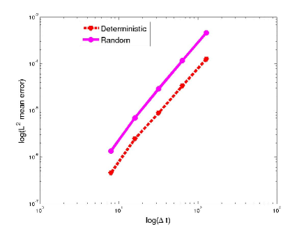
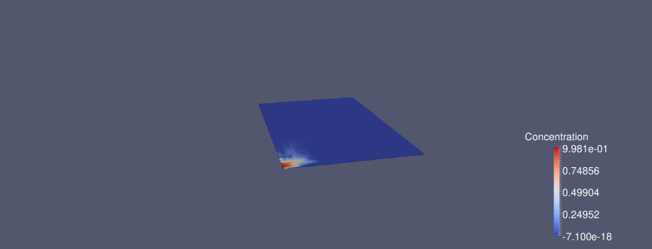
Figure 1: Graph (a) shows the convergence of the exponential Rosenbrock scheme with deterministic initial data $u_{0}=0$ and random initial data following uniform distribution in the interval $[0,1]$, at the final time $T=8192$ (large time). The convergence orders in time corresponding to the initial value $u_{0}=0$ and the random initial data are respectively $1.9978$ and $2.0914$, which are in agreement with the theoretical results in Theorem 2.2. The concentration field for the initial solution $u_{0}=0$ at final time $T=8192$ is presented in (b).

References

- [1] A. Andersson, S. Larsson, Weak convergence for a spatial approximation of the nonlinear stocahstic heat equation, Maths. Comput. 299(85) (2016), 1335–1358.
- [2] M. Caliari, A. Ostermann, Implementation of exponential Rosenbrock-type integrators, Appl. Numer. Math., 59(3-4)(2008), 568–581.
- [3] M. P. Calvo, C. Palencia, A class of explicit multistep exponential integrators for semilinear problems, Numer. Math., (102)(3) (2006), 367–381.
- [4] F. Casas, A. Murua, An efficient algorithm for computing the Baker-Campbell-Hausdorff series and some of its applications, J. Math. Phys. 50(2009), 033513.
- [5] M. A. Christie and M. J. Blunt. Tenth SPE comparative solution project: A comparison of upscaling techniques. SPE Reservoir Evaluation & Engineering, 4(4):308–317, 2001.
- [6] M. Crouzeix, V. Thomée, On the discretization in time of semilinear parabolic equations with nonsmooth initial data, Math. Comput., 49(180)(1987), 359–377.
- [7] H. Fujita, T. Suzuki, Evolutions problems (part1), in: P. G. Ciarlet and J. L. Lions(eds.), Handb. Numer. Anal., vol. II, North-Holland, 1991, pp. 789–928.
- [8] M. A. Gondal, Exponential Rosenbrock integrators for option pricing, J. Comput. Appl. Math., 234(4)(2010), 1153–1160.
- [9] C. González, A. Ostermann, C. Palencia and M. Thalhammer, Backward Euler discretization of fully nonlinear parabilic problems, Math. Comput., 71(237)(2001), 125–145.
- [10] D. Henry, Geometric theory of semilinear parabolic equations, Lect. Notes Math.,vol. 840, Springer, 1981.
- [11] M. Hochbruck, A. Ostermann, Exponential integrators, Acta Numer. (2010), 209–286.
- [12] M. Hochbruck, A. Ostermann, Explicit exponential Runge-Kutta methods for semilinear parabolic problems, SIAM J. Numer. Anal., 43(3)(2005), 1069–1090.
- [13] M. Horcbruck, A. Ostermann, and J. Schweitzer, Exponential Rosenbrock-type methods, SIAM J. Numer. Anal., 47(1)(2009), 786–803.
- [14] C. Johnson, S. Larsson, V. Thomée, L. B. Wahlbin, Error estimates for spatially discrete approximations of semilinear parabolic equations with nonsmooth initial data, Math. Comput., 49(180)(1987), 331–357.
- [15] R. Kruse, S. Larsson, Optimal regularity for semilinear stochastic partial differential equations with multiplicative noise, Electron. J. Probab. 17(65) (2012), 1-19.
- [16] R. Kruse, Optimal error estimates of Galerkin finite element methods for stochastic partial differential equations with multiplicative noise, IMA J. Num. Anal. 34 (2014), 217-251.
- [17] M. Kovács, S. Larsson, F. Lindgren, Strong convergence of the finite element method with truncated noise for semilinear parabolic stochastic equations with additive noise, Numer. Algor., 53 (2)(2010), 309–320.
- [18] S. Larsson, Nonsmooth data error estimates with applications to the study of the long-time behavior of finite element solutions of semilinear parabolic problems, Preprint 1992-36, Department of Mathematics, Chalmers University of Technology.
- [19] G. J. Lord, C. E. Powell, T. Shardlow, An introduction to computational stochastics PDES, Cambridge University press, 2014.
- [20] G. J. Lord, A. Tambue, Stochastic exponential integrators for the finite element discretization of SPDEs for multiplicative and additive noise, IMA J. Numer. Anal., 33(2)(2013), 515–543.
- [21] C. Lubich, A. Ostermann, Runge-Kutta time discretization of reaction-diffusion and Navier-Stokes equations: nonsmooth-data error estimates and applications to long-time behaviour, Appl. Numer. Math., 22(1-3)(1996), 279–292.
- [22] W. Magnus, On the exponential solution of differential equations for a linear operator, Commun. Pure Appl. Math. 7(1954), 649-673.
- [23] B. Mielnik, J. plebanski, Combinatorial approach to Baker-Campbell-Hausdorff exponents, Ann. Inst. Henri Poincaré A 12(3)(1970), 215-254.
- [24] J. D. Mukam, A. Tambue, Strong convergence analysis of the stochastic exponential Rosenbrock scheme for the finite element discretization of semilinear SPDEs driven by multiplicative and additive noise, J. Sci. Comput. 74(2)(2018), 937-978.
- [25] A. Ostermann, M. Thalhammer, Convergence of Runge-Kutta methods for nonlinear parabolic equations, Appl. Numer. Math., 42 (1-3)(2002), 367–380.
- [26] A. Ostermann, M. Thalhmmer, Non-smooth data error estimates for the linearly implicit Runge-Kutta methods, IMA J. Numer. Anal., 20(2) (2000), 167–184.
- [27] A. Ostermann, M. Thalhammer, W. Wright, A class of explicit exponential general linear methods, BIT Numer. Math. , 46(2) (2006), 409–431.
- [28] A. Pazy, Semigroups of linear operators and applications to partial differential equations, Applied Mathematical Sciences, volume 44, Springer-Verlag, New York, 1983.
- [29] D. Scholz, M. Weyrauch, A note on the Zassenhaus product formula, J. Math. Phys. 47(3)(2006), 033505.
- [30] J. Schweitzer, The exponential Rosenbrock-Euler for nonsmooth initial data, Preprint 2015, Karlsruhe Institute of Technology.
- [31] J. Schweitzer, The exponential Rosenbrock-Euler method with variable time step sizes for nonsmooth initial data, Technical report 2014, Karlsruhe Institute of Technology.
- [32] A. Tambue, An exponential integrator for finite volume discretization of a reaction-advection-diffusion equation, Comput. Math. Appl. , 71(9) (2016), 1875–1897.
- [33] A. Tambue, I. Berre, J. M. Nordbotten, Efficient simulation of geothermal processes in heterogeneous porous media based on the exponential Rosenbrock-Euler and Rosenbrock-type methods, Adv. Water Resour., 53(2013), 250–262.
- [34] A. Tambue, J. M. T. Ngnotchouye, Weak convergence for a stochastic exponential integrator and finite element discretization of stochastic partial differential equation with multiplicative & additive noise, Appl. Num. Math. 108(2016), 57-86.
- [35] V. Thomée, Galerkin finite element methods for parabolic problems, Springer Ser. Comput. Math., 2006.