Active Network Alignment: A Matching-Based Approach

Abstract.

Network alignment is the problem of matching the nodes of two graphs, maximizing the similarity of the matched nodes and the edges between them. This problem is encountered in a wide array of applications—from biological networks to social networks to ontologies—where multiple networked data sources need to be integrated. Due to the difficulty of the task, an accurate alignment can rarely be found without human assistance. Thus, it is of great practical importance to develop network alignment algorithms that can optimally leverage experts who are able to provide the correct alignment for a small number of nodes. Yet, only a handful of existing works address this active network alignment setting.

The majority of the existing active methods focus on absolute queries (“are nodes $a$ and $b$ the same or not?”), whereas we argue that it is generally easier for a human expert to answer relative queries (“which node in the set $\{b_{1},\ldots,b_{n}\}$ is the most similar to node $a$?”). This paper introduces two novel relative-query strategies, TopMatchings and GibbsMatchings, which can be applied on top of any network alignment method that constructs and solves a bipartite matching problem. Our methods identify the most informative nodes to query by sampling the matchings of the bipartite graph associated to the network-alignment instance.

We compare the proposed approaches to several commonly-used query strategies and perform experiments on both synthetic and real-world datasets. Our sampling-based strategies yield the highest overall performance, outperforming all the baseline methods by more than 15 percentage points in some cases. In terms of accuracy, TopMatchings and GibbsMatchings perform comparably. However, GibbsMatchings is significantly more scalable, but it also requires hyperparameter tuning for a temperature parameter.

1. Introduction

The network-alignment problem, also known as graph matching (Yan et al., 2016) or graph reconciliation (Korula and Lattanzi, 2014), asks to find a matching between the nodes of two graphs so that both $(i)$ node-attribute similarities and $(ii)$ structural similarities between the matched nodes are maximized. This is an ubiquitous problem with application areas ranging from biological networks (Clark and Kalita, 2014) to social networks (Goga et al., 2015; Zhang and Yu, 2015), ontologies (Shvaiko and Euzenat, 2013), and image matching in computer vision (Conte et al., 2004). For instance, in the case of social networks, one might be interested in aligning the friendship graphs of two social-networking services in order to suggest new friends for the users.

Typically, some of the network nodes are easy to align automatically if they, for example, share a unique name. Other nodes can be considerably more ambiguous and thus fully-automatic methods are likely to align them incorrectly. In the active version of the network-alignment problem, such difficult cases are redirected to human experts who act as oracles. In this way, the alignment process is judiciously enhanced by involving humans in the loop.

The idea of algorithms that select which data to be labeled in order to improve accuracy is not new; in fact, this is the main focus of active learning. Research in this area aims to identify effective ways for utilizing access to labeling oracles, such as human experts. Although there is a lot of research in active learning for classification or clustering problems, few studies have tackled the problem of active network alignment.

To the best of our knowledge, active network-alignment methods appear mostly in the domain of ontology matching (Jiménez-Ruiz et al., 2012; Sarasua et al., 2012; Shi et al., 2009). These methods ask the human experts to assess whether two given nodes are a match or not, and thus, focus on identifying the most useful pair of nodes to query. The limitation of this approach is that absolute yes/no questions can be very hard to answer for a human if no context about alternative candidate matches is provided.

In this paper, we obtain human feedback, where questions are asked in the following form: “Given node $v$ and a set of candidate matches $C$, which node in $C$ is the most likely match for $v$?”. To answer such relative questions, an expert needs to make only comparative judgments, which are less challenging for humans (Laming, 2003), despite the fact that the expert needs to consider more nodes at once. Additionally, the expert may be given an opportunity to say that none of the candidate matches is correct. In this scenario, the querying is more similar to the absolute querying scheme, but it may still be easier for the expert since more context is provided to answer the question. Although in certain scenarios the absolute querying scheme may be more appropriate, this work focuses only on comparing different relative approaches.

Given the above relative querying scheme, our framework for active network alignment is based on a novel algorithmic idea for identifying the best questions to ask to the experts. Since access to experts is typically costly, the objective is to maximize the alignment accuracy for a given number of queries.

A well-established approach in active learning is to label the data points for which the current model is least certain as to what the correct output should be (Settles, 2010). Accordingly, we introduce novel ways of quantifying the uncertainty introduced by each node in the network-alignment process. Using these measures we ask queries that resolve most of the uncertainty, and therefore, only few queries suffice to obtain an alignment of high accuracy.

In the classic (non-active) network-alignment problem the input consists of two networks: a source network $G_{s}=(V_{s},E_{s})$ and a target network $G_{t}=(V_{t},E_{t})$. Finding an alignment is often reduced into the problem of finding a matching on a weighted bipartite graph $H=(V_{s},V_{t},E_{h})$, where the weights incorporate both attribute and structural similarities. Examples of such methods include L-Graal (Malod-Dognin and Pržulj, 2015), Natalie (El-Kebir et al., 2015; Klau, 2009), NetAlignMP++ (Bayati et al., 2013), and IsoRank (Singh et al., 2008).

In this paper we propose a new approach for active network alignment, which can be employed on top of any matching-based (non-active) network-alignment method. The main idea is to sample a set of matchings $\mathcal{M}_{\ell}$, use the resulting distribution to quantify the certainty of each node, and identify which node to query based on this certainty. We study and experiment with two alternative methods for obtaining a set of sampled matchings, GibbsMatchings, where Gibbs sampling is employed to sample matchings according to their score, and TopMatchings, where the top-$\ell$ matchings are taken in the sample. We also experiment with different methods for estimating node certainty, using entropy, the expected certainty of the unlabeled nodes, as well as a consensus-based criterion.

Our experiments with real and synthetic data show that the proposed strategies perform consistently well and in some cases they outperform our baseline methods by more than 15% in accuracy. The baseline methods include three previously proposed query strategies as well as random querying. When comparing the two proposed methods, GibbsMatchings and TopMatchings, we obtain a robustness-scalability trade-off: GibbsMatchings is significantly more scalable but it is also sensitive to the choice of a temperature parameter $\beta$.

Our main contributions are summarized as follows.

• We formalize a relative-judgment framework for active network alignment.

• We develop an active-querying framework, which can be employed on top of any network-alignment method that finds an alignment using maximum-weight bipartite matching. Indeed, several state-of-the-art network-alignment methods follow this approach. We also explore two algorithms that instantiate this framework: GibbsMatchings and TopMatchings.

• We conduct experiments with real and synthetic datasets, demonstrating the superiority of our algorithms compared to several previously proposed baseline methods. We also show that our algorithms can be parallelized without significantly compromising the accuracy of the methods.

• The code and the data used in the experiments are publicly available at: https://github.com/ekQ/active-network-alignment

Roadmap: The paper is organized as follows. In Section 2 we review the related work. Our problem formulation is provided in Section 3 and our algorithm in Section 4. Section 5 presents the experimental evaluation of our method and a comparison with baselines. We conclude in Section 6.

2. Related work

Numerous methods have been developed for the non-active network-alignment problem. The problem has drawn particular attention in the bioinformatics domain (El-Kebir et al., 2015; Hashemifar and Xu, 2014; Klau, 2009; Kuchaiev et al., 2010; Liao et al., 2009; Malod-Dognin and Pržulj, 2015; Singh et al., 2008), due to the interest in the the task of matching protein-protein interaction networks; a recent survey in the area is provided by Elmsallati et al. (Elmsallati et al., 2016). Non-active network alignment methods are classified according to how the matching cost is defined and how they algorithmically proceed to finding a solution. For example, IsoRank (Singh et al., 2008) and IsoRankN (Liao et al., 2009), which are among the earliest-developed methods, utilize a PageRank-type computation to recursively compute node similarity via the similarity of the nodes’ neighbors. Natalie (El-Kebir et al., 2015; Klau, 2009) formulates the alignment task as a quadratic assignment problem, which it then solves using Lagrangian relaxation combined with a subgradient optimization; more details are given in Section 4.2. The Graal (Kuchaiev et al., 2010; Kuchaiev and Pržulj, 2011; Malod-Dognin and Pržulj, 2015) family of alignment methods enhance the matching scoring function with topological similarity features, such as graphlet degree signatures (Pržulj, 2007). L-Graal (Malod-Dognin and Pržulj, 2015) is a recent algorithm in the Graal family, which incorporates the Lagrangian-relaxation framework of Natalie, and is shown to outperform several other state-of-the-art methods.

In addition to bioinformatics, the non-active network-alignment problem has been studied in different application areas, such as ontology matching (Aumueller et al., 2005; Doan et al., 2004) and social-network matching (Korula and Lattanzi, 2014).

As discussed earlier, our active network-alignment framework can be employed on top of any non-active method that maps the alignment problem into a weighted bipartite graph-matching problem. Many of the methods discussed above fall in this category, e.g., L-Graal (Malod-Dognin and Pržulj, 2015), Natalie (El-Kebir et al., 2015; Klau, 2009), NetAlignMP++ (Bayati et al., 2013), and IsoRank (Singh et al., 2008). In our experimental evaluation we use Natalie and NetAlignMP++, which are state-of-the-art methods that have been shown to have a robust performance in several independent studies (Bayati et al., 2013; Clark and Kalita, 2014; El-Kebir et al., 2015; Malod-Dognin and Pržulj, 2015).

The problem of active network alignment has been previously studied by Cortés and Serratosa (Cortés and Serratosa, 2013). Compared to our work, they focus on a more limited class of network-alignment methods that return a probability matrix for different matches, making the quantification of uncertainty more straightforward. However, some of their query strategies are also applicable to our setting and thus, in our experiments, we adopt two baseline strategies from their work, namely lccl and Margin. Another closely-related line of work is active ontology matching. Shvaiko and Euzenat (Shvaiko and Euzenat, 2013) list it as one of the important areas for future work in their recent survey on ontology matching. Existing work on active ontology matching focuses on absolute queries (Jiménez-Ruiz et al., 2012; Sarasua et al., 2012; Shi et al., 2009), and thus, not directly comparable with our approach.

Active-learning approaches have been developed also for other related problems. Charlin et al. (Charlin et al., 2012) develop an active-learning method for many-to-many matching problems encountered in recommender systems, comparing different absolute-querying strategies. Another area where active learning has been studied and where data is in a network format is the inference problem for Gaussian fields (Macskassy, 2009; Zhu et al., 2003). Macskassy (Macskassy, 2009) finds an empirical risk minimization (erm) to be the best method to find the next instance to query but due to the high computational complexity of erm, he proposes to use the betweenness centrality as a filter to select a subset of nodes for which erm is applied to. Finally, Bilgic et al. (Bilgic et al., 2010) introduce an active learning method for collectively classifying networked data.

3. Problem formulation

Before defining the active network alignment problem, we first discuss the non-active version of the problem.

Network alignment: In the standard network-alignment problem we consider two input graphs $G_{s}=(V_{s},E_{s})$ and $G_{t}=(V_{t},E_{t})$, the source and the target graph. The adjacency matrices of the two graphs are denoted by $A_{s}$ and $A_{t}$, respectively. Throughout we assume that the smaller graph is aligned to the larger one, that is, $|V_{s}|\leq|V_{t}|$. In addition, we consider that a similarity function $\sigma:V_{s}\times V_{t}\rightarrow\mathbb{R}$ is available, which measures the similarity between pairs of nodes $i\in V_{s}$ and $j\in V_{t}$. The similarity function $\sigma$ depends on the application at hand.

The objective of the network-alignment problem is to find a matching between the nodes of the two networks. More specifically, we want to align the nodes of the source graph $V_{s}$ to the nodes of the target graph $V_{t}$. Formally, we want to find $M=\{(i,j)\}\subseteq V_{s}\times V_{t}$ so that each node of $V_{s}$ and $V_{t}$ appears at most one time in $M$. A high-quality alignment should satisfy the following properties: ($i$) nodes in $V_{s}$ should match to similar nodes in $V_{t}$, according to $\sigma$, and ($ii$) the endpoints of each edge in $E_{s}$ should match to nodes in $V_{t}$ that are connected by edges in $E_{t}$.

For each node $v\in V_{s}$ we consider a set of candidate matching nodes $\mathcal{C}_{v}\subseteq V_{t}$. Those are the only nodes in $V_{t}$ that $v$ can be matched to. In this paper we assume that the sets $\mathcal{C}_{v}$ are given. In practice, the sets $\mathcal{C}_{v}$ are computed by a simple heuristic, e.g., considering all nodes in $V_{t}$ whose feature-based similarity to $v\in V_{s}$ exceeds a certain threshold. When the candidate sets are small compared to $V_{t}$, the problem is sometimes called sparse network alignment.

Global network-alignment methods formulate an objective function that captures the above properties, and then devise algorithms for optimizing this objective.

In some applications, it is desirable to leave nodes unmatched if no suitable match is found. This can be achieved without having to change the problem formulation by adding a special “gap” node to the target graph for each node in the source graph. The gap nodes are isolated and the user has to define a similarity value (which can also be negative) between the source nodes and the gap nodes, which controls the cost of leaving a source node unmatched.

Figure 1. An illustration of the network-alignment problem. The task is to align two input networks $G_{s}$ and $G_{t}$. Some nodes and/or edges from either network may be left unmatched. Letters and colors are used to indicate the sets of candidate matching nodes, e.g., $\mathcal{C}_{A}=\{A_{1},A_{2},A_{3}\}$, $\mathcal{C}_{B}=\{B_{1},B_{2}\}$, and $\mathcal{C}_{C}=\{C_{1},C_{2}\}$.

An example of the network-alignment problem is shown in Figure 1. We use letters and colors to indicate sets of matching nodes. Indicatively, in an application of aligning social networks, one can think of $A=\;$Andres, $A_{1}=\;$Andre, $A_{2}=\;$Andrew, $A_{3}=\;$Andreas, while $B=\;$Brendon, $B_{1}=\;$Brenden, $B_{2}=\;$Brendan, etc.

Active network alignment: Assume now that we have access to an oracle, for example, a human expert, with whom we can interact in the form of queries and obtain partial information about the correct alignment of the two networks $G_{s}$ and $G_{t}$.

As already discussed, we focus on interaction with the oracle that takes the form of the following queries:

Given a node $v$ in the source network $G_{s}$, and a set of candidate matches $\mathcal{C}_{v}$ in the target network $G_{t}$, which node from $\mathcal{C}_{v}$ should be matched to $v$?

The oracle returns an answer $u\in\mathcal{C}_{v}$ and the algorithm proceeds to aligning $G_{s}$ with $G_{t}$ given that $v\in V_{s}$ is matched with $u\in V_{t}$. Depending on the application, one of the candidate matches $\mathcal{C}_{v}$ may be the gap node of $v$.

The problem of active network alignment is to select the most informative node $v\in V_{s}$ for which to ask the oracle to reveal the correct matched node $u\in V_{t}$. More specifically, we aim to solve the following problem.

Problem 1 (ActiveNetworkAlignment).

Given a source network $G_{s}=(V_{s},E_{s})$ and a target network $G_{t}=(V_{t},E_{t})$, select the node $v\in V_{s}$ for which to ask an oracle to reveal the correct matched node $u\in V_{t}$ so that the alignment accuracy for the remaining nodes in $V_{s}$ is maximized.

The alignment accuracy in Problem 1 is computed by fixing the alignment of $v$ to $u$, then aligning the remaining nodes using a standard (non-active) network alignment method, and finally by computing the fraction of correctly aligned unqueried nodes in $V_{s}$.

A natural way to approach Problem 1 is to design a function $\mathrm{Cert}\left(v\mid G_{s},G_{t}\right)$ that quantifies the certainty associated with each $v\in V_{s}$ with respect to its match in $V_{t}$. Nodes with low certainty scores are good candidates for being the query node, since these nodes would otherwise be more likely to decrease the alignment accuracy. The active-learning framework provides general principles for designing such a function. We deploy these ideas in order to design and experiment our $\mathrm{Cert}$ function. More details on this are given in Sections 4 and 5.

In the example of Figure 1, we see that $A$ in $G_{s}$ is most similar to $A_{1}$, $A_{2}$, and $A_{3}$ in $G_{t}$. If $A$ is matched to $A_{1}$ or $A_{2}$, then $B$ should be uniquely matched to $B_{1}$. If $A$ is matched to $A_{3}$, then $B$ should be uniquely matched to $B_{2}$ and $C$ to $C_{2}$. Thus, matching node $A$ first, to a large extent, determines the rest of the alignment. On the other hand, matching $B$ or $C$ first does not determine the rest of the alignment with the same level of certainty. We conclude that, in this example, it is a good strategy to ask the oracle to provide us with the correct alignment for node $A$.

4. Matching-based active network alignment

In this section, we present the proposed strategy for active network alignment. Our strategy identifies which node $v\in V_{s}$ to query via a novel approach for quantifying the certainty of each node. The main idea is as follows: instead of solving the alignment problem to find only a single matching (the optimal network alignment), we sample a number of high-quality matchings (near-optimal network alignments), and then, compute the certainty of each node by considering the distribution of its matched nodes on the sampled matchings.

We study two different methods for sampling matchings; GibbsMatchings, where matchings are sampled according to their score (so better matchings have higher probability of being included in the sample), and TopMatchings, where the top-$\ell$ matchings are considered. We also consider different alternatives for computing node certainty based on the sampled matchings.

We now discuss our approach in more detail. We start by describing our strategy at a high level, and then proceed to the description of each of its components and different alternatives.

4.1. Overview

The general active network alignment approach, in which nodes are queried iteratively, can be summarized as follows: In every iteration pick a node $\hat{v}\in V_{s}$. The node $\hat{v}$ together with its set of candidate matching nodes $\mathcal{C}_{\hat{v}}\subseteq V_{t}$ is shown to the (human) oracle, and the oracle selects a node $\hat{u}\in\mathcal{C}_{\hat{v}}$ as the best match for $\hat{v}$. Assert that $\hat{u}$ is the best matching for $\hat{v}$ by updating the candidate node sets so that $\mathcal{C}_{\hat{v}}=\{\hat{u}\}$, and removing $\hat{u}$ from all other sets of candidate nodes. When the budget of oracle queries is exhausted, solve the remaining network alignment problem to align the unqueried nodes. Pseudocode for this approach is shown in Algorithm 1 (different steps of the algorithm are explained later in this section).

1:Input: $G_{s}=(V_{s},E_{s})$, $G_{t}=(V_{t},E_{t})$, candidate matches $\mathcal{C}$, and query budget $k$.

2:Output: An alignment between $V_{s}$ and $V_{t}$.

3:for $i=1,\ldots,k$ do

4:     $H=$ NetworkAlignment$\left(G_{s},G_{t}\mid\mathcal{C}\right)$

5:     $\hat{v}=\mathrm{argmin}_{v\in V_{s}}\mathrm{Cert}\left(v\mid H,G_{s},G_{t}\right)$

6:     $\hat{u}=\text{\sc Oracle\-Query}(\hat{v},\mathcal{C}_{\hat{v}})$, with $\hat{u}\in\mathcal{C}_{\hat{v}}$

7:     $\mathcal{C}_{\hat{v}}=\{\hat{u}\}$ $\triangleright$ Update candidate matches.

8:     for $v\in V_{s}\setminus\{\hat{v}\}$ do

9:         $\mathcal{C}_{v}=\mathcal{C}_{v}\setminus\{\hat{u}\}$      

10:$H=$ NetworkAlignment$\left(G_{s},G_{t}\mid\mathcal{C}\right)$

11:return BipartiteMatching($H$)

Algorithm 1 The general active network alignment framework.

Our main contribution, is the methodology for quantifying the certainty of the candidate nodes to be queried at every iteration of Algorithm 1. Our approach consists of the following steps.

• Construct a weighted bipartite graph $H=(V_{s},V_{t},E_{h})$ that forms the basis for the matching-based network-alignment algorithm.

• Sample a set $\mathcal{M}_{\ell}$ of $\ell$ high-quality matchings in $H$.

• For each node $v\in V_{s}$, estimate the certainty we have about the correct match for $v$. These certainty values, $\mathrm{Cert}(v)$, are computed using the information in the set of sampled matchings $\mathcal{M}_{\ell}$.

• Identify the node $\hat{v}\in V_{s}$ with the least certainty, and query the oracle for selecting the best match of $\hat{v}$ among the set of candidate matching nodes $\mathcal{C}_{\hat{v}}\subseteq V_{t}$.

For sampling a set of matchings $\mathcal{M}_{\ell}$ we consider two alternatives: GibbsMatchings (sample matchings according to their score) and TopMatchings (take the top-$\ell$ matchings); those are discussed in Section 4.3. We also consider three different ways of estimating node certainty (Step 3) presented in Section 4.4. First we discuss how to construct the weighted bipartite graph $H=(V_{s},V_{t},E_{h})$ on which the set of sampled matchings $\mathcal{M}_{\ell}$ is obtained.

4.2. Constructing the bipartite graph $\boldsymbol{H}$

Our strategy is applicable to any NetworkAlignment algorithm that is based on solving a bipartite-matching problem. In our experiments, we use Natalie (El-Kebir et al., 2015) and NetAlignMP++ (Bayati et al., 2013), two state-of-the-art algorithms. Both methods aim to solve the following quadratic integer program, adopting, however, different approaches.

Integer-programming formulation: The IP formulation of Natalie and NetAlignMP++ introduces a variable $x_{ij}$ for each pair of nodes $i\in V_{s}$ and $j\in V_{t}$. The variable $x_{ij}$ is set to 1 if $i$ is matched to $j$, while it is set to 0 otherwise. We also use $\Delta(v)$, for $v\in V_{s}\cup V_{t}$, to denote the set of all pairs $\{(i,j)\}$ for which $v=i$ or $v=j$, and $A_{s;ik}$ ($A_{t;ik}$) to denote whether there is an edge between nodes $i$ and $k$ in the source (target) graph.

$$\max_{x}\quad \sum_{(i,j)\in V_{s}\times V_{t}}\sigma(i,j)x_{ij}$$

$$+g\sum_{(i,j)\in V_{s}\times V_{t}}\sum_{(k,\ell)\in V_{s}\times V_{t}}A_{s;ik}A_{t;j\ell}x_{ij}x_{k\ell},$$

such that $$\sum_{(i,j)\in\Delta(v)}x_{ij}\leq 1,\quad\textmd{for all }v\in V_{s}\cup V_{t},$$

$$x_{ij}\in\{0,1\},\quad\textmd{for all }(i,j)\in V_{s}\times V_{t}.$$

In the above integer program, each pair of matched nodes $i$ and $j$ contributes a reward of value $\sigma(i,j)$, while an additional reward of value $g$ is given if an edge in $E_{s}$ is matched to an edge in $E_{t}$. The user-defined parameter $g$ quantifies the relative importance between correctly-matched nodes and correctly-matched edges, and it is typically set based on prior knowledge or cross-validation. The inequality constraint ensures that the solution is a matching.

Solution via Lagrangian relaxation: Natalie, originally proposed by Klau (Klau, 2009), solves the quadratic integer program by first linearizing it and then employing a Lagrangian relaxation technique. Klau shows that the original integer program is NP-hard, but remarkably, by relaxing a symmetry constraint for the linearized quadratic terms, the problem becomes solvable in polynomial time via multiple maximum-weight bipartite matchings.

Natalie iteratively updates the Lagrangian multipliers $\lambda$ for the relaxed constraints using subgradient optimization. The solutions of the relaxed problem provide upper bounds for the original problem, whereas the feasible solutions, which can be directly extracted from the relaxed solutions, provide lower bounds.

The best feasible solution found provides the bipartite graph $H$ for our active strategy.

Solution via message passing: The NetAlignMP++ algorithm, proposed by Bayati et al. (Bayati et al., 2013), solves the same optimization problem using a belief propagation (BP) approach. This approach makes local, greedy updates by passing messages between the neighboring nodes. To obtain an integral solution, NetAlignMP++ constructs and solves a maximum-weight matching problem based on the BP messages at every iteration of the algorithm.

Again, we set $H$ to correspond to the matching problem that gives the best solution.

Due to space constraints, we do not discuss in detail how the weights of the edges of the bipartite graphs are set. Note, however, that the weights aim at capturing both the feature-based and structural similarities of the matching nodes, and the higher the weight the more similar the nodes are. For more details we refer the reader to the original papers (Bayati et al., 2013; El-Kebir et al., 2015).

4.3. Sampling matchings

Next we present two approaches for sampling matchings: GibbsMatchings, which first defines a probability distribution over the space of matchings and then employs Gibbs sampling to draw samples from this space, and TopMatchings, which computes the top-$\ell$ matchings.

Gibbs sampling for matchings: Markov chain Monte Carlo techniques are popular for drawing samples from complex multi-dimensional distributions (Bishop, 2009). In order to apply these methods to sample matchings $M$, we need to define a probability distribution over the space of matchings induced by the bipartite graph $H$. Similar to Volkovs and Zemel (Volkovs and Zemel, 2012), we use the standard Gibbs form

$$P\left(M\mid H\right) =\frac{1}{Z(M,\beta)}\exp\left(-\frac{1}{\beta}E(M,H)\right)$$

(1) $$=\frac{1}{Z(M,\beta)}\exp\left(\frac{1}{\beta}\sum_{v\in V_{s}}H_{v,M(v)}\right),$$

where $M(v)$ denotes the node to which $v$ is matched to in $M$, $Z(M,\beta)$ is the partition function that normalizes the distribution, and $\beta$ is a “temperature” constant that defines the smoothness of the distribution. The value of $\beta$ is optimized using a training dataset, as discussed in Section 5.3.

We sample $\ell$ matchings $\mathcal{M}_{\ell}=\{M_{1},\ldots,M_{\ell}\}$ from this distribution as follows: we initialize $M$ with the maximum-weight matching. Then at each iteration $i$, we go through the nodes in $V_{s}$ in a random order and for each node $v\in V_{s}$, we pick one of the candidate matching nodes $u\in\mathcal{C}_{v}$ uniformly at random. Next we consider re-assigning $v$ to $u$ and $v^{\prime}$ to $M(v)$ where $v^{\prime}$ is the node currently matched to $u$ if any. If $M(v)$ is not among the candidate matches of $v^{\prime}$, we pick another node $u$ uniformly at random among the remaining candidates of $v$ until a possible re-assignment has been found ($v$ can always be re-assigned to its current match $M(v)$). The new matching $M^{\prime}$, which would result from the re-assignment, is realized and the update $M\leftarrow M^{\prime}$ performed with probability

$$P\left(M^{\prime}\mid M,H\right)=\frac{\exp\left(-\frac{1}{\beta}E(M^{\prime},H)\right)}{\exp\left(-\frac{1}{\beta}E(M,H)\right)+\exp\left(-\frac{1}{\beta}E(M^{\prime},H)\right)}$$

(2) $$=\frac{\exp\left(\frac{1}{\beta}\left(H_{v,u}+H_{v^{\prime},M(v)}\right)\right)}{\exp\left(\frac{1}{\beta}\left(H_{v,M(v)}+H_{v^{\prime},u}\right)\right)+\exp\left(\frac{1}{\beta}\left(H_{v,u}+H_{v^{\prime},M(v)}\right)\right)}.$$

Once each node has been processed, we let $i$-th sample be $M_{i}\leftarrow M$. Then, we generate a new random permutation of the nodes $V_{s}$ and repeat the process until $\ell$ samples have been drawn. We call this method GibbsMatchings. Assuming that each node has $c$ candidate matches, the worst-case complexity of GibbsMatchings is $\mathcal{O}(\ell c|V_{s}|)$.

Volkovs and Zemel (Volkovs and Zemel, 2012) note that Gibbs sampling is often found to mix slowly and get trapped in local modes. In our case, such slow mixing implies that we will end up exploring only the areas around the maximum weight matching, which is the starting point of the sampling. However, even if this happens, we do not expect it to be a problem as we indeed are interested in sampling high-quality matchings close to the optimal solution.

Top-$\ell$ maximum-weight matchings: To compute the top-$\ell$ maximum-weight matchings $\mathcal{M}_{\ell}$, we use an algorithm invented by Murty (Murty, 1968) in 1968. This algorithm first computes the best maximum-weight matching in $H$, then splits the problem into $\mathcal{O}(n)$ smaller matching problems and reconstructs the second best matching based on the solutions of the smaller problems. The process is repeated until $\ell$ matchings have been discovered, and in total, the algorithm has a running time of $\mathcal{O}(\ell n^{4})$, where $n$ is the total number of nodes in the graph, i.e., in our case $n=\max\{|V_{s}|,|V_{t}|\}$. Using a modification by Miller et al. (Miller et al., 1997), the algorithm runs in time $\mathcal{O}(\ell n^{3})$.

Figure 2. The instance of the network-alignment problem in Figure 1 is transformed to an instance of a maximum-weight matching problem. Computing the set $\mathcal{M}_{\ell}$ of $\ell=5$ matchings helps to quantify the uncertainty of a node in network alignment.

4.4. Quantifying certainty and identifying the node to query

Using uncertainty to determine which data points should be labeled is a standard active-learning strategy (Settles, 2010). The idea is to select for labeling the data points for which we are the least certain as to what the correct output should be.

A natural approach for quantifying the uncertainty of a match $M(v)$ of node $v\in V_{s}$ is to consider the marginal distribution $P\left(M(v)=u\mid H\right)$, where $u\in V_{t}$. Given the set of sampled matchings $\mathcal{M}_{\ell}$, the marginal distribution can be obtained simply by computing the fraction of samples for which node $v$ is matched to $u$. We then define the certainty of node $v$ as

(3) $$\mathrm{Cert}(v)=\max_{u\in C_{v}}P\left(M(v)=u\mid H\right).$$

The intuition for Equation (3) is that when a node $v$ is matched to the same node $u$ in most of the matchings in $\mathcal{M}_{\ell}$, then there is little uncertainty; based on the evidence in the set of sampled matchings $\mathcal{M}_{\ell}$, $u$ is a good match for $v$ and no extra information will be gained by querying $v$. On the other hand, if the evidence in $\mathcal{M}_{\ell}$ is inconclusive with respect to the best match for $v$, then $v$ should be queried. Accordingly, the proposed strategy is to query the node $\hat{v}$ with the least certainty, i.e.,

(4) $$\hat{v}=\mathrm{argmin}_{v\in V_{s}}\mathrm{Cert}(v).$$

To obtain further intuition for the proposed method, consider again the example in Figure 1. The bipartite graph $H$ for this example is shown on the left in Figure 2.

Now assume that we draw a sample of $\ell$ matchings in this bipartite graph. A sample of five matchings is shown in Figure 2. For each node $v\in V_{s}$ we can compute the distribution of the nodes in $V_{t}$ that $v$ is matched to in these five matchings. A node with high uncertainty is a node that is matched to many different nodes in $V_{t}$ and the distribution of matches is well-balanced. In the example of Figure 2, the distribution of matchings for nodes $A$, $B$, and $C$ is $\{A_{1}:40\%,\,A_{2}:40\%,\,A_{3}:20\%\}$, $\{B_{1}:80\%,\,B_{2}:20\%\}$, and $\{C_{1}:40\%,\,C_{2}:60\%\}$, respectively. From these distributions one can argue that node $A$ has the highest uncertainty.

An alternative measure for the certainty of a node would be to study entropy, which is commonly used in active learning (Settles and Craven, 2008; Roy and McCallum, 2001). However, in our experiments we found that Equation (3) consistently outperformed a method which defined certainty as the negative entropy of the marginal distribution. Thus we do not report experimental results using the entropy-based method.

A limitation of Equation (3) is that it measures certainty only locally and thus it does not capture the effect that knowing the matching for a given node $v$ would have on the remaining alignment. Therefore, we consider also another alternative query strategy which queries the node $\hat{v}$ such that once $\hat{v}$ is queried and its match is known, the expected certainty of the remaining nodes is maximized. That is,

(5) $$\hat{v}=\arg\max_{v\in V_{s}}\sum_{u\in C_{v}}\left(P\left(M(v)=u\mid H\right)\sum_{v^{\prime}\in V_{s}\setminus v}\mathrm{Cert}(v^{\prime})\right).$$

This approach is inspired by previous works in sensor placement (Krause et al., 2008; Krause and Guestrin, 2007) and active learning (Macskassy, 2009). As pointed out by the previous works, a limitation of this approach is its high computational complexity, which in our case is given by $\mathcal{O}(c^{2}|V_{s}|^{2})$, assuming that each node has $c$ candidate matches. In our initial experiments, it performed similarly to the simpler query strategy given in Equation (4), which is why we only consider the latter hereafter.

4.5. Batch querying

Instead of finding the best query to ask at every iteration of Algorithm 1 we can adopt a “batch” approach, where in each iteration we identify a batch of queries to ask — the ones that correspond to the nodes with the smallest $\mathrm{Cert}$ values. When considering batches of size $k^{\prime}<k$, where $k$ is the total number of queries to be made, we can achieve a speedup of the order $\lceil\frac{k}{k^{\prime}}\rceil$.

We can readily employ all the query strategies studied in this paper to query in batches. However, these strategies might yield nodes that strongly depend on each other (that is, if we knew the alignment for one node, we could easily align another node). Thus, developing more sophisticated methods for batch querying remains an interesting avenue for future research.

5. Experimental evaluation

We evaluate a number of different network-alignment query strategies on networks where the correct alignment is known. Our methodology is as follows: First, we solve the network-alignment problem with a non-active alignment method and report the alignment accuracy, that is, the fraction of correctly aligned nodes. Then we start simulating the oracle queries by fixing the nodes to their correct matches. After each query we solve the network-alignment problem given the current correct matches and report the alignment accuracy on the unqueried nodes. This process is repeated for each query strategy separately with the same initial graphs. A good strategy should use as few queries as possible to reach the desired alignment accuracy.

As mentioned earlier, the query strategies discussed in this paper can be applied on top of any (non-active) network-alignment method that results in solving a bipartite-matching problem. In the experiments, we employ the query strategies on top of two state-of-the-art alignment methods, Natalie (El-Kebir et al., 2015; Klau, 2009) and NetAlignMP++ (Bayati et al., 2013) (see Section 4.2 for a brief discussion). The query strategies as well as the non-active network alignment methods used in the experiments support leaving nodes unmatched, but in our experiments, there is always a match for each node of the source graph.

Next we describe our datasets and present an empirical comparison between GibbsMatchings, TopMatchings, and four baseline query strategies.

5.1. Datasets

We use three types of datasets. In all datasets, there is a sufficient degree of ambiguity in the node attributes so that for each node in one graph there are several candidate matches in the other graph. Furthermore, the edges of the graphs may have been corrupted.

Preferential-attachment graphs: We generate a network using the preferential-attachment model (Barabási and Albert, 1999), which captures some of the key characteristics of social networks and has been previously used to study network-alignment methods (Korula and Lattanzi, 2014). The network consists of $1\,000$ nodes and 2 edges per new node. For each node, we sample a label from a set of 33 unique labels and treat the labels as attributes so that the similarity between two nodes is set to 1 if their labels are the same and 0 otherwise. Only the nodes with the same label are considered candidate matches, resulting in 30 candidate matches per node on average.

We make two copies of the network and in each copy we independently corrupt the edges to further complicate the alignment task. We first discard $60\,$% of the graph edges chosen at random and then add $50\,$% more edges again selected at random.

Social networks: We use the the multiplex dataset from Aarhus University (Magnani et al., 2013), which contains five networks between the employees of the Department of Computer Science. We select two of these layers, the Facebook and the lunch networks, and try to align the former to the latter. Since the dataset only contains anonymized user identifiers, we again sample a label for each node so that on average there are three people with the same label. The lunch network contains 60 people, whereas the Facebook network covers only a subset of 32 of them. While this dataset is small, it makes an interesting case study since it contains two very different types of real-world networks and the correct alignment is known.

Family trees: Aligning family trees is an import problem encountered in various online genealogy services where different people provide family tree fragments, which then, ideally, get merged into a single large family tree. We have obtained a family tree containing $64\,208$ people constructed by an individual genealogical researcher. We sample a subgraph of this network by randomly picking a seed person and doing a random walk until $1\,000$ distinct people have been discovered.

For each person we only consider the first name, last name, and birth year. Birth year is corrupted by rounding it to the nearest ten. Some of the first and last names are randomly replaced by their alternative spellings based on a list of common name variations. For example, the name Felix Ahlrooth might get replaced by Feeliks Alroot. Such name variations are frequently encountered in historical documents used in genealogical research. From both graphs independently, we discard $50$% of the edges at random.

The task is to align the subgraph into the larger graph. When selecting candidate entities for each individual in the subgraph, we find people from the larger graph born in the same decade and select four of them with the most similar names in addition to the groundtruth match. Name similarity is computed as the average Jaro-Winkler similarity (Winkler, 1990) between the first names and between the last names.

5.2. Baseline query strategies

We compare the performance of the sampling-based query strategies to four baseline strategies.

Margin: Querying data samples with a small score difference (margin) between the two most probable labels is a common approach in active learning (Settles, 2010). In the context of active network alignment, this method has been previously used by Cortés and Serratosa (Cortés and Serratosa, 2013).

Thus, given the bipartite graph $H$, Margin computes $\mathrm{Cert}(v)$ for every $v\in V_{s}$ by first finding the two edges incident to $v$ with the largest weights $w_{1}(v)$ and $w_{2}(v)$ in $H$. Then the node is scored according to

$$\mathrm{Cert}(v)=w_{1}(v)-w_{2}(v).$$

Intuitively, the larger the difference between $w_{1}(v)$ and $w_{2}(v)$, the less uncertainty there is with respect to the best match for node $v$.

lccl: The Least Confident given the Current Labelling query strategy ranks nodes according to

$$\mathrm{Cert}(v)=H_{v,M(v)},$$

where $M$ is the current matching (the maximum-weight matching in $H$) and $H_{v,M(v)}$ is the weight between node $v$ and its current match. This method was reported to yield the highest precision of the four uncertainty sampling based methods studied by Cortés and Serratosa (Cortés and Serratosa, 2013).

Betweenness: This method queries a previously unqueried node with the highest betweenness centrality in $G_{s}$. The method has been previously used by Macskassy (Macskassy, 2009).

Random: This method queries nodes from $V_{s}$ in a random order.

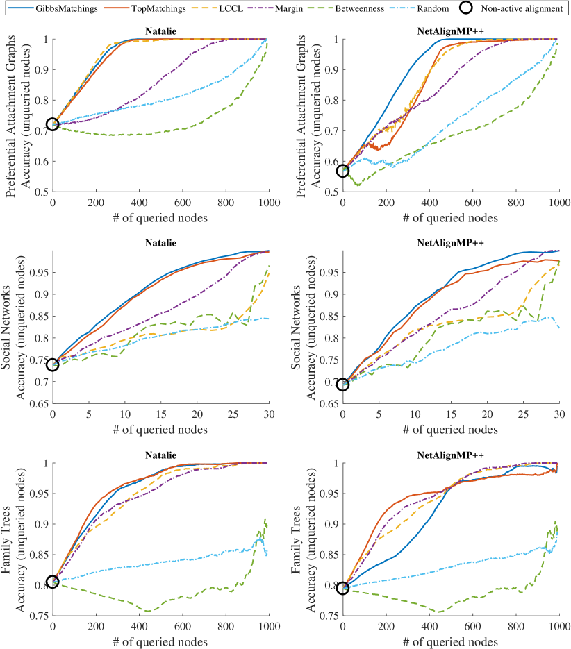
Figure 3. Alignment accuracy of the unqueried nodes for three datasets: preferential attachment graphs (top), social networks (middle), and family trees (bottom). In most cases, the proposed methods (GibbsMatchings and TopMatchings) achieve a high accuracy with fewer queries than the four baseline methods. Furthermore, the proposed active-querying strategies clearly improve the initial solution obtained by a non-active alignment method.

5.3. Query strategy comparison

Here we perform an empirical comparison of the different query strategies. For each dataset, we run a minimum of 30 random initializations of the input graphs and average the results; for the preferential-attachment graphs, we generate a new pair of input graphs at each initialization, for social networks, we sample new node labelings and for family trees a new subgraph at each initialization.

Adjusting hyperparameters: The number of matchings $\ell$ in TopMatchings is set to 30. We also tried larger values up to 3000 but this did not seem to have a significant effect on the results. In GibbsMatchings, we set the number of samples $\ell$ to 3000. Additionally, we have to choose the value of the temperature parameter $\beta$. If the value is set too high, the distribution becomes close to a uniform distribution, whereas if it is set too low, the distribution becomes very concentrated and the swaps to a lower energy state will always fail. Therefore, we first normalize the bipartite graph $H$ by dividing its values with the difference of the average minimum and maximum value of the different rows of $H$. Then we optimize $\beta$ using a separate training dataset. This dataset is generated using the preferential-attachment model, as described in Section 5.1 but with only 50 nodes per graph and 5 unique labels. Among the values we tried, $\{0.001,0.01,0.1,1\}$, we found $\beta=0.1$ to produce the most accurate predictions for the training data, and thus we fix this value for the rest of the experiments.

Results: The alignment accuracies are shown in Figure 3. On the $x$-axis, we have the number of queried nodes and on the $y$-axis, the alignment accuracy for the unqueried nodes, that is, the fraction of correctly aligned unqueried nodes.

In the top row of Figure 3, we see that by querying the 400 best nodes according to GibbsMatchings, TopMatchings, or lccl, the remaining 600 nodes get correctly aligned when using Natalie, whereas the other query strategies require at least 800 queries for obtaining a perfect alignment. For social networks (Figure 3; middle) Margin clearly outperforms lccl, while GibbsMatchings and TopMatchings outperform both of them except for when querying 26 nodes or more and using TopMatchings with NetAlignMP++. Finally, in family trees (Figure 3; bottom), GibbsMatchings and TopMatchings consistently outperform the other methods when using Natalie. With NetAlignMP++, lccl and Margin outperform the sampling methods after querying half of the nodes, and in contrast to the other experiments, GibbsMatchings performs clearly worse than TopMatchings within the first half of the queries. To understand this difference better, we ran GibbsMatchings with different temperatures and noticed that with $\beta=0.001$, GibbsMatchings obtains a comparable performance with TopMatchings. This suggests that the optimal $\beta$ value is sometimes problem dependent.

A surprising observation is that in most cases Betweenness is outperformed even by random querying. This is probably explained by the fact that Betweenness queries central nodes that have many neighbors and are thus less uncertain since the neighbors help inferring their correct alignment.

We conclude that the best overall performance is obtained using the GibbsMatchings and TopMatchings methods; lccl and Margin are both competitive baselines but in some cases they yield more than 15 percentage point lower accuracies, whereas the sampling methods perform consistently well.

5.4. Batch querying and scalability

When aligning large networks with the help of human experts, getting the responses from the humans easily becomes the bottleneck of the algorithm. To circumvent this problem, we can query batches of nodes as discussed in Section 4.5. To study the effect of batch querying on GibbsMatchings, we run an experiment on the preferential-attachment graphs and vary the batch size. Figure 4 shows the effect of the batch size on the alignment accuracy. With a batch size of 10, the accuracy is hardly affected, and even when batch size is increased to 100 nodes, the accuracy decreases by no more than $3.5$%. This shows that we can obtain accurate network alignments even when querying the experts in parallel.

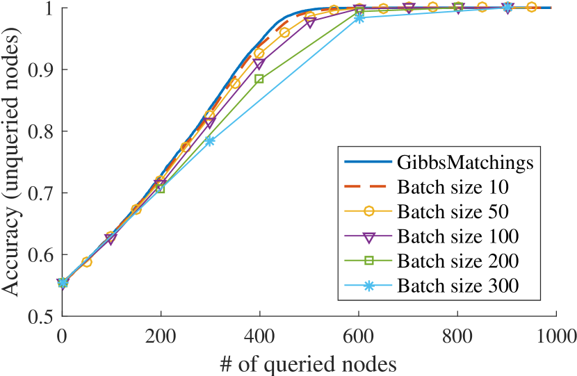
Figure 4. The effect of querying nodes in batches to the overall alignment accuracy.

Another potential bottleneck is computing the nodes to query. Table 1 lists the running times for computing a query node using TopMatchings and GibbsMatchings combined with Natalie, when aligning two preferential-attachment graphs with a varying number of nodes. The number of matchings is set to $\ell=30$ with both methods (note that in the main experiments, we used 3 000 samples with GibbsMatchings). With networks of up to 1 000 nodes, TopMatchings is not yet a significant bottleneck but when the number of nodes becomes 10 000, TopMatchings takes already 2.6 hours. GibbsMatchings, on the other hand, scales well so that and even for graphs with 100 000 nodes it only takes 10 minutes to sample 30 matchings. Furthermore, GibbsMatchings can be parallelized in a straightforward manner by running multiple independent Markov chains simultaneously.

Table 1. Running times for the proposed query methods and for the network alignment method Natalie.

Number of nodes	TopMatchings query time	GibbsMatchings query time	Alignment time
100	1.2 sec	0.03 sec	3.9 sec
1 000	21.7 sec	0.13 sec	11.0 sec
10 000	9240.5 sec	5.10 sec	48.1 sec
100 000	–	621.90 sec	372.9 sec

Finally, we also discovered that Natalie can be optimized when employing it multiple times for a sequence of similar problems. More specifically, after we have queried a node and fixed its alignment, otherwise keeping the problem unaltered, we can leverage the solution of the previous problem for solving the current problem. This is achieved by initializing the Lagrangian multipliers corresponding to the relaxed constraints by the optimal values of the multipliers in the previous run of Natalie. In our initial experiments, this strategy provided speed ups of more than $60$% for the convergence of the subgradient optimization. However, since Natalie is typically not the bottleneck of the proposed active network alignment approach, we have omitted these results.

6. Conclusions

In this paper we formalized an active-learning framework, which allows us to incorporate human feedback into the network alignment problem (also known as graph matching). In this framework, we obtain human feedback by asking relative queries to make interaction with experts easier, whereas most of the existing works on active network alignment rely on absolute queries. Moreover, we develop a scheme for selecting which nodes to obtain human feedback for. Our approach relies on sampling a set of matchings in a transformed bipartite graph, and quantifying the certainty of each node using the marginal distribution of the node. We study two alternative methods for sampling matchings, GibbsMatchings, where matchings are sampled according to their score, and TopMatchings, where the top-$\ell$ matchings are taken in the sample. The two proposed methods are shown to outperform several previously-proposed baseline methods, while offering a robustness-scalability trade-off.

This study opens many possibilities for future work. First, samples of matchings could be used for not only relative but also for absolute queries. It would be interesting to perform an experimental comparison between the two query strategies (absolute vs. relative) but in order to quantitatively compare their effectiveness, we would need to develop a model to compare the cognitive load induced by the different type of human expert queries. Second, in this work we assume the oracle to always provide the correct alignment for a node but it would be useful to study how the results change given an imperfect oracle. Third, it would be useful to develop methods for tuning the temperature parameter $\beta$ in GibbsMatchings so that GibbsMatchings would generalize better to different types of networks. One possibility would be to compute the maximum likelihood estimate for $\beta$ based on the results of the previous oracle queries and adaptively update the estimate when new oracle results are received.

References

- (1)
- Aumueller et al. (2005) David Aumueller, Hong-Hai Do, Sabine Massmann, and Erhard Rahm. 2005. Schema and ontology matching with COMA++. In SIGMOD.
- Barabási and Albert (1999) Albert-László Barabási and Réka Albert. 1999. Emergence of scaling in random networks. Science 286, 5439 (1999).
- Bayati et al. (2013) Mohsen Bayati, David F Gleich, Amin Saberi, and Ying Wang. 2013. Message-passing algorithms for sparse network alignment. TKDD 7, 1 (2013), 3.
- Bilgic et al. (2010) Mustafa Bilgic, Lilyana Mihalkova, and Lise Getoor. 2010. Active learning for networked data. In ICML.
- Bishop (2009) Christopher M. Bishop. 2009. Pattern recognition and machine learning. Springer.
- Carlson et al. (2008) Curt A Carlson, Scott D Gronlund, and Steven E Clark. 2008. Lineup composition, suspect position, and the sequential lineup advantage. Journal of Experimental Psychology: Applied 14, 2 (2008), 118–128.
- Charlin et al. (2012) Laurent Charlin, Rich Zemel, and Craig Boutilier. 2012. Active learning for matching problems. In ICML.
- Clark and Kalita (2014) Connor Clark and Jugal Kalita. 2014. A comparison of algorithms for the pairwise alignment of biological networks. Bioinformatics 30, 16 (2014).
- Conte et al. (2004) Donatello Conte, Pasquale Foggia, Carlo Sansone, and Mario Vento. 2004. Thirty Years Of Graph Matching In Pattern Recognition. IJPRAI 18, 3 (2004).
- Cortés and Serratosa (2013) Xavier Cortés and Francesc Serratosa. 2013. Active-learning query strategies applied to select a graph node given a graph labelling. In Graph-Based Representations in Pattern Recognition.
- Doan et al. (2004) AnHai Doan, Jayant Madhavan, Pedro Domingos, and Alon Halevy. 2004. Ontology matching: A machine learning approach. In Handbook on ontologies.
- El-Kebir et al. (2015) Mohammed El-Kebir, Jaap Heringa, and Gunnar W Klau. 2015. Natalie 2.0: Sparse Global Network Alignment as a Special Case of Quadratic Assignment. Algorithms 8, 4 (2015).
- Elmsallati et al. (2016) Ahed Elmsallati, Connor Clark, and Jugal Kalita. 2016. Global alignment of protein-protein interaction networks: A survey. IEEE/ACM Transactions on Computational Biology and Bioinformatics 13, 4 (2016), 689–705.
- Goga et al. (2015) Oana Goga, Patrick Loiseau, Robin Sommer, Renata Teixeira, and Krishna P Gummadi. 2015. On the reliability of profile matching across large online social networks. In KDD.
- Hashemifar and Xu (2014) Somaye Hashemifar and Jinbo Xu. 2014. HubAlign: an accurate and efficient method for global alignment of protein–protein interaction networks. Bioinformatics 30, 17 (2014), i438–i444.
- Jiménez-Ruiz et al. (2012) Ernesto Jiménez-Ruiz, Bernardo Cuenca Grau, Yujiao Zhou, and Ian Horrocks. 2012. Large-scale Interactive Ontology Matching: Algorithms and Implementation. In ECAI.
- Klau (2009) Gunnar W Klau. 2009. A new graph-based method for pairwise global network alignment. BMC Bioinformatics 10, Suppl 1 (2009).
- Korula and Lattanzi (2014) Nitish Korula and Silvio Lattanzi. 2014. An efficient reconciliation algorithm for social networks. In VLDB, Vol. 7. 377–388.
- Krause and Guestrin (2007) Andreas Krause and Carlos Guestrin. 2007. Near-optimal observation selection using submodular functions. In AAAI, Vol. 7. 1650–1654.
- Krause et al. (2008) Andreas Krause, Ajit Singh, and Carlos Guestrin. 2008. Near-optimal sensor placements in Gaussian processes: Theory, efficient algorithms and empirical studies. Journal of Machine Learning Research 9, Feb (2008), 235–284.
- Kuchaiev et al. (2010) Oleksii Kuchaiev, Tijana Milenković, Vesna Memišević, Wayne Hayes, and Nataša Pržulj. 2010. Topological network alignment uncovers biological function and phylogeny. Journal of the Royal Society Interface (2010), rsif20100063.
- Kuchaiev and Pržulj (2011) Oleksii Kuchaiev and Nataša Pržulj. 2011. Integrative network alignment reveals large regions of global network similarity in yeast and human. Bioinformatics 27, 10 (2011), 1390–1396.
- Laming (2003) Donald Laming. 2003. Human judgment: the eye of the beholder. Cengage Learning EMEA.
- Liao et al. (2009) Chung-Shou Liao, Kanghao Lu, Michael Baym, Rohit Singh, and Bonnie Berger. 2009. IsoRankN: spectral methods for global alignment of multiple protein networks. Bioinformatics 25, 12 (2009), i253–i258.
- Macskassy (2009) Sofus A Macskassy. 2009. Using graph-based metrics with empirical risk minimization to speed up active learning on networked data. In KDD.
- Magnani et al. (2013) Matteo Magnani, Barbora Micenkova, and Luca Rossi. 2013. Combinatorial analysis of multiple networks. arXiv:1303.4986 (2013).
- Malod-Dognin and Pržulj (2015) Noël Malod-Dognin and Nataša Pržulj. 2015. L-GRAAL: Lagrangian graphlet-based network aligner. Bioinformatics (2015), 2182–2189.
- Miller et al. (1997) Matt L Miller, Harold S Stone, and Ingemar J Cox. 1997. Optimizing Murty’s ranked assignment method. IEEE Trans. Aerospace Electron. Systems 33, 3 (1997).
- Murty (1968) Katta G Murty. 1968. An Algorithm for Ranking all the Assignments in Order of Increasing Cost. Operations Research 16, 3 (1968), 682–687.
- Pržulj (2007) Nataša Pržulj. 2007. Biological network comparison using graphlet degree distribution. Bioinformatics 23, 2 (2007), e177–e183.
- Roy and McCallum (2001) Nicholas Roy and Andrew McCallum. 2001. Toward optimal active learning through monte carlo estimation of error reduction. In ICML.
- Sarasua et al. (2012) Cristina Sarasua, Elena Simperl, and Natalya F Noy. 2012. Crowdmap: Crowdsourcing ontology alignment with microtasks. In ISWC.
- Settles (2010) Burr Settles. 2010. Active Learning Literature Survey. Technical Report. University of Wisconsin–Madison.
- Settles and Craven (2008) Burr Settles and Mark Craven. 2008. An analysis of active learning strategies for sequence labeling tasks. In EMNLP.
- Shi et al. (2009) Feng Shi, Juanzi Li, Jie Tang, Guotong Xie, and Hanyu Li. 2009. Actively Learning Ontology Matching via User Interaction. In ISWC.
- Shvaiko and Euzenat (2013) Pavel Shvaiko and Jérôme Euzenat. 2013. Ontology matching: state of the art and future challenges. TKDE 25, 1 (2013).
- Singh et al. (2008) Rohit Singh, Jinbo Xu, and Bonnie Berger. 2008. Global alignment of multiple protein interaction networks with application to functional orthology detection. PNAS 105, 35 (2008).
- Volkovs and Zemel (2012) Maksims Volkovs and Richard S Zemel. 2012. Efficient sampling for bipartite matching problems. In NIPS.
- Winkler (1990) William E Winkler. 1990. String Comparator Metrics and Enhanced Decision Rules in the Fellegi–Sunter Model of Record Linkage. In Proceedings of the Section on Survey Research Methods.
- Yan et al. (2016) Junchi Yan, Xu-Cheng Yin, Weiyao Lin, Cheng Deng, Hongyuan Zha, and Xiaokang Yang. 2016. A Short Survey of Recent Advances in Graph Matching. In ICMR. 167–174.
- Zhang and Yu (2015) Jiawei Zhang and Philip S. Yu. 2015. Multiple Anonymized Social Networks Alignment. In ICDM.
- Zhu et al. (2003) Xiaojin Zhu, John Lafferty, and Zoubin Ghahramani. 2003. Combining active learning and semi-supervised learning using gaussian fields and harmonic functions. In ICML Workshop.