TTP16-045

Two-loop electroweak corrections to Higgs-gluon couplings to higher orders in the dimensional regularization parameter

Marco Bonetti , Kirill Melnikov and Lorenzo Tancredi
Institute for Theoretical Particle Physics, KIT, 76128 Karlsruhe, Germany

We compute the two-loop electroweak correction to the production of the Higgs boson in gluon fusion to higher orders in the dimensional-regularization parameter $\varepsilon=(d-4)/2$. We employ the method of differential equations augmented by the choice of a canonical basis to compute the relevant integrals and express them in terms of Goncharov polylogarithms. Our calculation provides useful results for the computation of the NLO mixed QCD-electroweak corrections to $gg\to H$ and establishes the necessary framework towards the calculation of the missing three-loop virtual corrections.

Key words: Higgs gluon fusion, electroweak corrections, radiative corrections.

1 Introduction

The recent discovery of the Higgs boson and the non-observation of any New Physics at the LHC establishes the validity of the Standard Model as the low-energy effective theory of Nature. At the same time, the apparent inability of the Standard Model to explain several experimental facts makes the need for physics beyond the Standard Model (BSM) as strong as ever. Searching for clues about BSM physics is in the focus of contemporary particle physics. The Higgs boson is bound to play an important role in this endeavor. Indeed, the Higgs mechanism in the Standard Model is very simplistic and rather ad hoc. At the same time, there are many extensions of the Standard Model where the Higgs boson is the only particle that is sensitive to rich physics beyond it. More generally, if the Higgs boson is responsible for generating masses not only of the Standard Model but also of some BSM particles, which appears to be necessary for protecting the Higgs boson mass from large radiative corrections, these new particles may affect the couplings of the Higgs boson to gauge bosons and fermions through radiative corrections. A percent modification of the Higgs couplings is a generic consequence of physics beyond the Standard Model at the energy scale of about $1\leavevmode\nobreak\ {\rm TeV}$. Therefore, measurement of the Higgs bosons couplings to Standard Model particles to this level of precision is an important goal of the LHC physics program.

The major production channel of Higgs bosons at the LHC is gluon fusion. The recent computation of the three-loop QCD corrections to $\sigma_{gg\to H}$ significantly reduces theoretical uncertainty in the predicted cross section. According to Ref. [1], the theory uncertainty in $\sigma_{gg\to H}$ is close to $5\%$ and the uncertainties related to imprecise knowledge of parton distribution functions and the strong coupling constant are close to $4\%$. The theoretical uncertainty has several sources such as the residual scale dependence of the three-loop QCD result, imperfect knowledge of the bottom quark contribution to $gg\to H$ and the mixed three-loop QCD-electroweak corrections which are known in the unphysical limit $m_{Z,W}\gg m_{H}$ [2]. Each of these sources contributes similar amount to the final uncertainty which implies that a better understanding of all of them is required for reducing the uncertainty to $\sim 1$-$2$%.

In this paper we focus on the computation of the two-loop electroweak correction to the production of the Higgs boson in gluon fusion. This contribution arises because gluons couple to electroweak vector bosons $W$ and $Z$ through a quark loop; a subsequent fusion of the electroweak bosons to the Higgs boson gives rise to electroweak-mediated $ggH$ coupling. The quark loop receives contributions from both light and heavy quarks but the relatively small mass of the Higgs boson leads to a strong dominance of the light quark contributions.

The electroweak contributions to $ggH$ have been evaluated analytically at leading (two-loop) order in Refs. [3, 4, 5, 6]. Since the QCD corrections increase the leading, top-quark mediated, contribution to $gg\to H$ by almost a factor two, it is essential to understand if a similar enhancement is present in case of the electroweak corrections to $gg\to H$. To clarify this issue, we need a computation of QCD corrections to the electroweak contribution to $ggH$. However, since the electroweak contribution starts at two loops, calculation of NLO QCD corrections requires dealing with three-loop diagrams with massive internal lines. Given the complexity of the required computation, one can try to simplify it by considering different kinematic limits: mixed QCD-electroweak corrections in the unphysical limit of a vanishingly small Higgs boson mass $m_{Z,W}\gg m_{H}$ were calculated in Ref. [2].

However, recent progress in the theoretical understanding of QCD effects in $gg\leavevmode\nobreak\ \to\leavevmode\nobreak\ H$ and continuous developments in the technology of multi-loop computations make it worthwhile and interesting to attempt an exact computation of the NLO QCD corrections to the electroweak contribution to $ggH$. In this paper, we make an important step in this direction by setting up a modern calculational framework for this problem that employs canonical bases for master integrals and differential equations, and computing the two-loop electroweak contribution to $ggH$ to higher orders in the dimensional regularization parameter $\varepsilon=(4-d)/2$. The knowledge of the two-loop amplitude to higher orders in $\varepsilon$ is necessary for subtracting infrared and collinear singularities from the electroweak contributions to the $gg\to Hg$ inelastic process or, alternatively, for extracting the relevant finite remainder, defined by the Catani formula [7], from the three-loop mixed QCD-electroweak contribution to $ggH$ amplitude.

Specifically, we derive the two-loop electroweak correction to $gg\to H$ through ${\cal O}(\varepsilon^{2})$ and show that only GPLs up to weight five appear in this amplitude. We perform our calculation using the method of differential equations [8, 9, 10], augmented by the choice of a canonical basis of master integrals, introduced in Ref. [11]. A canonical basis of master integrals is presented and the master integrals are calculated in terms of Goncharov’s multiple polylogarithms (GPLs) [13, 14, 15]. In order to fix analytically all boundary conditions we make extensive use of the large mass expansion the PSLQ algorithm. This allows us to derive the expansion for the master integrals in the dimensional regularization parameter $\varepsilon$ through weight six. From our calculation we can easily reproduce the ${\cal O}(\varepsilon^{0})$ results which have been known for a long time in the literature [5].

The paper is organized as follows. We introduce the notation and discuss the structure of the scattering amplitude $gg\to H$ in Section 2. We describe the master integrals and the differential equations in Section 3. We explain how the boundary conditions can be fixed using the large mass expansion and outline the analytic continuation of GPLs, required to obtain results in physical kinematics, in Section 4. The $gg\to H$ finite part of the amplitude is given in Section 5. We provide constants of integration for the master integrals up to weight six in appendix A. The explicit expressions for the master integrals up to this weight, and the $gg\to H$ amplitude through $\mathcal{O}\left(\varepsilon^{2}\right)$ are available in the ancillary file.

2 Feynman diagrams and master integrals

We consider the electroweak correction to the $gg\to H$ amplitude mediated by a light-quark loop. The relevant contributions are shown in Figure 1. The fermionic lines represent up, down, strange and charm quarks, that are taken to be massless. The incoming gluons $g_{1}$ and $g_{2}$ are on-shell and carry momenta $p_{1}$ and $p_{2}$, with color indices $c_{1}$ and $c_{2}$ and polarizations $\varepsilon_{\lambda_{1}}(\mathbf{p}_{1})$ and $\varepsilon_{\lambda_{2}}(\mathbf{p}_{2})$, respectively. The momentum of the Higgs boson is taken to be $p_{3}=p_{1}+p_{2}$ with $p_{3}^{2}=m_{H}^{2}=s$.

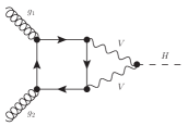
(a)

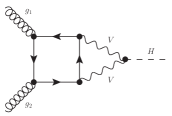
(b)

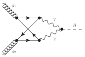
(c)

Figure 1: The two-loop light-quark electroweak contributions to $gg\to H$. $V$ stands for $W^{\pm},Z$ and the fermionic lines represent different quarks, depending on the electroweak boson $V$.

Thanks to gauge-invariance and parity constraints, the $gg\to H$ scattering amplitude is expressed in terms of a single form factor

$$\mathcal{M}^{c_{1}c_{2}}_{\lambda_{1}\lambda_{2}}=\mathcal{F}\left(s,m_{W}^{2},m_{Z}^{2}\right)\left[\eta_{\mu\nu}-\frac{p_{2\mu}p_{1\nu}}{p_{1}\cdot p_{2}}\right]\delta^{c_{1}c_{2}}\varepsilon_{\lambda_{1}}^{\mu}(\mathbf{p}_{1})\varepsilon_{\lambda_{2}}^{\nu}(\mathbf{p}_{2}).$$ (2.1)

It is possible to extract the form factor $\mathcal{F}$ by contracting $\mathcal{M}_{\lambda_{1}\lambda_{2}}^{c_{1}c_{2}}$ with the projection operator

$$\mathbb{P}_{c_{1}c_{2}}^{\lambda_{1}\lambda_{2}}=\varepsilon^{*\lambda_{1}}_{\mu}(\mathbf{p}_{1})\varepsilon^{*\lambda_{2}}_{\nu}(\mathbf{p}_{2})\frac{\delta_{c_{1}c_{2}}}{N_{c}^{2}-1}\frac{1}{d-2}\left[\eta^{\mu\nu}-\frac{p_{1}^{\mu}p_{2}^{\nu}+p_{1}^{\nu}p_{2}^{\mu}}{p_{1}\cdot p_{2}}\right].$$ (2.2)

We find

$$\mathcal{F}\left(s,m_{W}^{2},m_{Z}^{2}\right)=\sum_{\lambda_{1},\lambda_{2},c_{1},c_{2}}\mathbb{P}_{c_{1},c_{2}}^{\lambda_{1}\lambda_{2}}\mathcal{M}_{\lambda_{1}\lambda_{2}}^{c_{1},c_{2}}.$$ (2.3)

The form factor $\mathcal{F}$ is a linear combination of integrals which depend on the scalar products between loop and external momenta, and on the scalar products of loop momenta between themselves. All the integrals in $\mathcal{F}$ are obtained starting from the two topologies shown in Figure 2. At variance with Feynman diagrams in Figure 1, when we consider topologies and master integrals, we use wavy (solid) lines to denote massless (massive) propagators, respectively. We take all momenta to be incoming, i.e.

$$p_{3}=-p_{1}-p_{2},\;\;\;p_{1,2}^{2}=0,\;\;\;\;p_{3}^{3}=s=m_{H}^{2}.$$ (2.4)

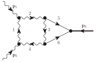
(a)

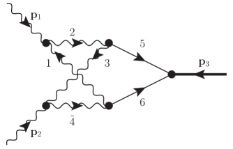
(b)

Figure 2: Planar (left) and non-planar (right) topologies. See text for momenta assignments and propagator labels.

The planar and non-planar integrals are parametrized as

$$I_{\textup{P}}(a_{1},a_{2},a_{3},a_{4},a_{5},a_{6},a_{7}) =\int\frac{{\rm d}^{d}k_{1}{\rm d}^{d}k_{2}}{[\mathrm{i}\mathrm{\pi}^{2}\Gamma(1+\varepsilon)]^{2}}\frac{1}{[1]^{a_{1}}[2]^{a_{2}}[3]^{a_{3}}[4]^{a_{4}}[5]^{a_{5}}[6]^{a_{6}}[7]^{a_{7}}},$$ (2.5)

$$I_{\textup{NP}}(a_{1},a_{2},a_{3},a_{\tilde{4}},a_{5},a_{6},a_{7}) =\int\frac{{\rm d}^{d}k_{1}{\rm d}^{d}k_{2}}{[\mathrm{i}\mathrm{\pi}^{2}\Gamma(1+\varepsilon)]^{2}}\frac{1}{[1]^{a_{1}}[2]^{a_{2}}[3]^{a_{3}}[\tilde{4}]^{a_{\tilde{4}}}[5]^{a_{5}}[6]^{a_{6}}[7]^{a_{7}}},$$ (2.6)

where

$$\begin{split}&[1]=k_{1}^{2},\quad[2]=(k_{1}+p_{1})^{2},\quad[3]=k_{2}^{2},\quad[4]=(k_{1}-p_{2})^{2},\quad[\tilde{4}]=(k_{2}+p_{2})^{2},\\ &[5]=(k_{1}-k_{2}+p_{1})^{2}-M^{2},\quad[6]=(k_{2}-k_{1}+p_{2})^{2}-M^{2},\quad[7]=(k_{1}+k_{2})^{2}.\end{split}$$ (2.7)

In both cases, the propagator $[7]$ is auxiliary; it is only needed for the parametrization of tensor integrals with (otherwise) irreducible numerators. Both planar and non-planar integrals are analytic functions in the complex plane of the variable $s$ with the cut along the real axis starting at $s=0$. This discontinuity corresponds to massless intermediate states in Feynman diagrams. At $s\geq 4M^{2}$, it also becomes possible to produce pairs of vector bosons on the mass shell; this leads to additional contributions to the discontinuities of $I_{\textup{P,NP}}$. We use the program Reduze2 [16] to express all integrals that appear in the evaluation of $gg\to H$ amplitude through master integrals (MIs). We also use the integration-by-parts reduction identities to derive the differential equations in $s$ and $M^{2}$ satisfied by the master integrals.

3 Differential equations

We denote a vector of master integrals by ${\bf I}$, a set of kinematic variables by ${\bf x}\in\{s,M^{2}\}$, and write the differential equations as

$$\frac{\partial\mathbf{I}(\mathbf{x},\varepsilon)}{\partial\mathbf{x}_{i}}={\cal A}_{i}(\mathbf{x},\varepsilon)\mathbf{I}(\mathbf{x},\varepsilon).$$ (3.1)

It was conjectured in Ref. [11] that in many physically relevant cases a canonical basis of master integrals ${\bf I^{\prime}}$ exists with the property that the right hand side of the differential equation has a simple, factorized dependence on the regularization parameter $\varepsilon$. While the statement has not been rigorously proved, it is expected to be true at least for those cases that can be expressed in terms of Chen iterated integrals. The differential equations for the canonical basis assume the following form

$$\frac{\partial\mathbf{I}^{\prime}(\mathbf{x},\varepsilon)}{\partial\mathbf{x}_{i}}=\varepsilon\mathcal{A}^{\prime}_{i}(\mathbf{x})\mathbf{I}^{\prime}(\mathbf{x},\varepsilon),$$ (3.2)

so that the iterative construction of ${\bf I}^{\prime}$ as series in $\varepsilon$ becomes straightforward. General criteria to find candidate canonical integrals are given in Ref. [17] and, under certain conditions for ordinary differential equations, in Ref. [18]. We do not use this last algorithm in this paper; instead, we begin by constructing canonical bases for the simplest integrals in the set and gradually move to more complex ones, as described extensively in [19]. Since the original matrices $\mathcal{A}_{i}$ are relatively sparse, this approach turns out to be quite practical for finding the canonical basis.

It is convenient to choose as independent variables the center of mass energy squared $s$ and the dimensionless ratio $\omega=-M^{2}/s$. Since the dependence of any master integral on $s$ follows uniquely from its mass dimension, we write master integrals as

$$\mathbf{I}(s,\omega)=s^{-a-2\varepsilon}\;\mathcal{I}(\omega),$$ (3.3)

where $a$ is an integer determined by the canonical mass dimension of the integral. The non-trivial information is contained in the functions $\mathcal{I}_{i}(\omega)$, which are dimensionless quantities. By choosing these functions to be appropriately re-scaled versions of the master integrals found by Reduze2

$$\begin{array}[]{cc}\mathcal{I}_{1}(\omega)=\varepsilon^{2}(\varepsilon-1)(-s)^{2\varepsilon}\vbox{\hbox{\includegraphics[height=30.1388pt]{0bubble}}}&\mathcal{I}_{2}(\omega)=-\varepsilon^{2}(-s)^{2\varepsilon+1}(\omega+1)\vbox{\hbox{\includegraphics[height=30.1388pt]{sbubble1}}}\\ \mathcal{I}_{3}(\omega)=-\varepsilon^{2}(-s)^{2\varepsilon+1}(\omega+1)\vbox{\hbox{\includegraphics[height=30.1388pt]{sbubble2}}}&\mathcal{I}_{4}(\omega)=\varepsilon^{3}(-s)^{2\varepsilon+1}\vbox{\hbox{\includegraphics[height=30.1388pt]{Triangle1}}}\\ \mathcal{I}_{5}(\omega)=\varepsilon^{2}(-s)^{2\varepsilon+2}\omega\vbox{\hbox{\includegraphics[height=30.1388pt]{Triangle2}}}&\mathcal{I}_{6}(\omega)=-\varepsilon^{2}(-s)^{2\varepsilon+2}\vbox{\hbox{\includegraphics[height=30.1388pt]{Inclusion}}}\\ \mathcal{I}_{7}(\omega)=\varepsilon^{4}(-s)^{2\varepsilon+1}\vbox{\hbox{\includegraphics[height=30.1388pt]{DoubleTriangle}}}&\mathcal{I}_{8}(\omega)=\varepsilon^{4}(-s)^{2\varepsilon+1}\vbox{\hbox{\includegraphics[height=30.1388pt]{Arrow}}}\\ \mathcal{I}_{9}(\omega)=\varepsilon^{4}(-s)^{2\varepsilon+2}(4\omega+1)\vbox{\hbox{\includegraphics[height=30.1388pt]{NonPlanar}}}&\mathcal{I}_{10}(\omega)=\varepsilon^{2}(-s)^{2\varepsilon+1}\vbox{\hbox{\includegraphics[height=30.1388pt]{btadpole}}}\\ \mathcal{I}_{11}(\omega)=-\varepsilon^{2}(-s)^{2\varepsilon+2}\vbox{\hbox{\includegraphics[height=30.1388pt]{doublebubble}}}&\mathcal{I}_{12}(\omega)=-\varepsilon^{2}(1-2\varepsilon)(-s)^{2\varepsilon+2}\omega\vbox{\hbox{\includegraphics[height=30.1388pt]{Kite}}},\end{array}$$ (3.4)

we can cast the system of differential equations for ${\cal I}(\omega)$ in the following form

$$\frac{\mathrm{d}\mathcal{I}(\omega)}{\mathrm{d}\omega}=\left[\mathcal{A}_{0}(\omega)+\varepsilon\mathcal{A}_{1}(\omega)\right]\mathcal{I}(\omega).$$ (3.5)

The matrices ${\cal A}_{0,1}$ are rational functions of $\omega$, and have a block-triangular structure.

To construct a systematic expansion of master integrals in $\varepsilon$, it is convenient to change basis of master integrals and transform the system of differential equations into a canonical form. This requires $\mathcal{A}_{0}$ to be removed. We can do that in a symbolic form by first solving the matrix differential equation

$$\frac{\mathrm{d}\hat{S}_{\mathcal{A}_{0}}}{\mathrm{d}\omega}=\mathcal{A}_{0}(\omega)\hat{S}_{\mathcal{A}_{0}}\;\;\;\;\rightarrow\;\;\;\;\hat{S}_{\mathcal{A}_{0}}=P_{\omega}e^{\int\mathcal{A}_{0}(\omega^{\prime})\,\mathrm{d}\omega^{\prime}},$$ (3.6)

where $P_{\omega}$ is the path-ordering operator defined as

$$P_{\omega}e^{\int A_{0}(\omega^{\prime})\,\mathrm{d}\omega^{\prime}}=\sum_{k=0}^{+\infty}\int_{\omega_{0}}^{\omega}\mathcal{A}_{0}(\omega_{1})\int_{\omega_{0}}^{\omega_{1}}\mathcal{A}_{0}(\omega_{2})\dots\int_{\omega_{0}}^{\omega_{k-1}}\mathcal{A}_{0}(\omega_{k})\,\mathrm{d}\omega_{k}\dots\mathrm{d}\omega_{2}\mathrm{d}\omega_{1}.$$ (3.7)

By defining a new set of master integrals

$$\mathcal{F}=\hat{S}_{\mathcal{A}_{0}}^{-1}\;{\mathcal{I}},$$ (3.8)

it is easy to see that ${\cal F}$ satisfies differential equations in the canonical form

$$\frac{\mathrm{d}\mathcal{F}(\omega)}{\mathrm{d}\omega}=\varepsilon\hat{S}_{\mathcal{A}_{0}}^{-1}\mathcal{A}_{1}\hat{S}_{\mathcal{A}_{0}}\mathcal{F}(\omega).$$ (3.9)

The non-trivial part of this procedure is to find the matrix $\hat{S}_{\mathcal{A}_{0}}$. A systematic way to do that, based on the Magnus exponentiation was suggested in Ref. [20]. Instead, we do that iteratively, using the sparse nature of the matrix ${\cal A}_{0}$ and considering different blocks of ${\mathcal{A}}_{0}$ separately. As an illustration, consider two integrals from the list of master integrals, ${\cal I}_{2}$ and ${\cal I}_{3}$. Neglecting the matrix ${\mathcal{A}}_{1}$, we find that they satisfy the system of coupled differential equations

$$\frac{\mathrm{d}}{\mathrm{d}\omega}\begin{pmatrix}{\cal I}_{2}\\ {\cal I}_{3}\end{pmatrix}=\frac{1}{\omega+1}\begin{pmatrix}0&\,\,&-2\\ 0&\,\,&1\\ \end{pmatrix}\begin{pmatrix}{\cal I}_{2}\\ {\cal I}_{3}\end{pmatrix}.$$ (3.10)

Integrating this equation, we find

$$\begin{pmatrix}{\cal I}_{2}\\ {\cal I}_{3}\end{pmatrix}=\hat{S}_{0}\begin{pmatrix}\mathcal{C}_{1}\\ \mathcal{C}_{2}\\ \end{pmatrix},\;\;\;\hat{S}_{0}=\begin{pmatrix}-1&\,\,&-2\omega\\ 0&\,\,&\omega+1\\ \end{pmatrix},$$ (3.11)

where $\mathcal{C}_{1,2}$ are the two integration constants. Since the above solution satisfies the system of differential equations for arbitrary $\mathcal{C}_{1}$, $\mathcal{C}_{2}$, the matrix $\hat{S}_{0}$ satisfies the original differential equation

$$\frac{\mathrm{d}\hat{S}_{0}}{\mathrm{d}\omega}=\frac{1}{\omega+1}\begin{pmatrix}0&\,\,&-2\\ 0&\,\,&1\\ \end{pmatrix}\hat{S}_{0}$$ (3.12)

and, therefore, can be taken to be a part of $\hat{S}_{\mathcal{A}_{0}}$. Finally, we compute $\mathcal{F}=\hat{S}_{0}^{-1}\mathcal{I}$ and find

$$\mathcal{F}_{2}=-\mathcal{I}_{2}+\frac{2\omega}{1+\omega}\mathcal{I}_{3}=-\varepsilon^{2}(-s)^{2\varepsilon+1}\left[(\omega+1)\vbox{\hbox{\includegraphics[height=30.1388pt]{sbubble1}}}+2\omega\vbox{\hbox{\includegraphics[height=30.1388pt]{sbubble2}}}\right],$$

$$\mathcal{F}_{3}=\frac{1}{1+\omega}\mathcal{I}_{3}=\varepsilon^{2}(-s)^{2\varepsilon+1}\vbox{\hbox{\includegraphics[height=30.1388pt]{sbubble2}}}.$$

The system of differential equations for the integrals ${\cal F}_{2,3}$ is then guaranteed to be in the canonical form. We find

$$\frac{\mathrm{d}}{\mathrm{d}\omega}\begin{pmatrix}\mathcal{F}_{2}\\ \mathcal{F}_{3}\end{pmatrix}=\varepsilon\begin{pmatrix}-\frac{2}{\omega+1}&\,\,&\frac{4}{\omega+1}\\ \frac{1}{\omega+1}-\frac{1}{\omega}&\,\,&-\frac{2}{\omega+1}-\frac{1}{\omega}\\ \end{pmatrix}\begin{pmatrix}\mathcal{F}_{2}\\ \mathcal{F}_{3}\end{pmatrix},$$ (3.13)

We apply this procedure block by block, to the block-triangular matrix $\mathcal{A}_{0}+\varepsilon\mathcal{A}_{1}$ and obtain the canonical system of differential equations that we write in the following form

$$\mathrm{d}\mathcal{F}(\omega)=\varepsilon\,{\rm d}\mathcal{B}(\omega)\mathcal{F}(\omega).$$ (3.14)

The canonical basis of the master integrals $\mathcal{F}(\omega)$ reads

$$\tiny\begin{pmatrix}\varepsilon^{2}(\varepsilon-1)(-s)^{2\varepsilon}\vbox{\hbox{\includegraphics[height=15.0694pt]{0bubble}}}\\ -\varepsilon^{2}(-s)^{2\varepsilon+1}\left[(\omega+1)\vbox{\hbox{\includegraphics[height=15.0694pt]{sbubble1}}}+2\omega\vbox{\hbox{\includegraphics[height=15.0694pt]{sbubble2}}}\right]\\ \varepsilon^{2}(-s)^{2\varepsilon+1}\vbox{\hbox{\includegraphics[height=15.0694pt]{sbubble2}}}\\ \varepsilon^{3}(-s)^{2\varepsilon+1}\vbox{\hbox{\includegraphics[height=15.0694pt]{Triangle1}}}\\ \varepsilon^{2}\left[(1-\varepsilon)\frac{2}{\sqrt{1+4\omega}}(-s)^{2\varepsilon}\vbox{\hbox{\includegraphics[height=15.0694pt]{0bubble}}}+\varepsilon\frac{3(1+2\omega)}{\sqrt{1+4\omega}}(-s)^{2\varepsilon+1}\vbox{\hbox{\includegraphics[height=15.0694pt]{Triangle1}}}-(-s)^{2\varepsilon+2}\frac{\omega^{2}}{\sqrt{1+4\omega}}\vbox{\hbox{\includegraphics[height=15.0694pt]{Triangle2}}}\right]\\ \varepsilon^{2}\left[(1-\varepsilon)(-s)^{2\varepsilon}\frac{\sqrt{1+4\omega}}{2}\vbox{\hbox{\includegraphics[height=15.0694pt]{0bubble}}}+(-s)^{2\varepsilon+1}\frac{(\omega+1)\sqrt{1+4\omega}}{4}\vbox{\hbox{\includegraphics[height=15.0694pt]{sbubble1}}}+(-s)^{2\varepsilon+1}\frac{(\omega+1)\sqrt{1+4\omega}}{2}\vbox{\hbox{\includegraphics[height=15.0694pt]{sbubble2}}}+(-s)^{2\varepsilon+2}\omega\sqrt{1+4\omega}\vbox{\hbox{\includegraphics[height=15.0694pt]{Inclusion}}}\right]\\ \varepsilon^{4}(-s)^{2\varepsilon+1}\vbox{\hbox{\includegraphics[height=15.0694pt]{DoubleTriangle}}}\\ \varepsilon^{4}(-s)^{2\varepsilon+1}\vbox{\hbox{\includegraphics[height=15.0694pt]{Arrow}}}\\ \varepsilon^{4}(-s)^{2\varepsilon+2}\sqrt{4\omega+1}\vbox{\hbox{\includegraphics[height=15.0694pt]{NonPlanar}}}\\ \varepsilon^{2}(-s)^{2\varepsilon+1}\vbox{\hbox{\includegraphics[height=15.0694pt]{btadpole}}}\\ -\varepsilon^{2}(-s)^{2\varepsilon+2}\sqrt{4\omega+1}\vbox{\hbox{\includegraphics[height=15.0694pt]{doublebubble}}}\\ \varepsilon^{2}\left[\frac{1-\varepsilon}{2}(-s)^{2\varepsilon}\vbox{\hbox{\includegraphics[height=15.0694pt]{0bubble}}}+(-s)^{2\varepsilon+1}\frac{\omega+1}{4}\vbox{\hbox{\includegraphics[height=15.0694pt]{sbubble1}}}+(-s)^{2\varepsilon+1}\frac{\omega+1}{2}\vbox{\hbox{\includegraphics[height=15.0694pt]{sbubble2}}}+(-s)^{2\varepsilon+2}\omega\vbox{\hbox{\includegraphics[height=15.0694pt]{Inclusion}}}+(-s)^{2\varepsilon+2}\vbox{\hbox{\includegraphics[height=15.0694pt]{doublebubble}}}+(1-2\varepsilon)(-s)^{2\varepsilon+2}\omega\vbox{\hbox{\includegraphics[height=15.0694pt]{Kite}}}\right]\\ \end{pmatrix}.$$

For the matrix $\mathcal{B}(\omega)$ we obtain

$$\mathcal{B}(\omega)=B_{1}\,\log\omega+B_{2}\,\log(1+\omega)+\\ +B_{3}\,[\log(-1+\sqrt{1+4\omega})-\log(1+\sqrt{1+4\omega})]+B_{4}\,\log(1+4\omega).$$ (3.15)

The $\omega$-independent matrix coefficients in the above equation are given by

$$\tiny B_{1}=\setcounter{MaxMatrixCols}{12}\begin{pmatrix}-2&0&0&0&0&0&0&0&0&0&0&0\\ 0&0&0&0&0&0&0&0&0&0&0&0\\ 0&-1&-1&0&0&0&0&0&0&0&0&0\\ 0&0&0&-3&0&0&0&0&0&0&0&0\\ 0&0&0&0&-1&0&0&0&0&0&0&0\\ 0&0&0&0&0&-1&0&0&0&0&0&0\\ \frac{1}{2}&\frac{1}{4}&\frac{1}{2}&-\frac{1}{2}&0&0&-2&0&0&0&0&0\\ -1&-\frac{1}{2}&0&0&0&0&0&-2&0&0&0&0\\ 0&0&0&0&0&0&0&0&0&0&0&0\\ 0&0&0&0&0&0&0&0&0&-1&0&0\\ 0&0&0&0&0&0&0&0&0&0&0&0\\ 1&\frac{1}{2}&\frac{1}{2}&0&0&0&0&0&0&0&0&-2\\ \end{pmatrix},\quad\tiny B_{2}=\setcounter{MaxMatrixCols}{12}\begin{pmatrix}0&0&0&0&0&0&0&0&0&0&0&0\\ 0&-2&4&0&0&0&0&0&0&0&0&0\\ 0&1&-2&0&0&0&0&0&0&0&0&0\\ 0&0&0&0&0&0&0&0&0&0&0&0\\ 0&0&0&0&0&0&0&0&0&0&0&0\\ 0&0&0&0&0&0&0&0&0&0&0&0\\ 0&0&0&0&0&0&0&0&0&0&0&0\\ 0&0&0&0&0&0&0&0&0&0&0&0\\ 0&0&0&0&0&0&0&0&0&0&0&0\\ 0&0&0&0&0&0&0&0&0&0&0&0\\ 0&0&0&0&0&0&0&0&0&0&0&0\\ 0&0&0&0&0&0&0&0&0&0&0&0\\ \end{pmatrix},$$ (3.16)

$$\tiny B_{3}=\setcounter{MaxMatrixCols}{12}\begin{pmatrix}0&0&0&0&0&0&0&0&0&0&0&0\\ 0&0&0&0&0&0&0&0&0&0&0&0\\ 0&0&0&0&0&0&0&0&0&0&0&0\\ 0&0&0&0&1&0&0&0&0&0&0&0\\ -4&0&0&3&0&0&0&0&0&0&0&0\\ \frac{1}{2}&-\frac{3}{4}&0&0&0&0&0&0&0&0&0&0\\ 0&0&0&0&-\frac{1}{2}&-1&0&0&0&0&0&0\\ 0&0&0&0&0&0&0&0&0&0&0&0\\ 6&3&0&-8&0&0&-8&4&0&0&0&0\\ 0&0&0&0&0&0&0&0&0&0&0&0\\ 0&0&0&0&0&0&0&0&0&-1&0&0\\ 0&0&0&0&0&2&0&0&0&0&-2&0\\ \end{pmatrix},\quad\tiny B_{4}=\setcounter{MaxMatrixCols}{12}\begin{pmatrix}0&0&0&0&0&0&0&0&0&0&0&0\\ 0&0&0&0&0&0&0&0&0&0&0&0\\ 0&0&0&0&0&0&0&0&0&0&0&0\\ 0&0&0&0&0&0&0&0&0&0&0&0\\ 0&0&0&0&-1&0&0&0&0&0&0&0\\ 0&0&0&0&0&-1&0&0&0&0&0&0\\ 0&0&0&0&0&0&0&0&0&0&0&0\\ 0&0&0&0&0&0&0&0&0&0&0&0\\ 0&0&0&0&0&0&0&0&-2&0&0&0\\ 0&0&0&0&0&0&0&0&0&0&0&0\\ 0&0&0&0&0&0&0&0&0&0&-1&0\\ 0&0&0&0&0&0&0&0&0&0&0&0\\ \end{pmatrix}.$$ (3.17)

It is convenient to remove the square roots from the Eqs. (3.14,3.15) by changing variables $\omega\to y$ where

$$y=\frac{\sqrt{1+4\omega}-1}{\sqrt{1+4\omega}+1}.$$ (3.18)

The differential equations (3.14) take the following form

$$\mathrm{d}\mathcal{F}(y)=\varepsilon\,{\rm d}\mathcal{C}(y)\mathcal{F}(y),$$ (3.19)

where the matrix $\mathcal{C}$ reads

$$\mathcal{C}(y)=C_{1}\,\log y+C_{2}\,\log(1-y)+C_{3}\,\log(1+y)+C_{4}\,\log(1-y+y^{2}).$$ (3.20)

The $y$-independent matrices $C_{1,\dots,4}$ are

$$\tiny C_{1}=\setcounter{MaxMatrixCols}{12}\begin{pmatrix}-2&0&0&0&0&0&0&0&0&0&0&0\\ 0&0&0&0&0&0&0&0&0&0&0&0\\ 0&-1&-1&0&0&0&0&0&0&0&0&0\\ 0&0&0&-3&1&0&0&0&0&0&0&0\\ -4&0&0&3&-1&0&0&0&0&0&0&0\\ \frac{1}{2}&-\frac{3}{4}&0&0&0&-1&0&0&0&0&0&0\\ \frac{1}{2}&\frac{1}{4}&\frac{1}{2}&-\frac{1}{2}&-\frac{1}{2}&-1&-2&0&0&0&0&0\\ -1&-\frac{1}{2}&0&0&0&0&0&-2&0&0&0&0\\ 6&3&0&-8&0&0&-8&4&0&0&0&0\\ 0&0&0&0&0&0&0&0&0&-1&0&0\\ 0&0&0&0&0&0&0&0&0&-1&0&0\\ 1&\frac{1}{2}&\frac{1}{2}&0&0&2&0&0&0&0&-2&-2\\ \end{pmatrix},\quad\tiny C_{2}=\setcounter{MaxMatrixCols}{12}\begin{pmatrix}4&0&0&0&0&0&0&0&0&0&0&0\\ 0&4&-8&0&0&0&0&0&0&0&0&0\\ 0&0&6&0&0&0&0&0&0&0&0&0\\ 0&0&0&6&0&0&0&0&0&0&0&0\\ 0&0&0&0&4&0&0&0&0&0&0&0\\ 0&0&0&0&0&4&0&0&0&0&0&0\\ -1&-\frac{1}{2}&-1&1&0&0&4&0&0&0&0&0\\ 2&1&0&0&0&0&0&4&0&0&0&0\\ 0&0&0&0&0&0&0&0&4&0&0&0\\ 0&0&0&0&0&0&0&0&0&2&0&0\\ 0&0&0&0&0&0&0&0&0&0&2&0\\ -2&-1&-1&0&0&0&0&0&0&0&0&4\\ \end{pmatrix},$$ (3.21)

$$\tiny C_{3}=\setcounter{MaxMatrixCols}{12}\begin{pmatrix}0&0&0&0&0&0&0&0&0&0&0&0\\ 0&0&0&0&0&0&0&0&0&0&0&0\\ 0&0&0&0&0&0&0&0&0&0&0&0\\ 0&0&0&0&0&0&0&0&0&0&0&0\\ 0&0&0&0&-2&0&0&0&0&0&0&0\\ 0&0&0&0&0&-2&0&0&0&0&0&0\\ 0&0&0&0&0&0&0&0&0&0&0&0\\ 0&0&0&0&0&0&0&0&0&0&0&0\\ 0&0&0&0&0&0&0&0&-4&0&0&0\\ 0&0&0&0&0&0&0&0&0&0&0&0\\ 0&0&0&0&0&0&0&0&0&0&-2&0\\ 0&0&0&0&0&0&0&0&0&0&0&0\\ \end{pmatrix},\quad\tiny C_{4}=\setcounter{MaxMatrixCols}{12}\begin{pmatrix}0&0&0&0&0&0&0&0&0&0&0&0\\ 0&-2&4&0&0&0&0&0&0&0&0&0\\ 0&1&-2&0&0&0&0&0&0&0&0&0\\ 0&0&0&0&0&0&0&0&0&0&0&0\\ 0&0&0&0&0&0&0&0&0&0&0&0\\ 0&0&0&0&0&0&0&0&0&0&0&0\\ 0&0&0&0&0&0&0&0&0&0&0&0\\ 0&0&0&0&0&0&0&0&0&0&0&0\\ 0&0&0&0&0&0&0&0&0&0&0&0\\ 0&0&0&0&0&0&0&0&0&0&0&0\\ 0&0&0&0&0&0&0&0&0&0&0&0\\ 0&0&0&0&0&0&0&0&0&0&0&0\\ \end{pmatrix}.$$ (3.22)

It is straightforward to write the solution of the system of differential equations (3.19) as Taylor series in $\varepsilon$

$$\begin{split}\mathcal{F}(y)&=\mathcal{F}_{0}^{(0)}+\varepsilon\left[\int_{0}^{y}\mathcal{C}(\tau_{1})\mathcal{F}_{0}^{(0)}\,\mathrm{d}\tau_{1}+\mathcal{F}_{0}^{(1)}\right]+\\ &+\varepsilon^{2}\left[\int_{0}^{y}\mathcal{C}(\tau_{1})\int_{0}^{\tau_{1}}\mathcal{C}(\tau_{2})\mathcal{F}_{0}^{(0)}\,\mathrm{d}\tau_{2}\mathrm{d}\tau_{1}+\int_{0}^{y}\mathcal{C}(\tau_{1})\mathcal{F}_{0}^{(1)}\,\mathrm{d}\tau_{1}+\mathcal{F}_{0}^{(2)}\right]+...,\end{split}$$ (3.23)

where $\mathcal{F}_{0}^{(i)}$ are integration constants that can not be fixed from the differential equations.

Given the iterative structure of the solution, it can be written as a linear combination of the so-called Goncharov’s polylogarithms (GPLs), also known as hyperlogarithms, defined as [14, 13, 21, 15]

$$G(m_{w},\mathbf{m}_{w-1};x):=\begin{cases}\frac{1}{w!}\log^{w}x&\text{if $\mathbf{m}_{w}=(0,\dots,0)$}\\ \int_{0}^{x}f(m_{w};\tau)\;G(\mathbf{m}_{w-1};\tau)\,\mathrm{d}\tau&\text{if $\mathbf{m}_{w}\neq(0,\dots,0)$}\end{cases},$$ (3.24)

where $\mathbf{m}_{w}$ indicates the vector $(m_{w},\mathbf{m}_{w-1})$. The functions $f(a;\tau)$ represent the integration kernels; for our system of differential equations they span the following set

$$f(0;\tau)=\frac{1}{\tau},\quad f(1;\tau)=\frac{1}{\tau-1},\quad f(-1;\tau)=\frac{1}{\tau+1},\quad f(r;\tau)=\frac{2\tau-1}{\tau^{2}-\tau+1}.$$ (3.25)

The last term in the set is quadratic in the integration variable; it is possible to re-write it in a usual linear form

$$f(r;\tau)=\frac{2\tau-1}{\tau^{2}-\tau+1}=\frac{1}{\tau-r_{+}}+\frac{1}{\tau-r_{-}}=f(r_{+};\tau)+f(r_{-};\tau),\;\;\;\;r_{\pm}=\mathrm{e}^{\pm\mathrm{i}\frac{\mathrm{\pi}}{3}},$$ (3.26)

at the expense of introducing complex-valued poles. This last step is essential for numerical evaluation of the GPLs but it is not required to integrate the system of differential equations since, thanks to the linearity of the differential equations and the definition of the GPLs,

$$G(\dots,r,\dots;x)=G(\dots,r_{-},\dots;x)+G(\dots,r_{+},\dots;x).$$ (3.27)

This implies that we can perform the analytic integration using the symbol $r$ and then, for the numerical evaluation of the final result, switch to $r_{\pm}$ using Eq. (3.27).

In Table 1 the relations among $s$, $\omega$ and $y$, as well as the different kinematic regions, are summarized.

Variable	Euclidean	Minkowski, below threshold	Above threshold
$s$	$-\infty<s<0$	$0<s<4M^{2}$	$4M^{2}<s<+\infty$
$\omega=-\frac{M^{2}}{s}$	$0<\omega<+\infty$	$-\infty<\omega<-\frac{1}{4}$	$-\frac{1}{4}<\omega<0$
$y=\frac{\sqrt{1+4\omega}-1}{\sqrt{1+4\omega}+1}$	$0<y<1$	$\mathrm{e}^{\mathrm{i}\vartheta}$, $0<\vartheta<\mathrm{\pi}$	$-1<y<0$

Table 1: Different kinematic regions in $s$, $\omega$ and $y$.

4 Boundary conditions and analytic continuation

Linear differential equations allow us to restore the dependencies of master integrals on $\omega$ up to a single constant. The constant can be fixed by computing the required integral at any point $\omega=\omega_{0}$ and comparing the result with the solution of the differential equation.

It turns out to be convenient to determine the boundary conditions by computing the master integrals in $\omega\to\infty$ or $y\to 1$ limit. Since $\omega=-M^{2}/s$, this corresponds to $M^{2}\to\infty$ at fixed $s$; in this limit the integrals can be easily computed using the so-called large-mass expansion procedure [24]. The large-mass expansion procedure can be formulated as follows: consider two different scalings for each of the loop momenta $k_{1,2}\sim M$ and $k_{1,2}\sim\sqrt{s}$ and, for a chosen scaling, systematically expand the integrand in Taylor series in all small variables. The set of small variables will differ from scaling to scaling; for example, if $k_{1}\sim k_{2}\sim M$, one Taylor expands in external momenta but if the scaling $k_{1}\sim M$, $k_{2}\sim\sqrt{s}$ is considered, one Taylor expands in the external momenta and $k_{2}$. It is easy to see that, to leading order in $s/M^{2}$, most of the master integrals are expressed in terms of two-loop tadpole integrals and, in some cases, in terms of products of one-loop three- and two-point integrals and one-loop tadpole integrals.

As an illustration, consider the non-planar master integral

$${\cal F}_{9}(\omega)=\varepsilon^{4}(-s)^{2\varepsilon+2}\sqrt{4\omega+1}\vbox{\hbox{\includegraphics[height=30.1388pt]{NonPlanar}}}.$$ (4.1)

We are interested in determining its behavior in the $y\to 1$ limit. By applying the large mass expansion, we find that the non-planar integral scales as

$$\lim_{M\gg\sqrt{s}}\vbox{\hbox{\includegraphics[height=30.1388pt]{NonPlanar}}}=\vbox{\hbox{\includegraphics[height=30.1388pt]{G5}}}={\cal O}\left(M^{-4}\right)$$ (4.2)

in the large-$M$ limit. This implies that the large-$M$ limit of the $\mathcal{F}_{9}$ non-planar master integral reads

$${\cal F}_{9}(\omega)\sim\frac{\varepsilon^{4}(-s)^{2\varepsilon+2}\sqrt{4\omega+1}}{M^{4}}\sim\frac{1}{\omega^{3/2}}\sim(1-y)^{3},$$ (4.3)

where we used relations among $s$, $\omega$ and $y$ variables summarized in Table 1. $\mathcal{F}_{9}$ vanishes as $(1-y)^{3}$ as $y$ goes to $1$, and this information is sufficient to fix the constant of integration for this master integral.

A similar analysis reveals that only three master integrals ${\cal F}_{1},{\cal F}_{2},{\cal F}_{10}$ possess non-vanishing $y\to 1$ limit. These limits are

$$\lim_{y\to 1}\mathcal{F}_{1}(y) =-(1-y)^{4\varepsilon}\frac{\Gamma(1+2\varepsilon)\Gamma(1-\varepsilon)}{2\Gamma(\varepsilon+1)},$$ (4.4)

$$\lim_{y\to 1}\mathcal{F}_{2}(y) =(1-y)^{4\varepsilon}\frac{\Gamma(1+2\varepsilon)\Gamma(1-\varepsilon)}{\Gamma(\varepsilon+1)},$$ (4.5)

$$\lim_{y\to 1}\mathcal{F}_{10}(y) =(1-y)^{4\varepsilon}\frac{\Gamma^{2}(1-\varepsilon)}{\Gamma(1-2\varepsilon)}.$$ (4.6)

To fix the boundary conditions, we need to evaluate the GPLs of the form $G(\mathbf{m},y)$, where $\mathbf{m}$ is composed of the elements of the set

$$\{\quad 0,\quad 1,\quad-1,\quad\mathrm{e}^{\mathrm{i}\frac{\mathrm{\pi}}{3}},\quad\mathrm{e}^{-\mathrm{i}\frac{\mathrm{\pi}}{3}}\quad\},$$ (4.7)

and the limit $y\to 1$ is taken where possible. For weights higher than three, not all the Goncharov polylogarithms at $y=1$ with the arguments from Eq. (4.7) can be analytically expressed in terms of canonical irrational numbers such as $\pi$ and $\zeta(n)$. Nevertheless, we expect that the boundary constants are linear combinations of these irrational numbers; to find them we follow a numerical approach. We use our solution of the differential equations and the boundary conditions discussed above to find the integration constants numerically with high precision. We then fit the resulting numerical value to a linear combination of $\pi^{2}$ and $\zeta(n)$ of a well-defined weight. For example, at weight two we only have $\pi^{2}$, at weight three $\zeta(3)$, at weight four $\pi^{4}$, at weight five $\zeta(5)$ and $\pi^{2}\zeta(3)$ and at weight six $\pi^{6}$ and $\zeta(3)^{2}$. For each of the master integrals, we have achieved the matching of the numerical and the analytic results to at least 750 digits.

Our final remark concerns the analytic continuation of the master integrals $\mathcal{F}(y)$. So far, we have studied them in the Euclidean region but we need them in the region where $s=m_{H}^{2}>0$ and, yet, $s<4M^{2}$. The correct analytic continuation is achieved by replacing $s\to s+\mathrm{i}0$ at fixed $M^{2}$. It is easy to see that this implies $\omega\to\omega+\mathrm{i}0$ and $y\to y+\mathrm{i}0$.

All the master integrals evaluated here have been compared for at least four different values of $s/M^{2}$, both in the Euclidean and Minkowski region, to the numerical results obtained with the program Secdec [25]. In all cases we found excellent agreement.

5 Form factor for $gg\to H$

The $gg\to H$ amplitude is described by a single form factor, as explained in Section 2. This form factor receives contributions from loops with $W$ and $Z$ bosons. The form factor is finite in four dimensions ($\varepsilon\to 0$) and can be written as:

$$\mathcal{F}(s,m_{W}^{2},m_{Z}^{2})=-(4\mathrm{\pi})^{4\varepsilon}(-s)^{2\varepsilon}\Gamma^{2}(\varepsilon+1)\\ \times\frac{\mathrm{i}\alpha_{S}\alpha^{2}}{4\mathrm{\pi}\sin^{4}\vartheta_{W}}\frac{v}{2}\left[4\mathcal{A}(y_{W})+\frac{2}{\cos^{4}\vartheta_{W}}\left(\frac{5}{4}-\frac{7}{3}\sin^{2}\vartheta_{W}+\frac{22}{9}\sin^{4}\vartheta_{W}\right)\mathcal{A}(y_{Z})\right],$$ (5.1)

where

$$y_{W}=\frac{\sqrt{1-4m_{W}^{2}/m_{H}^{2}}-1}{\sqrt{1-4m_{W}^{2}/m_{H}^{2}}+1},\qquad y_{Z}=\frac{\sqrt{1-4m_{Z}^{2}/m_{H}^{2}}-1}{\sqrt{1-4m_{Z}^{2}/m_{H}^{2}}+1}.$$ (5.2)

We take the CKM matrix to be an identity matrix. The contributions of $W$ bosons is computed in Eq. (5.1) taking into account first and second generations. The contribution of the $Z$ boson is calculated for five massless quarks ($u$, $d$, $s$, $c$ and $b$).

The function $\mathcal{A}$ in Eq. (5.1) can be expanded in $\varepsilon$; we have computed it through $\mathcal{O}\left(\varepsilon^{2}\right)$:

$$\mathcal{A}(y)=\mathcal{A}_{0}(y)+\varepsilon\mathcal{A}_{1}(y)+\varepsilon^{2}\mathcal{A}_{2}(y)+\mathcal{O}\left(\varepsilon^{3}\right).$$ (5.3)

The function $\mathcal{A}_{0}(y)$ reads

$$\begin{split}&\mathcal{A}_{0}(y)=\frac{1}{6(y-1)^{3}}\left[-6-6y(y^{2}-y+2)G(0,0,r,y)-6(1-y)(y^{2}-y+1)G(r,y)\right.\\ &\left.+(y+1)(y^{2}+1)[18G(-1,0,r,y)+\mathrm{\pi}^{2}G(-1,y)-18G(-1,0,0,y)]\right.\\ &\left.+12y(2y^{2}+y+1)[G(0,1,0,y)-G(0,1,r,y)]\right.\\ &\left.+2(1-y)(y^{2}+y+1)[6G(1,0,r,y)-12G(1,1,r,y)-\mathrm{\pi}^{2}G(1,y)+12G(1,1,0,y)]\right.\\ &\left.+6y(1-y)[G(0,r,y)-2G(1,r,y)+G(0,0,y)-2G(1,0,y)]\right.\\ &\left.-6y^{2}(y+1)G(0,0,0,y)-y(3\mathrm{\pi}^{2}y^{2}+12y^{2}+\mathrm{\pi}^{2}y-18y+2\mathrm{\pi}^{2}+6)G(0,y)\right.\\ &\left.-12(1-y)(2y^{2}+y+2)G(1,0,0,y)-6(y+3)(y^{2}+1)\zeta(3)\right.\\ &\left.+(1-y)(12y^{2}-\mathrm{\pi}^{2}y-24y+12)\right].\end{split}$$ (5.4)

We see that, although $\mathcal{A}_{0}$ is the finite part of a 2-loop form factor, the highest weight of the GPLs that appears in Eq. (5.1) is three. This happens because none of the master integrals that have $1/\varepsilon^{4}$ poles contribute to the $gg\to H$ amplitude at leading order in the $\varepsilon\to 0$ limit.

The expression for $\mathcal{F}$ in Eq. (5.1) has been compared with a previous calculation in Ref. [4] and agreement was found. The terms $\mathcal{A}_{1}(y)$ and $\mathcal{A}_{2}(y)$ are new. They can be found in the ancillary file provided with this paper.

6 Conclusions

We have presented a calculation of the mixed two-loop QCD-electroweak corrections mediated by massless quarks to the production of the Higgs boson in gluon fusion. We extended the known result for these corrections to two higher orders in the dimensional regularization parameter $\varepsilon$. This is one of the ingredients required for the computation of the NLO mixed QCD-electroweak corrections to $gg\to H$ amplitudes. We employed the method of differential equations, determined a canonical basis of master integrals and expressed all the relevant functions in terms of Goncharov polylogarithms. Finally, we used a mixed numerical and analytical approach, based on the PSLQ algorithm, in order to fix all necessary boundary conditions. This establishes the necessary framework to successfully address the calculation of the missing three-loop virtual contributions, whose calculation is ongoing.

Appendix A $\mathcal{F}_{0}$ values

In this appendix we present the boundary conditions for the master integrals defined in Eq. (3.23). The weights 0, 1 and 2 were determined analytically. For weights 4, 5 and 6 the results were obtained by fitting numerical results to an analytic Ansatz to at least 750 digits.

$$\mathcal{F}_{1}(y)=\varepsilon^{2}(\varepsilon-1)(-s)^{2\varepsilon}\vbox{\hbox{\includegraphics[height=30.1388pt]{0bubble}}}$$ (A.1)

$$\begin{split}\mathcal{F}_{0,1}^{(0)}=-\frac{1}{2},\quad\mathcal{F}_{0,1}^{(1)}=0,\quad\mathcal{F}_{0,1}^{(2)}=-\frac{\pi^{2}}{6},\quad\mathcal{F}_{0,1}^{(3)}=\zeta(3),\quad\\ \mathcal{F}_{0,1}^{(4)}=-\frac{\pi^{4}}{20},\quad\mathcal{F}_{0,1}^{(5)}=\frac{1}{3}\left[\pi^{2}\zeta(3)+9\zeta(5)\right],\quad\mathcal{F}_{0,1}^{(6)}=-\zeta^{2}(3)-\frac{61\pi^{6}}{3780}.\end{split}$$ (A.2)

$$\mathcal{F}_{2}(y)=-\varepsilon^{2}(-s)^{2\varepsilon+1}\left[(\omega+1)\vbox{\hbox{\includegraphics[height=30.1388pt]{sbubble1}}}+2\omega\vbox{\hbox{\includegraphics[height=30.1388pt]{sbubble2}}}\right]$$ (A.3)

$$\begin{split}\mathcal{F}_{0,2}^{(0)}=1,\quad\mathcal{F}_{0,2}^{(1)}=0,\quad\mathcal{F}_{0,2}^{(2)}=-\frac{\pi^{2}}{3},\quad\mathcal{F}_{0,2}^{(3)}=-10\zeta(3),\quad\\ \mathcal{F}_{0,2}^{(4)}=-\frac{11\pi^{4}}{90},\quad\mathcal{F}_{0,2}^{(5)}=\frac{10\pi^{2}\zeta(3)}{3}-54\zeta(5),\quad\mathcal{F}_{0,2}^{(6)}=50\zeta^{2}(3)-\frac{121\pi^{6}}{1890}.\end{split}$$ (A.4)

$$\mathcal{F}_{3}(y)=\varepsilon^{2}(-s)^{2\varepsilon+1}\vbox{\hbox{\includegraphics[height=30.1388pt]{sbubble2}}}$$ (A.5)

$$\begin{split}\mathcal{F}_{0,3}^{(0)}=0,\quad\mathcal{F}_{0,3}^{(1)}=0,\quad\mathcal{F}_{0,3}^{(2)}=\frac{\pi^{2}}{6},\quad\mathcal{F}_{0,3}^{(3)}=8\zeta(3),\quad\\ \mathcal{F}_{0,3}^{(4)}=\frac{7\pi^{4}}{72},\quad\mathcal{F}_{0,3}^{(5)}=48\zeta(5)-3\pi^{2}\zeta(3),\quad\mathcal{F}_{0,3}^{(6)}=\frac{127\pi^{6}}{2160}-48\zeta^{2}(3).\end{split}$$ (A.6)

$$\mathcal{F}_{4}(y)=\varepsilon^{3}(-s)^{2\varepsilon+1}\vbox{\hbox{\includegraphics[height=30.1388pt]{Triangle1}}}$$ (A.7)

$$\begin{split}\mathcal{F}_{0,4}^{(0)}=0,\quad\mathcal{F}_{0,4}^{(1)}=0,\quad\mathcal{F}_{0,4}^{(2)}=0,\quad\mathcal{F}_{0,4}^{(3)}=-2\zeta(3),\quad\\ \mathcal{F}_{0,4}^{(4)}=-\frac{\pi^{4}}{180},\quad\mathcal{F}_{0,4}^{(5)}=-\frac{\pi^{2}\zeta(3)}{3}-12\zeta(5),\quad\mathcal{F}_{0,4}^{(6)}=9\zeta^{2}(3)-\frac{37\pi^{6}}{3780}.\end{split}$$ (A.8)

$$\mathcal{F}_{5}(y)=\varepsilon^{2}\left[-2(\varepsilon-1)(-s)^{2\varepsilon}\vbox{\hbox{\includegraphics[height=30.1388pt]{0bubble}}}+\varepsilon\frac{3(1+2\omega)}{\sqrt{1+4\omega}}(-s)^{2\varepsilon+1}\vbox{\hbox{\includegraphics[height=30.1388pt]{Triangle1}}}+\right.\\ \left.-(-s)^{2\varepsilon+2}\frac{\omega^{2}}{\sqrt{1+4\omega}}\vbox{\hbox{\includegraphics[height=30.1388pt]{Triangle2}}}\right]$$ (A.9)

$$\begin{split}\mathcal{F}_{0,5}^{(0)}=0,\quad\mathcal{F}_{0,5}^{(1)}=0,\quad\mathcal{F}_{0,5}^{(2)}=-\frac{\pi^{2}}{3},\quad\mathcal{F}_{0,5}^{(3)}=-4\zeta(3),\quad\\ \mathcal{F}_{0,5}^{(4)}=-\frac{41\pi^{4}}{180},\quad\mathcal{F}_{0,5}^{(5)}=\pi^{2}\zeta(3)-30\zeta(5),\quad\mathcal{F}_{0,5}^{(6)}=21\zeta^{2}(3)-\frac{97\pi^{6}}{756}.\end{split}$$ (A.10)

$$\mathcal{F}_{6}(y)=\varepsilon^{2}\left[(1-\varepsilon)(-s)^{2\varepsilon}\frac{\sqrt{1+4\omega}}{2}\vbox{\hbox{\includegraphics[height=30.1388pt]{0bubble}}}+(-s)^{2\varepsilon+1}\frac{(\omega+1)\sqrt{1+4\omega}}{4}\vbox{\hbox{\includegraphics[height=30.1388pt]{sbubble1}}}+\right.\\ \left.+(-s)^{2\varepsilon+1}\frac{(\omega+1)\sqrt{1+4\omega}}{2}\vbox{\hbox{\includegraphics[height=30.1388pt]{sbubble2}}}+(-s)^{2\varepsilon+2}\omega\sqrt{1+4\omega}\vbox{\hbox{\includegraphics[height=30.1388pt]{Inclusion}}}\right]$$ (A.11)

$$\begin{split}\mathcal{F}_{0,6}^{(0)}=0,\quad\mathcal{F}_{0,6}^{(1)}=0,\quad\mathcal{F}_{0,6}^{(2)}=\frac{\pi^{2}}{4},\quad\mathcal{F}_{0,6}^{(3)}=6\zeta(3),\quad\\ \mathcal{F}_{0,6}^{(4)}=\frac{5\pi^{4}}{48},\quad\mathcal{F}_{0,6}^{(5)}=36\zeta(5)-\frac{5\pi^{2}\zeta(3)}{2},\quad\mathcal{F}_{0,6}^{(6)}=\frac{77\pi^{6}}{1440}-36\zeta^{2}(3).\end{split}$$ (A.12)

$$\mathcal{F}_{7}(y)=\varepsilon^{4}(-s)^{2\varepsilon+1}\vbox{\hbox{\includegraphics[height=30.1388pt]{DoubleTriangle}}}$$ (A.13)

$$\begin{split}\mathcal{F}_{0,7}^{(0)}=0,\quad\mathcal{F}_{0,7}^{(1)}=0,\quad\mathcal{F}_{0,7}^{(2)}=0,\quad\mathcal{F}_{0,7}^{(3)}=\zeta(3),\quad\\ \mathcal{F}_{0,7}^{(4)}=\frac{5\pi^{4}}{72},\quad\mathcal{F}_{0,7}^{(5)}=\frac{7\pi^{2}\zeta(3)}{6}+6\zeta(5),\quad\mathcal{F}_{0,7}^{(6)}=\frac{3\zeta^{2}(3)}{2}+\frac{13\pi^{6}}{270}.\end{split}$$ (A.14)

$$\mathcal{F}_{8}(y)=\varepsilon^{4}(-s)^{2\varepsilon+1}\vbox{\hbox{\includegraphics[height=30.1388pt]{Arrow}}}$$ (A.15)

$$\begin{split}\mathcal{F}_{0,8}^{(0)}=0,\quad\mathcal{F}_{0,8}^{(1)}=0,\quad\mathcal{F}_{0,8}^{(2)}=-\frac{\pi^{2}}{6},\quad\mathcal{F}_{0,8}^{(3)}=4\zeta(3),\quad\\ \mathcal{F}_{0,8}^{(4)}=-\frac{\pi^{4}}{9},\quad\mathcal{F}_{0,8}^{(5)}=\frac{\pi^{2}\zeta(3)}{3}+20\zeta(5),\quad\mathcal{F}_{0,8}^{(6)}=-16\zeta^{2}(3)-\frac{173\pi^{6}}{3780}.\end{split}$$ (A.16)

$$\mathcal{F}_{9}(y)=\varepsilon^{4}(-s)^{2\varepsilon+2}\sqrt{4\omega+1}\vbox{\hbox{\includegraphics[height=30.1388pt]{NonPlanar}}}$$ (A.17)

$$\begin{split}\mathcal{F}_{0,9}^{(0)}=0,\quad\mathcal{F}_{0,9}^{(1)}=0,\quad\mathcal{F}_{0,9}^{(2)}=-\frac{\pi^{2}}{3},\quad\mathcal{F}_{0,9}^{(3)}=-24\zeta(3),\quad\\ \mathcal{F}_{0,9}^{(4)}=\frac{13\pi^{4}}{45},\quad\mathcal{F}_{0,9}^{(5)}=\frac{46\pi^{2}\zeta(3)}{3}-100\zeta(5),\quad\mathcal{F}_{0,9}^{(6)}=264\zeta^{2}(3)+\frac{397\pi^{6}}{945}.\end{split}$$ (A.18)

$$\mathcal{F}_{10}(y)=\varepsilon^{2}(-s)^{2\varepsilon+1}\vbox{\hbox{\includegraphics[height=30.1388pt]{btadpole}}}$$ (A.19)

$$\begin{split}\mathcal{F}_{0,10}^{(0)}=1,\quad\mathcal{F}_{0,10}^{(1)}=0,\quad\mathcal{F}_{0,10}^{(2)}=-\frac{\pi^{2}}{6},\quad\mathcal{F}_{0,10}^{(3)}=-2\zeta(3),\quad\\ \mathcal{F}_{0,10}^{(4)}=-\frac{\pi^{4}}{40},\quad\mathcal{F}_{0,10}^{(5)}=\frac{\pi^{2}\zeta(3)}{3}-6\zeta(5),\quad\mathcal{F}_{0,10}^{(6)}=2\zeta^{2}(3)-\frac{79\pi^{6}}{15120}.\end{split}$$ (A.20)

$$\mathcal{F}_{11}(y)=-\varepsilon^{2}(-s)^{2\varepsilon+2}\sqrt{4\omega+1}\vbox{\hbox{\includegraphics[height=30.1388pt]{doublebubble}}}$$ (A.21)

$$\begin{split}\mathcal{F}_{0,11}^{(0)}=0,\quad\mathcal{F}_{0,11}^{(1)}=0,\quad\mathcal{F}_{0,11}^{(2)}=\frac{\pi^{2}}{6},\quad\mathcal{F}_{0,11}^{(3)}=2\zeta(3),\quad\\ \mathcal{F}_{0,11}^{(4)}=-\frac{\pi^{4}}{360},\quad\mathcal{F}_{0,11}^{(5)}=6\zeta(5)-\pi^{2}\zeta(3),\quad\mathcal{F}_{0,11}^{(6)}=-6\zeta^{2}(3)-\frac{47\pi^{6}}{15120}.\end{split}$$ (A.22)

$$\mathcal{F}_{12}(y)=\varepsilon^{2}\left[\frac{1-\varepsilon}{2}(-s)^{2\varepsilon}\vbox{\hbox{\includegraphics[height=30.1388pt]{0bubble}}}+(-s)^{2\varepsilon+1}\frac{\omega+1}{4}\vbox{\hbox{\includegraphics[height=30.1388pt]{sbubble1}}}+(-s)^{2\varepsilon+1}\frac{\omega+1}{2}\vbox{\hbox{\includegraphics[height=30.1388pt]{sbubble2}}}+\right.\\ \left.+(-s)^{2\varepsilon+2}\omega\vbox{\hbox{\includegraphics[height=30.1388pt]{Inclusion}}}+(-s)^{2\varepsilon+2}\vbox{\hbox{\includegraphics[height=30.1388pt]{doublebubble}}}+(1-2\varepsilon)(-s)^{2\varepsilon+2}\omega\vbox{\hbox{\includegraphics[height=30.1388pt]{Kite}}}\right]$$ (A.23)

$$\begin{split}\mathcal{F}_{0,12}^{(0)}=0,\quad\mathcal{F}_{0,12}^{(1)}=0,\quad\mathcal{F}_{0,12}^{(2)}=\frac{\pi^{2}}{12},\quad\mathcal{F}_{0,12}^{(3)}=4\zeta(3),\quad\\ \mathcal{F}_{0,12}^{(4)}=\frac{77\pi^{4}}{720},\quad\mathcal{F}_{0,12}^{(5)}=30\zeta(5)-\frac{3\pi^{2}\zeta(3)}{2},\quad\mathcal{F}_{0,12}^{(6)}=\frac{1711\pi^{6}}{30240}-30\zeta^{2}(3).\end{split}$$ (A.24)

References

• [1] C. Anastasiou, C. Duhr, F. Dulat, E. Furlan, T. Gehrmann, F. Herzog, A. Lazopoulos, and B. Mistlberger, High precision determination of the gluon fusion Higgs boson cross-section at the LHC, JHEP 05 (2016) 058, [arXiv:1602.0069].
• [2] C. Anastasiou, R. Boughezal, and F. Petriello, Mixed QCD-electroweak corrections to Higgs boson production in gluon fusion, JHEP 04 (2009) 003, [arXiv:0811.3458].
• [3] U. Aglietti, R. Bonciani, G. Degrassi, and A. Vicini, Two-loop electroweak corrections to Higgs production in proton-proton collisions, in TeV4LHC Workshop: 2nd Meeting Brookhaven, Upton, New York, February 3-5, 2005, 2006. hep-ph/0610033.
• [4] U. Aglietti, R. Bonciani, G. Degrassi, and A. Vicini, Two loop light fermion contribution to Higgs production and decays, Phys. Lett. B595 (2004) 432–441, [hep-ph/0404071].
• [5] U. Aglietti, R. Bonciani, G. Degrassi, and A. Vicini, Master integrals for the two-loop light fermion contributions to $gg\to H$ and $H\to\gamma\gamma$, Phys. Lett. B600 (2004) 57–64, [hep-ph/0407162].
• [6] S. Actis, G. Passarino, C. Sturm, and S. Uccirati, NNLO Computational Techniques: The Cases $H\to\gamma\gamma$ and $H\to gg$, Nucl. Phys. B811 (2009) 182–273, [arXiv:0809.3667].
• [7] S. Catani, The Singular behavior of QCD amplitudes at two loop order, Phys. Lett. B427 (1998) 161–171, [hep-ph/9802439].
• [8] A. V. Kotikov, Differential equations method: New technique for massive Feynman diagrams calculation, Phys. Lett. B254 (1991) 158–164.
• [9] E. Remiddi, Differential equations for Feynman graph amplitudes, Nuovo Cim. A110 (1997) 1435–1452, [hep-th/9711188].
• [10] T. Gehrmann and E. Remiddi, Differential equations for two loop four point functions, Nucl. Phys. B580 (2000) 485–518, [hep-ph/9912329].
• [11] J. M. Henn, Multiloop integrals in dimensional regularization made simple, Phys. Rev. Lett. 110 (2013) 251601, [arXiv:1304.1806].
• [12] C. G. Papadopoulos, Simplified differential equations approach for Master Integrals, JHEP 07 (2014) 088, [arXiv:1401.6057].
• [13] E. Remiddi and J. A. M. Vermaseren, Harmonic polylogarithms, Int. J. Mod. Phys. A15 (2000) 725–754, [hep-ph/9905237].
• [14] A. B. Goncharov, Polylogarithms in Arithmetic and Geometry, in Proceeding of the International Congress of Mathematicians, pp. 374–387, 1994.
• [15] J. Vollinga and S. Weinzierl, Numerical evaluation of multiple polylogarithms, Comput. Phys. Commun. 167 (2005) 177, [hep-ph/0410259].
• [16] A. von Manteuffel and C. Studerus, Reduze 2 - Distributed Feynman Integral Reduction, arXiv:1201.4330.
• [17] J. M. Henn, Lectures on differential equations for Feynman integrals, J. Phys. A48 (2015) 153001, [arXiv:1412.2296].
• [18] R. N. Lee, Reducing differential equations for multiloop master integrals, JHEP 04 (2015) 108, [arXiv:1411.0911].
• [19] T. Gehrmann, A. von Manteuffel, L. Tancredi, and E. Weihs, The two-loop master integrals for $q\overline{q}\to VV$, JHEP 06 (2014) 032, [arXiv:1404.4853].
• [20] M. Argeri, S. Di Vita, P. Mastrolia, E. Mirabella, J. Schlenk, U. Schubert, and L. Tancredi, Magnus and Dyson Series for Master Integrals, JHEP 03 (2014) 082, [arXiv:1401.2979].
• [21] T. Gehrmann and E. Remiddi, Two loop master integrals for $\gamma^{*}\;\to$ 3 jets: The Planar topologies, Nucl. Phys. B601 (2001) 248–286, [hep-ph/0008287].
• [22] J. Ablinger, J. Blumlein, and C. Schneider, Harmonic Sums and Polylogarithms Generated by Cyclotomic Polynomials, J. Math. Phys. 52 (2011) 102301, [arXiv:1105.6063].
• [23] A. von Manteuffel, R. M. Schabinger, and H. X. Zhu, The Complete Two-Loop Integrated Jet Thrust Distribution In Soft-Collinear Effective Theory, JHEP 03 (2014) 139, [arXiv:1309.3560].
• [24] V. A. Smirnov, Applied asymptotic expansions in momenta and masses, Springer Tracts Mod. Phys. 177 (2002) 1–262.
• [25] S. Borowka, G. Heinrich, S. P. Jones, M. Kerner, J. Schlenk, and T. Zirke, SecDec-3.0: numerical evaluation of multi-scale integrals beyond one loop, Comput. Phys. Commun. 196 (2015) 470–491, [arXiv:1502.0659].