Rapid adaptation of a polygenic trait after a sudden environmental shift

Running head: Rapid adaptation

Keywords: polygenic selection, unequal effects, rapid adaptation

Correspondence: jain@jncasr.ac.in, stephan@bio.lmu.de

Abstract: Although a number of studies have shown that natural and laboratory populations initially well-adapted to their environment can evolve rapidly when conditions suddenly change, the dynamics of rapid adaptation are not well understood. Here a population genetic model of polygenic selection is analyzed to describe the short-term response of a quantitative trait after a sudden shift of the phenotypic optimum. We provide explicit analytical expressions for the time scales over which the trait mean approaches the new optimum. We find that when the effect sizes are small relative to a scaled mutation rate, the genomic signatures of polygenic selection are small to moderate allele frequency changes that occur in the short-term phase in a synergistic fashion. In contrast, selective sweeps, i.e., dramatic changes in the allele frequency may occur provided the size of the effect is sufficiently large. Applications of our theoretical results to the relationship between QTL and selective sweep mapping and to tests of fast polygenic adaptation are discussed.

In “What Darwin got wrong”, J. B. Losos (2014) persuasively argues that we can observe evolution in action and, in particular, that evolution can be so rapid that evolutionary and ecological time scales are confluent. The examples range from the peppered moth (Cook et al., 2012), insecticide resistance in Drosophila (Ffrench-Constant et al., 2002), color of field mice (Vignieri et al., 2010), beak size in Darwin’s finches (Grant and Grant, 2008), guppies in Trinidad (Reznick, 2009), and Anolis lizards (Losos, 2009) to name but a few. The rapid changes are responses to natural and human-induced shifts in the environment. The genetic architecture underlying these traits ranges from few genes of major effect to highly polygenic systems (van’t Hof et al., 2011; Linnen et al., 2013; Lamichhaney et al., 2012, 2015). In this paper, we study a model that encompasses a wide range of genetic architectures. Our aim is to understand the genomic signatures of positive selection in these systems that occur after environmental changes with an emphasis on rapid adaptation.

There is a growing body of literature on the detection of adaptive signatures in molecular population genetics. Following pioneering work of Maynard Smith and Haigh (1974), the impact of positive selection on neutral DNA variability ( selective sweeps ) has attracted much interest. This theory has been applied to huge datasets that emerge from modern high-throughput sequencing. A large number of statistical tests have been developed to detect sweep signals and estimate the frequency and strength of selection (Kim and Stephan, 2002; Nielsen et al., 2005; Pavlidis et al., 2010). To find sweep signatures in the genome, strong positive selection is required (with $N_{e}s\gg 1$, where $N_{e}$ is the effective population size and $s$ the selective advantage of a beneficial allele) (Kaplan et al., 1989; Stephan et al., 1992). Thus, sweeps are characteristic signals of fast adaptation. They are expected to be found at individual genes or at major loci if a trait is controlled by multiple genes.

This raises the question whether fast evolution is also possible in highly polygenic systems and, if so, which genomic signatures arise. A number of genome-wide association studies (GWAS) have shown that quantitative traits are typically highly polygenic (e.g., Turchin et al. (2012)) and there is growing evidence that the molecular scenario of sweeps only covers part of the adaptive process and needs to be revised to include polygenic selection (Pritchard and Di Rienzo, 2010). As GWAS yield information about the distribution of single nucleotide polymorphisms (SNPs) relevant to quantitative traits (Visscher et al., 2012), it is important to understand the models of polygenic selection in terms of the frequency changes of molecular variants, i.e., with reference to population genetics (Bürger, 2000).

Although the equilibrium structure of the allele frequencies and the stationary variance have been the subject of research in a large number of such studies (Bürger, 2000), the dynamics have received relatively little attention. Perhaps the most well studied model in this context is Lande’s model (Lande, 1983) in which the changes in the allele frequency at a major locus in the background of a large number of minor loci are considered (Chevin and Hospital, 2008; Gomulkiewicz et al., 2010). However in Lande’s model, the background is not explicitly modeled and it is assumed that the background variance does not evolve. Pavlidis et al. (2012) have studied a more detailed model but their analysis is restricted to a very small number of loci.

Following our preliminary study (Jain and Stephan, 2015), here we perform a population genetic analysis of the dynamics of a polygenic trait after a sudden environmental shift of the phenotypic optimum. We consider a quantitative trait that is determined additively by a large number of diallelic loci of unequal effects. The population is assumed to be infinitely large and to evolve under stabilizing selection and mutation. This model was first proposed by Wright (1935) and more recently revisited by N. H. Barton (Barton, 1986; de Vladar and Barton, 2014). We carry out a detailed study of this model to understand the dynamics of allele frequencies as well as of the trait mean and variance. In particular, to describe rapid adaptive evolution, we concentrate on the short-term period after the environmental change, which may be defined as the time until the phenotypic mean reaches a value close to the new optimum.

We find that the short-time dynamics are well described by a directional selection model which is analytically tractable. Working within the framework of this simpler model, we reproduce some results obtained using different models or assumptions (Lande, 1983; Chevin and Hospital, 2008; Jain and Stephan, 2015) when most effects are small relative to a scaled mutation rate (de Vladar and Barton, 2014). In addition, we obtain several new results, in particular when most effects are large.

MODEL

We consider an infinitely large population of diploids in which a trait $z$ is determined by $\ell$ diallelic loci. At the $i$th locus, let the $+$ allele have an effect $\gamma_{i}/2$ and frequency $p_{i}$ and, correspondingly, the $-$ allele have an effect $-\gamma_{i}/2$ and frequency $q_{i}=1-p_{i}$ (de Vladar and Barton, 2014; Jain and Stephan, 2015). The effect at each locus is assumed to be exponentially distributed with mean ${\bar{\gamma}}$, as is often the case in quantitative genetic studies (Mackay, 2004; Goddard and Hayes, 2009). Then, on neglecting dominance and epistasis, the trait $z$ is determined additively and its mean $c_{1}$ can be written as

$$c_{1}=\sum_{i=1}^{\ell}(\gamma_{i}p_{i}-\gamma_{i}q_{i})=\sum_{i=1}^{\ell}\gamma_{i}(2p_{i}-1)~{}.$$ (1)

For a phenotypic trait under stabilizing selection, assuming that the deviation of the fitness from its optimum $z^{\prime}$ is quadratic (Bürger, 2000), we can write the phenotypic fitness as $w(z)=1-(s/2)(z-z^{\prime})^{2}$, where $s$ measures the strength of stabilizing selection on the trait. Averaging over the phenotypic trait distribution (which is not necessarily Gaussian), one finds the average fitness to be

$${\overline{w}} = 1-(s/2)\overline{(z^{2}-c_{1}^{2})+(c_{1}^{2}-2zz^{\prime}+z^{{}^{\prime}2})}~{},$$ (2)

$$\approx \exp\left[-(s/2)(c_{2}+(c_{1}-z^{\prime})^{2})\right]~{},$$ (3)

where $c_{2}$ is the variance of the trait and is given by (see Appendix A)

$$c_{2}=2\sum_{i=1}^{\ell}\gamma_{i}^{2}p_{i}q_{i}~{}.$$ (4)

When selection is weak and recombination rate is high (linkage equilibrium; see also Appendix B) and mutations are absent, the allele frequency $p_{i}$ evolves according to Wright’s equation as (Chapter 6, Bürger (2000))

$${\dot{p}}_{i}=\frac{p_{i}(1-p_{i})}{2{\overline{w}}}\frac{\partial{\overline{w}}}{\partial p_{i}}~{},$$ (5)

where dot denotes the derivative with respect to time. For the model described above, we then have (de Vladar and Barton, 2014; Jain and Stephan, 2015)

$${\dot{p}}_{i}=-s\gamma_{i}p_{i}q_{i}(c_{1}-z^{\prime})-\frac{s\gamma_{i}^{2}}{2}p_{i}q_{i}(q_{i}-p_{i})+\mu(q_{i}-p_{i})~{},~{}i=1,...,\ell~{}.$$ (6)

In the above equation, the first two terms on the RHS follow from (3) and (5). The first term tends to stabilize the phenotypic mean to the optimum trait value and the second term results in the fixation of one of the alleles thus depleting genetic variation. The last term on the RHS models the mutation process restoring genetic variance (Barton, 1986), and describes changes between the $+$ and $-$ allele at locus $i$ with locus-independent, symmetric rate $\mu$. In the following, we refer to the model defined by (6) as the full model.

In this article, we are interested in the response of the phenotypic mean and variance when the phenotypic optimum is suddenly shifted to a new value $z_{f}$ in a population initially equilibrated to $z_{o}=0$. A preliminary investigation of such a situation has been carried out numerically by de Vladar and Barton (2014), and our goal here is to provide an analytical understanding of the dynamics. We will thus focus on the dynamics of the allele frequency that evolves according to (6) when the phenotypic optimum $z^{\prime}=z_{f}$, starting from the stationary state frequency $p_{i}^{*}$ of the population that is equilibrated to a phenotypic optimum at zero.

Unless stated otherwise, in this article, we assume that $z_{f}>0$ so that the initial mean deviation from the phenotypic optimum, $\Delta c_{1}(0)=-z_{f}$, is negative. We also restrict the magnitude of the shift such that $z_{f}<\ell{\bar{\gamma}}$; this is because the first term on the RHS of (6) acts to minimize the deviation of the trait mean from its optimum. But, from (1), the magnitude of the mean can not exceed $\sum_{i=1}^{\ell}\gamma_{i}\approx\ell{\bar{\gamma}}$ and therefore a shift beyond the total effect of all loci is not within evolutionary reach.

STATIONARY STATE OF THE FULL MODEL

Before proceeding further, we briefly review the known results for the stationary state that are pertinent to the later discussion. In the stationary state where the allele frequencies are independent of time, setting the LHS of (6) to zero and performing some simple algebra, we find that the equilibrium allele frequency $p_{i}^{*}$ is a solution of the following equation,

$$p_{i}^{*3}-p_{i}^{*2}\left(\frac{3}{2}+\frac{\Delta c_{1}^{*}}{\gamma_{i}}\right)+p_{i}^{*}\left[\frac{1}{2}+\frac{\Delta c_{1}^{*}}{\gamma_{i}}+\frac{1}{4}\left(\frac{{\hat{\gamma}}}{\gamma_{i}}\right)^{2}\right]-\frac{1}{8}\left(\frac{{\hat{\gamma}}}{\gamma_{i}}\right)^{2}=0~{},$$ (7)

where $\hat{\gamma}=2\sqrt{2\mu/s}$ and $\Delta c_{1}^{*}$ is the deviation of the mean from the optimum in equilibrium.

When the stationary mean deviation $\Delta c_{1}^{*}$ is zero, equation (7) for the equilibrium allele frequency has three solutions that are given by (de Vladar and Barton, 2014)

$${p_{i}^{*}=}\begin{cases}\frac{1}{2}~{}&,~{}\gamma_{i}<{\hat{\gamma}}\\ \frac{1}{2}\pm\frac{1}{2}\sqrt{1-\frac{\hat{\gamma}^{2}}{\gamma_{i}^{2}}}~{}&,~{}\gamma_{i}>{\hat{\gamma}}~{}.\end{cases}$$ (8)

While the solution $p_{i}^{*}=1/2$ is stable when the effect is smaller than the threshold effect $\hat{\gamma}$, the two latter ones hold when the effect is larger than $\hat{\gamma}$. The threshold $\hat{\gamma}$ between large- and small-effect alleles arises because of mutation. When selection is much weaker than mutation, the equilibrium frequency is one half; i.e., when the stationary trait mean is at the optimum, mutation and selection balance each other at an intermediate allele frequency. The value of one half arises because we assumed that mutation in both directions is symmetric (see above). Relaxing this symmetry assumption would lead to different equilibrium frequencies. However, since we focus in the following on the short-term behavior of the dynamics, detailed mutation models are of relatively little importance compared to selection and will not be considered here. For exponentially distributed effects, as the fraction of loci with large effects is given by $\bar{\gamma}^{-1}\int_{{\hat{\gamma}}}^{\infty}dx~{}e^{-{x}/{\bar{\gamma}}}=e^{-{\hat{\gamma}}/{\bar{\gamma}}}$, most effects are large when ${\hat{\gamma}}\ll{\bar{\gamma}}$, while most effects are small in the opposite parameter regime.

Furthermore, on separating the contribution from loci with small and large effects and using the stationary state frequency (8), we obtain the stationary state variance to be (de Vladar and Barton, 2014; Jain and Stephan, 2015)

$$c_{2}^{*}={\ell{\bar{\gamma}}^{2}}\left[1-\left(1+\frac{\hat{\gamma}}{\bar{\gamma}}\right)e^{-{\hat{\gamma}}/{\bar{\gamma}}}\right]~{}.$$ (9)

The above result shows that when most effects are small, $c_{2}^{*}\approx\ell{\bar{\gamma}}^{2}$ while in the opposite case, it is well approximated by $\ell{\hat{\gamma}}^{2}$.

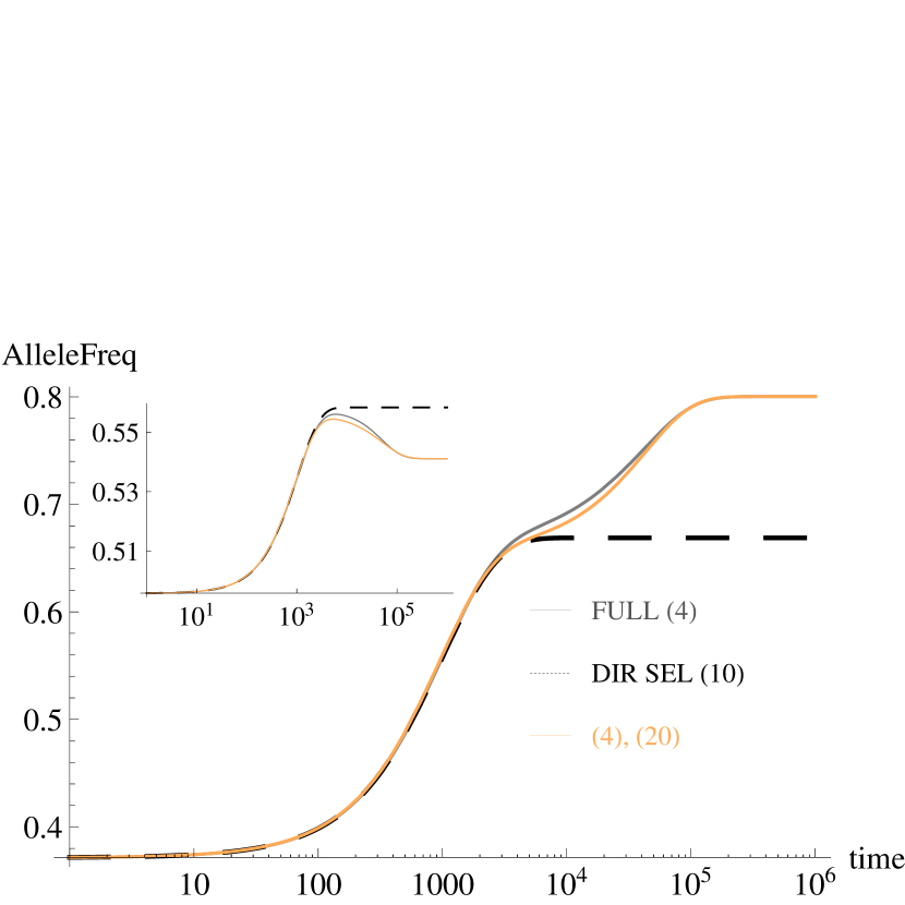
Figure 2: Most effects are small: Dynamics of the allele frequency for locus with effect $\gamma_{i}=0.121$ (main) and $\gamma_{i}=0.024$ (inset). All the parameters are the same as in Fig. 1. Note that while the initial allele frequency in the inset is closely approximated by (8), the allele trajectory starts at a value much lower than one half in the main panel as the effect size is close to ${\hat{\gamma}}\approx 0.126$. In the latter case, the corrections to (8) are substantial and given by (B2) of de Vladar and Barton (2014).

The correction to the equilibrium allele frequency in (8) when the stationary mean deviation is nonzero but small can be found in the Appendix B of de Vladar and Barton (2014). For future reference, we note that these corrections are negligible except when the effect is close to the threshold ${\hat{\gamma}}$ (see Fig. 2 below).

DYNAMICS WHEN MOST EFFECTS ARE SMALL

We now study the dynamics of the allele frequency when most effects are small (${\bar{\gamma}}\ll{\hat{\gamma}}$). Since the population is initially equilibrated to the phenotypic optimum at zero, the initial frequency at the $i$th locus is well approximated by (8) and close to one half when most effects are small. Then, as $p_{i}(t)\approx q_{i}(t)$ at short times, we can neglect the last two terms on the RHS of (6) compared to the first term to get (Jain and Stephan, 2015)

$${\dot{p}_{i}}=S_{i}p_{i}q_{i}~{},$$ (10)

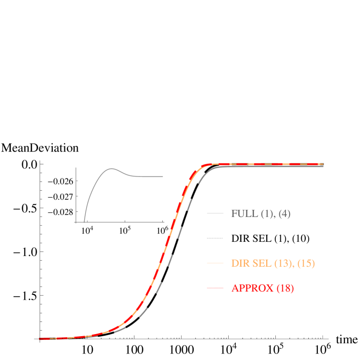
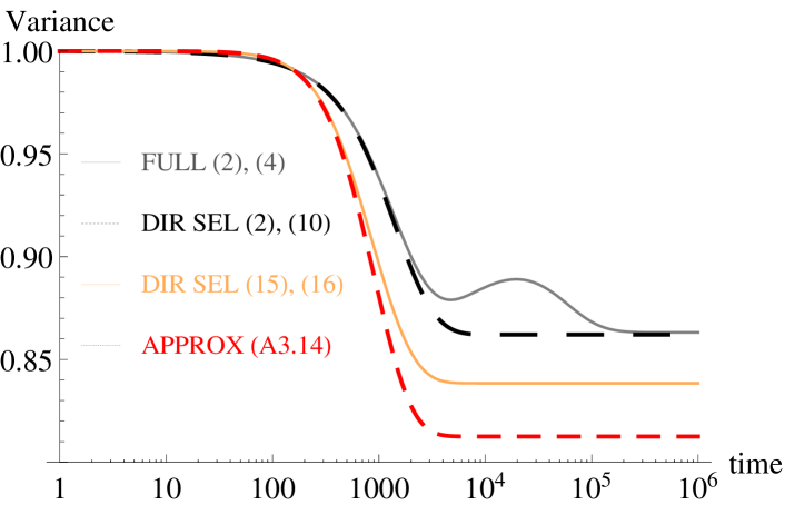
Figure 1: Most effects are small: Dynamics of the mean deviation and variance (relative to its initial value) for ${\hat{\gamma}}\approx 3.2{\bar{\gamma}}=0.128$ and $z_{f}=\ell{\bar{\gamma}}/4=2$. The other parameters are $s=5\times 10^{-3},\mu=10^{-5},{\bar{\gamma}}=0.04$. The inset in the top panel shows the mean deviation in the full model at large times. The gray and black curves are obtained for a single realization of effects in which $197$ out of $\ell=200$ loci have effects smaller than the mean. The orange and red curves, on the other hand, are averaged over the distribution of effects. The results from the two procedures match when the number of loci is very large as explained in DISCUSSION.

where $S_{i}=-s\gamma_{i}\Delta c_{1}$ and $\Delta c_{1}=c_{1}-z_{f}$. When the final mean deviation is negligible, the final allele frequency is also close to one half and we expect that (10) can describe the bulk of the allele frequency dynamics as is indeed supported by Figs. 1 and 2.

Directional selection model: In the following, we will refer to the model defined by (10) as the directional selection model. Appendix C details the prescription for calculating relevant quantities analytically in this model. As shown in Appendix C, the trait mean can be written as

$$c_{1}(t)=\sum_{i=1}^{\ell}\gamma_{i}-\sum_{i=1}^{\ell}\frac{2\gamma_{i}}{1+\frac{p_{i}(0)}{q_{i}(0)}~{}e^{\beta{\gamma_{i}}/{\bar{\gamma}}}}~{},$$ (11)

where the parameter $\beta$ defined in (C.6) is proportional to the logarithm of the ratio of allele frequencies and evolves in time as

$${\dot{\beta}}=-s{\bar{\gamma}}\Delta c_{1}.$$ (12)

Thus a closed equation for $\beta(t)$ can be obtained by eliminating the mean using (11) and on plugging the result for $\beta(t)$ back in (11), the mean can be found. Furthermore, it is shown in Appendix C that in the directional selection model, the $n$th cumulant of the effect evolves according to (Bürger, 1991)

$${\dot{c}}_{n}=-s\Delta c_{1}c_{n+1}~{},~{}n\geq 1~{},$$ (13)

which shows that the $n$th cumulant $c_{n},n\geq 2,$ can be found once $c_{n-1}$ is known. Thus to describe the short-time dynamics, we will focus on the key equations (11) and (12).

We now return to (11) for the mean $c_{1}$ and analyze it when the number of loci is large. When most effects are small (${\hat{\gamma}\gg\bar{\gamma}}$), as mentioned above, the initial allele frequency is one half. Furthermore, as explained in DISCUSSION, the sum over the contribution from individual loci in (11) amounts to averaging over the distribution of effects when the number of loci is large. For large $\ell$, on approximating the sum in (11) by an integral, we thus get

$$c_{1}(t)={\ell{\bar{\gamma}}-\frac{\ell}{\bar{\gamma}}\int_{0}^{\hat{\gamma}}d\gamma\frac{2\gamma e^{-\gamma/{\bar{\gamma}}}}{1+e^{\beta{\gamma}/{\bar{\gamma}}}}}~{}.$$ (14)

Writing $x=\gamma/{\bar{\gamma}}$ in the above integral, we get

$$c_{1}(t)=\ell{\bar{\gamma}}(1-2I_{s}(\beta))~{},$$ (15)

where

$$I_{s}(\beta)=\int_{0}^{{\hat{\gamma}}/{\bar{\gamma}}}dx~{}\frac{xe^{-x}}{1+e^{\beta x}}~{}.$$ (16)

Our main task is to find the time dependence of $\beta$ using (12) and (15) which is dealt with in Appendix D.

Qualitative patterns of the cumulant dynamics: Before turning to explicit expressions, we first make some general remarks on the behavior of the cumulants in the directional selection model. Since the variance is always nonnegative, it follows from (13) that the magnitude of mean deviation decreases with time. As we are considering the scenario where $\Delta c_{1}(0)<0$, the mean deviation $\Delta c_{1}(t)$ increases monotonically with time towards zero as shown in Fig. 1. Due to (12), this also means that $\beta(t)$ initially increases and then saturates to a constant.

Furthermore, due to (12) and (13), the variance can be written as

$$c_{2}=-2\ell{\bar{\gamma}}^{2}I_{s}^{\prime}(\beta)~{},$$ (17)

where prime denotes the derivative with respect to $\beta$. To arrive at the above expression, we have used that ${\dot{c}}_{1}=-2\ell{\bar{\gamma}}I_{s}^{\prime}(\beta){\dot{\beta}}$ due to (15). Equation (17) gives the rate of change of variance as ${\dot{c}}_{2}=-2\ell{\bar{\gamma}}^{2}{\dot{\beta}}~{}I_{s}^{\prime\prime}(\beta)$. It is easy to check that the integrand of $I_{s}^{\prime\prime}$ is always positive from which it follows that $I_{s}^{\prime\prime}(\beta)>0$. Therefore the directional selection model predicts that when most effects are small, the variance decreases with time as indeed verified in Fig. 1. From this result and (13), it immediately follows that the skewness $c_{3}$ defined in (A.6) is always negative.

Quantitative dynamics of the mean and higher cumulants: As shown in Appendix D, the mean deviation vanishes exponentially fast,

$$\Delta c_{1}(t)=\Delta c_{1}(0)e^{-sc_{2}(0)t}~{},$$ (18)

where $c_{2}(0)\approx\ell{\bar{\gamma}}^{2}$ is the initial variance given by (9) when most effects are small. The above result has been previously obtained by assuming that the variance and higher cumulants do not evolve in time (Lande, 1983; Chevin and Hospital, 2008; Jain and Stephan, 2015). The basis of this assumption lies in phenotypic data (Lande, 1976) or is motivated by mathematical tractability (Chevin and Hospital, 2008; Gomulkiewicz et al., 2010; Jain and Stephan, 2015). Here, in contrast, we have obtained (18) without any additional assumptions.

Using the solution (18) in (13) for cumulant dynamics, we find that the variance stays at its initial value $c_{2}(0)$ and the higher cumulants vanish. The corrections to these behavior at late times are given by (D.13) and (D.14), and we find that the variance remains a constant at short times ($\ll(sc_{2}(0))^{-1}$) but decreases thereafter to a smaller value:

$$\frac{c_{2}(t)}{c_{2}(0)}\approx 1-3\left(\frac{z_{f}}{\ell{\bar{\gamma}}}\right)^{2}(1-e^{-sc_{2}(0)t})^{2}~{}.$$ (19)

The above expression shows that the drop in the variance is larger for large shifts in the optimum and can be quite significant as shown in Fig. 1 for a moderate shift (relative to the maximum mean). A comparison between the full model, directional selection model and the analytical results is also shown in Fig. 1 for mean and variance. The reason for the difference observed in Fig. 1 between the cumulants obtained using (10) and the large-$\ell$ approximation (15) is explained in DISCUSSION.

The main panel of Fig. 1 shows that the mean is very close to the stationary state at time $t\approx 5000$. However, as shown in the inset, the mean continues to change albeit very slowly until $t\approx 2\times 10^{5}$ when the true stationary state is reached. A similar pattern is seen for variance (and allele frequency shown below in Fig. 2). These observations suggest that the dynamics of the mean can be divided into a short-term phase in which the mean approaches a value close to the new optimum and a long-term phase in which it reaches the exact stationary state. To explore fast evolution, we will concentrate in the following on the short-term phase.

Dynamics of the allele frequencies: From (10) for allele frequency dynamics, we first note that for $\Delta c_{1}(0)<0$, all the $+$ allele frequencies increase in the short-term phase (note that so far, we have argued that (10) holds for small-effect loci only but in the next section, we will find this to be true for large-effect loci also). This simple result has potentially useful application as explained in DISCUSSION.

Using (18) in (10), the time dependence of the allele frequency for small deviations in the phenotypic optimum can be obtained analytically (Chevin and Hospital, 2008; Jain and Stephan, 2015):

$$p_{i}(t)=\frac{p_{i}(0)}{p_{i}(0)+q_{i}(0)\exp\left(-\frac{z_{f}\gamma_{i}(1-e^{-s\ell{\bar{\gamma}}^{2}t})}{\ell{\bar{\gamma}}^{2}}\right)}~{}.$$ (20)

Thus in the directional selection model, the allele frequency reaches the stationary state over a time period $\sim(s\ell{\bar{\gamma}}^{2})^{-1}$. These shifts in allele frequency are small to moderate, as verbally predicted by several authors (e.g. Pritchard and Di Rienzo (2010)). However, this directional behavior may change in the long-term period, as we will discuss next.

The allele frequency dynamics in the full model and directional selection model are compared for some loci in Fig. 2, and we see that while the two match well at short times, in the full model, the allele frequency at large times can vary in a nonmonotonic fashion (see inset of Fig. 2) and approaches a stationary state value given by the solution of (7). The long-time dynamics of the allele frequency can be understood by solving (6) with zero mean deviation and the initial condition given by the stationary state solution of the directional selection model (Jain and Stephan, 2015). A succinct way of expressing such a prescription is to write

$$\Delta c_{1}(t)=\Delta c_{1}^{*}+\Delta c_{1}(0)e^{-sc_{2}(0)t}$$ (21)

in (6). Numerical integration of the resulting equation matches well with the full model as shown in Fig. 2. An analytical understanding of the long-time dynamics can also be obtained as described in Appendix E.

DYNAMICS WHEN MOST EFFECTS ARE LARGE

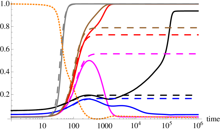
Figure 3: Selective sweeps when most effects are large: Dynamics of the scaled absolute mean deviation $|\Delta c_{1}(t)|/z_{f}$ (dotted, orange) and allele frequency (solid and dashed curves) for some loci that satisfy the necessary condition $\gamma_{i}<-2\Delta c_{1}(0)$ where $\Delta c_{1}(0)=-2.99$ and $z_{f}=3$. The numerical solution of the full model (6) (solid) and directional selection model (10) (dashed) are shown for the effect size $\gamma_{i=1,...,6}=0.776$ (gray), $0.340$ (brown), $0.319$ (red), $0.272$ (magenta), $0.092$ (blue), $0.060$ (black). The other parameters are $s=0.1,\mu=10^{-4},{\bar{\gamma}}=0.2,\ell=20$. Except for the locus with effect $\gamma_{4}$, the allele frequency for the directional selection model exceeds one half at loci whose allele frequency for the full model sweeps. The allele frequency for the locus with effect $\gamma_{6}$ also increases nearly to fixation but at very long times where the directional selection model is not valid. Because this frequency increase is relatively slow, a genomic signature similar to a selective sweep cannot be expected.

We now turn to the situation when most effects are large (${\bar{\gamma}}\gg{\hat{\gamma}}$). Due to (8), the initial allele frequencies are close to either zero or one. When the final mean deviation is close to zero, either the final allele frequency stays close to the initial one or sweeps to fixation as shown in Fig. 3. Thus, unlike in the case where most effects are small, in the full model the factor $q_{i}-p_{i}$ in the last two terms on the RHS of (6) is not negligible. However, the directional selection model defined by (10) describes the short-time dynamics when most effects are large as explained below.

Since we are dealing with the case where ${\hat{\gamma}}\ll\gamma_{i}$, we can ignore the effect of mutations. Furthermore, as $|q_{i}-p_{i}|$ can not exceed one, (6) shows that as long as $2|c_{1}(t)-z_{f}|\equiv 2|\Delta c_{1}(t)|\gg\gamma_{i}$, the second term on the RHS can be neglected to yield (10) for the allele frequency at the $i$th locus. Therefore we expect the directional selection model to apply at short times. But as time progresses, the mean deviation decreases in magnitude and the above condition for the validity of the directional selection model fails.

Using the initial frequency given by (8) for $\gamma_{i}\gg{\hat{\gamma}}$, equation (11) for the mean yields

$$c_{1}(t)=\sum_{i=1}^{\ell}\gamma_{i}-\sum_{i\in{P}^{+}}\frac{2\gamma_{i}}{1+\frac{p_{i}^{+}(0)}{q_{i}^{+}(0)}e^{{\beta\gamma_{i}}/{\bar{\gamma}}}}-\sum_{i\in P^{-}}\frac{2\gamma_{i}}{1+\frac{p_{i}^{-}(0)}{q_{i}^{-}(0)}e^{\beta{\gamma_{i}}/{\bar{\gamma}}}}~{},$$ (22)

where $P^{\pm}$ refers to the set of loci with initial frequencies $p_{i}^{\pm}(0)$ given in (8). From symmetry considerations, we expect the number of loci with initial frequency above and below one half to be equal. Furthermore, for $\gamma_{i}\gg{\hat{\gamma}}$, the initial allele frequency given by (8) can be approximated as $p_{i}^{-}(0)\approx(\frac{{\hat{\gamma}}}{2\gamma_{i}})^{2},p_{i}^{+}(0)=1-p_{i}^{-}(0)$. We thus arrive at

$$c_{1}(t)\approx\sum_{i=1}^{\ell}\gamma_{i}-\sum_{i\in{P}^{+}}\frac{2\gamma_{i}}{1+\left(\frac{2\gamma_{i}}{\hat{\gamma}}\right)^{2}e^{{\beta\gamma_{i}}/{\bar{\gamma}}}}-\sum_{i\in P^{-}}\frac{2\gamma_{i}}{1+\left(\frac{\hat{\gamma}}{2\gamma_{i}}\right)^{2}e^{\beta{\gamma_{i}}/{\bar{\gamma}}}}~{}.$$ (23)

Then, as in the last section, approximating the sums in (23) by integrals for large $\ell$, we get

$${c_{1}(t)}={\ell{\bar{\gamma}}}(1-I_{l}^{+}-I_{l}^{-})~{},$$ (24)

where

$$I_{l}^{+} = {\color[rgb]{0,0,0}\frac{1}{2\bar{\gamma}}\int_{\hat{\gamma}}^{\infty}d\gamma\frac{2\gamma e^{-\gamma/{\bar{\gamma}}}}{1+\left(\frac{2\gamma}{\hat{\gamma}}\right)^{2}e^{{\beta\gamma}/{\bar{\gamma}}}}}$$ (25)

$$= \int_{2/\alpha}^{\infty}dx~{}\frac{xe^{-x}}{1+(\alpha x)^{2}e^{\beta x}}~{},$$ (26)

and

$$I_{l}^{-} = {\color[rgb]{0,0,0}\frac{1}{2\bar{\gamma}}\int_{\hat{\gamma}}^{\infty}d\gamma\frac{2\gamma e^{-\gamma/{\bar{\gamma}}}}{1+\left(\frac{\hat{\gamma}}{2\gamma}\right)^{2}e^{{\beta\gamma}/{\bar{\gamma}}}}}$$ (27)

$$= \int_{2/\alpha}^{\infty}dx~{}\frac{xe^{-x}}{1+(\alpha x)^{-2}e^{\beta x}}~{}.$$ (28)

In the above equations, the parameter $\alpha=2{\bar{\gamma}}/{\hat{\gamma}}$.

Qualitative patterns: In the directional selection model, as (12) and (13) hold irrespective of whether most effects are small or large, the mean deviation $\Delta c_{1}(t)$ and the allele-frequency-dependent variable $\beta$ increase with time as discussed in the last section, and the variance is given by $c_{2}=-\ell{\bar{\gamma}}^{2}(I_{l}^{+^{\prime}}+I_{l}^{-^{\prime}})$. However, unlike when most effects are small, here the rate of change of variance, ${\dot{c}}_{2}=s{\ell}{\bar{\gamma}}^{3}\Delta c_{1}(I_{l}^{+^{\prime\prime}}+I_{l}^{-^{\prime\prime}})$ is not a monotonic function of time; this is because the sum $I_{l}^{+^{\prime\prime}}+I_{l}^{-^{\prime\prime}}$ is negative when $\beta$ is small and positive for larger $\beta$. Thus the directional selection model predicts that initially the variance increases with time and then decreases towards the stationary state at the new phenotypic optimum.

Quantitative dynamics: Equation (24) along with (12) forms a closed system of equations and allows us to find the mean. The integrals $I_{l}^{\pm}$ are estimated in Appendix F; we find that the integral $I_{l}^{+}$ does not contribute substantially to the mean since it includes the loci with initial frequency close to one and we are dealing with the case when the initial mean deviation is negative (see also (32) below), and $I_{l}^{-}$ is well approximated by $J_{l}$ given by (F.8). When the initial deviation from the phenotypic optimum is small, using (F.14) and (F.21), we find that at large times, the mean deviation decreases exponentially fast,

$$\Delta c_{1}(t) \sim e^{-s\ell{\bar{\gamma}}^{2}(\ln\alpha)^{-1}\rho(\ln\rho)^{2}t}~{},$$ (29)

$$= e^{-sz_{f}{\bar{\gamma}}(\ln\alpha)^{-1}(\ln\rho)^{2}t}~{},$$ (30)

where $\rho=z_{f}/(\ell{\bar{\gamma}})$ is the phenotypic shift relative to the maximum mean magnitude. The above result shows that time scale over which the mean approaches the stationary state depends weakly on the number of loci unlike the case when most effects are small (see (18)). However as the mean of the distribution is large here, the relaxation in the directional selection model occurs faster than in the small-effects case.

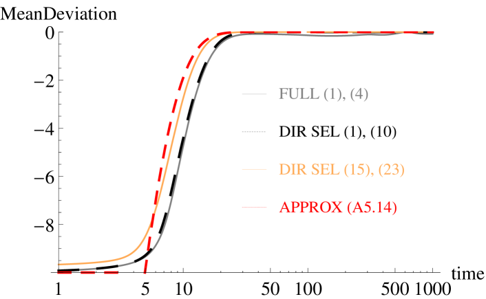
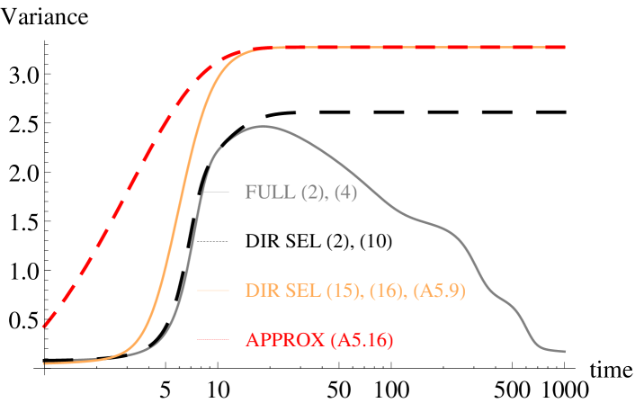
Figure 4: Most effects are large: Dynamics of the mean deviation for ${\hat{\gamma}}\approx 0.028,{\bar{\gamma}}=10{\hat{\gamma}}$ and $z_{f}=10\approx 0.18\ell{\bar{\gamma}}$. For the realization of effects used in this figure, $183$ out of $\ell=200$ loci have effects larger than the mean. The other parameters are $s=0.1,\mu=10^{-5}$ .

When most effects are large, the variance changes considerably even when the relative phenotypic shift is quite small as Fig. 4 shows. The peak variance $c_{2}^{(\textrm{max})}$ can be estimated by the stationary state variance in the directional selection model. At large times, using (F.16) and (F.21), we find that

$$c_{2}^{(\textrm{max})}=\ell{\bar{\gamma}}^{2}(\ln\alpha)^{-1}\rho(\ln\rho)^{2}$$ (31)

and therefore $c_{2}^{(\textrm{max})}/c_{2}(0)\sim\alpha^{2}\gg 1$. This result can also be seen by noting that the allele frequencies at loci with initial frequency close to zero shift to intermediate values at short times. Then from (4), the maximum variance is obtained when the allele frequency is close to one half leading to $c_{2}^{(\textrm{max})}\sim\ell{\bar{\gamma}}^{2}$.

The dynamics of the allele frequency at long times are discussed in Appendix E and at short times in the next section.

WHEN DO SELECTIVE SWEEPS OCCUR?

Below we obtain a criterion on the size of effects for which the allele frequency at a major locus can sweep. When $p_{i}(0)\approx 0$, at short enough times, keeping only the lowest order terms in $p_{i}$ on the RHS of the full model (6) and neglecting the effect of mutations, we get

$${\dot{p}}_{i}\approx-\frac{s\gamma_{i}p_{i}}{2}(2\Delta c_{1}(0)+\gamma_{i})~{}.$$ (32)

When the initial mean deviation $\Delta c_{1}(0)<0$, the above equation shows that only the loci with effect $\gamma_{i}<2|\Delta c_{1}(0)|$ can potentially sweep since their frequency increases with time. On repeating the above analysis for loci with initial frequency close to one, we find that the frequency at such loci does not sweep to zero. Thus, when $\Delta c_{1}(0)<0$, only the loci with small initial frequency and effect $<2|\Delta c_{1}(0)|$ are likely to undergo large changes in the frequency. These criteria are necessary but as Fig. 3 shows, they are not sufficient for a selective sweep to occur.

For the major loci that meet the above necessary conditions for selective sweeps, the second and the third term on the RHS of the full model (6) can be neglected in comparison to the first term thereby reducing (6) to the directional selection model (10). For the rest of the (major) loci, the allele frequency changes are not appreciable and the frequencies remain close to zero or one, a solution satisfied by (10). Let ${\tilde{t}}$ denote the time when the allele frequencies evolving according to the directional selection model equilibrate. Figure 3 shows that the mean deviation obtained using the full model is close to zero at time ${\tilde{t}}$. Then for subsequent times $t>{\tilde{t}}$, we can ignore mutations and set $\Delta c_{1}=0$ in the full model (6) to obtain (Jain and Stephan, 2015)

$${\dot{p}}_{i}=\frac{s\gamma_{i}^{2}}{2}p_{i}q_{i}(2p_{i}-1)~{},~{}t>{\tilde{t}}~{}.$$ (33)

The above differential equation is subject to the initial condition $p_{i}({\tilde{t}})$ which is the allele frequency in the steady state of the directional selection model.

From the definition (C.6) of $\beta$, we have

$$\frac{p_{i}({\tilde{t}})}{1-p_{i}({\tilde{t}})}=\frac{p_{i}(0)}{q_{i}(0)}\exp\left(\frac{\gamma_{i}{\tilde{\beta}}}{\bar{\gamma}}\right)$$ (34)

which simplifies to give the frequency $p_{i}({\tilde{t}})$ as

$$p_{i}({\tilde{t}})=\left[1+\frac{q_{i}(0)}{p_{i}(0)}\exp\left(-\frac{\gamma_{i}{\tilde{\beta}}}{\bar{\gamma}}\right)\right]^{-1}~{},$$ (35)

where ${\tilde{\beta}}\equiv\beta(\tilde{t})$. It is clear from (33) that if the frequency $p_{i}({\tilde{t}})$ is greater than one half, the allele frequency at the $i$th locus will increase monotonically towards one. Thus we predict that the allele frequency at a locus would sweep when $p_{i}({\tilde{t}})>1/2$. Combining this criterion with the necessary condition mentioned above, we find that a sweep can occur when the effects lie in the following range:

$$\frac{\bar{\gamma}}{\tilde{\beta}}\ln\left(\frac{q^{-}_{i}(0)}{p^{-}_{i}(0)}\right)<\gamma_{i}<2z_{f}.$$ (36)

This expectation is indeed seen to be consistent with the numerical solution of the full model as shown in Fig. 3 except for one case.

When most effects are small: While considering the dynamics of mean and variance when most effects are small in an earlier section, we ignored the contribution of (few) loci that have large effect. However the results obtained earlier can be utilized to understand the dynamics of the allele frequency at major loci also. As (D.11) shows, the auxiliary parameter in the stationary state of the directional selection model is ${\tilde{\beta}}=z_{f}/(\ell{\bar{\gamma}})$. Using this in (36), we find that a selective sweep can occur at a major locus if its effect

$$2z_{f}>\gamma_{i} > \frac{\ell\bar{\gamma}^{2}}{z_{f}}\ln\left(\frac{q^{-}_{i}(0)}{p^{-}_{i}(0)}\right)~{},~{}$$ (37)

$$= \frac{c_{2}(0)}{|\Delta c_{1}(0)|}\ln\left(\frac{q^{-}_{i}(0)}{p^{-}_{i}(0)}\right)~{},$$ (38)

which matches the criterion (26b) of Chevin and Hospital (2008). Furthermore, using (8), we find that

$$\frac{2c_{2}(0)}{|\Delta c_{1}(0)|}\ln\left(\frac{2\gamma_{i}}{{\hat{\gamma}}}\right)<\gamma_{i}<2z_{f}~{}.$$ (39)

For the parameters in Fig. 1 where the average effect size ${\bar{\gamma}}=0.04$ and the threshold effect ${\hat{\gamma}}=0.128$, the above criterion requires that the effect size at a major locus be $>0.81$. For exponentially distributed effects, as is assumed in this article, the probability for the effect size to exceed this criterion is extremely low ($\sim 10^{-9}$ for the parameters in Fig. 1) and therefore selective sweeps at major loci are prevented when most effects are small (Chevin and Hospital, 2008; Pavlidis et al., 2012).

When most effects are large: The criterion for short-time sweeps is more involved in this case; using (8) in (36), we obtain

$$2z_{f}>\gamma_{i} > \frac{2\bar{\gamma}}{\tilde{\beta}}\ln\left(\frac{2\gamma_{i}}{{\hat{\gamma}}}\right)~{},~{}$$ (40)

$$\approx \frac{2\bar{\gamma}}{\ln\left(\frac{2{\bar{\gamma}}}{\hat{\gamma}}\right)}\ln\left(\frac{\ell{\bar{\gamma}}}{z_{f}}\right)\ln\left(\frac{2\gamma_{i}}{{\hat{\gamma}}}\right)~{},$$ (41)

where we have used (F.20) for $\tilde{\beta}$ in the last expression. For the parameters in Fig. 4, using ${\tilde{\beta}\approx 2.32}$ in (40), we find that for a selective sweep to occur, $\gamma_{i}>1.04$ is required whose probability is $\approx 0.024$. In other words, we expect as many as $0.024\times 200\approx 5$ sweeps to occur for these parameter values over the time scale the mean deviation approaches zero.

DISCUSSION

Dynamical regimes in the full model: Figure 3 shows an example of the dynamics of the mean and allele frequencies when an infinitely large population in linkage equilibrium and equilibrated to a phenotypic optimum is suddenly shifted to a new optimum. We observe a short-term phase $(t\lesssim 10^{3})$ where the mean deviation increases quickly to a value close to zero followed by a long-term phase $(10^{3}<t<10^{5})$ where the mean deviation undergoes minor changes at a slow pace. The former phase where the adaptation process is rapid is the focus of this article since: (i) much of the action happens in this early phase (for example, in Fig. 3, the allele frequencies at $13$ out of $20$ loci were close to the stationary state at the end of the short-term phase), (ii) these time scales are experimentally observable, and very importantly, (iii) all $+$ alleles increase in frequency in a synergistic manner.

Directional selection model: Although the full model defined by (6) can be investigated numerically (de Vladar and Barton, 2014), as the allele frequency dynamics at a single locus are related to all the other $\ell-1$ loci via the phenotypic mean (first term on the RHS of (6)), it is difficult to obtain analytical results. Moreover, the full model results in equations for the cumulants that do not close, and therefore one resorts to an often unjustified and uncontrolled approximation of setting all the cumulants above a certain number to zero (see Barton and de Vladar (2009) for a discussion of this approach). This approximation, however, works quite well when most effects are small (Jain and Stephan, 2015) but fails completely when most effects are large (see supplemental file S1 for a detailed explanation).

Here we have devised an approximate model (directional selection model) defined by (10) in which the allele frequencies are coupled but nonetheless, one can make analytical progress without truncating the cumulants arbitrarily. The central equations in the directional selection model are (11) and (12) that relate the mean deviation and an auxiliary parameter $\beta$ which is a function of a single allele frequency. As explained in Appendices D and F, it is possible to obtain explicit expressions for the time dependence of $\beta$ and thereby that of the mean. Higher cumulants such as the variance can be then found using (13).

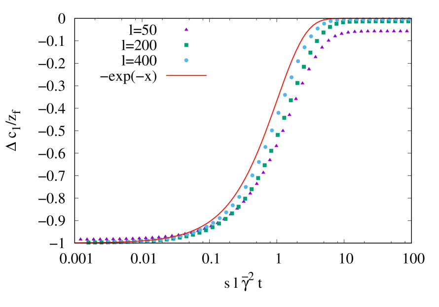
Figure S1: Mean deviation for various values of the number of loci and fixed $z_{f}={\ell{\bar{\gamma}}}/4$ for the parameters in Fig. 1 to show that the numerical data obtained in the full model (6) for a single set of effects approaches the analytical expression (18) with increasing $\ell$.

Distribution of effects: All the numerical examples shown in the figures use a single realization of the effect at a locus, i.e., one set of effects $\{\gamma_{i}\}~{},~{}i=1,...,{\ell},$ are chosen from an exponential distribution. For additive quantities such as mean and variance that are obtained by summing the contribution over a number of loci, we expect that a single realization of effects is a good representative when the number of loci are sufficiently large (in physics literature, this concept is known as self-averaging (Castellani and Cavagna, 2005)). A similar idea has been used recently in a model of stabilizing selection with the same effects at all loci in which the phenotypic mean for one set of initial allele frequencies is approximated by the corresponding average (Charlesworth, 2013). Figure S1 shows that the quantitative agreement between the results for the mean deviation obtained for a single realization of phenotypic effects for $\ell=50,200,400$ and the analytical result for large $\ell$ gets better as the number of loci increase.

Main results: The key conclusions of this article are discussed below and summarised in Table 1.

	Mean dynamics	Variance dynamics	Selective sweeps
	determined by	characterised by	at major loci
Small effects	Initial variance (18)	Small variations (19)	Unlikely (39)
Large effects	Effect size (30)	Large variations (31)	Probable (41)

Table 1: Summary of the results for the dynamics of phenotypic mean, variance and allele frequency when the phenotypic optimum is suddenly shifted.

Response of the mean to a sudden shift of the phenotypic optimum: How does the time scale over which the mean reaches the stationary state depend on various factors such as the number of loci, initial phenotypic mean deviation and size of the effects? We find that the mean deviation becomes negligible on a time scale that is inversely proportional to the number of loci ($\ell$) when most effects are small but depends weakly on $\ell$ when most effects are large (cf. (18) and (30)). This difference in the behavior may be understood as follows: when most effects are small, there is sufficient genetic variation initially for selection to act on because a large number of loci are initially polymorphic. Therefore, with increasing $\ell$, the equilibration time decreases. In contrast, when most effects are large, the initial genetic variation is negligible and the adaptation dynamics are determined by the size of the effects. As the availability of large-effect loci depends on the mean of the effect distribution, it follows that the larger the mean, the faster the adaptation dynamics.

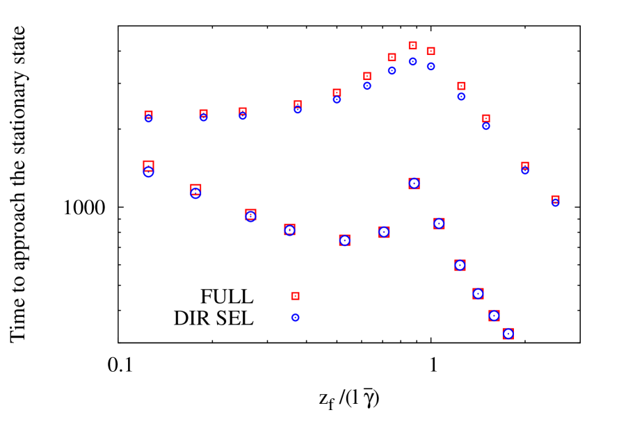
Figure 5: Small vs. large effects when the number of loci are same: Time at which the mean reaches $0.9$ of the exact stationary state mean $c_{1}^{*}$ for various values of $z_{f}$ when most effects are small (small symbols) and large (large symbols). For the former (latter) case, the rest of the parameters are the same as in Fig. 1 (4). In order to show the data in the two cases on the same scale, the time for the large-effect case has been multiplied by $70$.

Figure 5 shows that the relationship between the equilibration time and the initial mean deviation depends on the size of effects (see also Gomulkiewicz et al. (2010)). When most effects are large, selective sweeps occur at some loci that result in drastic changes in the allele frequencies thus accelerating the approach to the phenotypic optimum. But when most effects are small, the equilibration time remains roughly constant as selective sweeps do not occur but small changes in the allele frequencies at a large number of loci drive the adaptation process. Figure 5 also shows that when the number of loci contributing to a trait are the same, adaptation is faster when the effect size is larger, which makes intuitive sense.

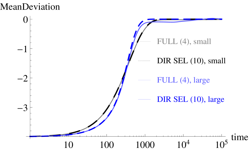
Figure 6: Many loci with small effects vs. few loci with large effects: Mean deviation as a function of time when most effects are small (${\bar{\gamma}}=0.04,\ell=400$) and large (${\bar{\gamma}}=0.32,\ell=50$). In both cases, ${\hat{\gamma}}\approx 0.126$ ($s=5\times 10^{-3},\mu=10^{-5}$) and the new phenotypic optimum is shifted to $z_{f}={\ell{\bar{\gamma}}}/4=4$.

However one may also compare situations in which a large number of small effects control a phenotypic trait with the one in which few loci with large effects contribute to a trait. An example shown in Fig. 6 suggests that the adaptation at short times is faster when effects are small but at longer times, larger effects lead to rapid adaptation. This conclusion is borne out by our analysis as well: on comparing (18) and (30), we find that for identical $z_{f}$ and $\ell{\bar{\gamma}}$, the time scales are inversely proportional to $\bar{\gamma}$ and therefore it takes shorter time to equilibrate in the large-effect case.

An important omission in the above discussion is random genetic drift as we have considered infinitely large populations. Some progress in this regard has been made recently (Matuszewski et al., 2015; Bod’ová et al., 2016); however, a detailed analysis is currently not available and would be interesting to consider in the future.

Dynamics of the variance and allele frequencies: Besides the dynamics of the mean, we also studied the time dependence of the variance. We find that at short times, the variance does not vary much and decreases monotonically with time when most effects are small. This behavior can be explained by the fact that the allele frequencies show small to moderate changes. In the opposite case, the variance changes considerably and its variation is nonmonotonic in time - it increases at short times and then decreases to the stationary state value. The selective sweeps at major loci are responsible for this effect. The rate of change of average fitness given by (C.9) receives contributions from the square of the mean deviation and the rate of change of variance. Thus when most effects are large, at short times, the average fitness increases more slowly in the short-term phase than at longer times (Gomulkiewicz et al., 2010).

The directional selection model describes the bulk of the mean dynamics in the short-term phase. Therefore at late times where the mean deviation is close to zero, the allele frequency at each locus evolves independently (the first term on the RHS of (6) is zero) and the dynamics are much slower as described in Appendix E. At short times, the allele frequency dynamics involve the same time scales as for the mean and variance.

Applications: The analysis of our model relates to various important questions that are currently discussed in evolutionary genetics.

Rapid adaptation: The approximations we have presented here describe the short-term evolution of a phenotypic trait after a sudden environmental change very well. We have shown that the mean of a phenotypic trait may respond very fast after an environmental shift. In the case that most effects are small, this is possible because the time to the new optimum is inversely proportional to the number of loci controlling the trait. In the opposite case of mostly large effects, rapid fixations (leading to selective sweeps) may produce fast phenotypic responses. In the examples of fast adaptation mentioned in INTRODUCTION both of these extremes and combinations thereof have occurred.

QTL and selective sweep mapping: Selective sweep mapping has been used to dissect QTL (Svetec et al., 2011; Rubin et al., 2012; Axelsson et al., 2013; Wilches et al., 2014). However, the success of this approach was varied. Nonetheless, there seems to be a tendency that it worked better in domesticated than in natural populations (Rubin et al., 2012; Axelsson et al., 2013), probably due to the action of artificial selection during domestication. In artificial selection, the shift to the new optimum $z_{f}$ may be larger than under natural conditions; our criterion (36) thus indicates an enhancement of sweeps in domesticated populations.

More generally, our analysis provides also some new insights into the question whether selective fixations (and thus sweeps) occur at QTL. While Chevin and Hospital (2008) predicted that the probability of selective sweeps is extremely low at QTL (based on a model with one major locus and infinitely many minor loci), others have found sweeps at appreciable frequencies using simulations of various multi-locus models (Pavlidis et al., 2012; Wollstein and Stephan, 2014). The prediction of Chevin and Hospital is consistent with our study for mostly small-effect loci and small shifts in the phenotypic optimum.

Testing for fast polygenic adaptation: Using standardized frequencies, one can construct tests to detect SNPs that deviate strongly from neutral population structure (e.g. Coop et al. (2010)). However, this approach is only working if there exist relatively large extended gradients of ecological variables, which may not be the case in rapid adaptation. Shortly after a population occupies a new habitat, we expect that the allele frequency shifts between the parental and derived populations are relatively small. This also means that available software, such as BayeScan-like methods (Foll and Gaggiotti, 2008; Riebler et al., 2008), is not able to detect significant frequency shifts for individual SNPs between populations. Therefore, for detecting small allele frequency shifts after environmental changes in fast adapting populations, it may be best to consider the frequency shifts of alleles simultaneously at all loci involved (instead of individual SNPs). Our results suggest that this may be a promising approach, as all + alleles shift their frequencies in the same direction in the short-term phase, which should increase the power of the test. In human population genetics, this approach has been used to analyze recent polygenic adaptation for instance of height (Turchin et al., 2012).

Acknowledgements: We thank the ICTS, Bangalore, for their hospitality during the Second Bangalore School on Population Genetics and Evolution (ICTS/Prog-popgen/2016/01) that facilitated our discussions. Furthermore, we are grateful to Graham Coop and two anonymous reviewers who made valuable suggestions to improve the paper. The research of WS was supported by the German Research Foundation DFG (grant Ste 325/17-1 from the Priority Program 1819).

APPENDIX

Appendix A Cumulants of the effects and their dynamics

The effect $e_{i}$ at the locus $i$ is distributed according to a Bernoulli distribution

$$p(e_{i})=p_{i}\delta_{e_{i},\frac{\gamma_{i}}{2}}+q_{i}\delta_{e_{i},-\frac{\gamma_{i}}{2}}~{}.$$ (A.1)

The generating function of the distribution of the effects at the $i$th locus is given by

$$F_{i}(\xi)=\sum_{e_{i}}p(e_{i})e^{-e_{i}\xi}=p_{i}e^{-\frac{\gamma_{i}}{2}\xi}+q_{i}e^{\frac{\gamma_{i}}{2}\xi}~{}.$$ (A.2)

The logarithm of the generating function defines the $n$th cumulant $c_{n}^{(i)}$ at locus $i$ as (Sornette, 2000)

$$\ln F_{i}(\xi)=\sum_{n=1}^{\infty}c_{n}^{(i)}\frac{(-\xi)^{n}}{n!}=\frac{\xi\gamma_{i}}{2}+\ln\left(q_{i}+p_{i}e^{-\gamma_{i}\xi}\right)~{}.$$ (A.3)

The $n$th cumulant is then obtained as

$$c_{n}^{(i)}=(-1)^{n}\frac{d^{n}\ln F_{i}(\xi)}{d\xi^{n}}\Big{|}_{\xi=0}~{}.$$ (A.4)

In linkage equilibrium, since the cumulants for the $n$-locus problem are additive, we get

$$c_{n}=2\sum_{i=1}^{\ell}c_{n}^{(i)}~{},$$ (A.5)

where the factor of $2$ on the RHS takes care of diploidy. Using the last three equations above, we find that the mean and variance are given by (1) and (4), respectively. The skewness $c_{3}$ which is a measure of asymmetry of a distribution can also be found and given by

$$c_{3}=2\sum_{i=1}^{\ell}\gamma_{i}^{3}(q_{i}-p_{i})p_{i}q_{i}~{}.$$ (A.6)

Appendix B Quasi-linkage equilibrium approximation

For the additive genotype-phenotype map, the trait $z=\sum_{i=1}^{\ell}\gamma_{i}(X_{i}+X^{*}_{i}-1)$ where $X_{i},X^{*}_{i}=1(0)$ if the $+(-)$ allele is present at the locus $i$. Following Barton and Turelli (1991), we first find the association coefficients by writing $X_{i}=\langle X_{i}\rangle+\delta_{i},X^{*}_{i}=\langle X^{*}_{i}\rangle+\delta^{*}_{i}$ where $\langle X_{i}\rangle=\langle X^{*}_{i}\rangle=p_{i}$ and expanding the relative fitness to lowest orders in $s$,

$$\frac{w(\{X,X^{*}\})}{\overline{w}} = \frac{1-(s/2)(z-z^{\prime})^{2}}{{\overline{w}}}$$

$$\approx 1+\sum_{i=1}^{\ell}a_{i,\phi}(\delta_{i}-\langle\delta_{i}\rangle)+\sum_{i=1}^{\ell}a_{ii,\phi}(\delta_{i}^{2}-\langle\delta_{i}^{2}\rangle)$$

$$+ \sum_{i=1}^{\ell}a^{*}_{i,\phi}(\delta_{i}^{*}-\langle\delta_{i}^{*}\rangle)+\sum_{i=1}^{\ell}a^{*}_{ii,\phi}(\delta_{i}^{*2}-\langle\delta_{i}^{*2}\rangle)$$

$$+ \sum_{i<j}a_{ij,\phi}(\delta_{i}\delta_{j}-\langle\delta_{i}\delta_{j}\rangle)+\sum_{i<j}a^{*}_{ij,\phi}(\delta_{i}^{*}\delta_{j}^{*}-\langle\delta_{i}^{*}\delta_{j}^{*}\rangle)$$

$$+ \sum_{i,j=1}^{\ell}a_{i,j}(\delta_{i}\delta_{j}^{*}-\langle\delta_{i}\delta_{j}^{*}\rangle)~{}.$$ (B.2)

In the above equation, the average is taken with respect to the joint distribution of the frequencies at all the loci and the coefficients

$$a_{i,\phi}=-s(c_{1}-z^{\prime})\gamma_{i},~{}a_{ii,\phi}=-(s/2)\gamma_{i}^{2},~{}a_{ij,\phi}=a_{i,j}=-s\gamma_{i}\gamma_{j}~{}.$$ (B.3)

The average allele frequency change after selection (and recombination) is given by (see (10a), Barton and Turelli (1991))

$$\dot{p}_{i}=a_{i,\phi}\langle\delta_{i}^{2}\rangle+a_{ii,\phi}\langle\delta_{i}^{3}\rangle+\sum_{j\neq i}a_{j,\phi}\langle\delta_{i}\delta_{j}\rangle+\sum_{j\neq i}a_{jj,\phi}\langle\delta_{i}\delta_{j}^{2}\rangle+\sum_{j\neq k}a_{kj,\phi}\langle\delta_{i}\delta_{j}\delta_{k}\rangle~{}.$$ (B.4)

All but the first two terms on the RHS vanish in linkage equilibrium (LE); here we focus on the lowest order corrections to LE which are contained in the third and fourth terms. Using $X_{i}^{2}=X_{i}$ and $\langle\delta_{i}\rangle=0$, it is easy to show that $\langle\delta_{i}^{2}\rangle=p_{i}q_{i},\langle\delta_{i}\delta_{j}^{2}\rangle=(1-2p_{j})\langle\delta_{i}\delta_{j}\rangle$. Inserting these expressions in (B.4), we verify that the first two terms on the RHS match the corresponding ones in (6). The two-locus linkage disequilibrium evolves according to (see (12), Barton and Turelli (1991))

$$\dot{\langle\delta_{i}\delta_{j}\rangle}=-r_{ij}\langle\delta_{i}\delta_{j}\rangle+2a_{ij,\phi}\langle\delta_{i}^{2}\rangle\langle\delta_{j}^{2}\rangle+\textrm{higher order terms}~{},i\neq j~{},$$ (B.5)

where $r_{ij}$ denotes the recombination rate between the loci $i$ and $j$ and we have dropped terms that are nonlinear in the parameters $s$ and $r$ on the RHS of the above equation. Then at quasi-linkage equilibrium (QLE) where the LHS is of ${\cal O}(s^{2})$ or higher, we have

$$\langle\delta_{i}\delta_{j}\rangle_{QLE} \approx \frac{2a_{ij,\phi}}{r_{ij}}\langle\delta_{i}^{2}\rangle_{\textrm{LE}}\langle\delta_{j}^{2}\rangle_{\textrm{LE}}$$ (B.6)

$$= -\frac{2s\gamma_{i}\gamma_{j}}{r_{ij}}(p_{i}q_{i}p_{j}q_{j})|_{\textrm{LE}}~{},$$ (B.7)

where the allele frequencies in the last equation are in LE.

Using the above result in (B.4) and assuming that all the recombination rates are equal to $r$, we find that within QLE, the allele frequency obeys the following equation:

$$\dot{p}_{i}\approx-s\gamma_{i}p_{i}q_{i}(c_{1}-z^{\prime})\left(1-\frac{s}{r}c_{2,\textrm{LE}}\right)-\frac{s\gamma_{i}^{2}}{2}p_{i}q_{i}(q_{i}-p_{i})\left(1-\frac{s}{r}\frac{c_{3,\textrm{LE}}}{\gamma_{i}}\right)$$ (B.8)

where $c_{2,\textrm{LE}}$ and $c_{3,\textrm{LE}}$ are the variance and skewness, respectively, in linkage equilibrium. Thus, as expected, the corrections to the model defined by (6) are of order $s/r$ which can be neglected when selection and linkage are weak.

Appendix C Directional selection model

The dynamics of the allele frequency $p_{i}$ are described by (10) where the effective selection coefficient $S_{i}=-s\gamma_{i}\Delta c_{1}$ depends on all the allele frequencies through the mean $c_{1}$. This property makes it difficult to solve for the allele frequencies; however, we note that for two arbitrary loci $i$ and $m$, (10) gives

$$\frac{\dot{p}_{i}}{\dot{p}_{m}}=\frac{dp_{i}}{dp_{m}}=\frac{S_{i}p_{i}q_{i}}{S_{m}p_{m}q_{m}}~{},$$ (C.1)

which, on using the identity $d\left[\ln(p/q)\right]=dp/(pq)$, simplifies to

$$\frac{d\ln\varrho_{i}}{d\ln\varrho_{m}}=\frac{\gamma_{i}}{\gamma_{m}}~{},~{}i\neq m~{},$$ (C.2)

where $\varrho_{i}(t)={p_{i}(t)}/{q_{i}(t)}$. As the above equation does not involve the phenotypic mean, it can be easily solved to give

$$\varrho_{i}(t)=\varrho_{i}(0)\left(\frac{\varrho_{m}(t)}{\varrho_{m}(0)}\right)^{\frac{\gamma_{i}}{\gamma_{m}}}~{}.$$ (C.3)

We remark that the simple idea used in (C.1) to eliminate the global variable $\Delta c_{1}$ is quite similar to that employed in single-locus directional selection models to get rid of the average fitness (see, for example, p. 73, Charlesworth and Charlesworth (2010)).

Equation (C.3) is useful since it allows us to express the mean $c_{1}(t)$ in terms of a single allele frequency, say, at locus $m$. Using (C.3) in (1), we can write the mean as

$$c_{1}(t) = \sum_{i=1}^{\ell}\gamma_{i}\left(\frac{\varrho_{i}-1}{\varrho_{i}+1}\right)$$ (C.4)

$$= \sum_{i=1}^{\ell}\gamma_{i}-\sum_{i=1}^{\ell}\frac{2\gamma_{i}}{1+\varrho_{i}(0)\left(\frac{\varrho_{m}(t)}{\varrho_{m}(0)}\right)^{\frac{\gamma_{i}}{\gamma_{m}}}}~{},$$ (C.5)

which simplifies to give (11). In the above equation,

$${\beta(t)}=\frac{\bar{\gamma}}{\gamma_{m}}\ln\left(\frac{\varrho_{m}(t)}{\varrho_{m}(0)}\right)=\frac{\bar{\gamma}}{\gamma_{m}}\ln\left(\frac{p_{m}(t)}{p_{m}(0)}\frac{q_{m}(0)}{q_{m}(t)}\right)~{}.$$ (C.6)

Note that in the expression (C.5), although the dynamics of the mean deviation are determined by that of the allele frequency $p_{m}$, the rest of the $\ell-1$ frequencies are not redundant as the mean depends on their initial state also.

Furthermore, from the evolution equation (10) for the allele frequency, we also have ${\dot{\beta}}=-s{\bar{\gamma}}\Delta c_{1}$, where the mean is given by (C.5); we have thus obtained a closed equation for $\beta(t)$. Using the result for $\beta(t)$ in (C.5), the dynamics of the phenotypic mean can be calculated. This knowledge then allows us to find higher cumulants using (13) which is derived below.

To obtain the evolution equation (13) for the $n$th cumulant, we take the derivative with respect to time in (A.3) and use (10) for the allele frequency dynamics to obtain (Bürger, 1991)

$$\sum_{n=1}^{\infty}{\dot{c}}_{n}^{(i)}\frac{(-\xi)^{n}}{n!}=\frac{s\gamma_{i}p_{i}q_{i}\Delta c_{1}(1-e^{-\gamma_{i}\xi})}{q_{i}+p_{i}e^{-\gamma_{i}\xi}}~{}.$$ (C.7)

But, on taking a derivative of (A.3) with respect to $\xi$, after some simple algebra, we also have

$$\sum_{n=1}^{\infty}c_{n+1}^{(i)}\frac{(-\xi)^{n}}{n!}=-\frac{\gamma_{i}p_{i}q_{i}(1-e^{-\gamma_{i}\xi})}{q_{i}+p_{i}e^{-\gamma_{i}\xi}}~{}.$$ (C.8)

On comparing the last two equations and using (A.5), we arrive at the promised result (13). The rate of change of the logarithm of the average fitness can be found using the above results and given by

$$\frac{d\ln{\bar{w}}}{dt}=\frac{\dot{\bar{w}}}{{\bar{w}}}=-\frac{s}{2}{\dot{c}}_{2}+c_{2}(s\Delta c_{1})^{2}~{}.$$ (C.9)

Appendix D Cumulant dynamics when most effects are small

Here we study the differential equation (12) obeyed by $\beta$,

$$\dot{\beta}=-s\ell{\bar{\gamma}}^{2}\left[1-\rho-2I_{s}(\beta)\right]~{},$$ (D.1)

where $\rho=z_{f}/{\ell{\bar{\gamma}}}$ and the integral

$$I_{s} = \int_{0}^{{\hat{\gamma}}/{\bar{\gamma}}}dx~{}\frac{xe^{-x}}{1+e^{\beta x}}$$ (D.2)

$$= \int_{0}^{\infty}dx~{}\frac{xe^{-x}}{1+e^{\beta x}}-\int_{{\hat{\gamma}}/{\bar{\gamma}}}^{\infty}dx~{}\frac{xe^{-x}}{1+e^{\beta x}}~{}.$$ (D.3)

The first integral on the RHS is exactly solvable in terms of special functions and we have

$$I_{s}^{(1)} = \int_{0}^{\infty}dx\frac{xe^{-x}}{1+e^{\beta x}}~{},$$ (D.4)

$$= {\Omega^{2}}\left[\psi^{(1)}\left(\Omega+1/2\right)-\psi^{(1)}\left(\Omega+1\right)\right]~{},$$ (D.5)

$$= 1+\frac{2\psi^{(1)}(2\Omega)-\psi^{(1)}(\Omega)}{2\beta^{2}}~{},$$ (D.6)

where $\Omega=(2\beta)^{-1}$ and $\psi^{(1)}(z)$ is the second derivative of the logarithm of the gamma function ((6.4.1), Abramowitz and Stegun (1964)). Since ${\bar{\gamma}}\ll{\hat{\gamma}}$ when most effects are small, the second integral on the RHS of (D.3) can be estimated by carrying out an integration by parts and we have

$$I_{s}^{(2)}\approx\frac{{\tilde{x}}e^{-\tilde{x}}}{1+e^{\beta\tilde{x}}}~{},$$ (D.7)

where $\tilde{x}={\hat{\gamma}}/{\bar{\gamma}}$. The above integral is thus exponentially small in $\tilde{x}$ and can be neglected in comparison to $I_{s}^{(1)}$. Using the series expansion for the polygamma function $\psi^{(1)}(z)$ for small arguments ((6.4.10) and (6.4.11), Abramowitz and Stegun (1964)), we obtain

$$I_{s}\approx \frac{1-\beta+\beta^{3}}{2}+...~{} \beta\ll 1$$ ,   (D.8)

$$I_{s}\approx \frac{\pi^{2}}{12\beta^{2}}+{\cal O}(\beta^{-3})~{} \beta\gg 1$$ ,   . (D.9)

As both the initial and stationary state frequencies are close to one half, the function $\beta(t)$ given by (C.6) stays close to zero. Using the result (D.8) in the equation (D.1) for $\beta(t)$, we get

$$\frac{d\beta}{d\tau}\approx-\beta+\beta^{3}+\rho~{},$$ (D.10)

where $\tau=s\ell{\bar{\gamma}}^{2}t$. As $\beta\ll 1$, ignoring the term $\beta^{3}$ on the RHS of the above equation and integrating, we obtain the zeroth order solution $\beta_{0}$ given by

$$\beta_{0}(\tau)=\rho(1-e^{-\tau})~{},$$ (D.11)

where we have used that $\beta(0)=0$. An approximate solution of (D.10) can be found iteratively by writing $\beta=\beta_{0}+\beta_{1}$ in (D.10) and retaining the leading order term in $\beta_{1}$ to obtain

$$\frac{d\beta_{1}}{d\tau}+\beta_{1}\approx\beta_{0}^{3}~{},$$ (D.12)

which yields $\beta\approx\beta_{0}+\rho^{-1}\beta_{0}^{4}$. Using this result in (D.8), we get $2I_{s}\approx 1-\beta_{0}+\beta_{0}^{3}e^{-\tau}$. Equations (15) and (13) then yield the first two cumulants to be

$$\Delta c_{1}(\tau) = -z_{f}e^{-\tau}(1+\rho^{-1}\beta_{0}^{3})$$ (D.13)

$$c_{2}(\tau) = \ell{\bar{\gamma}}^{2}(1-3\beta_{0}^{2})~{}.$$ (D.14)

Appendix E Long-time dynamics of the allele frequency

When most effects are small, as shown in Fig. 1, the mean deviation is close to zero when $t\approx 10^{4}$. But the exact stationary state for the mean and the allele frequency (shown in Fig. 2) is reached much later at $t\approx 10^{5}$. A similar qualitative behavior of the allele frequencies is seen when most effects are large in Fig. 3. To understand the slow dynamics at long times when the effect size can be small or large, here, we study (6) for the allele frequency dynamics in the full model approximating the mean deviation by its stationary state value $\Delta c_{1}^{*}$. We thus have

$${\dot{p}}_{i}\approx-s\gamma_{i}p_{i}q_{i}\Delta c_{1}^{*}-\frac{s\gamma_{i}^{2}}{2}p_{i}q_{i}(q_{i}-p_{i})+\mu(q_{i}-p_{i})~{}.$$ (E.1)

An exact solution of the above equation requires solving a cubic equation which is possible to do but not particularly enlightening.

In order to find the behavior of the allele frequency close to the stationary state, we write $p_{i}(t)={p}_{i}^{*}+y_{i}^{-1}(t)~{},~{}y_{i}\gg 1$ in the above equation and obtain

$$-{\dot{y}}_{i}=-s\gamma_{i}^{2}y_{i}^{-1}(t)+{D}_{1}-{D}_{2}y_{i}(t)~{},$$ (E.2)

where ${p}_{i}^{*}$ is the exact solution of (7) with nonzero $\Delta c_{1}^{*}$ and the constants ${D}_{1}$ and ${D}_{2}$ are functions of $\gamma_{i},s,\mu,\Delta c_{1}^{*}$ . As we are interested in large times where the allele frequency is close to the stationary state, the first term on the RHS of the above equation can be neglected and we arrive at a first-order differential equation for $y_{i}$ which can be easily solved. For large times, we then obtain $p_{i}(t)-{p}_{i}^{*}\sim e^{-{D}_{2}t}$, where

$${D}_{2}=s\gamma_{i}^{2}\left[\frac{1}{2}+\left(\frac{{\hat{\gamma}}}{2\gamma_{i}}\right)^{2}-3{p}_{i}^{*}(1-{p}_{i}^{*})+\frac{(1-2{p}_{i}^{*})\Delta c_{1}^{*}}{\gamma_{i}}\right]~{}.$$ (E.3)

Thus after the directional selection phase, the allele frequency at the locus with effect $\gamma_{i}$ reaches a stationary state over a time scale $\sim{D}_{2}^{-1}$. For small mean deviation from the optimum which results in negligible $\Delta c_{1}^{*}$, we can use (8) to obtain

$${D}_{2}\propto s{\hat{\gamma}}^{2} \gamma_{i}\ll{\hat{\gamma}}$$ ,  (E.4)

$${D}_{2}\propto s\gamma_{i}^{2} \gamma_{i}\gg{\hat{\gamma}}$$ ,   . (E.5)

The above equation shows that when most effects are small, the dynamics at long times are driven by mutations (recall that ${\hat{\gamma}}^{2}=8\mu/s$) while in the opposite case, the effect size continues to play a role even at long times.

Appendix F Cumulant dynamics when most effects are large

Consider first the integral $I_{l}^{+}$ defined by (26) that includes the contribution from loci with initial frequency close to one and given by

$$I_{l}^{+} = \int_{2/\alpha}^{\infty}dx~{}\frac{xe^{-x}}{1+(\alpha x)^{2}e^{\beta x}}~{},$$ (F.1)

$$\approx \frac{1}{\alpha^{2}}\int_{2/\alpha}^{\infty}dx~{}\frac{e^{-(1+\beta)x}}{x}~{},$$ (F.2)

where $\alpha=2{\bar{\gamma}}/{\hat{\gamma}}$ is large. The last integral can be written as an exponential integral $E_{1}(z)=\int_{1}^{\infty}dt~{}t^{-1}e^{-zt}$ and we have

$$I_{l}^{+} = \frac{1}{\alpha^{2}}E_{1}\left[\frac{2}{\alpha}(1+\beta)\right]~{},$$ (F.3)

$$\approx -\frac{1}{\alpha^{2}}\ln\left[\frac{2}{\alpha}(1+\beta)\right]~{},$$ (F.4)

on using that the argument of $E_{1}(z)$ is small (Abramowitz and Stegun, 1964). We next consider the integral $I_{l}^{-}$ defined by (28) that contains the contribution from loci with small initial frequencies,

$$I_{l}^{-} = \int_{2/\alpha}^{\infty}dx~{}\frac{xe^{-x}}{1+(\alpha x)^{-2}e^{\beta x}}~{},$$ (F.5)

$$= \int_{2/\alpha}^{\infty}dx~{}{xe^{-x}}+\int_{0}^{2/\alpha}dx~{}\frac{xe^{-x}}{1+(\alpha x)^{2}e^{-\beta x}}-J_{l}~{},$$ (F.6)

$$\approx 1-\left(\frac{2}{\alpha}\right)^{2}-J_{l}~{},$$ (F.7)

where we have used that $\alpha\gg 1$ to obtain the last expression and defined

$$J_{l}=\int_{0}^{\infty}dx~{}\frac{xe^{-x}}{1+(\alpha x)^{2}e^{-\beta x}}~{}.$$ (F.8)

As shown in Table S2, the integral $J_{l}$ decreases as $1/\alpha$ or slower. Thus, for large $\alpha$, equation (24) for the mean gives

$$c_{1}(t)=\ell{\bar{\gamma}}(1-I_{l}^{+}-I_{l}^{-})\approx\ell{\bar{\gamma}}J_{l}(\beta)~{}.$$ (F.9)

In the above equation, the integral $I_{l}^{+}$ does not contribute to the mean since, as discussed after (32), the allele frequency at loci with high initial frequencies does not change significantly while the mean is evolving.

The time dependence of $\beta$ is obtained from its evolution equation (12),

$$\frac{d\beta}{d\tau}\approx\rho-J_{l}(\beta)~{}.$$ (F.10)

The function $\beta$ increases with time and saturates to its steady state value ${\tilde{\beta}}$ where ${\dot{\beta}}=0$. Correspondingly, as Table S2 indicates, the integral $J_{l}(\beta)$ is close to zero when $\beta\ll 1$ and approaches $\rho$ as $\beta\to{\tilde{\beta}}$. Thus at short times, we can neglect the term $J_{l}$ on the RHS of (F.10) and at large times, we can expand $J_{l}$ about $\rho$ to write (F.10) as ${\dot{\beta}}\approx-s\ell{\bar{\gamma}}^{2}J_{l}^{\prime}({\tilde{\beta}})(\beta-{\tilde{\beta}})$. Denoting the time below and above which these two solutions are valid by $t_{\times}$ and setting $\beta(t_{\times})=1$, we obtain

$$\beta\approx s\ell{\bar{\gamma}}^{2}\rho t t\ll t_{\times}$$ ,  (F.11)

$$\beta\approx {\tilde{\beta}}+{(1-{\tilde{\beta}})e^{-\omega(t-t_{\times})}} t\gg t_{\times}$$ ,  (F.12)

where $t_{\times}=(s\ell{\bar{\gamma}}^{2}\rho)^{-1},J_{l}({\tilde{\beta}})=\rho$ and $\omega=s\ell{\bar{\gamma}}^{2}J_{l}^{\prime}({\tilde{\beta}})$. Using this result in (F.9), we find the mean deviation to be

$$-\Delta c_{1}(t)\approx z_{f} t\ll t_{\times}$$ ,  (F.13)

$$-\Delta c_{1}(t)\approx {\ell{\bar{\gamma}}}J_{l}^{\prime}({\tilde{\beta}})({\tilde{\beta}}-1)e^{-s\ell{\bar{\gamma}}^{2}J_{l}^{\prime}({\tilde{\beta}})(t-t_{\times})} t\gg t_{\times}$$ ,   . (F.14)

Using the above expressions in (13), we find that the variance is given by

$$c_{2}(t)\approx 0 t\ll t_{\times}$$ ,  (F.15)

$$c_{2}(t)\approx {\ell{\bar{\gamma}}^{2}}[J_{l}^{\prime}({\tilde{\beta}})-({\tilde{\beta}}-1)J_{l}^{\prime\prime}({\tilde{\beta}})e^{-\omega(t-t_{\times})}] t\gg t_{\times}$$ ,   . (F.16)

In order to express the mean and the variance in terms of the model parameters, we first need to determine ${\tilde{\beta}}$ which is a solution of the equation $J_{l}({\tilde{\beta}})=\rho$. The integral $J_{l}(\beta)$ is not exactly solvable but we can estimate it by a saddle point method (see (F.17) below) (Arfken, 1985). Denoting the integrand of $J_{l}$ in (F.8) by $j(x)$ (i.e., $J_{l}=\int_{0}^{\infty}j(x)dx$) and the maximum of $j(x)$ by $x_{o}$, we obtain

$$J_{l}\approx j(x_{o})\left(\frac{-d^{2}\ln j(x)}{dx^{2}}\Big{|}_{x_{o}}\right)^{-1}~{},$$ (F.17)

where $x_{o}$ is a solution of the equation, $dj/dx\big{|}_{x_{o}}=0$,

$$e^{{\tilde{\beta}}x_{o}}({\tilde{\beta}}x_{o}-{\tilde{\beta}})+\frac{\alpha^{2}}{{\tilde{\beta}}}({\tilde{\beta}}x_{o})^{2}(1+x_{o}-{\tilde{\beta}}x_{o})=0~{}.$$ (F.18)

As our numerics indicate that ${\tilde{\beta}}x_{o}$ is large and constant for a given $\alpha$, using the above equation, we obtain ${\tilde{\beta}}x_{o}\approx 2\ln\alpha$ for large $\alpha$. Using this solution in (F.17), after some simplifications, we find that

$$J_{l}\propto x_{o}e^{-x_{o}}~{}.$$ (F.19)

Setting $J_{l}({\tilde{\beta}})=\rho$ in the above expression yields

$${\tilde{\beta}}\approx\frac{\ln\alpha}{\ln\rho^{-1}}~{}.$$ (F.20)

Taking the derivative with respect to $\beta$ in (F.19), we arrive at

$$J_{l}^{\prime}({\tilde{\beta}})=\frac{\rho(x_{o}-1)}{{\tilde{\beta}}}\sim\frac{\rho(\ln\rho)^{2}}{\ln\alpha}~{}.$$ (F.21)

Our numerics are consistent with the above functional form and a numerical fit shows $J_{l}^{\prime}({\tilde{\beta}})=(0.69/\ln\alpha)~{}\rho~{}[\ln(1.7/\rho)]^{2}$.

Appendix S1 Cumulant hierarchy

Here we briefly discuss a commonly used method and its inadequacy. The equation (13) for the $n$th cumulant is related to one higher one and to break this hierarchy, one may set all the cumulants higher than $n^{*}$ to be zero. When most effects are small, the dynamics can be described by setting the second cumulant to be constant and all the higher cumulants to be zero ($n^{*}=2$). However, when most effects are large, the standard approximation of terminating the infinite set of differential equations for the cumulants by setting $c_{n}(t)=0,n>n^{*}$ can not capture these dynamics. As Fig. S2 shows, the essential features of the cumulants are not captured even when $n^{*}=9$.

This rather unexpected result can be understood by noting that the cumulants (except mean) vary nonmonotonically with time as shown in Figure S2. Around $t=50$, the variance has a maximum but the mean has not equilibrated. Then by (13) for $n=2$, the LHS is zero at $t=50$ and therefore the third cumulant must vanish as indeed seen in Fig. S2. But if we were to choose $n^{*}=3$ (i.e., $c_{3}(t)=c_{3}(0),c_{n}(t)=0,n>3$), the derivative of the variance can never be zero and the nonmonotonic behavior of the variance can not be captured by such an approximation. A similar argument holds for higher cumulants since they also oscillate in time.

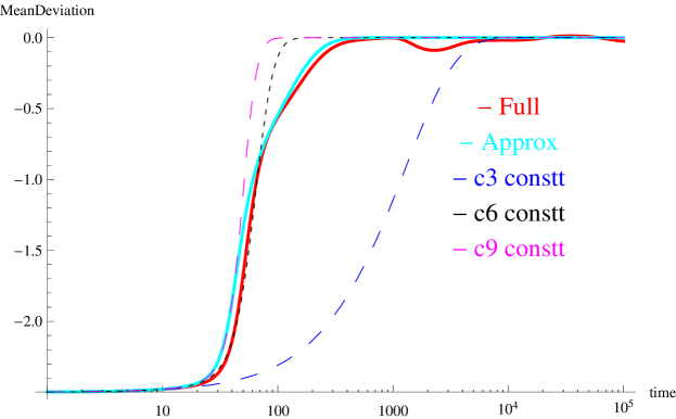
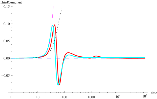
Figure S2: Dynamics of the cumulants when most effects are large: Numerical results obtained by closing the hierarchy in (13) when the third, sixth and ninth cumulants are assumed to be constant. Full and Approx refer to results obtained using the full model (6) and directional selection model (10). The parameters are the same as in Fig. 3.

$\alpha$	$\beta$	Integral $J_{l}$
20	0.1	0.00646802
	0.5	0.00782825
	1	0.0132363
	2	0.108583
	3	0.313421
	4	0.506622
	5	0.650011
	6	0.74967
200	0.1	0.000120827
	0.5	0.000135405
	1	0.000201675
	2	0.00935999
	3	0.0704926
	4	0.181047
	5	0.304219
	6	0.417745
2000	0.1	$1.78243\times 10^{-6}$
	0.5	$1.92926\times 10^{-6}$
	1	$2.6638\times 10^{-6}$
	2	0.000880179
	3	0.0160675
	4	0.0635073
	5	0.137642
	6	0.223307

Table S2: Numerical evaluation of the integral $J_{l}$ defined by (F.8) for various $\alpha$ and $\beta$.

References

- Abramowitz and Stegun (1964) Abramowitz, M. and I. A. Stegun, 1964 Handbook of Mathematical Functions with Formulas, Graphs, and Mathematical Tables. Dover.
- Arfken (1985) Arfken, G., 1985 Mathematical Methods for Physicists. Academic Press, New York.
- Axelsson et al. (2013) Axelsson, E., A. Ratnakumar, M. L. Arendt, K. Maqbool, M. T. Webster, M. Perloski, O. Liberg, J. M. Arnemo, A. Hedhammar, and K. Lindblad-Toh, 2013 The genomic signature of dog domestication reveals adaptation to a starch-rich diet. Nature 495: 360–364.
- Barton (1986) Barton, N. H., 1986 The maintenance of polygenic variation through a balance between mutation and stabilizing selection. Genet. Res. 47: 209–216.
- Barton and de Vladar (2009) Barton, N. H. and H. P. de Vladar, 2009 Statistical Mechanics and the Evolution of Polygenic Quantitative Traits. Genetics 181: 997–1011.
- Barton and Turelli (1991) Barton, N. H. and M. Turelli, 1991 Natural and sexual selection on many loci. Genetics 127: 229–255.
- Bod’ová et al. (2016) Bod’ová, K., G. Tkacik, and N. H. Barton, 2016 A general approximation for the dynamics of quantitative traits. Genetics 202: 1523–1548.
- Bürger (1991) Bürger, R., 1991 Moments, cumulants, and polygenic dynamics. J. Math. Biol. 30: 199–213.
- Bürger (2000) Bürger, R., 2000 The Mathematical Theory of Selection, Recombination, and Mutation. Wiley, Chichester.
- Castellani and Cavagna (2005) Castellani, T. and A. Cavagna, 2005 Spin-glass theory for pedestrians. J. Stat. Mech.:Theo. and Exp. 2005: P05012.
- Charlesworth (2013) Charlesworth, B., 2013 Stabilizing selection, purifying selection, and mutational bias in finite populations. Genetics 194: 955–971.
- Charlesworth and Charlesworth (2010) Charlesworth, B. and D. Charlesworth, 2010 Elements of evolutionary genetics. Roberts and Company Publishers.
- Chevin and Hospital (2008) Chevin, L.-M. and F. Hospital, 2008 Selective sweep at a quantitative trait locus in the presence of background genetic variation. Genetics 180: 1645–1660.
- Cook et al. (2012) Cook, L. M., B. S. Grant, I. J. Saccheri, and J. Mallet, 2012 Selective bird predation on the peppered moth: the last experiment of Michael Majerus. Biology Letters 8: 609–612.
- Coop et al. (2010) Coop, G., D. Witonsky, A. Di Rienzo, and J. K. Pritchard, 2010 Using environmental correlations to identify loci underlying local adaptation. Genetics 185: 1411–1423.
- de Vladar and Barton (2014) de Vladar, H. P. and N. H. Barton, 2014 Stability and response of polygenic traits to stabilizing selection and mutation. Genetics 197: 749–767.
- Ffrench-Constant et al. (2002) Ffrench-Constant, R. H., M. Bogwitz, P. Daborne, and J. Yen, 2002 A single P450 allele associated with insecticide resistance in Drosophila. Science 27: 2253–2256.
- Foll and Gaggiotti (2008) Foll, M. and O. Gaggiotti, 2008 A genome-scan method to identify selected loci appropriate for both dominant and codominant markers: a Bayesian perspective. Genetics 180: 977–993.
- Goddard and Hayes (2009) Goddard, M. E. and B. J. Hayes, 2009 Mapping genes for complex traits in domestic animals and their use in breeding programmes. Nat. Rev. Genet. 10: 381–391.
- Gomulkiewicz et al. (2010) Gomulkiewicz, R., R. D. Holt, M. Barfield, and S. L. Nuismer, 2010 Genetics, adaptation, and invasion in harsh environments. Evolutionary Applications 3: 97–108.
- Grant and Grant (2008) Grant, P. R. and B. R. Grant, 2008 How and Why Species Multiply: The Radiation of Darwin s Finches. Princeton NJ: Princeton University Press.
- Jain and Stephan (2015) Jain, K. and W. Stephan, 2015 Response of polygenic traits under stabilising selection and mutation when loci have unequal effects. G3: Genes, Genomes, Genetics 5: 1065–1074.
- Kaplan et al. (1989) Kaplan, N. L., R. R. Hudson, and C. H. Langley, 1989 The “hitchhiking effect” revisited. Genetics 123: 887–899.
- Kim and Stephan (2002) Kim, Y. and W. Stephan, 2002 Detecting a local signature of genetic hitchhiking along a recombining chromosome. Genetics 160: 765–777.
- Lamichhaney et al. (2015) Lamichhaney, S., J. Berglund, M. S. Almén, K. Maqbool, M. Grabherr, A. Martinez-Barrio, M. Promerová, C. J. Rubin, C. Wang, N. Zamani, B. R. Grant, P. R. Grant, M. T. Webster, and L. Andersson, 2015 Evolution of Darwin’s finches and their beaks revealed by genome sequencing. Nature 518: 371–375.
- Lamichhaney et al. (2012) Lamichhaney, S., A. Martinez Barrio, N. Rafati, G. Sundström, C. J. Rubin, E. R. Gilbert, J. Berglund, A. Wetterbom, L. Laikre, M. T. Webster, M. Grabherr, N. Ryman, and L. Andersson, 2012 Population-scale sequencing reveals genetic differentiation due to local adaptation in Atlantic herring. Proc. Natl. Acad. Sci. USA 109: 19345–19350.
- Lande (1976) Lande, R., 1976 Natural selection and random genetic drift in phenotypic evolution. Evolution 30: 314–334.
- Lande (1983) Lande, R., 1983 The response to selection on major and minor mutations affecting a metrical trait. Heredity 50: 47–65.
- Linnen et al. (2013) Linnen, C. R., Y. P. Poh, B. K. Peterson, R. D. Barrett, J. G. Larson, J. D. Jensen, and H. E. Hoekstra, 2013 Adaptive evolution of multiple traits through multiple mutations at a single gene. Science 339: 1312–1316.
- Losos (2009) Losos, J. B., 2009 Lizards in an Evolutionary Tree: Ecology and Adaptive Radiation of Anoles. San Francisco, CA: University of California Press.
- Losos (2014) Losos, J. B., 2014 What Darwin got wrong. Chronicle of Higher Education -: B13–B15.
- Mackay (2004) Mackay, T. F. C., 2004 The genetic architecture of quantitative traits: lessons from Drosophila. Current Opinion in Genetics and Development 14: 253–257.
- Matuszewski et al. (2015) Matuszewski, S., J. Hermisson, and M. Kopp, 2015 Catch me if you can: adaptation from standing genetic variation to a moving phenotypic optimum. Genetics 200: 1255–1274.
- Maynard Smith and Haigh (1974) Maynard Smith, J. and J. Haigh, 1974 Hitchhiking effect of a favourable gene. Genet. Res. 23: 23–35.
- Nielsen et al. (2005) Nielsen, R., S. Williamson, Y. Kim, M. J. Hubisz, A. G. Clark, and C. Bustamante, 2005 Genomic scans for selective sweeps using SNP data. Genome Res. 15: 1566–1575.
- Pavlidis et al. (2010) Pavlidis, P., J. D. Jensen, and W. Stephan, 2010 Searching for footprints of positive selection in whole-genome SNP data from nonequilibrium populations. Genetics 185: 907–922.
- Pavlidis et al. (2012) Pavlidis, P., D. Metzler, and W. Stephan, 2012 Selective sweeps in multilocus models of quantitative traits. Genetics 192: 225–239.
- Pritchard and Di Rienzo (2010) Pritchard, J. K. and A. Di Rienzo, 2010 Adaptation - not by sweeps alone. Nature Review Genetics 11: 665–667.
- Reznick (2009) Reznick, D. N., 2009 The Origin Then and Now: An Interpretive Guide to the Origin of Species. Princeton NJ: Princeton University Press.
- Riebler et al. (2008) Riebler, A., L. Held, and W. Stephan, 2008 Bayesian variable selection for detecting adaptive genomic differences among populations. Genetics 178: 1817–1829.
- Rubin et al. (2012) Rubin, C. J., H. J. Megens, A. Martinez Barrio, K. Maqbool, S. Sayyab, D. Schwochow, C. Wang, Ö. Carlborg, P. Jern, C. B. Jørgensen, A. L. Archibald, M. Fredholm, M. A. Groenen, and L. Andersson, 2012 Strong signatures of selection in the domestic pig genome. Proc. Natl. Acad. Sci. USA 109: 19529–19536.
- Sornette (2000) Sornette, D., 2000 Critical Phenomena in Natural Sciences. Springer, Berlin.
- Stephan et al. (1992) Stephan, W., T. H. E. Wiehe, and M. W. Lenz, 1992 The effect of strongly selected substitutions on neutral polymorphism: analytical results based on diffusion theory. Theor. Pop. Biol. 41: 237–254.
- Svetec et al. (2011) Svetec, N., A. Werzner, R. Wilches, P. Pavlidis, J. M. Alvarez-Castro, K. W. Broman, D. Metzler, and W. Stephan, 2011 Identification of X-linked quantitative trait loci affecting cold tolerance in Drosophila melanogaster and fine mapping by selective sweep analysis. Mol Ecol. 20: 530–544.
- Turchin et al. (2012) Turchin, M. C., C. W. K. Chiang, C. D. Palmer, S. Sankararaman, D. Reich, and J. Hirschhorn, 2012 Evidence of widespread selection on standing variation in Europe at height-associated SNPs. Nat. Genet. 44: 1015–1019.
- van’t Hof et al. (2011) van’t Hof, A. E., N. Edmonds, M. Daliková, F. Marec, and I. J. Saccheri, 2011 Industrial melanism in British peppered moths has a singular and recent mutational origin. Science 332: 958–960.
- Vignieri et al. (2010) Vignieri, S. N., J. G. Larson, and H. E. Hoekstra, 2010 The selective advantage of crypsis in mice. Evolution 64: 2153–2158.
- Visscher et al. (2012) Visscher, P. M., M. A. Brown, M. I. McCarthy, and J. Yang, 2012 Five years of GWAS discovery. Am J Hum Genet. 90: 7–24.
- Wilches et al. (2014) Wilches, R., S. Voigt, P. Duchen, S. Laurent, and W. Stephan, 2014 Fine-mapping and selective sweep analysis of QTL for cold tolerance in Drososphila melanogaster. G3: Genes, Genomes, Genetics 4: 1635–1645.
- Wollstein and Stephan (2014) Wollstein, A. and W. Stephan, 2014 Adaptive fixation in two-locus models of stabilizing selection and genetic drift. Genetics 198: 685–697.
- Wright (1935) Wright, S., 1935 Evolution in populations in approximate equilibrium. J. Genet. 30: 257–266.
File S1