Simulation of electrical machines – A FEM-BEM coupling scheme

Abstract.

Electrical machines commonly consist of moving and stationary parts. The field simulation of such devices can be very demanding if the underlying numerical scheme is solely based on a domain discretization, such as in case of the Finite Element Method (FEM). Here, a coupling scheme based on FEM together with Boundary Element Methods (BEM) is presented that neither hinges on re-meshing techniques nor deals with a special treatment of sliding interfaces. While the numerics are certainly more involved the reward is obvious: The modeling costs decrease and the application engineer is provided with an easy-to-use, versatile, and accurate simulation tool.

1. Introduction

Today’s development cycles of electric machines, magnetic sensors, or transformers are intimately connected with numerical simulation. A cost-effective development and optimization of these devices is hardly viable without virtual prototyping. The fundamentals of electromagnetic simulations are the Maxwell’s equations and one of the most popular and most versatile numerical discretization schemes is the Finite Element Method (FEM). While originally applied to problems in structural mechanics the FEM succeeded also for electromagnetic problems for more than 30 years.

However, the simplicity of the FEM does not come for free. Since electric and magnetic fields extend into the unbounded exterior air region one typically introduces homogeneous boundary conditions some distance away from the solid parts. Then by expanding the Finite Element grid to parts of the air region an approximation for the unknown fields can be obtained. Thanks to the decay properties of the electromagnetic fields this approach is widely applied, accepted, and justified for many applications. Nevertheless, some problems remain:

• Non-physical boundary conditions are imposed on the domain’s (fictitious) boundary and the introduced modeling error leads to contaminated solutions. This might become critical when highly accurate simulation results are needed.

• The meshing of the air region requires a considerable amount of time and effort. In many situations the number of elements in the air region even exceeds the number of elements used for the solid parts.

• Electrical devices often contain moving parts. For instance, the variation of the rotor/stator positions of an electric motor requires either a re-meshing of the air gap or a fundamental modification of the Finite Element scheme.

• The accurate computation of electro-mechanical forces with a FEM-only discretization remains a challenge.

In this work we are going to present the implementation of a FEM-BEM coupling scheme in which the air region is handled by the Boundary Element Method (BEM) while only the solid parts are discretized by the FEM. The BEM is a convenient tool to tackle unbounded exterior domains and it is well-designed to eliminate the above mentioned problems. The method is based on the discretization of Boundary Integral Equations (BIEs) [10] that are defined on the surface of the computational domain. Hence, no meshing is required for the air region. Further, the BIEs fulfill the decay and radiation conditions of the electromagnetic fields such that no additional modeling errors occur. And finally, a simple, automatic treatment of moving parts is intrinsic to the presented scheme. The force computation is beyond the scope of this paper but it is important to note that the BEM computations provide us with additional information such that these calculations can be carried out with unparalleled accuracy.

This work is organized as follows: Section 2 recalls the main idea of the FEM-BEM coupling. The coupling relies mainly on the theoretical work presented in [7]. For proper definitions of the mathematical spaces, their traces, and the occurring surface differential operators we refer to that publication and to the references cited therein. In section 3 the method itself and the presented preconditioning strategy are verified. Additionally, applications to industrial models are presented, where we remark on the incorporation of periodic constraints. Finally, this work closes with a conclusion in section 4.

2. Symmetric FEM-BEM Coupling

We summarize the FEM-BEM coupling scheme as it has been proposed in [7]. The governing equations for magnetostatics are

(1) $$\operatorname{div}\mathbf{B}=0\,,\quad\operatorname{\mathbf{curl}}\mathbf{H}=\mathbf{j}\,,\quad\mathbf{B}=\mu\left(\mathbf{H}+\mathbf{M}\right)\;.$$

The first equation is Gauss’s law for magnetism, the second equation is Ampéres law in differential form, and the third equation is the material law. It connects the magnetic flux $\mathbf{B}$ with the magnetic field $\mathbf{H}$ via the – possibly non-linear – magnetic permeability $\mu$. The prescribed quantities are the solenoidal excitation current, $\mathbf{j}$, and a given magnetization $\mathbf{M}$. By introducing the non-gauged vector potential $\mathbf{A}$ such that $\operatorname{\mathbf{curl}}\mathbf{A}\coloneqq\mathbf{B}$ the following variational formulation holds:

Find $\mathbf{A}\in H(\operatorname{\mathbf{curl}},{\Omega^{-}})$ such that

(2) $$\langle\mu^{-1}\operatorname{\mathbf{curl}}\mathbf{A},\operatorname{\mathbf{curl}}\mathbf{A}^{\prime}\rangle_{\Omega^{-}}-\langle\mu^{-1}{\gamma_{N}^{-}}\mathbf{A},{\gamma_{D}^{-}}\mathbf{A}^{\prime}\rangle_{\Gamma}=\\ \langle\mathbf{j},\mathbf{A}^{\prime}\rangle_{\Omega^{-}}+\langle\mathbf{M},\operatorname{\mathbf{curl}}\mathbf{A}^{\prime}\rangle_{\Omega^{-}}$$

for all test-functions $\mathbf{A}^{\prime}\in H(\operatorname{\mathbf{curl}},{\Omega^{-}})$.

Above, we have used the notation $\langle\mathbf{u},\mathbf{w}\rangle_{M}\coloneqq\int_{M}\mathbf{u}\cdot\mathbf{w}\,\operatorname{d}\!M$. The interior domain is ${\Omega^{-}}\subset\mathbb{R}^{3}$ and $\Gamma\coloneqq\partial{\Omega^{-}}$ is its boundary. The complementary unbounded exterior air region is given by ${\Omega^{+}}=\mathbb{R}^{3}\setminus\overline{{\Omega^{-}}}$. The space $H(\operatorname{\mathbf{curl}},{\Omega^{-}})$ denotes the space of square integrable vector functions with a square integrable curl [13]. Further, $\gamma$ denotes the trace operator. The Dirichlet and Neumann traces for the interior as well as for the exterior domain are given by

(3) $$\gamma^{\pm}_{D}\mathbf{A} \coloneqq\lim_{\Omega^{\pm}\ni\tilde{\mathbf{x}}\to\mathbf{x}\in\Gamma}\mathbf{n}(\mathbf{x})\times(\mathbf{A}(\tilde{\mathbf{x}})\times\mathbf{n}(\mathbf{x}))$$

$$\gamma^{\pm}_{N}\mathbf{A} \coloneqq\lim_{\Omega^{\pm}\ni\tilde{\mathbf{x}}\to\mathbf{x}\in\Gamma}\operatorname{\mathbf{curl}}_{\tilde{\mathbf{x}}}\mathbf{A}(\tilde{\mathbf{x}})\times\mathbf{n}(\mathbf{x})$$

with $\mathbf{n}$ being the normal vector outward to ${\Omega^{-}}$. Schemes that rely solely on Finite Element Methods commonly neglect the boundary term in (2), i.e., either ${\gamma_{N}^{-}}\mathbf{A}$ or ${\gamma_{D}^{-}}\mathbf{A}^{\prime}$ are ignored such that the variational formulation corresponds to a homogeneous Neumann- or Dirichlet-problem, respectively. However, in a coupled formulation the interior traces are expressed by their exterior counterparts via appropriate transmission conditions. For the given physical model, these transmission conditions read

(4) $${\gamma_{D}^{-}}\mathbf{A}={\gamma_{D}^{+}}\mathbf{A}\qquad\mu^{-1}{\gamma_{N}^{-}}\mathbf{A}=\mu_{0}^{-1}{\gamma_{N}^{+}}\mathbf{A}$$

with $\mu_{0}$ denoting the vacuum permeability. The vector potential $\mathbf{A}$ fulfills the following representation formula [3, Ch. 6.2]

(5) $$\mathbf{A}(\tilde{\mathbf{x}})= \int_{\Gamma}U(\tilde{\mathbf{x}}-\mathbf{y})\,{\gamma_{N}^{+}}\mathbf{A}(\mathbf{y})\,\operatorname{d}\!s_{\mathbf{y}}$$

$$-\operatorname{\mathbf{curl}}_{\tilde{\mathbf{x}}}\int_{\Gamma}U(\tilde{\mathbf{x}}-\mathbf{y})\,(\mathbf{n}\times\mathbf{A})(\mathbf{y})\,\operatorname{d}\!s_{\mathbf{y}}$$

$$+\operatorname{\mathbf{grad}}_{\tilde{\mathbf{x}}}S(\mathbf{A})$$

for all points $\tilde{\mathbf{x}}\in\Omega^{+}$, $\mathbf{y}\in\Gamma$, and with $U(\tilde{\mathbf{x}}-\mathbf{y})\coloneqq\nicefrac{{1}}{{4\pi|\tilde{\mathbf{x}}-\mathbf{y}|}}$ being the fundamental solution for the Laplace operator. The last term in (5) is

(6) $$S(\mathbf{A})\coloneqq\int_{\Gamma}U(\tilde{\mathbf{x}}-\mathbf{y})\,(\mathbf{n}\cdot\mathbf{A})(\mathbf{y})\,\operatorname{d}\!s_{\mathbf{y}}\;.$$

Applying the traces ${\gamma_{D}^{+}}$, and ${\gamma_{N}^{+}}$ to (5) we arrive at the set of weak boundary integral equations

(7) $$\langle\gamma_{D}^{+}\mathbf{A},\boldsymbol{\zeta}\rangle_{\Gamma} =\langle\mathbf{K}(\gamma_{D}^{+}\mathbf{A}),\boldsymbol{\zeta}\rangle_{\Gamma}-\langle\mathbf{V}(\gamma_{N}^{+}\mathbf{A}),\boldsymbol{\zeta}\rangle_{\Gamma}$$

$$\langle\gamma_{N}^{+}\mathbf{A},\mathbf{w}\rangle_{\Gamma} =\langle\mathbf{N}(\gamma_{D}^{+}\mathbf{A}),\mathbf{w}\rangle_{\Gamma}-\langle\mathbf{K}^{*}(\gamma_{N}^{+}\mathbf{A}),\mathbf{w}\rangle_{\Gamma}\;.$$

Above, $\mathbf{V}$ denotes the Maxwell single layer potential, $\mathbf{N}$ is the hypersingular operator, and $\mathbf{K}$, $\mathbf{K}^{*}$ are the Maxwell double layer potential and its adjoint, respectively

(8) $$\mathbf{V}({\gamma_{N}^{+}}\mathbf{A}) \coloneqq\gamma_{D}^{+}\boldsymbol{\psi}_{\mathbf{A}}({\gamma_{N}^{+}}\mathbf{A}) \qquad\mathbf{K}({\gamma_{D}^{+}}\mathbf{A}) \coloneqq\gamma_{D}^{+}\boldsymbol{\psi}_{\mathbf{M}}({\gamma_{D}^{+}}\mathbf{A})$$

$$\mathbf{K}^{*}({\gamma_{N}^{+}}\mathbf{A}) \coloneqq\gamma_{N}^{+}\boldsymbol{\psi}_{\mathbf{A}}({\gamma_{N}^{+}}\mathbf{A}) \qquad\mathbf{N}({\gamma_{D}^{+}}\mathbf{A}) \coloneqq\gamma_{N}^{+}\boldsymbol{\psi}_{\mathbf{M}}({\gamma_{D}^{+}}\mathbf{A})\;.$$

The potentials $\boldsymbol{\psi}_{\mathbf{A}}$ and $\boldsymbol{\psi}_{\mathbf{M}}$ read

(9) $$(\boldsymbol{\psi}_{\mathbf{A}}\mathbf{u})(\tilde{\mathbf{x}}) \coloneqq\int_{\Gamma}U(\tilde{\mathbf{x}}-\mathbf{y})\,\mathbf{u}(\mathbf{y})\,\operatorname{d}\!s_{\mathbf{y}}$$

$$(\boldsymbol{\psi}_{\mathbf{M}}\mathbf{v})(\tilde{\mathbf{x}}) \coloneqq\operatorname{\mathbf{curl}}_{\tilde{\mathbf{x}}}\boldsymbol{\psi}_{\mathbf{A}}(\mathbf{n}\times\mathbf{v})(\tilde{\mathbf{x}})$$

for all points $\tilde{\mathbf{x}}\notin\Gamma$. For further informations on the above introduced boundary integral operators we refer to [7]. Eqn. (7) holds for $\boldsymbol{\zeta}\in H(\operatorname{\operatorname{div}_{\Gamma}}0,\Gamma)\subset H(\operatorname{\operatorname{div}_{\Gamma}},\Gamma)$ and $\mathbf{w}\in H(\operatorname{\operatorname{curl}_{\Gamma}},\Gamma)$. While $\mathbf{w}$ is an element of the trace space of $H(\operatorname{\mathbf{curl}},{\Omega^{-}})$, the function $\boldsymbol{\zeta}$ is taken from the space of vector fields with vanishing surface divergence, i.e., $\operatorname{\operatorname{div}_{\Gamma}}\boldsymbol{\zeta}\equiv 0$. The use of this special space is motivated by the fact that the potential in (6) has no physical meaning within this physical context and, therefore, shall be removed from the final numerical scheme. Because of $\operatorname{\mathbf{curl}}\operatorname{\mathbf{grad}}S\equiv 0$ the potential drops out naturally when the Neumann trace is applied to (5). Contrary, for the Dirichlet trace it vanishes only in the weak setting. Integration by parts then gives

(10) $$\langle\gamma_{D}^{+}\operatorname{\mathbf{grad}}_{\tilde{\mathbf{x}}}S(\mathbf{A}),\boldsymbol{\zeta}\rangle_{\Gamma}=\langle\operatorname{\mathbf{grad}}_{\Gamma}S(\mathbf{A}),\boldsymbol{\zeta}\rangle_{\Gamma}=-\langle S(\mathbf{A}),\operatorname{\operatorname{div}_{\Gamma}}\boldsymbol{\zeta}\rangle_{\Gamma}=0\;.$$

Due to $\operatorname{\operatorname{div}_{\Gamma}}\operatorname{\mathbf{curl}}_{\Gamma}\varphi\equiv 0$ the divergence-free constraint can be imposed via the surface rotation $\operatorname{\mathbf{curl}}_{\Gamma}$ of some continuous scalar function $\varphi$. Let $\boldsymbol{\lambda}\coloneqq{\gamma_{N}^{+}}\mathbf{A}$ abbreviate the exterior Neumann trace. We then define the vector field

(11) $$\boldsymbol{\lambda}\coloneqq\operatorname{\mathbf{curl}}_{\Gamma}\varphi\,,\quad\varphi\in H^{1/2}(\Gamma)\;.$$

Using the transmission conditions (4), the variational formulations (2) and (7) are combined. Introducing the relative permeability $\mu_{r}\coloneqq\nicefrac{{\mu}}{{\mu_{0}}}$ together with ${\gamma_{D}^{-}}={\gamma_{D}^{+}}\eqqcolon{\gamma_{D}}$, the coupled variational form reads: Find $\mathbf{A}\in H(\operatorname{\mathbf{curl}},{\Omega^{-}})$, $\varphi\in H^{1/2}(\Gamma)$ such that

(12) $$\langle\mu^{-1}_{r}\operatorname{\mathbf{curl}}\mathbf{A},\operatorname{\mathbf{curl}}\mathbf{A}^{\prime}\rangle_{\Omega^{-}}-\langle\mathbf{N}({\gamma_{D}}\mathbf{A}),{\gamma_{D}}\mathbf{A}^{\prime}\rangle_{\Gamma}+ \langle\mathbf{K}^{*}\operatorname{\mathbf{curl}}_{\Gamma}\varphi,{\gamma_{D}}\mathbf{A}^{\prime}\rangle_{\Gamma}$$

$$=\mu_{0}\langle\mathbf{j} ,\mathbf{A}^{\prime}\rangle_{\Omega^{-}}+\mu_{0}\langle\mathbf{M},\operatorname{\mathbf{curl}}\mathbf{A}^{\prime}\rangle_{\Omega^{-}}$$

$$\langle\left(\mathbf{K}-\mathbf{Id}\right)({\gamma_{D}}\mathbf{A}),\operatorname{\mathbf{curl}}_{\Gamma}\psi\rangle_{\Gamma}-\langle\mathbf{V}\operatorname{\mathbf{curl}}_{\Gamma}\varphi ,\operatorname{\mathbf{curl}}_{\Gamma}\psi\rangle_{\Gamma}=0$$

for all functions $\mathbf{A}^{\prime}\in H(\operatorname{\mathbf{curl}},{\Omega^{-}})$, $\psi\in H^{1/2}(\Gamma)$. Note that the variational form (12) is symmetric because of

(13) $$\langle\mathbf{K}^{*}\boldsymbol{\lambda},\mathbf{w}\rangle_{\Gamma}=\langle(\mathbf{K}-\mathbf{Id})\mathbf{w},\boldsymbol{\lambda}\rangle_{\Gamma}$$

for all $\mathbf{w}\in H(\operatorname{\operatorname{curl}_{\Gamma}},\Gamma)$, $\boldsymbol{\lambda}\in H(\operatorname{\operatorname{div}_{\Gamma}}0,\Gamma)$ [7].

Next, a geometrically conformal triangulation $\overline{\Omega_{h}}\coloneqq\cup_{n=1}^{N}K_{n}\approx{\Omega^{-}}$ is introduced. The $N$ mesh elements $K_{n}$ may consist of tetrahedra, hexahedra, prisms, and pyramids. Additionally, this triangulation induces a surface mesh $\Gamma_{h}$ of $\Gamma$ composed of triangles and/or quadrilaterals. Nédélec elements [14, 2] are used for a conformal discretization of $H(\operatorname{\mathbf{curl}},{\Omega^{-}})$. The linear system corresponding to (12) then reads

(14) $$S\underline{x}=\underline{g}$$

with

(15) $$S=\begin{bmatrix}A+R^{\top}NR&R^{\top}K^{\top}G\\ G^{\top}KR&-G^{\top}VG\end{bmatrix},\,\underline{x}=\begin{bmatrix}\underline{a}\\ \underline{\varphi}\end{bmatrix},\,\underline{g}=\begin{bmatrix}\underline{f}\\ 0\end{bmatrix}\,.$$

Above, $A$ is the matrix corresponding to the discretization of the $\operatorname{\mathbf{curl}}$-operator (see Eqn. (2)), and $N$, $K$, and $V$ are matrix representations of the formerly introduced BEM-operators. The given right hand side is $\underline{f}=\underline{f}(\mathbf{j};\mathbf{M})$ and it represents the right hand side terms of the first equation in (12). Fast Boundary Element Methods are utilized in order to obtain data sparse representations of the originally dense BEM matrices [5, 4]. Their use is mandatory since they reduce the quadratic complexity $O(N^{2})$ of the Boundary Element Method to quasi-linear costs $O(N\log N)$ or even to linear costs $O(N)$, respectively. It remains to comment on the matrices $R$ and $G$, respectively. In (15), $R$ is a restriction matrix that extracts the boundary coefficients. The matrix $G$ maps the surface curls of piecewise linear continuous functions to elements of $H(\operatorname{\operatorname{div}_{\Gamma}},\Gamma)$. It is sometimes denoted as topological gradient [6, Ch. 3]. The entries of $G$ are given by $G[\ell,k]=\pi_{\ell}(\operatorname{\mathbf{curl}}_{\Gamma}\varphi_{k})$. Here, $\pi_{\ell}$ denotes the functional that defines the degrees of freedom for the Raviart-Thomas element which is used for the discretization of $H(\operatorname{\operatorname{div}_{\Gamma}},\Gamma)$ [17]. For the lowest order space this functional is $\pi_{\ell}(\mathbf{v})\coloneqq\int_{E_{\ell}}\left(\mathbf{n}\times\mathbf{v}\right)\cdot\operatorname{d}\!\mathbf{s}$ with $E_{\ell}$ being the $\ell$-th edge of the surface mesh $\Gamma_{h}$.

\begin{overpic}[width=216.81pt]{torus_mesh} \footnotesize\put(69.0,25.0){$\gamma_{1}^{\prime}$} \put(50.0,14.0){$\gamma_{1}$} \end{overpic}

Figure 1. Torus with its generating cycles $\gamma_{1}$ and $\gamma_{1}^{\prime}$

The construction of the numerical scheme is almost complete. However, one challenge remains: In most applications, the interior domain ${\Omega^{-}}$ is non-simply connected. The torus in Fig. 1 depicts such a domain since the two loops $\gamma_{1}^{\prime}$ and $\gamma_{1}$ cannot be contracted on the surface to a point. The definition (11) introduces a scalar potential for the exterior domain such that we have $\mathbf{H}^{+}=-\operatorname{\mathbf{grad}}\varphi$ for the exterior magnetic field. Let $\Sigma$ be some oriented cross section area and $\gamma=\partial\Sigma$ a closed path. The integral form of Ampére’s law is

(16) $$\oint_{\gamma}\mathbf{H}^{+}\cdot\operatorname{d}\!\boldsymbol{\ell}=\int_{\Sigma}\mathbf{j}\cdot\operatorname{d}\!\boldsymbol{\Sigma}=I$$

with the total current density $I$. We assume that the torus in Fig. 1 features a total current density $I\neq 0$. Obviously Ampére’s law is violated if the path $\gamma^{\prime}_{1}$ is chosen. In this case the path integral of the gradient field evaluates to zero. This contradicts (16) and the choice (11) has to be augmented

(17) $$\boldsymbol{\lambda}\coloneqq\operatorname{\mathbf{curl}}_{\Gamma}\varphi+\sum_{m=1}^{M}\alpha_{m}\boldsymbol{\eta}_{m}\;.$$

In (17), the functions $\boldsymbol{\eta}_{m}\in H(\operatorname{\operatorname{div}_{\Gamma}}0,\Gamma)$ are current sheets along paths $\gamma_{m}$. They feature the jump

(18) $$\oint_{\gamma_{m}^{\prime}}(\mathbf{n}\times\boldsymbol{\eta}_{m})\cdot\operatorname{d}\!\boldsymbol{\ell}=1$$

across the path $\gamma_{m}$. The number $M$ of relevant paths is given by the number of holes drilled through ${\Omega^{-}}$. An algorithm for the construction of these paths can be found in [8]. Inserting (17) into the variational form (12) results in the modified system

(19) $$\begin{bmatrix}S&F_{\boldsymbol{\eta}}\\ F^{\top}_{\boldsymbol{\eta}}&H_{\boldsymbol{\eta}}\end{bmatrix}\cdot\begin{bmatrix}\underline{x}\\ \underline{\alpha}\end{bmatrix}=\begin{bmatrix}\underline{g}\\ 0\end{bmatrix}\;.$$

With $S_{\boldsymbol{\eta}}\coloneqq F_{\boldsymbol{\eta}}H_{\boldsymbol{\eta}}^{-1}F^{\top}_{\boldsymbol{\eta}}$, (19) can alternatively be written as

(20) $$\widehat{S}\underline{x}=\underline{g}\,,\quad\widehat{S}\coloneqq S-S_{\boldsymbol{\eta}}\;.$$

The matrix $S_{\boldsymbol{\eta}}$ is a $\operatorname{rank}(M)$ perturbation of the original system (14). Since $M\ll\dim(S)$, this perturbation does not significantly alter the spectral properties of $S$. Hence, the upcoming preconditioning strategy neglects the influence of $S_{\boldsymbol{\eta}}$.

The linear system (14) is symmetric but not positive definite. We therefore apply a MINRES solver [16] to the preconditioned system. The block preconditioner is given by $P_{S}^{-1}=\operatorname{diag}(P^{-1}_{\text{AMS}},P^{-1}_{V})$ where $P^{-1}_{\text{AMS}}$ is an AMG/AMS preconditioner. This preconditioner is based on algebraic multigrid methods (AMG) as they have been developed for the discretization of Finite Element spaces like, e.g., $H^{1}(\Omega)$. However, since we are dealing with Nédélec-type Finite Element spaces the standard AMG preconditioners cannot be applied directly. An enhancement based on auxiliary space methods has been developed in [9]. It is denoted as auxiliary Maxwell space preconditioner (AMS) and appears to be the natural choice for magnetostatic and eddy-current problems. The BEM preconditioner $P^{-1}_{V}$ is based on operator preconditioning techniques [15]. Due to the use of hierarchical function spaces [2] (cf. Fig. 2), subspace correction methods are used in case of higher order schemes [18].

Figure 2. Hierarchical functions on the triangle. Upper row: $2^{\text{nd}}$ and $3^{\text{rd}}$ order functions for $H^{1/2}(\Gamma)$. Lower row: $1^{\text{st}}$ and $2^{\text{nd}}$ order functions for $H(\operatorname{\operatorname{curl}_{\Gamma}},\Gamma)$.

3. Numerical Examples

3.1. Verification

The numerical scheme is verified by means of an academic example. We consider a magnetized unit sphere, i.e., ${\Omega^{-}}\coloneqq\{\mathbf{x}\colon|\mathbf{x}|<1\}$. The sphere has a constant magnetization $\mathbf{M}=M_{0}\mathbf{e}_{3}$ in $x_{3}$-direction with $M_{0}=1$.

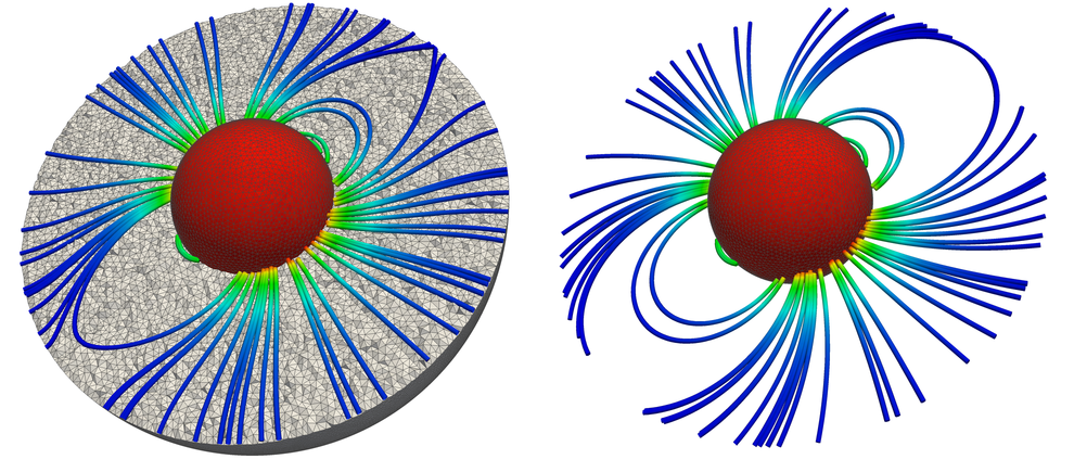
Figure 3. Comparison between FEM and FEM-BEM. Left: FEM solution $\mathbf{B}$ with field lines artificially normal to the boundary. Right: FEM-BEM solution shows correct behavior.

The analytic solution for the magnetic flux is $\mathbf{B}^{-}=\nicefrac{{2\mu_{0}}}{{3}}\mathbf{M}$ and $\varphi(\mathbf{x})=\nicefrac{{x_{3}}}{{3}}$ for the scalar potential [11, Ch. 5.10].

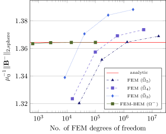
Figure 4. FEM-BEM on ${\Omega^{-}}$ vs. FEM on $\widehat{\Omega}_{R}$

In Fig. 4 the $L_{2}$-norms for the computed magnetic fluxes are compared against the analytic solution $\mu_{0}^{-1}\|\mathbf{B}^{-}\|_{2,\text{sphere}}=|\mathbf{B}^{-}|\sqrt{\operatorname{vol}({\Omega^{-}})}\approx 1.3644$. In addition, pure FEM computations have been taken out for various fictitious domains $\widehat{\Omega}_{R}\coloneqq{\Omega^{-}}\cup\{\mathbf{x}\colon 1\leq|\mathbf{x}|<R\}$ with homogeneous Neumann boundary conditions on $\partial\widehat{\Omega}_{R}$. Curved tetrahedral elements have been used for the experiments. Clearly, the modeling error prevents the FEM computations from converging to the correct result (cf. Fig. 3). Even $20$ millions of FEM degrees of freedoms (dofs) for the finest grid on $\widehat{\Omega}_{5}$ are outperformed by just 600 FEM dofs that are used within the FEM-BEM scheme for the coarsest grid on ${\Omega^{-}}$.

However, while the results from Fig. 4 are proving the correctness of the FEM-BEM formulation, the comparison with the FEM-only computations is slightly unfair. This is due to the nature of the analytic solution. It is constant for the magnetic flux within the sphere and linear for the scalar potential on the boundary. Both fields can be represented exactly by the used FE spaces. Hence, the errors for the FEM-BEM formulation in Fig. 4 are just due to the geometrical error induced by the triangulation. Therefore, in the following example the FEM-BEM scheme is not only applied to the magnetized sphere ${\Omega^{-}}$ but to the domain $\widehat{\Omega}_{4}$ that includes some air region. In this case the magnetic flux in the air region is given by $\mathbf{B}^{+}=-\mu_{0}M_{0}\operatorname{\mathbf{grad}}\tfrac{x_{3}}{3|\mathbf{x}|^{3}}$ which is not covered by the Finite Element spaces.

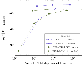
Figure 5. FEM-BEM on $\widehat{\Omega}_{4}$ vs. FEM on $\widehat{\Omega}_{5}$

Fig. 5 shows the results for the coupled scheme together with those for the pure FEM computations. Again, we notice that there is convergence towards the correct solution but now the geometric error is dominated by the approximation error. Since the lowest order FE spaces exhibit only linear convergence, higher order schemes are also exploited. Their use is highly beneficial: Even the results for the second coarsest grid reveal an accuracy that cannot be achieved by lowest order discretizations on any of the used grids.

3.2. Preconditioning

Now that the scheme has been verified, the performance of the preconditioner is investigated. In Fig. 6, a circular current loop surrounds a magnetic core. The model is discretized with three different grids (see Tab. 1).

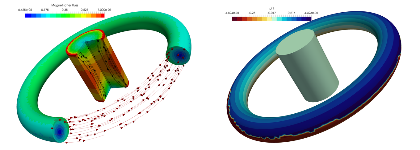
Figure 6. Left: Magnetic flux $\mathbf{B}$ and excitation current $\mathbf{j}$. Right: Potential $\varphi$ with jump across generating cycle.

Table 1. Discretizations

$L_{i}$	Mesh size	$N_{\text{FEM}}$	$N_{\text{BEM}}$
$1$	$0.60$	$5\,402$	$706$
$2$	$0.39$	$27\,251$	$2\,872$
$3$	$0.19$	$166\,748$	$12\,049$

In Tab. 2 the iteration numbers are given for the three refinement levels $L_{i}$ as well as for varying permeabilities $\mu_{r}$. The relative solver tolerance has been set to $\varepsilon_{r}=10^{-8}$. Obviously, the preconditioner is very effective since it reveals only a slight dependence on the mesh size and on the jumps of material coefficients.

Table 2. Iteration numbers

$\mu_{r}$	$L_{1}$	$L_{2}$	$L_{3}$
$10^{0}$	$47$	$51$	$63$
$10^{2}$	$78$	$88$	$117$
$10^{5}$	$84$	$92$	$119$

3.3. Periodicities

For industrial applications it is important to deal with models that feature geometrical periodicities. Fig. 7 shows a simple motor model that exploits periodicities. Only a sixth of the model has been discretized. While it is quite simple to impose periodic constraints into Finite Element schemes, the situation is a bit more complicated with Boundary Elements.

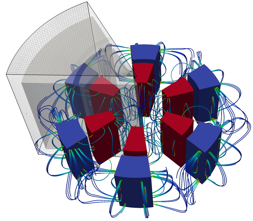
Figure 7. Device with periodicities. Magnetic flux $\mathbf{B}$. $1.5\cdot 10^{6}$ FEM-dofs and $1.4\cdot 10^{4}$ BEM-dofs

Fig. 8 sketches a model with periodicities. Due to the non-local kernel function $U(\mathbf{x}-\mathbf{y})$ interactions on domains $\Omega_{i}$, $i=1,\ldots,n$ with all other domains $\Omega_{j}$ occur. The resulting BEM matrix $V$ formally has $n\times n$ blocks $V_{i,j}$ but the periodicities render $V$ as block circulant matrix

(21) $$V=\begin{bmatrix}V_{1,1}&V_{1,2}&V_{1,3}&\dots&V_{1,n}\\ V_{1,n}&V_{1,1}&V_{1,2}&\dots&V_{1,n-1}\\ V_{1,n-1}&V_{1,n}&V_{1,1}&\dots&V_{1,n-2}\\ &\ddots&\ddots&\ddots&\\ V_{1,2}&V_{1,3}&V_{1,4}&\dots&V_{1,1}\end{bmatrix}\;.$$

Hence, only the matrices $V_{1,i}$, $i=1,\ldots,n$ need to be computed and stored.

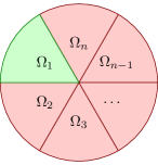
Figure 8. Periodicities

If we assume a periodic excitation, we get for the solution vector blocks $\underline{x}_{1}=\ldots=\underline{x}_{n}\eqqcolon\underline{x}$ and therefore the matrix-vector product (21) simplifies to

(22) $$\underline{y}=\sum_{i=1}^{n}V_{1,i}\,\underline{x}\;.$$

The above expression simplifies further if the properties of the Galerkin-scheme are taken into account. The BEM matrices in Eqn. (15) are symmetric and this symmetry reduces the complexity even further. In case of non-periodic excitations, techniques like the Fast Fourier Transform are exploited to define a fast matrix-vector product for the matrix (21). More information about the handling of periodicities can be found in [12, 1].

3.4. Magnetic valve with moving armature

Finally, Fig. 9 shows a magnetic valve that consists of approximately $2.4\cdot 10^{6}$ degrees of freedom in the FEM domain and of $1.1\cdot 10^{5}$ degrees of freedom for the BEM part. At its bottom the valve has a moving armature and the excitation is given by a circular current $\mathbf{j}$. The relative solver tolerance is set to $\varepsilon_{r}=10^{-6}$ and $236$ iterations are required to solve the system for the initial configuration (Fig. 9). Less iterations are then needed for the moving parts because the previous solution provides a good start vector.

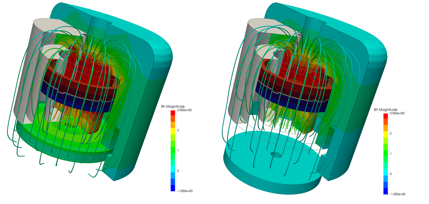
Figure 9. Moving armature: $\mathbf{B}$-field and scalar potential $\varphi$ on the toroidal coil. Note the jump of the scalar potential on the coil’s surface.

The magnetic valve, consists of three distinct components: The armature at its bottom, the toroidal coil, and the remaining composite components like, e.g., some permanent magnets and the housing. Thus, for $M$ distinct components the linear system (20) can be partitioned w.r.t. the $M$ domains

(23) $$\widehat{S}=\begin{bmatrix}\widehat{S}_{11}&\dots&\widehat{S}_{1m}\\ \vdots&\ddots&\vdots\\ \widehat{S}_{1m}^{\top}&\dots&\widehat{S}_{mm}\end{bmatrix}\,,\quad m=1,\dots,M\;.$$

The same holds for the preconditioner. The partitioned preconditioner is $P^{-1}_{S}=\operatorname{diag}(P^{-1}_{S_{11}},\ldots,P^{-1}_{S_{mm}})$. Hence, if one component $k$ changes its position, only the off-diagonal blocks $\widehat{S}_{km}$, $m=1,\dots,M$ with $m\neq k$ need to be updated while the preconditioner remains unchanged.

This simplicity in handling moving parts is a preeminent advantage for the presented FEM-BEM coupling. The application engineer is provided with maximal convenience without loss of accuracy during the modeling process.

4. Conclusion

This work presents an implementation of a FEM-BEM coupling scheme for electromagnetic field simulations. The coupling eliminates problems that are inherent to a pure FEM approach. In detail, the benefits of the FEM-BEM scheme are: The decay conditions are fulfilled exactly, no meshing of parts of the exterior air region is necessary, and – most importantly – the handling of moving parts is incorporated in an intriguingly simple fashion. As a downside, the coupling is considerably more complex than a pure Finite Element scheme: The use of Boundary Element Methods requires advanced compression techniques and the incorporation of non-simply connected domains demands further adoptions of the scheme. However, once these issues have been handled, the FEM-BEM formulation in conjunction with a state-of-the-art preconditioner demonstrates its potency. The numerical tests not only reveal an accurate convergence behavior but also prove the algorithm to be suitable for industrial applications – especially, if improvements such as the incorporation of periodicities and the handling of multiple domains are implemented.

Eventually, the presented FEM-BEM formulation is an expedient supplement to a pure FEM. While not intended to be used under all circumstances it represents a powerful tool in case that high accuracies together with simple mesh-handling facilities are required.

References

- [1] E. L. Allgower, K. Georg, R. Miranda, and J. Tausch, Numerical Exploitation of Equivariance, ZAMM - Journal of Applied Mathematics and Mechanics 78 (1998), no. 12, 795–806.
- [2] M. Bergot and M. Duruflé, High-order optimal edge elements for pyramids, prisms and hexahedra, Journal of Computational Physics 232 (2013), no. 1, 189–213.
- [3] D. Colton and R. Kress, Inverse acoustic and electromagnetic scattering theory, vol. 93, Springer Science & Business Media, 2012.
- [4] L. Greengard and V. Rokhlin, A new version of the Fast Multipole Method for the Laplace equation in three dimensions, Acta Numerica 6 (1997), 229–269.
- [5] W. Hackbusch, Hierarchische matrizen: Algorithmen und analysis, Springer-Verlag Berlin Heidelberg, 2009.
- [6] R. Hiptmair, Finite elements in computational electromagnetism, Acta Numerica 11 (2002), 237–339.
- [7] R. Hiptmair, Symmetric coupling for eddy current problems, SIAM Journal on Numerical Analysis 40 (2002), no. 1, 41–65.
- [8] R. Hiptmair and J. Ostrowski, Generators of for Triangulated Surfaces: Construction and Classification, SIAM Journal on Computing 31 (2002), no. 5, 1405–1423.
- [9] R. Hiptmair and J. Xu, Nodal auxiliary space preconditiong in H(curl) and H(div) spaces, SIAM Journal on Numerical Analysis 45 (2007), 2483–2509.
- [10] G.C. Hsiao and W.L. Wendland, Boundary integral equations, Applied mathematical sciences, Springer, 2008.
- [11] J. D. Jackson, Classical electrodynamics, 3rd ed., John Wiley & Sons, Inc., 1999.
- [12] S. Kurz, O. Rain, and S. Rjasanow, Application of the adaptive cross approximation technique for the coupled BE-FE solution of symmetric electromagnetic problems, Computational mechanics 32 (2003), no. 4-6, 423–429.
- [13] P. Monk, Finite element methods for maxwell’s equations, Oxford University Press, 2003.
- [14] J.C. Nédélec, Mixed finite elements in , Numerische Mathematik 35 (1980), 315–341.
- [15] G. Of, BETI-Gebietszerlegungsmethoden mit schnellen Randelementverfahren und Anwendungen, Ph.D. thesis, Institut für Angewandte Analysis und Numerische Simulation, Universität Stuttgart, 2006.
- [16] C. C. Paige and M. A. Saunders, Solution of sparse indefinite systems of linear equations, SIAM Journal on Numerical Analysis 12 (1975), no. 4, 617–629.
- [17] P. A. Raviart and J. M. Thomas, A mixed finite element method for 2-nd order elliptic problems, Mathematical aspects of finite element methods, Springer, 1977, pp. 292–315.
- [18] J. Xu, Iterative methods by space decomposition and subspace correction, SIAM review 34 (1992), no. 4, 581–613.