Laboratory experiments and numerical simulations on magnetic instabilities

Abstract

Magnetic fields of planets, stars and galaxies are generated by self-excitation in moving electrically conducting fluids. Once produced, magnetic fields can play an active role in cosmic structure formation by destabilizing rotational flows that would be otherwise hydrodynamically stable. For a long time, both hydromagnetic dynamo action as well as magnetically triggered flow instabilities had been the subject of purely theoretical research. Meanwhile, however, the dynamo effect has been observed in large-scale liquid sodium experiments in Riga, Karlsruhe and Cadarache. In this paper, we summarize the results of some smaller liquid metal experiments devoted to various magnetic instabilities such as the helical and the azimuthal magnetorotational instability, the Tayler instability, and the different instabilities that appear in a magnetized spherical Couette flow. We conclude with an outlook on a large scale Tayler-Couette experiment using liquid sodium, and on the prospects to observe magnetically triggered instabilities of flows with positive shear.

1 Introduction

Magnetic fields of planets and stars are known to be produced by the homogeneous dynamo effect Jones_2011 ; Wicht_Tilgner_2010 . After decades of mainly theoretical and numerical work, the last years have seen tremendous progress in complementary experimental studies devoted to a better understanding of self-excitation in homogeneous fluids Gailitis_2002 ; Lathrop_Forest_2011 ; Stefani_2008 . Following the pioneering Riga and Karlsruhe dynamo experiments Gailitis_2000 ; Stieglitz_2001 , it was in particular the rich dynamics observed in the French von Kármán Sodium (VKS) experiment Berhanu_2010 that has provoked interest throughout the dynamo community. The observed reversals, excursions, bursts, hemispherical fields etc. have boosted considerable research directed to a deeper physical understanding of the corresponding geomagnetic phenomena Benzi_2010 ; Mori_2013 ; Petrelis_2009 ; Sorriso_2007 ; Stefani_2006a .

While realistic ”bonsai” models of planetary dynamos, with all dimensionless numbers matching those of planets, will never be possible in the laboratory Lathrop_Forest_2011 , there is still ongoing effort to explore the technical limits of dynamo experiments. This applies to the 3 m diameter spherical Couette experiment presently being spun at the University of Maryland Adams_2015 ; Zimmermann_2014 , to the 2 m diameter precession dynamo experiment Stefani_2012 ; Stefani_2015 that is under construction at Helmholtz-Zentrum Dresden-Rossendorf (HZDR), as well as to the 3 m diameter plasma dynamo experiment in Madison Cooper_2014 . One of the characteristics of those ”second generation” dynamo experiments is a larger degree of uncertainty of success. Whereas the Riga and Karlsruhe experiments had turned out to be well predictable by kinematic dynamo codes and simplified saturation models Stefani_2009 (and even the unexpected VKS dynamo results can be explained when correctly including the high permeability disks Giesecke_2010 ; Giesecke_2012 ; Nore_2016 ), the outcomes of the Maryland, HZDR and Madison experiments are much harder to predict. In either case, this uncertainty follows directly from the ambition to construct a truly homogeneous dynamo, neither driven by pumps or propellers, nor influenced by guiding blades or gradients of magnetic permeability. This higher degree of freedom makes those experiments prone to emerging medium-size flow structures and waves. Actually, it is the influence of such waves that might foster, or inhibit, dynamo action in a much stronger way than any quasi-stationary analysis would suggest Reuter_2009 ; Tilgner_2008 . A closely related aspect here is the possibility of subcritical dynamo action under the influence of magnetic fields (as discussed, e. g., for rapidly rotating convection problems Dormy_2016 ; Sreenivasan_2011 ).

Apart from this connection to dynamo action, instabilities and wave phenomena that appear under the common influence of rotation and magnetic fields are interesting in their own right, in particular with respect to the angular momentum transport in planetary cores Petitdemange_2008 ; Petitdemange_2010 and in active galactic nuclei and proto-planetary disks Balbus_2003 by virtue of the magneto-rotational instability (MRI). The fluctuations, arising from this and related magnetic flow instabilities, correlate and amplify the eddy viscosity of the fluid. The magnetic resistivity and the transport coefficients for temperature and mixing of chemicals, however, are less influenced by the magnetic fluctuations. Consequently, the magnetic Prandtl number and the Schmidt number (i. e. the ratio of viscosity and diffusion coefficient) are enhanced under the presence of turbulent magnetic field components which are due to the instability of the magnetic background fields Paredes_2016 . This effect is supposed to explain the rigid rotation of the stellar interiors Spada_2016 , but may also play a role for the amplification of the fluid viscosity by magnetic instabilities in planetary cores.

It is for good reasons, therefore, that a number of medium-size liquid metal experiments are dedicated mainly to those instabilities, without ambition to reproduce the very dynamo effect. This applies, in particular, to the DTS experiment in Grenoble where a variety of magneto-inertial waves have been identified Schmitt_2013 , to the spherical Couette experiment in Maryland which has shown coherent velocity/magnetic field fluctuations quite reminiscent of MRI Sisan_2004 , as well as to the Taylor-Couette experiment in Princeton which has shown evidence for slow magneto-Coriolis waves Nornberg_2010 and a free-Shercliff layer instability Roach_2012 . Despite these preliminary successes, the latter experiments have made it clear that for liquid metal flows the unambiguous identification of the standard MRI (SMRI), with a purely axial field being applied, is extremely complicated due to the key role of boundary effects (e.g. Ekman pumping) on the flow structure at those high Reynolds numbers ($\sim 10^{6}$) that are inevitably connected with the need to obtain magnetic Reynolds numbers of order unity.

These sobering prospects for studying MRI in the lab suddenly brightened up with the numerical prediction Hollerbach_2005 of a very special, essentially inductionless, version of MRI whose onset does not depend on crossing certain critical magnetic Reynolds and Lundquist numbers, but only on crossing certain critical Reynolds and Hartmann numbers, which makes its experimental identification much easier. Since, in its axisymmetric form initially studied, this MRI version requires the application of axial and azimuthal magnetic field of comparable strengths, it was coined helical MRI (HMRI) Liu_2006 . In 2006, a swiftly designed experiment at the PROMISE facility at HZDR had given first evidence for the onset of this HMRI, with roughly correct wave frequencies observed in the predicted parameter regions of the Hartmann number Stefani_2006 ; Stefani_2007 . In 2009, an improved version of this experiment - using split end-rings installed at the top and bottom of the cylinder in order to minimize the global Ekman pumping - allowed to observe the onset and cessation of HMRI for a number of parameter variations in much better agreement with numerical predictions Stefani_2009a . After some preceding dispute about the (noise-triggered) convective or global character of the observed instability Liu_2007 ; Priede_2009 , the results gave now strong arguments in favour of the latter.

In parallel with these experimental works, Hollerbach et al. Hollerbach_2010 had identified a further induction-less MRI version that appears for strongly dominant azimuthal fields in form of a non-axisymmetric ($m=1$) mode, which is now called azimuthal MRI (AMRI). When further relaxing the demand that the azimuthal field should be current-free, one enters the realm of current-driven instabilities, including the Tayler instability (TI) Tayler_1973 , a kink-type instability in current-carrying conductors, whose ideal counterpart has been known for a long time from plasma z-pinch experiments Bergerson_2006 . Interestingly, the TI has been intensely discussed as a main ingredient of the Tayler-Spruit dynamo model Spruit_2002 ; Gellert_2008 ; Ruediger_2011 ). The first experimental investigation of the AMRI and the TI was the central goal of the project within DFG focus programme ”PlanetMag”. The corresponding numerical and experimental results for cylindrical geometry will be the content of section Sect. 2.

A further topic was related to the different types of non-axisymmetric instabilities in spherical Couette flow that appear in dependence on the strength of an applied axial magnetic field Hollerbach_2009 . Corresponding numerical predictions, and first experimental results, will be reported in Sect. 3.

The paper closes with an outlook on the large-scale combined MRI/TI experiment as it is planned in the framework of the DRESDYN project at Helmholtz-Zentrum Dresden-Rossendorf, and on the prospects to observe magnetically triggered instabilities of flows with positive shear.

2 Instabilities in cylindrical geometry

In this section, we will present various numerical and experimental results on magnetically triggered flow instabilities in cylindrical geometry. These comprise the AMRI and the TI, which are both non-axisymmetric instabilities with azimuthal wavenumber $m=1$ that appear under the influence of a purely (or dominantly) azimuthal magnetic field. While AMRI draws its energy from the shear of the flow and requires the current-free azimuthal field only as a trigger, the kink-type TI draws its energy from the electric current that is passing through the fluid. The axisymmetric HMRI, which becomes dominant when the azimuthal magnetic field is complemented by a vertical magnetic field of comparable magnitude, will also be discussed.

2.1 Theory and Numerics

During the last decade, the theory of HMRI, AMRI and TI has been developed in a rather comprehensive manner. This development was ignited by the observation of Hollerbach and Rüdiger Hollerbach_2005 that the combination of an axial and an azimuthal magnetic field leads to an essentially inductionless version of the axisymmetric MRI which does not scale with the magnetic Reynolds and the Lundquist number, but rather with the Reynolds and Hartmann number. It is important to note that SMRI and HMRI are continuously and monotonically connected Hollerbach_2005 , although the transition involves an exceptional point of the spectrum where the slow magneto-Coriolis mode and the inertial mode coalesce Kirillov_2010 . Later it was also shown that the scaling properties of AMRI are essentially the same as those of HMRI Kirillov_2012 ; Kirillov_2014 .

These instabilities can be treated with analytical and numerical methods of increasing complexity. In the following, we will present in some detail the short-wavelength, or Wentzel-Kramers-Brillouin (WKB) method. It allows for analytical solutions in quite a couple of circumstances, and it provides easily a general overview about many parameter dependencies and the transitions between different instabilities. Then we give illustrating examples of 1D modal stability analysis and of 3D simulations which are necessary for quantitative predictions of real-world experiments. We also discuss some recent results explaining turbulent angular momentum transport and turbulent diffusion in stars in a consistent manner.

Basic equations

For the direct numerical simulations the MHD equations for an incompressible and electrically conduction fluid are solved. These are the coupled Navier-Stokes equation for the velocity field $\bf{u}$ and the induction equation for the magnetic field $\bf{B}$,

$$\frac{\partial\bf{u}}{\partial t}+{\bf{u}}\cdot\nabla{\bf{u}}-\frac{1}{\mu_{0}\rho}{\bf{B}}\cdot\nabla{\bf{B}}+\frac{1}{\rho}\nabla P-\nu\nabla^{2}{\bf{u}}=0,$$ (1)

$$\frac{\partial{\bf{B}}}{\partial t}+{\bf{u}}\cdot\nabla{\bf{B}}-{\bf{B}}\cdot\nabla{\bf{u}}-\eta\nabla^{2}{\bf{B}}=0,$$ (2)

where $P=p+{\bf{B}}^{2}/(2\mu_{0})$ is the total pressure, $\rho$ the density, $\nu$ the kinematic viscosity, $\eta=(\mu_{0}\sigma)^{-1}$ the magnetic diffusivity, $\sigma$ the conductivity of the fluid, and $\mu_{0}$ the magnetic permeability constant. This set is complemented by the continuity equation for incompressible flows and the solenoidal condition for the magnetic induction:

$$\nabla\cdot{\bf{u}} = 0,$$ (3)

$$\nabla\cdot{\bf{B}} = 0.$$ (4)

This equation system can also be written in dimensionless form using the Reynolds number ${\rm Re}=\Omega_{i}L^{2}/\nu$, the Hartmann number ${\rm Ha}=B_{0}L/\sqrt{\mu_{0}\rho\nu\eta}$, and the magnetic Prandtl number ${\rm Pm}=\nu/\eta$, where $B_{0}$ denotes the external field amplitude, $\Omega_{i}$ the angular frequency of an inner cylinder, and $L$ the gap width $L=r_{o}-r_{i}$ between an inner radius $r_{i}$ and an outer radius $r_{o}$

To study the mixing properties the diffusion equation for a passive scalar

$$\frac{\partial C}{\partial t}+\nabla\cdot\left({\bf{u}}C\right)=\frac{1}{\rm Sc}\Delta C$$ (5)

is additionally solved. Here ${\rm Sc}=\nu/D^{\ast}$ is the Schmidt number and $D^{\ast}=D_{\rm mol}+D_{\rm turb}$ the effective diffusion coefficient with a molecular and a turbulent contribution.

Short wavelength approximation

The short-wavelength, or WKB, approximation provides a unified and comprehensive framework for the investigation of the HMRI, AMRI and TI. In its simplest version, restricted to the axisymmetric HMRI, it traces back to the work of Liu et al. Liu_2006 , which was later corroborated in more detail and extended to the non-axisymmetric case by Kirillov et al. Kirillov_2010 ; Kirillov_2011 ; Kirillov_2012 ; Kirillov_2013 ; Kirillov_2014 .

Following Kirillov_2014 , the theory starts from the set of equations (1-4) as described above. Here we consider the stability of a rotating conducting fluid exposed to a magnetic field sustained by electrical currents outside and/or inside the fluid. Introducing cylindrical coordinates $(r,\phi,z)$ we assume a steady-state background liquid flow with the angular velocity profile $\Omega(r)$ in a (in general) helical background magnetic field with constant axial and radially varying azimuthal components:

$${\bf{u}}_{0}(r)=r\,\Omega(r)\,{\bf{e}}_{\phi},\quad p=p_{0}(r),\quad{\bf{B}}_{0}(r)=B_{\phi}^{0}(r){\bf{e}}_{\phi}+B_{z}^{0}{\bf{e}}_{z}.$$ (6)

In the particular case that the azimuthal component is produced by an axial current $I$ confined to $r<r_{i}$, the azimuthal field becomes

$$B_{\phi}^{0}(r)=\frac{\mu_{0}I}{2\pi r}.$$ (7)

It is convenient to characterize the shear of the background field by the hydrodynamic Rossby number $({\rm Ro})$,

$${\rm Ro}:=\frac{r}{2\Omega}\partial_{r}\Omega,$$ (8)

which gives ${\rm Ro}=0$ for solid body rotation, ${\rm Ro}=-3/4$ for Keplerian rotation, and ${\rm Ro}=-1$ for the Couette flow profile $\Omega(r)\sim r^{-2}$. In close correspondence to ${\rm Ro}$, we also define the magnetic Rossby number

$${\rm Rb}:=\frac{r}{2B_{\phi}^{0}r^{-1}}\partial_{r}(B_{\phi}^{0}r^{-1}).$$ (9)

Then, ${\rm Rb}=0$ results from a linear dependence of the magnetic field on the radius, $B_{\phi}^{0}(r)\propto r$, as it would be produced by a homogeneous axial current in the fluid, while ${\rm Rb}=-1$ characterizes the limit of a current-free field in the liquid that is produced solely by an axial current confined to $r<r_{i}$.

The linearization around this steady state leads, after some algebra, to a fourth order secular equation for the (complex) spectral parameter $\gamma$:

$$p({\gamma})=\det\left({\bf H}-{\gamma}{\bf I}\right)=0.$$ (10)

Here, $\bf I$ is the $4\times 4$ identity matrix and $\bf H$ is

$${\bf H}=\left(\begin{array}[]{cccc}-in{\rm Re}-1&2\alpha{\rm Re}&\frac{i{\rm Ha}(1+n\beta)}{\sqrt{\rm Pm}}&-\frac{2\alpha\beta{\rm Ha}}{\sqrt{\rm Pm}}\\ -\frac{2{\rm Re}(1+{\rm Ro})}{\alpha}&-in{\rm Re}-1&\frac{2\beta{\rm Ha}(1+{\rm Rb})}{\alpha\sqrt{{\rm Pm}}}&\frac{i{\rm Ha}(1+n\beta)}{\sqrt{{\rm Pm}}}\\ \frac{i{\rm Ha}(1+n\beta)}{\sqrt{\rm Pm}}&0&-in{\rm Re}-\frac{1}{\rm Pm}&0\\ \frac{-2\beta{\rm Ha}{\rm Rb}}{\alpha\sqrt{\rm Pm}}&\frac{i{\rm Ha}(1+n\beta)}{\sqrt{\rm Pm}}&\frac{2{\rm Re}{\rm Ro}}{\alpha}&-in{\rm Re}-\frac{1}{\rm Pm}\\ \end{array}\right)$$ (15)

where we used the magnetic Prandtl number $({\rm Pm})$, the ratio of the Alfvén frequencies $(\beta)$, the Reynolds $({\rm Re})$ and Hartmann $({\rm Ha})$ numbers as well as the modified azimuthal wavenumber $n$ according to

$${\rm Pm}=\frac{\omega_{\nu}}{\omega_{\eta}},\quad\beta=\alpha\frac{\omega_{A_{\phi}}}{\omega_{A_{z}}},\quad{\rm Re}=\alpha\frac{\Omega}{\omega_{\nu}},\quad{{\rm Ha}}=\frac{\omega_{A_{z}}}{\sqrt{\omega_{\nu}\omega_{\eta}}},\quad n=\frac{m}{\alpha}.$$ (16)

Note the definitions for the viscous, resistive and the two $\rm Alfv\acute{e}n$ frequencies:

$$\omega_{\nu}={\nu}|{\bf{k}}|^{2},\quad\omega_{\eta}={\eta}|{\bf{k}}|^{2},\quad{\omega_{A_{z}}=\frac{k_{z}{B_{z}^{0}}}{\sqrt{\rho\mu_{0}}}},\quad\omega_{A_{\phi}}=\frac{B_{\phi}^{0}}{R\sqrt{\rho\mu_{0}}},$$ (17)

with ${\bf{k}}=(k^{2}_{z}+k^{2}_{r})^{1/2}$ and $\alpha=k_{z}/|{\bf{k}}|$.

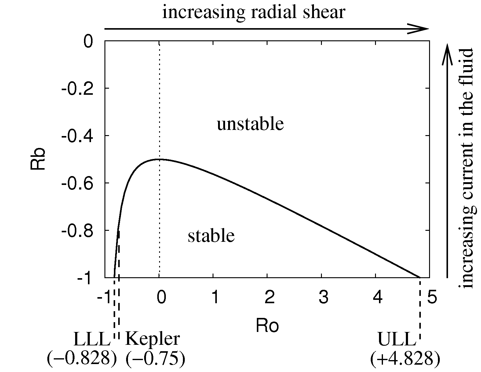
Figure 1: Stability chart in the ${\rm Ro}-{\rm Rb}$ plane, for ${\rm Pm}=0$, ${\rm Ha}$ and ${\rm Re}$ tending to infinity, and optimized values of $\beta$ (for HMRI) or $\alpha$ (for AMRI). The Liu limits LLL and ULL apply only for ${\rm Rb}=-1$, while for ${\rm Rb}>-1$ shallower shear profiles can also be destabilized (including Kepler rotation starting at ${\rm Rb}=0.78125$.). The dotted line separates flows with negative shear (to the left) and positive shear (to the right).

The secular equation (15) has been analyzed in much detail using Bilharz’ stability criterion Kirillov_2013 ; Kirillov_2014 . One of the most important results refers to the limiting stability curve (see Fig. 1) in the ${\rm Ro}-{\rm Rb}$ plane, which obeys the analytical equation

$${\rm Rb}=-\frac{1}{8}\frac{({\rm Ro}+2)^{2}}{{\rm Ro}+1}\;.$$ (18)

The crossing points of this curve with the abscissa (${\rm Rb}=-1$) recover the original result of Liu_2006 , that for ${\rm Pm}=0$, and optimal values of $\beta$, the instability domains lie outside the stratum

$$2-2\sqrt{2}=:{\rm Ro}_{\rm LLL}<{\rm Ro}<{\rm Ro}_{\rm ULL}:=2+2\sqrt{2},$$

where ${\rm Ro}_{\rm LLL}=2(1-\sqrt{2}\approx-0.828$ denotes the lower Liu limit (LLL), as we call it now, and ${\rm Ro}_{\rm ULL}=2(1+\sqrt{2})\approx 4.828$ the upper Liu limit (ULL).

Figure 1 shows that the LLL and ULL are just the endpoints of a quasi-hyperbolic curve. At ${\rm Rb}=-1/2$ the branches for negative shear ${\rm Ro}<0$ and positive shear ${\rm Ro}>0$ meet each other. We find that in the inductionless case ${\rm Pm}=0$, when the Reynolds and Hartmann numbers tend to infinity in a well defined manner Kirillov_2014 and $\beta$ or $n$ are optimized, the maximum achievable critical Rossby number ${\rm Ro}_{\rm extr}$ increases with the increase of ${\rm Rb}$. At ${\rm Rb}\geq-25/32=-0.78125$, ${\rm Ro}_{\rm extr}$ would even exceed the critical value for the Keplerian flow. Therefore, the very possibility for $B_{\phi}(r)$ to depart from the profile $B_{\phi}(r)\propto r^{-1}$ allows us to break the conventional lower Liu limit and extend the inductionless versions of MRI to velocity profiles $\Omega(r)$ as flat as the Keplerian one and even to less steep profiles.

One might ask whether there is any deeper physical sense behind the two Liu limits and the line connecting them. In order to clarify this point, we have investigated in Mama_2016 the non-modal dynamics of HMRI arising from the non-normality of the operator $\bf H$ in Eq. (15). For $\rm Pm\ll 1$ we traced the entire time evolution of the optimal growth of the perturbation energy and demonstrated how the non-modal growth smoothly carries over to the modal behavior at large times. At small and intermediate times, HMRI undergoes a transient amplification. It turned out that the modal growth rate of HMRI displays a very similar dependence on $\rm Ro$ as the maximum non-modal growth of the purely hydrodynamic shear flow. In particular, the optimized non-modal growth rate $G_{m}$ turned out to be identical at the two Liu limits, namely $G_{m}=(1+{\rm Ro})^{sign({\rm Ro})}=5.828$! This indicates a fundamental connection between non-modal dynamics and dissipation- induced modal instabilities, such as HMRI. Despite the latter being magnetically triggered, both rely on hydrodynamic means of amplification, i. e., they extract energy from the background flow mainly by Reynolds stress.

1D and 3D simulations

Actually, the apparently simpler WKB analysis of HMRI, AMRI and TI, as sketched above, was preceded by many detailed 1D and 3D simulations Hollerbach_2005 ; Hollerbach_2010 ; Ruediger_2005 ; Ruediger_2007 . Specifically, the first predictions of HMRI Hollerbach_2005 ; Ruediger_2005 and AMRI Hollerbach_2010 ; Ruediger_2007 were done with 1D codes solving a linear eigenvalue problem for determining the stability thresholds.

Figure  2 shows a recent example for predicting the AMRI experiment at the PROMISE facility (to be discussed below). For the experimentally relevant values ${\rm Pm}=10^{-6}$, ${\rm Re}=3000$, $\mu:=f_{o}/f_{i}=0.26$, and varying $\rm Ha$, the left column shows the normalized growth rate (a), the normalized drift rate (b), and the normalized wave number (c), all obtained with the linear eigenvalue solver Ruediger_2014 . Evidently, the unstable region extends from ${\rm Ha}\approx 80$ to ${\rm Ha}\approx 400$. The right column (d) shows the radial magnetic field component of the AMRI pattern which was computed with the 3D fully non-linear code described in Gellert_2007 .

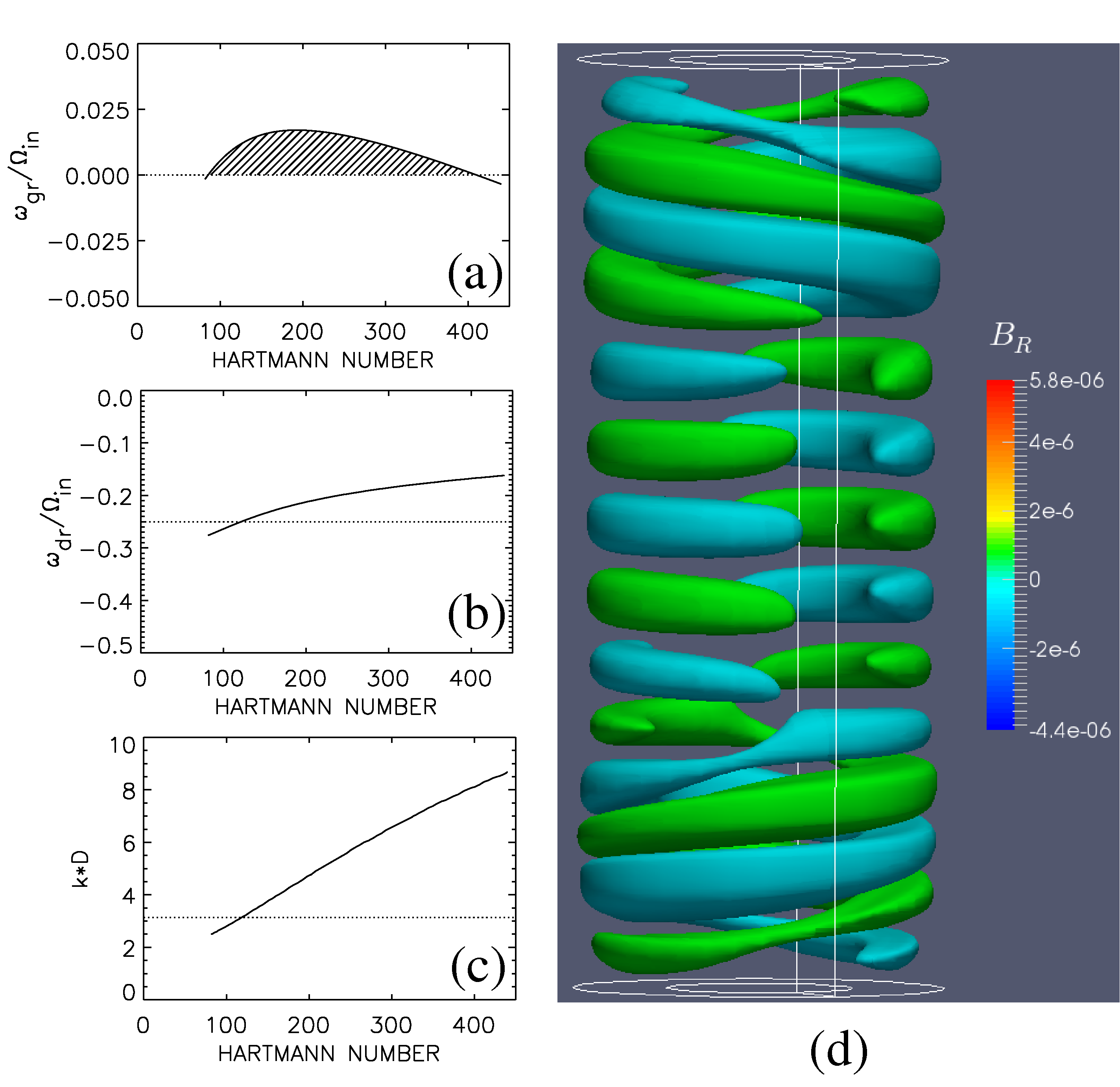
Figure 2: Numerical simulations for the AMRI experiment. Left: Results of a 1D linear eigenvalue solver giving the normalized growth rate (a), the normalized drift frequency (b), and the normalized wave number (c). (d) Radial magnetic field computed with a 3D nonlinear code, at $\rm Re=1500$, $\rm Ha=100$, $\mu=0.26$ and $\rm Pm=10^{-5}$ with split end-plates in units of the applied external field.

More recent numerical results include the proof that Chandrasekhar’s supposedly stable solution Chandra_1956 , in which the Alfvén velocity of the azimuthal field equals the rotation velocity of the background flow, becomes unstable against non-axisymmetric perturbations if at least one of the diffusivities is finite Ruediger_2015 . Another example of such (double-)diffusive instabilities is the magnetic destabilization of flows with positive shear Ruediger_2016 .

Turbulent diffusion

Observations of the present sun with its nearly rigidly rotating core, and of far-developed main-sequence stars, lead to the conclusion that a mechanism must exist that transports angular momentum rather effectively outwards. Since the radiative cores are stably stratified, convection is most probably not relevant here. Furthermore, the sought-after mechanism should enhance the transport of chemicals only mildly, with an effective diffusion coefficient $D_{\rm turb}$ exceeding the molecular viscosity by one or two orders of magnitude Schatzmann_1977 . The authors of Lebreton_1987 considered a relation $D_{\rm turb}={\rm Re}^{*}\nu$ for the diffusion coefficient (after the notation of Schatzman, see Zahn_1990 ) with ${\rm Re}^{*}\simeq 100$. While it has been known for some time that magnetic instability could provide enhanced angular momentum transport (see Spada_2016 ), we show in the following that it also leads to a Schatzman number ${\rm Re}^{*}$ of the correct magnitude.

The numerical model is based on a Taylor-Couette set-up with a current-driven magnetic field that becomes unstable due to the Tayler instability. The whole system rotates differentially with a quasi-Keplerian rotation profile ($\mu=0.354$ for a radius ratio of $r_{i}/r_{o}=0.5$). The most unstable mode is the $m=1$ that grows and saturates. Now the additional diffusion equation (5) is switched on and the enhanced or turbulent diffusion coefficient $D_{\rm turb}$ due to the TI is measured (in units of the molecular diffusion coefficient $D_{\rm mol}$) Paredes_2016 .

The resulting ratio $D_{\rm turb}/D_{\rm mol}$ for a fixed Hartmann number is shown in Fig. 3a. In the slow rotation regime (with a magnetic Mach number ${\rm Mm}={\rm Rm}/{\rm S}<1$), the effective diffusivity hardly changes and is very close to zero. In the fast rotation regime, the ratio $D_{\rm turb}/D_{\rm mol}$ increases monotonically until it reaches a maximum at about ${\rm Mm}\simeq 2$. Finally, for faster rotation (${\rm Mm}>2$), the effective diffusivity decreases rapidly due to the rotational quenching and reaches a rather constant value. Nevertheless, the effective normalized diffusivity always increases with increasing Schmidt numbers so that the Schatzman relation $D_{\rm turb}\propto\nu$ is valid without any influence from the microscopic diffusivity.

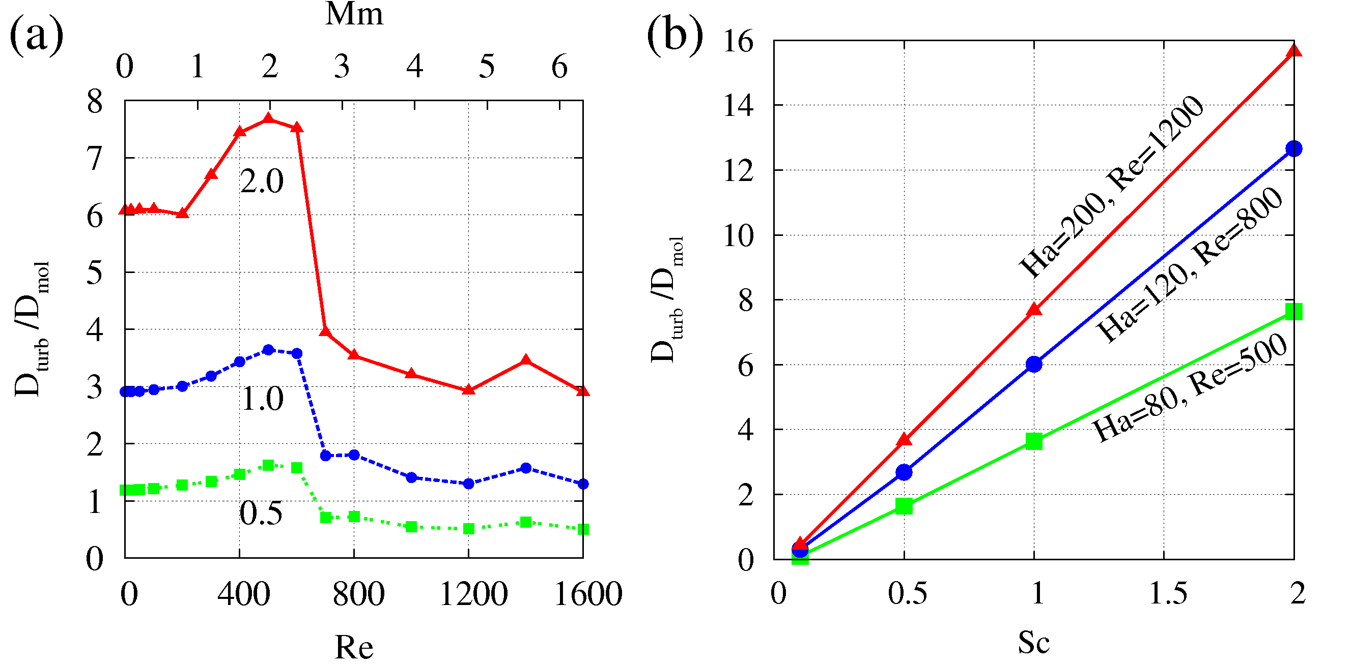
Figure 3: Turbulent contribution to the diffusivity or mixing of TI-unstable flows. (a) Reynolds number dependence of $D_{\rm turb}$ for three values of the Schmidt number ${\rm Sc}=0.1/1/2$ with ${\rm Ha}=80,{\rm Pm}=0.1$. The value ${\rm Mm}=1$ (top horizontal axis) separates the regimes of slow and fast rotation. Note the reduction of $D_{\rm turb}/D_{\rm mol}$ for ${\rm Mm}>2$. (b) Schmidt number dependence with increasing slope or Schatzman ${\rm Re}^{*}$. Always $\mu=0.35$.

Figure  3b shows the normalized diffusivity for fixed Hartmann number as a function of ${\rm Sc}$. For all Reynolds numbers, the induced diffusivities $D_{\rm turb}$ are different from zero, and the ratio $D_{\rm turb}/D_{\rm mol}$ scales linearly with ${\rm Sc}$. The figure only shows the relation for those Reynolds numbers for which the diffusivities reach their maximum at ${\rm Mm}\approx 2$. For ${\rm Sc}\to 0,$ the diffusivity $D_{\rm turb}$ vanishes as well. However, the essential result is the linear relation between $D_{\rm turb}/D_{\rm mol}$ and ${\rm Sc}$ for molecular Schmidt numbers ${\rm Sc}>0.1$. In the notation of Schatzman this means $D_{\rm turb}={\rm Re}^{*}\ \nu$ with the scaling factor ${\rm Re}^{*}$ (which indeed forms some kind of Reynolds number). This linear relation holds for all considered Reynolds and Hartmann numbers.

The scaling or Schatzman factor ${\rm Re}^{*}$ increases with increasing ${\rm Ha}$, while for all three shown parameter sets the magnetic Mach number is nearly the same. We find ${\rm Re}^{*}\sim 4$ for ${\rm Ha}=80$ increasing to ${\rm Re}^{*}\sim 8$ for ${\rm Ha}=200$. A saturation for larger ${\rm Ha}$ is indicated by the results presented in Fig. 3 and would be of the order of 50, which is indeed the right magnitude of the additional diffusion process acting in the sun.

2.2 Experiments on HMRI

Shortly after the theoretical prediction of HMRI Hollerbach_2005 the PROMISE experiment was set-up at HZDR. Its heart is a cylindrical vessel made of copper (Fig. 4). The inner wall extends in radius from 22 to 32 mm; the outer wall extends from 80 to 95 mm. This vessel is filled with the alloy GaInSn, which is a most convenient medium as it is liquid at room temperatures. The physical properties of GaInSn at 25^∘C are: density $\rho=6.36\times 10^{3}$ kg/m³, kinematic viscosity $\nu=3.40\times 10^{-7}$m²/s, electrical conductivity $\sigma=3.27\times 10^{6}$ S/m. The magnetic Prandtl $\rm Pm$ is therefore $1.4\times 10^{-6}$.

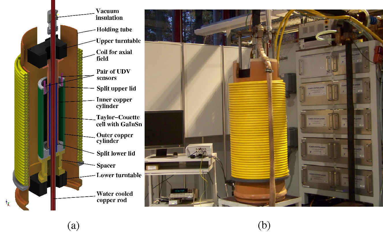
Figure 4: The PROMISE experiment: (a) Schematic sketch of the central Taylor-Couette set-up and the coil for producing the axial field. (b) Photograph of the installation, with the 20 kA power supply visible on the right.

The copper vessel is fixed via a spacer on a precision turntable. Hence, the outer wall of the vessel serves also as the outer cylinder of the Taylor-Couette flow. The inner cylinder of the Tayler-Couette flow is fixed to an upper turntable, and is immersed into the GaInSn from above. It has a thickness of 4 mm, extending from 36 to 40 mm. The actual Taylor-Couette flow then extends between $r_{i}=40$ mm and $r_{o}=80$ mm. In the very first set-up, PROMISE 1 Stefani_2006 ; Stefani_2007 , the upper end-plate was a plexiglass lid fixed to the frame while the bottom was simply part of the copper vessel, and hence rotated with the outer cylinder. There was thus a clear asymmetry in the end-plates, with respect to both their rotation rates and electrical conductivity.

In the second version, PROMISE 2 Stefani_2009 , the lid-configuration was significantly improved by using insulating rings both on top and bottom, and by splitting them at a well defined intermediate radius of 56 mm which had been found in Szklarski_2007 to minimize the Ekman pumping.

With this set-up, HMRI has been comprehensively characterized by varying various parameters and comparing the observed travelling wave structure with numerical predictions. The variations included those of the Reynolds number $\rm Re$, of the ratio $\mu=f_{o}/f_{i}$ of rotation rates, of the Hartmann number $\rm Ha$, and of the ratio $\beta$ of azimuthal to axial field. Figure 5 illustrates a typical result for the latter variation. Fixing $f_{i}=0.06$ Hz, $\mu=0.26$, $I_{\rm coil}=76$ A, we varied the axial current between 0 and 8.2 kA. We observe a travelling HMRI wave only above 4 kA (Fig. 5a). The comparison with numerical predictions is shown in Fig. 5b. The two triangles indicate the numerically determined thresholds for the convective and the absolute instability. The experimental curve suggests that the observed instability is indeed a global one.

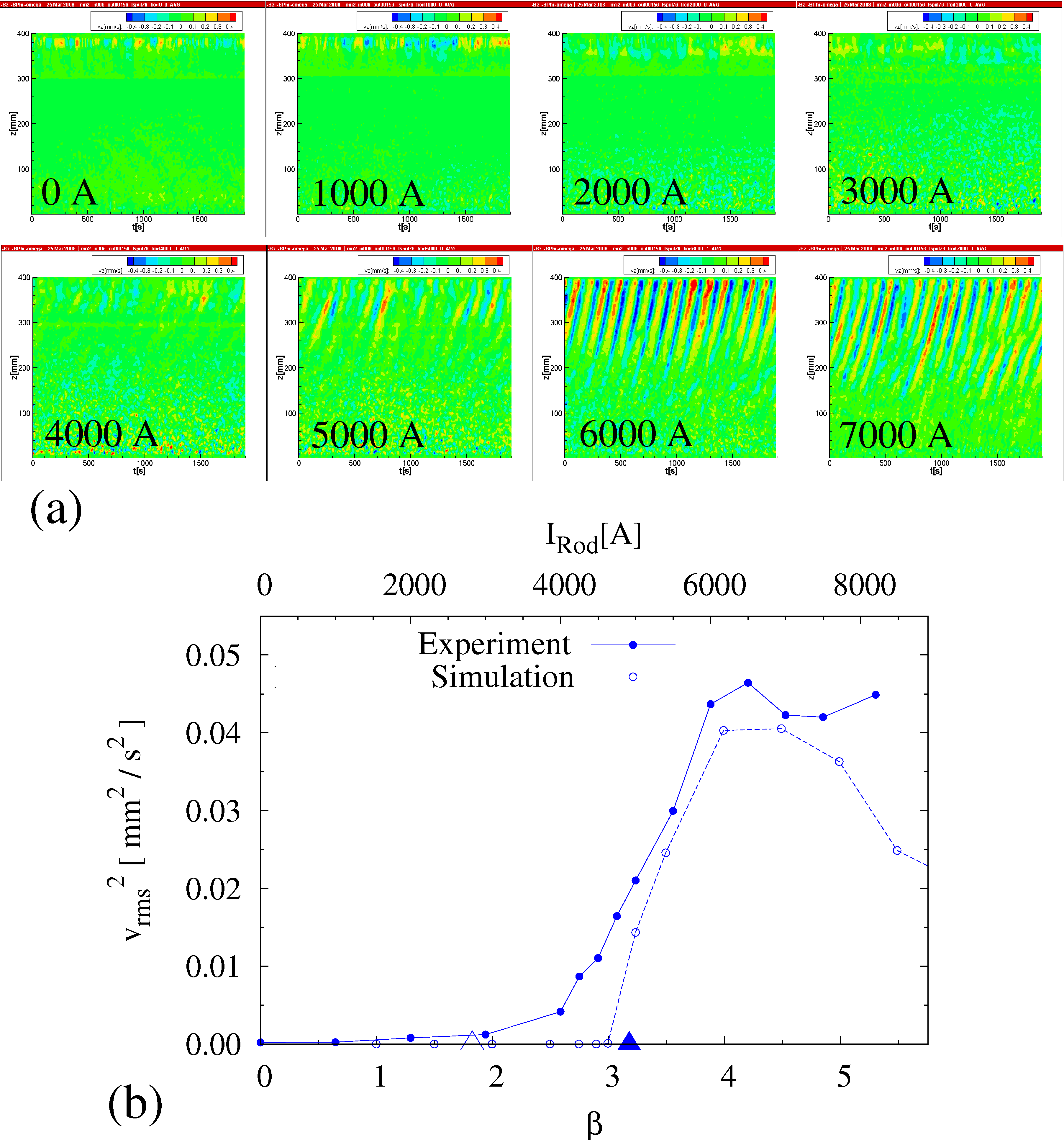
Figure 5: Results of the PROMISE experiment, when varying the axial current. The fixed parameters are $f_{i}=0.06$ Hz, $f_{o}=0.0156$ Hz, resulting in $\rm Re=1775$ and $\mu=0.26$, $I_{\rm coil}=76$ A, giving $\rm Ha=12$. (a) Measured UDV signals in dependence on time (abscissa) and vertical position (ordinate axis), for 8 different axial currents $I_{\rm rod}$. (b) Rms of the perturbation of the axial velocity at the UDV sensor position, in dependence on $I_{\rm rod}$. The dashed line shows the numerical predictions, the full line shows the experimental results. The triangles give the numerical prediction for the onset of the convective instability (empty triangle) and the absolute instability (full triangle).

2.3 Experiments on AMRI

What happens in the PROMISE experiment when we switch off the axial magnetic field? The theoretical predictions for this case have been given in Hollerbach_2010 . The axisymmetric ($m=0$) HMRI is then replaced by the non-axisymmetric ($m=1$) AMRI. At the same time, the threshold of the Hartmann number increases to 80 which requires a central current of approximately 10 kA Seilmayer_2014 .

In order to explore that parameter region, the power supply for the central rod, restricted previously to 8 kA, was replaced by a new one which is able to deliver 20 kA. Connected with this enhancement of the switching mode power supply, significant effort had to be spent on various issues of electromagnetic interference Seilmayer_2016 , before the (initially extremely noisy) UDV data could be utilized for characterizing the AMRI.

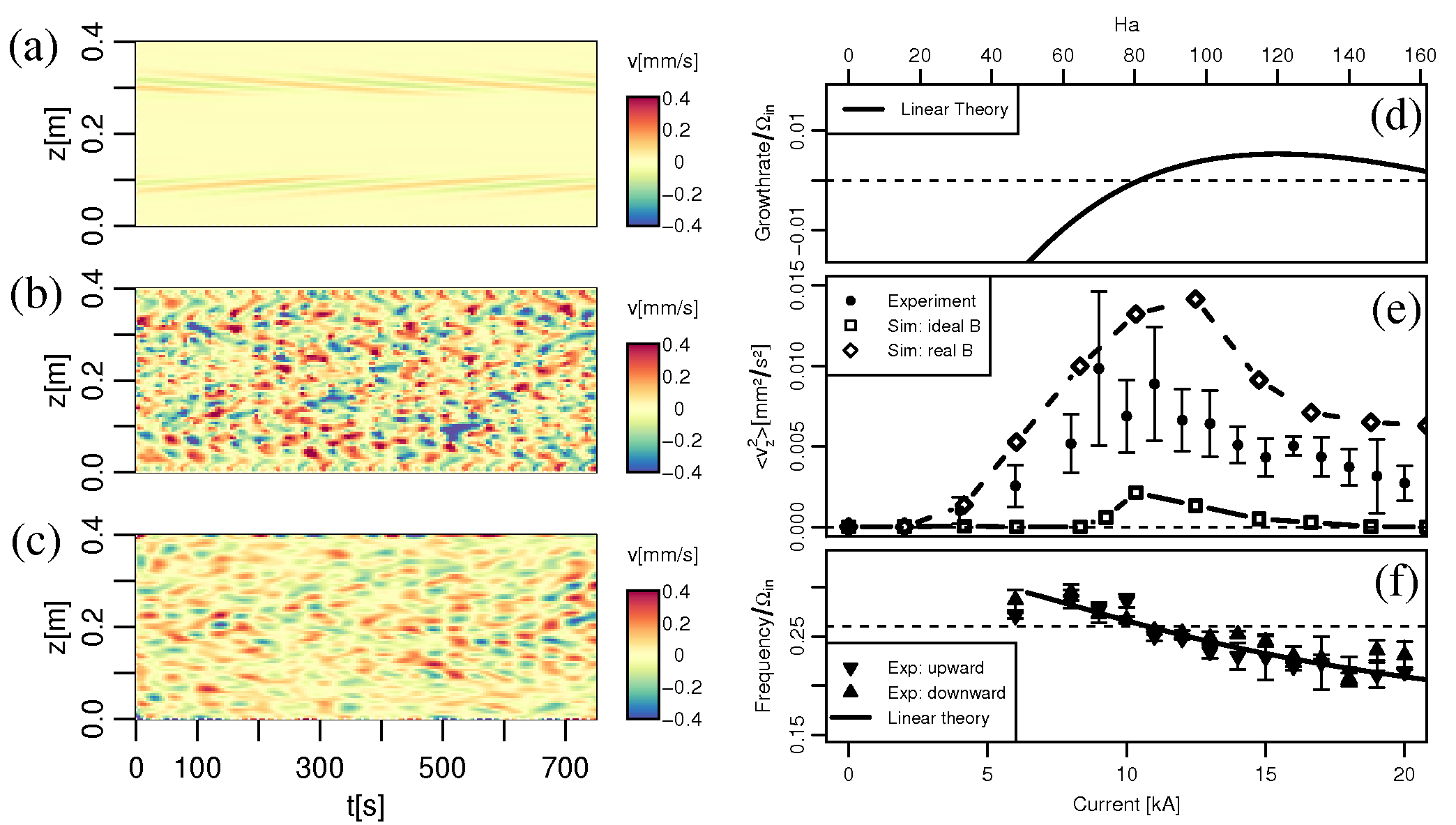
Figure 6: Results of the AMRI experiment. Left: Velocity perturbation $v_{z}(m=1,z,t)$ for $\mu=0.26$, $\rm Re=1480$, and ${\rm Ha}=124$. (a) Simulation for ideal axisymmetric field. (b) Simulation for realistic field. (c) Experimental results. Right: Dependence of various quantities on $\rm Ha$: (d) Numerically determined growth rate. (e) Mean squared velocity perturbation. (f) Angular drift frequency. In the frequency plot, “upward” and “downward” refer to the travel direction of the AMRI wave. After Seilmayer_2014 .

Another problem that became evident when analyzing the data was the factual slight asymmetry of the allegedly axisymmetric field which results from the one-sided wiring of the central vertical current (Fig. 4b). While the observable AMRI structure was originally expected to be similar to that shown in Fig. 2d, a more sophisticated numerical analysis revealed the specific effect of the slight symmetry breaking. This is illustrated in Fig. 6a which shows the spatio-temporal structure of the AMRI wave as it would be expected for a perfectly symmetric, purely azimuthal magnetic field produced by infinitely long wire at the central axis. The parameters for this simulations are $\rm Re=1479$, $\rm Ha=124$. What comes out here is a very regular ”butterfly” diagram of downward and upward traveling waves which are concentrated in the upper and lower half of the cylinder, respectively. While in an infinitely long cylinder upward and downward travelling waves should be equally likely, it is the breaking of axial symmetry due to the effect of the end-caps that induces a preference for upward or downward travelling waves in the two halves of the vessel.

Interestingly, the effect of this first symmetry breaking in axial direction (due to the end-caps) is neutralized by the second symmetry breaking in azimuthal direction (due to the one sided wiring). As a result, the upward and downward travelling waves interpenetrate each other in the two halves of the cylinder. This effect has been revealed both in a numerical simulation which respects the correct geometry (Fig. 6b), as well as in the experiment (Fig. 6c). In Fig. 6d-e we summarize the results for varying Hartmann numbers, including the simulated growth rate (d), the measured and predicted rms of the velocity perturbation (e), and the measured and simulated drift frequencies (f).

While the observed and numerically confirmed effects of the double symmetry breaking on the AMRI are interesting in their own right, we have decided to improve the experiment in such a way that the azimuthal symmetry breaking is largely avoided. This is accomplished by a new system of wiring of the central current, comprising now a ”pentagon” of 5 back-wires situated around the experiment. First experiments with this set-up show encouraging results. Any details, in particular on the transitions between AMRI and HMRI when cranking up the axial magnetic field, are left for future publications.

2.4 Experiments on TI

Imagine the central current used in the AMRI experiment to be complemented, or completely replaced, by a parallel current guided through the fluid column. This current provides a further energy source for instabilities that adds to any prevailing differential rotation. In the limiting case of vanishing differential rotation, the purely current-driven, kink-type Tayler instability (TI) will arrive for sufficiently large currents.

In principle, this effect has been known for a long time in plasma physics, where the (compressible and non-dissipative) counterpart of TI is better known as the kink instability in a $z$-pinch Bergerson_2006 . In astrophysics, TI has been discussed as a possible ingredient of an alternative, nonlinear stellar dynamo mechanism (Tayler-Spruit dynamo Spruit_2002 ; Stefani_2016a ), as a mechanism for generating helicity Gellert_2008 , and as a possible source of helical structures in galactic jets and outflows Moll_2008 . A particular, though non-astrophysical, motivation to study the TI in liquid metals arises from the growing interest in large-scale liquid metal batteries as supposedly cheap storages for renewable energies. Such a battery would consist of a self-assembling stratification of a heavy liquid half-metal (e. g. Bi, Sb) at the bottom, an appropriate molten salt as electrolyte in the middle, and a light alkaline or earth alkaline metal (e. g. Na, Mg) at the top. While small versions of this battery have already been tested Kim_2012 , for larger versions the occurrence of TI could represent a serious problem for the integrity of the stratification Stefani_2011 ; Stefani_2016 ; Weber_2013 ; Weber_2014 ; Weber_2015 .

For liquid metals, TI is expected to set in at an electrical current in the order of kA. The precise value is a function of various material parameters, since for viscous and resistive fluids the TI is known Montgomery_1993 ; Ruediger_2011 ; Spies_1988 to depend effectively on the Hartmann number ${\rm Ha}=B_{\varphi}(R)R(\sigma/(\rho\nu)^{1/2}$, where $R$ is the radius of the column.

Here, we summarize experimental results Seilmayer_2012 that confirm the numerically determined growth rates of TI Ruediger_2011 ; Stefani_2011 as well as the corresponding prediction that the critical current increases monotonically with the radius of an inner cylinder.

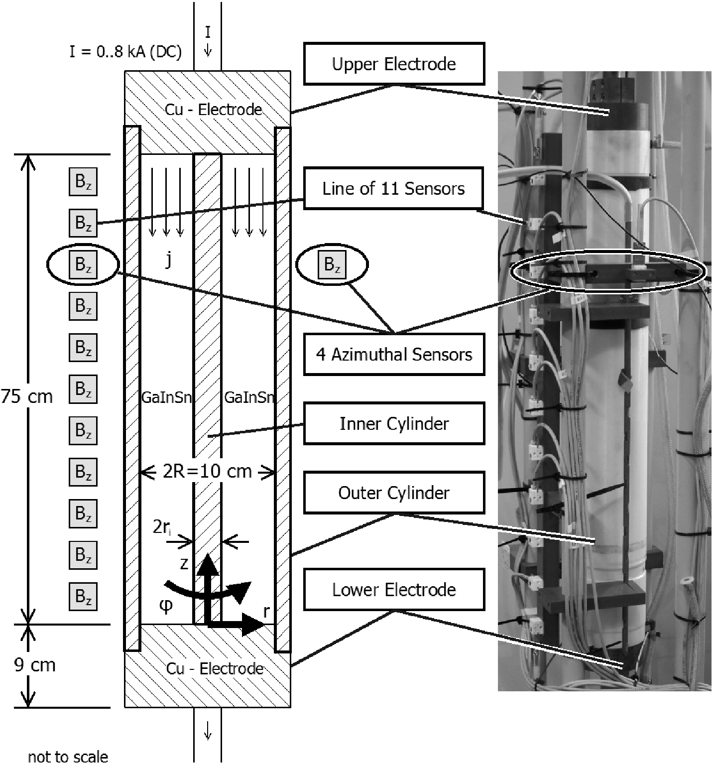
Figure 7: Set-up of the TI-experiment. Left: Scheme with liquid metal column and fluxgate sensors positioned along the vertical axis and the azimuth. Right: Photograph of the central part of the experiment.

The central part of our TI experiment (Fig. 7) is an insulating cylinder of length 75 cm and inner diameter 10 cm, filled again with the eutectic alloy GaInSn. At the top and bottom, the liquid metal column is contacted by two massive copper electrodes of height 9 cm which are connected by water cooled copper tubes to a DC power supply that is able to provide electrical currents of up to 8 kA. By intensively rubbing the GaInSn into the copper, we have provided a good wetting making the electrical contact as homogeneous as possible.

For the identification of TI we exclusively relied on the signals of 14 external fluxgate sensors that measure the vertical component $B_{z}$ of the magnetic field. Eleven of these sensors were aligned along the vertical axis (with a spacing of 7.5 cm), while the remaining three sensors were positioned along the azimuth in the upper part, approximately at 15 cm from the top electrode. The distance of the sensors from the outer rim of the liquid metal column was 7.5 cm. This rather large value, which is certainly not ideal to identify small wavelength perturbations, has been chosen in order to prevent saturation of the fluxgate sensors in the strong azimuthal field of the axial current.

One of the main goal of the experiment was to study the influence of the electric current through the fluid on the growth rate and on the amplitude of the magnetic field perturbations. This was done without any insert, as well as for two different radii of an inner non-conducting cylinder, $r_{i}$=6 mm and 12.5 mm, for which we expect a monotonic increase of the critical current with the radius.

In Fig. 8 we compile the dependence of the growth rate of the TI on the radius of the inner cylinder and on the current through the fluid, and compare them with the numerically determined growth rates Ruediger_2011 for the mode with optimum wavelength (appr. 13 cm). Despite some scatter of the data, we observe a quite reasonable agreement with the numerical predictions.

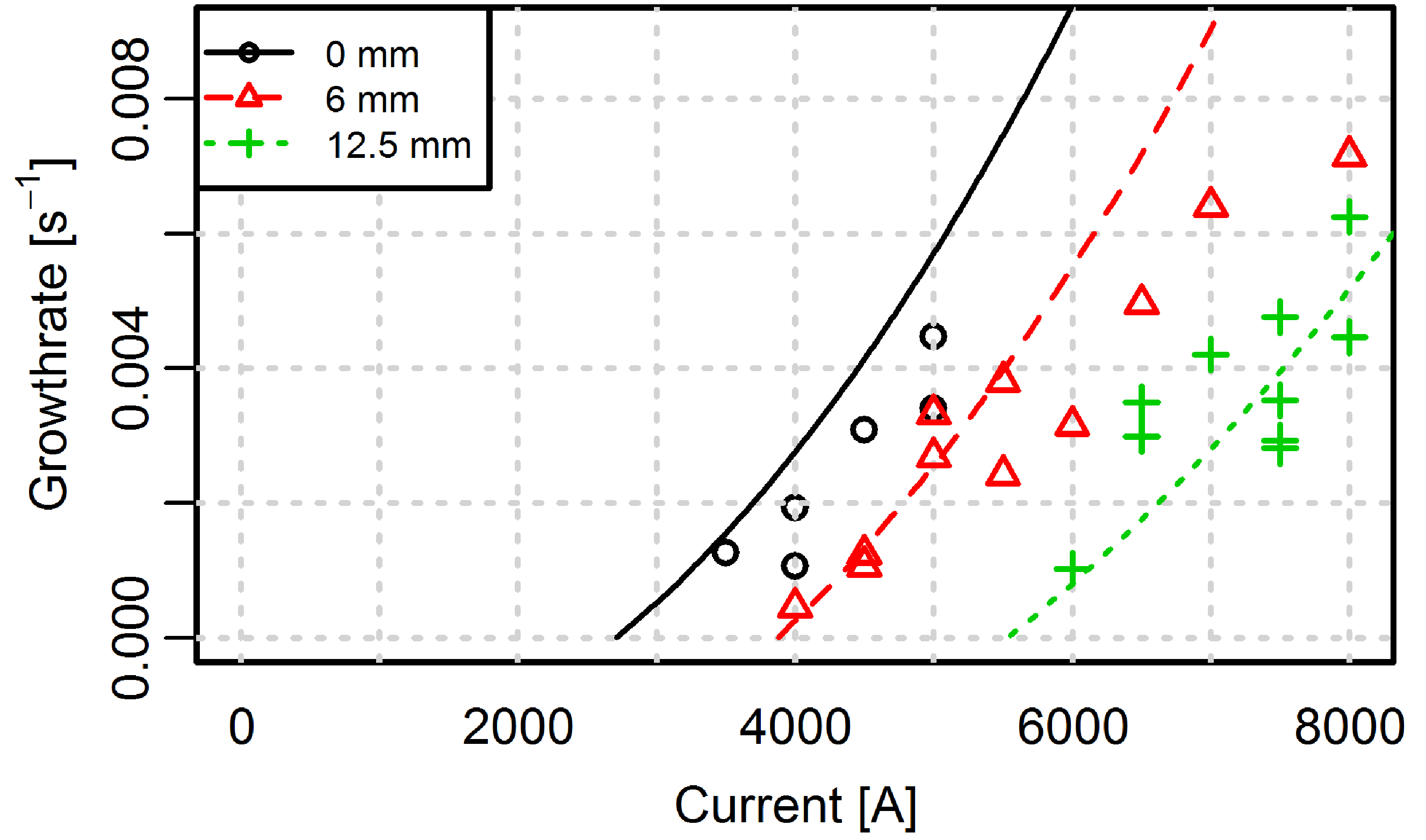
Figure 8: Growth rates of the TI in dependence on the current for three different radii (0, 6, and 12.5 mm) of a central insulating cylinder. The lines give the numerical results, the symbols show the values inferred from the experiment. After Seilmayer_2012 .

We have to admit that the realization and the data analysis of the TI experiment was significantly harder than originally envisioned. The main reason is the indirect identification of the TI by the fluxgate sensors along the height of the column and the azimuth. The very weak induced magnetic fields, the slightly under-critical number of sensors, but also the Joule heating due to the high current densities were main obstacles for a clear identification of the TI.

We note that some later experiments using Ultrasonic Doppler Velocimetry (UDV) in order to measure directly the axial velocity component along the $z$-axis did not really solve the problems Starace_2015 . Actually, they even lead to strong electro-vortex flows driven by the inhomogeneous current distribution at the sensor positions which spoiled significantly the previous TI results obtained with a more homogeneous interface between fluid and copper electrodes.

3 Instabilities in spherical geometry

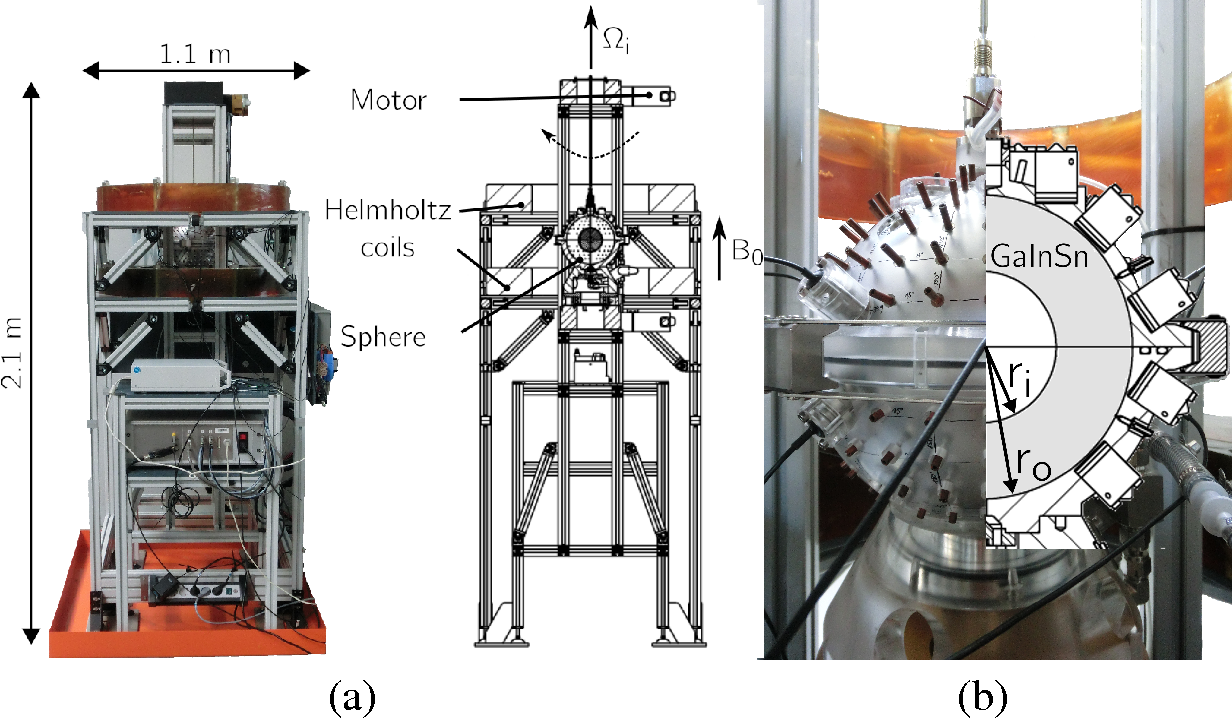
Figure 9: The HEDGEHOG experiment: (a) Photograph and drawing of the facility. (b) Zoom on the spherical Couette module, showing the mountings for the UDV probes and the copper electrodes for electric potential measurements. $r_{i}=4.5$ cm, $r_{o}=9$ cm.

The terminus spherical Couette flow refers to the fluid motion between two differentially rotating spherical shells. If the liquid is electrically conducting and exposed to an external magnetic field, the set-up is sometimes called magnetized spherical Couette flow (MSCF). For resting outer cylinder, the system is completely defined by three dimensionless parameters Ruediger_2013 : the Reynolds number ${\rm Re}=\Omega_{i}r_{i}^{2}/\nu$ as a measure of the rotation (with angular velocity $\Omega_{i}$ of the inner sphere with radius $r_{i}$), the Hartmann number ${\rm{Ha}}=B_{0}r_{i}\sqrt{\sigma/\rho\nu}$ with $B_{0}$ denoting the strength of the applied axial magnetic field, and the geometric aspect ratio $\eta=r_{i}/r_{o}$ with the outer sphere radius $r_{o}$.

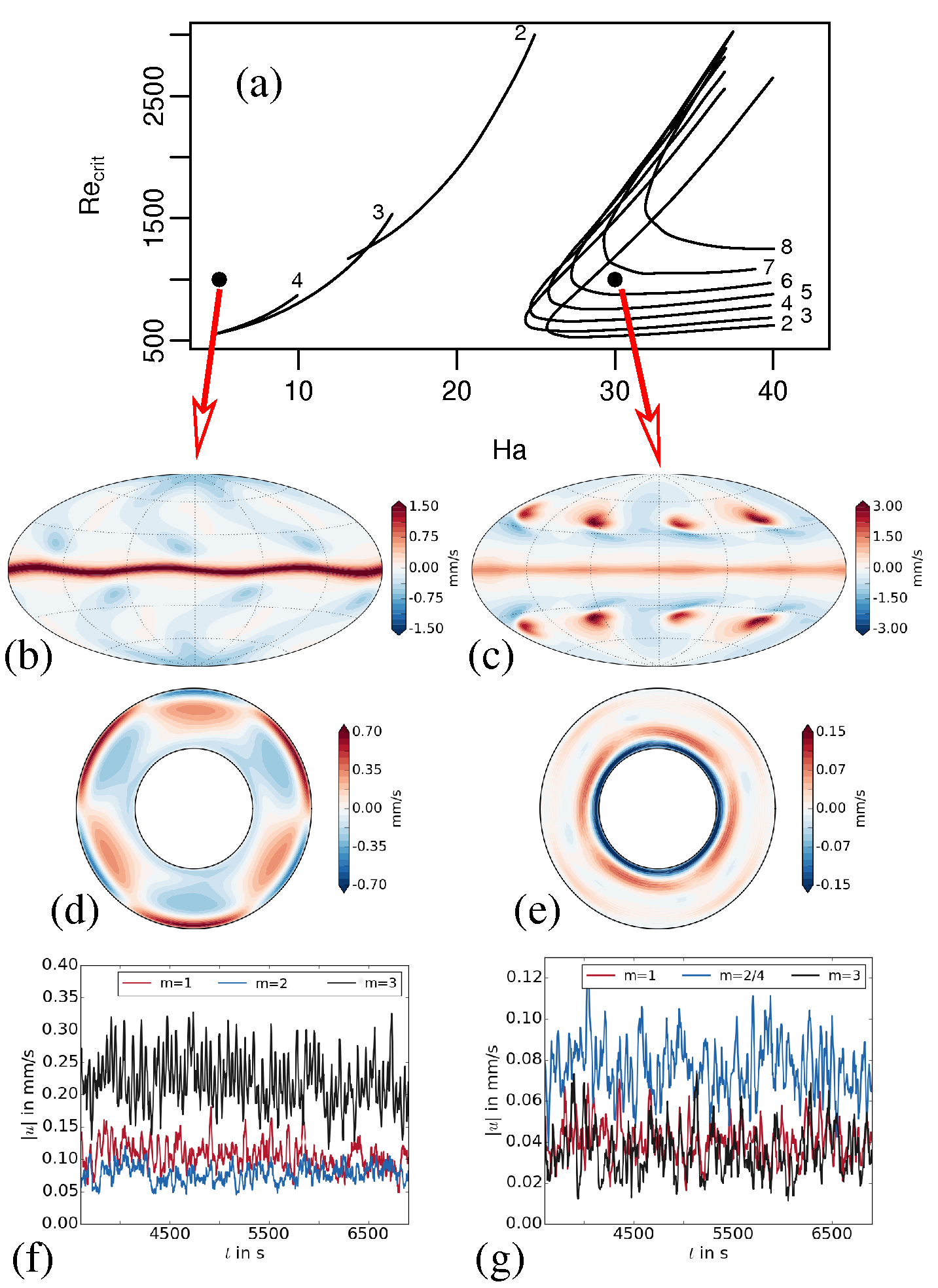
Figure 10: Numerical simulations and experimental results of the HEDGEHOG experiment. (a) Boundaries of instabilities in dependence on $\rm Ha$ and $\rm Re$, reproduced from Travnikov_2011 . Lower left: Jet instability at $\rm Rm=1000$ and $\rm Ha=5$. (b) Meridional view of the simulated radial velocity component at $r=0.85r_{o}$, showing the anti-symmetric character with respect to the equator. (d) Polar view of the meridional velocity component at $\theta=\pi/2$, showing an $m=3$ azimuthal dependence. (f) Azimuthal Fourier components of the UDV measured velocity taken at a depth of 25 mm, showing the expected dominance of the $m=3$ mode. Lower right: Return flow instability at $\rm Rm=1000$ and $\rm Ha=30$. (c) Meridional view of the simulated radial velocity component at $r=0.6r_{o}$, showing the symmetric character with respect to the equator. (e) Polar view of the meridional velocity component at $\theta=\pi/2$, showing an $m=4$ azimuthal dependence. (g) Azimuthal Fourier components of the UDV measured velocity taken at a depth of 36 mm, showing the expected dominance of the $m=4$ mode.

Besides its paradigmatic character, the MSCF gained new attention in the astrophysical community as Sisan et al. Sisan_2004 had claimed the observation of the MRI on the background of a fully turbulent flow. Later, however, Hollerbach Hollerbach_2009 and Gissinger et al. Gissinger_2011 interpreted the observed fluctuations just as turbulent analogues of various well-known MSCF instabilities.

In order to clarify this point, the new apparatus HEDGEHOG (Hydromagnetic Experiment with Differentially Gyrating sphEres HOlding GaInSn) has been installed at HZDR (see Fig. 9). In contrast to Sisan_2004 , HEDGEHOG works in a quasi-laminar regime for which numerical reference data is available for the two particular aspect ratios $\eta=0.35$ Hollerbach_2009 and $\eta=0.5$ Travnikov_2011 .

3.1 Numerical simulations

The experiment has been numerically simulated by two different codes. One is the code described in Hollerbach_2000 which solves for a flow, driven by the rotating inner sphere, according to the incompressible Navier-Stokes Equation including a Lorentz force term. The steady states of the full three-dimensional calculation have the practical use of guiding diagnostic design and expectations for the low $\rm Re$ case. They also demonstrate a saturation mechanism for the instabilities Kaplan_2014 . Complementary to that code, we have also used the MagIC code Wicht_2014 , which has a long and very successful record of simulating dynamos in spherical geometry.

Figure 10 shows the stability boundaries and illustrates two typical instabilities, for a MSCF with aspect ratio $\eta=0.5$. First, Fig. 10a shows the boundaries for the different types of instability in dependence on $\rm Ha$. Actually, the lines have been replotted from Travnikov_2011 , although large parts of the diagram were reproduced by Hollerbach’s code. The two full circles represent the two distinct types of instability which are separated by a region of stability. Their spatial character, as simulated by the MagIC code, is illustrated in Fig. 10b-e.

At low ${\rm Ha}=5$, the instability arises in the equatorial jet, see Fig. 10b,d. It is anti-symmetric with respect to the equator, and characterized by an $m=3$ azimuthal dependence. At higher ${\rm Ha}=30$, the instability arises along the Shercliff layer, see Fig. 10c,e, it is symmetric with respect to the equator, and has an $m=4$ azimuthal dependence.

3.2 The HEDGEHOG experiment

HEDGEHOG (see Fig. 9) consists of one of two optional inner spheres ($r_{i}=3$ cm or 4.5 cm) held in the center of an outer sphere ($r_{o}=9$ cm). The outer sphere is a Polymethyl Methacetate (PMMA) acrylic with 30 cylindrical holders for ultrasonic Doppler velocimetry (UDV), and 168 copper electrodes for electric potential measurement.

The space between the spheres is filled with GaInSn. Because of the high density of this medium, each optional inner sphere holds a lead weight to counter the buoyancy force. The axial magnetic field is provided by a pair of copper electromagnets with central radii of 30 cm, with a vertical gap of 31 cm between them (a near Helmholtz configuration). The spheres can be driven with a minimum rotation frequency $f_{i}=0.02$ Hz by 90 W electromotors.

The data presented here is based on the velocity acquired from six equally spaced UDV sensors on the northern hemisphere (NH), and from one UDV sensor on the southern hemisphere (SH). This sensor configuration allows to identify (roughly) the azimuthal dependence of the modes and their symmetry properties with respect to the equator.

For low $\rm Ha$ the UDV sensors show an outward directed velocity around the depth of the equatorial plane. This is the radial jet whose instability is known from the purely hydrodynamic case Hollerbach_2006 . Increasing $\rm Ha$ further, the jet is suppressed and a growing area with zero velocity values comes up. At still higher $\rm Ha$ new velocity fluctuations occur at greater depth of the UDV beam.

Using 6 sensor data in azimuthal direction, according to the Nyquist-Shannon criterion a maximum wave number $m=3$ can be resolved by Fourier transform. Further to this, the frequency of the equatorially symmetric and anti-symmetric velocity parts can be inferred from spectrograms. Using the data from the facing NH and SH UDV pair, the equatorial symmetric part is computed as $(u_{\rm{NH}}+u_{\rm{SH}})/2$, and the anti-symmetric part as $(u_{\rm{NH}}-u_{\rm{SH}})/2$. Figure 10f shows the Fourier transform of the anti-symmetric part taken at a depth of 25 mm For this low $\rm Ha=5$ we clearly recognize a dominating azimuthal $m=3$ mode, also with the numerically predicted frequency (not shown here).

At $\rm Ha=30$ the instability is distinctly shifted towards the inner sphere and acquires an equatorially symmetric character, which indicates the onset of the return flow instability. Figure 10g shows the Fourier transform of the symmetric part taken at a depth of 36 mm. We clearly recognize a dominating azimuthal $m=4$ mode, also with the numerically predicted frequency.

The wave number and frequency observations at the chosen $\rm Re=1000$ and increasing values of $\rm Ha$ are in good agreement with numerical predictions. In future, electric potential measurements will help to resolve the remaining ambiguities with respect to the azimuthal wave number of the observed modes.

4 Conclusions and Outlook

Despite the significant theoretical and experimental achievements on the various inductionless forms of shear or current-driven instabilities, the unambiguous laboratory proof of SMRI is still elusive. In the following we will sketch our plans for a large-scale liquid sodium experiment which is supposed to allow for studying the transition between the inductionless versions such as HMRI and AMRI to SMRI.

Further to this, we will also delineate the prospects for laboratory studies of instabilities of rotating flows with positive shear.

4.1 The large MRI/TI experiment

The DREsden Sodium facility for DYNamo and thermohydraulic studies (DRESDYN) is intended as a platform both for large-scale experiments related to geo- and astrophysics as well as for experiments related to thermohydraulic and safety aspects of liquid metal batteries and liquid metal fast reactors. The most ambitious project in the framework of DRESDYN is a homogeneous hydromagnetic dynamo driven solely by precession Stefani_2012 ; Stefani_2015 .

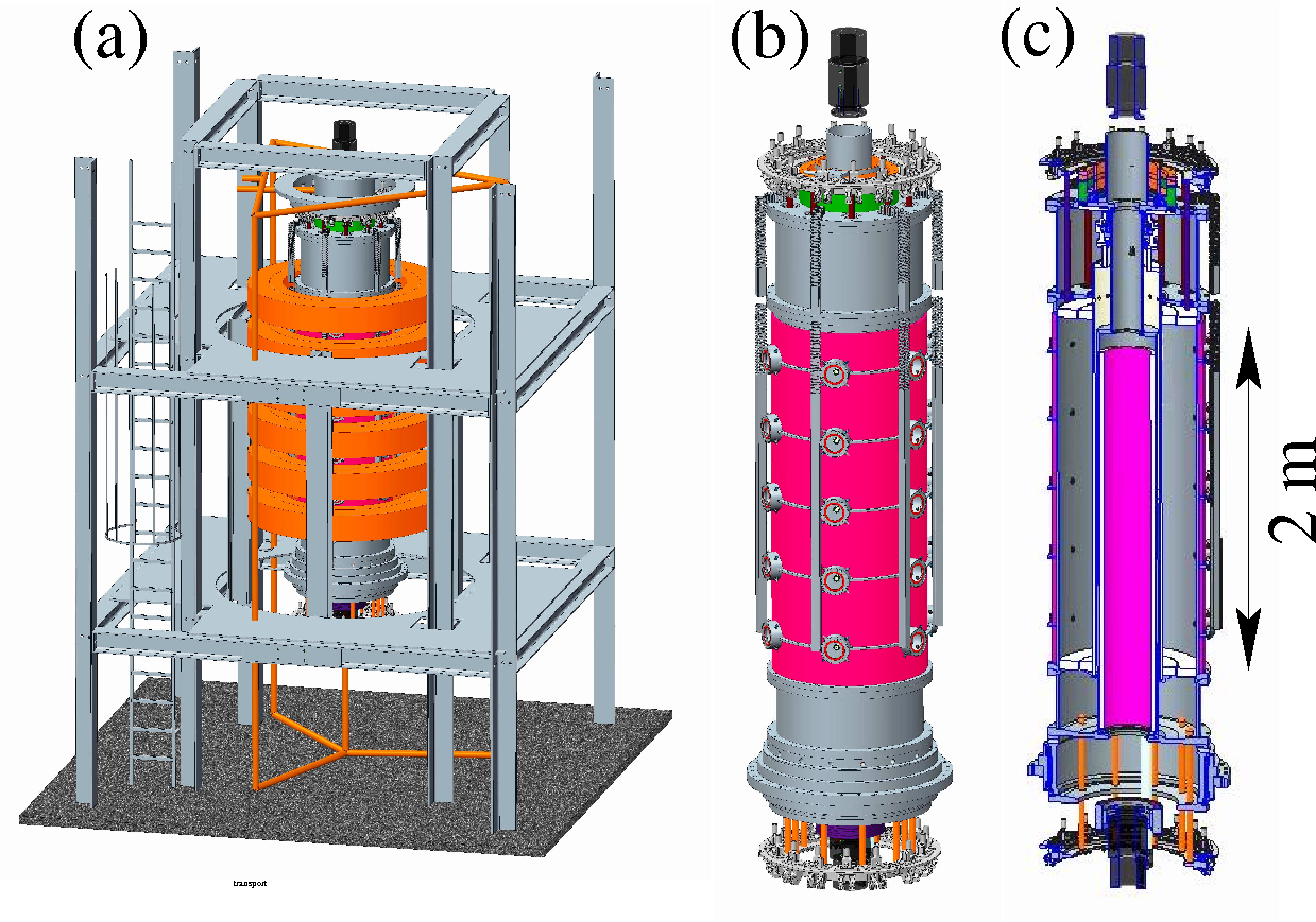
Figure 11: Drawings of the combined MRI/TI experiment as planned in the framework of the DRESDYN project. (a) Total view. (b) Central module from outside. (c) Central module from inside.

A second large-scale experiment relevant to geo- and astrophysics will investigate combinations of different versions of the MRI with the current-driven TI (see Fig. 11). Basically, the set-up is designed as a Taylor-Couette experiment with 2 m height, an inner radius $r_{i}=20$ cm and an outer radius $r_{o}=40$ cm. Rotating the inner cylinder at up to 20 Hz, we plan to reach ${\rm Rm}\sim 40$, while the maximum axial magnetic field $B_{z}=120$ mT will correspond to a Lundquist number $S:={\rm Pm}^{1/2}{\rm Ha}\sim 8$. Both values are about twice their respective critical values for SMRI as they were derived in Ruediger_2003 .

Below those critical values, we plan to investigate how the helical version of MRI approaches the limit of SMRI Hollerbach_2005 . To this end, we will use a strong central current, as it was already done in the PROMISE experiment Seilmayer_2014 ; Stefani_2009 . This insulated central current can be supplemented by another axial current guided through the (rotating) liquid sodium, which will then allow to investigate arbitrary combinations of MRI and TI. As discussed in Sec. 2, theoretical studies Kirillov_2013 ; Kirillov_2014 have shown that even a slight addition of current through the liquid would extend the range of application of the helical and azimuthal MRI to Keplerian flow profiles.

4.2 Positive shear instabilities

The last remarks refer to flows with positive ${\rm Ro}$, i. e. flows whose angular velocity (not only the angular momentum) is increasing outward. From the purely hydrodynamic point of view, such flows are linearly stable (while non-linear instabilities were actually observed in experiments Tsukahara_2010 ). Flows with positive ${\rm Ro}$ are indeed relevant for the equator-near strip (approximately between $\pm 30^{\circ}$) of the solar tachocline Parfrey_2007 , which is, interestingly, also the region of sunspot activity Charbonneau_2010 .

As discussed in Sec. 2, a first hint on a magnetic destabilization of flows with ${\rm Ro}>{\rm Ro}_{\rm ULL}$ was given in the paper Liu_2006 for the case of a helical magnetic field. For a purely azimuthal field, a similar effect was found both in the framework of WKB approximation Stefani_2015b as well as by a 1D modal stability analysis Ruediger_2016 .

What are the prospects for an experiment that could show a magnetic destabilization of positive shear flows? The WKB analysis in Stefani_2015 has revealed the need for a rather narrow gap flow which necessarily leads to comparable high axial currents. For a prospective Taylor-Couette experiment with Na with an outer diameter of $r_{o}=0.25$ m, and choosing ${\eta}=0.85$, those values would be ${\rm{Re}}=1898$, ${\rm{Ha}}=892$ which amounts to physical values of $f_{o}=0.022$ Hz, and $B_{\phi}(r_{i})=77$ mT, requiring a central current of 82 kA !

The 1D simulations of Ruediger_2016 predicted more optimistic values in the order of 30 kA, if the radial boundaries were considered as ideally conducting. It remains to be shown by careful numerical studies what are the real critical currents for an optimized laboratory implementation when realistic conductivity ratios between the liquid (sodium) and the wall material (copper) are taken into account.

- (1) Adams, M.M., Stone, D.R., Zimmerman, D.S., Lathrop, D.P.: Liquid sodium models of the Earth’s core. Prog. Earth Planet. Sci. 29, 1-18 (2015).
- (2) Balbus, S.A.: Enhanced angular momentum transport in accretion disks. Ann. Rev. Astron. Astrophys. 41, 555-597 (2003)
- (3) Benzi, R., Pinton, J.-F.: Magnetic Reversals in a Simple Model of Magnetohydrodynamics. Phys. Rev. Lett. 105, 024501 (2010)
- (4) Bergerson, W.F., Hannum, D.A., Hegna, C.C., Kendrick, R.D., Sarff, J.S., Forest, C.B.: Onset and saturation of the kink instability in a current-carrying line-tied plasma. Phys. Rev. Lett. 96, 015004 (2006).
- (5) Berhanu, M. et al.: Dynamo regimes and transitions in the VKS experiment. Eur. Phys. J. B 77, 459–468 (2010)
- (6) Chandrasekhar, S.: On the stabiluty of the simplest soluation of the equations of hydromagnetics. P. Natl. Acad. Sci. USA 42, 273-276 (1956)
- (7) Charbonneau, P.: Dynamo models of the solar cycle. Liv. Rev. Sol. Phys. 7, 3 (2010)
- (8) Cooper, C.M. et al.: The Madison plasma dynamo experiment: A facility for studying laboratory plasma astrophysics. Phys. Plasmas 21, 013505 (2014)
- (9) Dormy, E.: Strong-field spherical dynamos. J. Fluid Mech. 789, 500-513 (2016)
- (10) Gailitis, A., Lielausis, O., Dement’ev, S., Platacis, E., Cifersons, A., Gerbeth, G., Gundrum, T., Stefani, F., Christen, M., Hänel, H., Will, G.: Detection of a flow induced magnetic field eigenmode in the Riga dynamo facility. Phys. Rev. Lett. 84, 4365–4369 (2000)
- (11) Gailitis, A., Lielausis, O., PLatacis, E., Gerbeth, G., Stefani, F.: Laboratory experiments on hydromagnetic dynamos, Rev. Mod. Phys. 74, 973–990 (2002)
- (12) Gellert, M., Rüdiger, G., Fournier, A.: Energy distribution in nonaxisymmetric magnetic Taylor-Couette flow. Astron. Nachr. 328, 1162-1165 (2007)
- (13) Gellert, M., Rüdiger, G., Elstner, D.: Helicity generation and alpha-effect by Tayler instability with z-dependent differential rotation. Astron. Astrophys. 479, L33–L36 (2008)
- (14) Giesecke, A., Stefani, F., Gerbeth, G.: Role of soft-iron impellers on the mode selection in the von-Karman-sodium dynamo experiment. Phys. Rev. Lett. 104, 044503 (2010)
- (15) Giesecke, A., Nore, C., Stefani, F., Gerbeth, G., Léorat, J., Herreman, W., F., Guermond, J.-L.: Influence of high-permeability discs in an axisymmetric model of the Cadarache dynamo experiment. New. J. Phys. 14, 053005 (2012)
- (16) Gissinger, C., Ji, H., Goodman, J.: Instabilities in magnetized spherical Couette flow. Phys. Rev. E 84, 026308 (2011)
- (17) Hollerbach, R.: A spectral solution of the magneto-convection equations in spherical geometry. Int. J. Num. Meth. Fluids 32, 773–797 (2000)
- (18) Hollerbach, R., Rüdiger, G.: New type of magnetorotational instability in cylindrical Taylor-Couette flow. Phys. Rev. Lett. 95, 124501 (2005)
- (19) Hollerbach, R.: Non-axisymmetric instabilities in basic state spherical Couette flow. Fluid. Dyn. Res. 38, 257–273 (2006)
- (20) Hollerbach, R.: Non-axisymmetric instabilities in magnetic spherical Couette flow. Proc. R. Soc. A 465, 2003–2013 (2009).
- (21) Hollerbach, R., Teeluck, V., Rüdiger, G.: Nonaxisymmetric magnetorotational instabilities in cylindrical Taylor-Couette flow. Phys. Rev. Lett. 104, 044502 (2010).
- (22) Jones, C.A.: Planetary magnetic fields and dynamos. Ann. Rev. Fluid Mech. 43, 583–614 (2011)
- (23) Kaplan, E.: Saturation of nonaxisymmetric instabilities of magnetized spherical Couette flow. Phys. Rev. E. 89, 063016 (2014)
- (24) Kim, H. et al.: Liquid metal batteries: past, present, and future. Chem. Rev. 113, 2075–2099 (2013)
- (25) Kirillov, O.N.; Stefani, F.: On the relation of standard and helical magnetorotational instability. Astrophys. J. 712, 52–68 (2010)
- (26) Kirillov, ON.; Stefani, F.: Paradoxes of magnetorotational instability and their geometrical resolution. Phys. Rev. E 84, 036304 (2011)
- (27) Kirillov, O.N., Stefani, F., Fukumoto, Y.: A unifying picture of helical and azimuthal magnetorotational instability, and the universal significance of the Liu limit. Astrophys. J. 756, 83 (2012)
- (28) Kirillov, O.N., Stefani, F.: Extending the range of the inductionless magnetorotational instability. Phys. Rev. Lett. 111, 061103 (2013)
- (29) Kirillov, O.N., Stefani, F., Fukumoto, Y.: Local instabilities in magnetized rotational flows: a short-wavelength approach. J. Fluid Mech. 760, 591–633 (2014)
- (30) Lathrop, D.P., Forest, C.B.: Magnetic dynamos in the lab. Phys. Today 64, 40–45 (2011)
- (31) Lebreton, Y., Maeder, A.: Stellar evolution with turbulent diffusion mixing. VI - The solar model, surface Li-7, and He-3 abundances, solar neutrinos and oscillations. Astron. Astrophys. 175, 99 (1987)
- (32) Liu, W., Goodman, J., Herron, I., Ji, H.: Helical magnetorotational instability in magnetized Taylor-Couette flow. Phys. Rev. E 74, 056302 (2006)
- (33) Liu, W., Goodman, J., Ji, H.: Traveling waves in a magnetized Taylor-Couette flow. Phys. Rev. E 76, 016310 (2007)
- (34) https://github.com/magic-sph/magic.
- (35) Mamatsashvili, G., Stefani, F.: Linking dissipation-induced instabilities with nonmodal growth: the case of helical magnetorotational instability. arXiv:1604.07205
- (36) Moll. R., Spruit, H.C., Obergulinger, M.: Kink instabilities in jets from rotating magnetic fields. Astron. Astrophys. 492, 621–630 (2008)
- (37) Montgomery, D.: Hartmann, Lundquist, and Reynolds: the role of dimensionless numbers in nonlinear magnetofluid behavior. Phys. Rev. E 87, 012108 (2013)
- (38) Mori, N. Schmitt, D., Wicht, J. Ferriz-Mas, A., Mouri, H., Nakamichi, A. Morikawa, M: Domino model for geomagnetic field reversals. Plasma Phys. Control. Fusion 35, 105–113 (1993)
- (39) Nore, C., Quiroz, D.C., Cappanera, L., Guermond, J.L.: Direct numerical simulation of the axial dipolar dynamo in the Von Kármán Sodium experiment. Europhys. Lett. 114, 65002 (2016)
- (40) Nornberg, M.D., Ji, H., Schartman, E., Roach, A., Goodman, J.: Observation of magnetocoriolis waves in a liquid metal Taylor-Couette experiment. Phys. Rev. Lett. 104, 074501 (2010)
- (41) Paredes, A., Gellert, M., Rd̈iger, G.: Mixing of a passive scalar by the instability of a differentially rotating axial pinch. Adtron. Astrophys. 588, A147 (2016)
- (42) K.P. Parfrey, K. Menou: The origin of solar activity in the tachocline: Astrophys. J. Lett. 667, L207 (2007)
- (43) Petitdemange, L., Dormy, E., Balbus, S.A.: Magnetostrophic MRI in the Earth’s outer core. Geophys. Res. Lett. 35, L15305 (2008)
- (44) Petitdemange, L.: Two-dimensional non-linear simulations of the magnetostrophic magnetorotational instability. Geophys. Astrophys. Fluid Dyn. 104, 287–299 (2010)
- (45) Priede, J., Gerbeth, G.: Absolute versus convective helical magnetorotational instability in a Taylor-Couette flow. Phys. Rev. E 79, 046310 (2009)
- (46) Petrelis, F., Fauve, S., Dormy, E., Valet, J.-P.: Simple mechanism for reversals of Earth’s magnetic field. Phys. Rev. Lett. 102, 144503 (2009)
- (47) Reuter, K., Jenko, F., Tilgner, A., Forest, C.B.: Wave-driven dynamo action in spherical magnetohydrodynamic systems. Phys. Rev. E 80, 056304 (2009)
- (48) Roach, A.H., Spence, E.J., Gissinger, C., Edlund, E.M., Sloboda, P., Goodman, J., Ji, H.: Observation of a free-Shercliff-layer instability in cylindrical geometry. Phys. Rev. Lett. 108, 154502 (2012)
- (49) Rüdiger, G., Shalybkov, D.: Linear magnetohydrodynamic Taylor-Couette instability for liquid sodium. Phys. Rev. E 67, 046312 (2003)
- (50) Rüdiger G., Hollerbach R., Schultz M., Shalybkov D.: The stability of MHD Taylor-Couette flow with current-free spiral magnetic fields between conducting cylinders. Astron. Nachr. 326, 409-413 (2005)
- (51) Rüdiger, G., Hollerbach, R., Schultz, M., Elstner, D.: Destabilization of hydrodynamically stable rotation laws by azimuthal magnetic fields. Mon. Not. R. Astron. Soc. 377, 1481–1487 (2007)
- (52) Rüdiger, G., Gellert, M., Schultz, M.: Eddy viscosity and turbulent Schmidt number by kink-type instabilities of toroidal magnetic fields. Mon. Not. R. Astron. Soc. 399, 996–1004 (2009)
- (53) Rüdiger, G., Schultz, M., Gellert, M.: The Tayler instability of toroidal magnetic fields in a columnar gallium experiment. Astron. Nachr. 332, 17-23 (2011)
- (54) Rüdiger, G., Hollerbach, R., Kitchatinov, L.L.: Magnetic processes in astrophysics: theory, simulations, experiments. WILEY-VCH, Weinheim (2013)
- (55) Rüdiger, G., Gellert, M., Schultz, M., Hollerbach, R., Stefani, F.: Astrophysical and experimental implications from the magnetorotational instability of toroidal fields. Mon. Not. R. Astron. Soc. 438, 271-277 (2014)
- (56) Rüdiger, G., Schultz, M., Stefani, F., Mond. M.: Diffusive magnetohydrodynamic instabilities beyond the Chandrasekhar theorem. Astrphys. J. 811, 84 (2015)
- (57) Rüdiger, G., Schultz, M., Gellert, M., Stefani, F.: Subcritical excitation of the current-driven Tayler instability by super-rotation. Phys. Fluids 28, 014105 (2016)
- (58) Schatzman, E.: Turbulent transport and lithium destruction in main sequence stars. Astron. Astrophys. 56, 211 (1977)
- (59) Schmitt, D., Cardin, P., La Rizza, P., Nataf, H.C.: Magneto-Coriolis waves in a spherical Couette flow experiment. Eur. J. Phys. B - Fluids 37, 10–22 (2013)
- (60) Seilmayer, M., Stefani, F., Gundrum, T., Weier, T., Gerbeth, G.: Experimental evidence for a transient Tayler instability in a cylindrical liquid-metal column. Phys. Rev. Lett. 108, 244501 (2012)
- (61) Seilmayer, M., Galindo, V., Gerbeth, G., Gundrum, T., Stefani, F., Gellert, M., Rüdiger, G., Schultz, M.: Experimental evidence for nonaxisymmetric magnetorotational instability in a rotating liquid metal exposed to an azimuthal magnetic field. Phys. Rev. Lett. 113, 024505 (2014)
- (62) Seilmayer, M., Gundrum, T., Stefani, F.: Noise reduction of ultrasonic Doppler velocimetry in liquid metal experiments with high magnetic fields. Flow Meas. Instrum. 48, 74–80 (2016)
- (63) Sisan, D.R., Mujica, N., Tillotson, W.A., Huang, Y.M, Dorland, W., Hassam, A.B., Lathrop, D.P.: Experimental observation and characterization of the magnetorotational instability. Phys. Rev. Lett. 93, 114502 (2004)
- (64) Sorriso-Valvo, L., Stefani, F., Carbone, V. Nigro, G., Lepreti, F., Vecchio, A. Veltri, P: A statistical analysis of polarity reversals of the geomagnetic field. Phys. Earth Planet. Inter. 164, 197-207 (2007)
- (65) Spada, F., Gellert, M., Arlt, R., Deheuvels, S.: Angular momentum transport efficiency in post-main sequence low-mass stars. Astron. Astrophys. 589, A23 (2016)
- (66) Spies, G.O.: Visco-resistive stabilization of kinks with short wavelengths along an elliptic magnetic stagnation line. Plasma Phys. Control. Fusion 30, 1025–1037 (1988)
- (67) Spruit, H.C.: Dynamo action by differential rotation in a stably stratified stellar interior. Astron. Astrophys. 381, 923–932 (2002).
- (68) Sreenivasan, B., Jones, C.A.: Helicity generation and subcritical behaviour in rapidly rotating dynamos. J. Fluid Mech. 688, 5–30 (2011)
- (69) Starace, M., Weber, N., Seilmayer, M., Kasprzyk, C., Weier, T., Stefani, F., Eckert, S.: Ultrasound Doppler flow measurement in a liquid metal colums under the influence of a strong axial electric current. Magnetohydrodynamics 51, 249–256 (2015)
- (70) Stefani, F., Gerbeth, G., Günther, U., Xu, M: Why dynamos are prone to reversals. Earth Planet. Sci. Lett. 243, 828–840 (2006)
- (71) Stefani, F., Gundrum, T., Gerbeth, G., Rüdiger, G., Schultz, M., Szklarski, J., Hollerbach, R.: Experimental evidence for magnetorotational instability in a Taylor-Couette flow under the influence of a helical magnetic field. Phys. Rev. Lett. 97, 184502 (2006)
- (72) Stefani, F., Gundrum, T., Gerbeth, G., Rüdiger, G., Szklarski, J., Hollerbach, R.: Experiments on the magnetorotational instability in helical magnetic fields. New J. Phys. 9, 295 (2007)
- (73) Stefani, F., Gailitis, A., Gerbeth, G.: Magnetohydrodynamic experiments on cosmic magnetic fields. Zeitschr. Angew. Math. Mech. 88, 930–954 (2008)
- (74) Stefani, F., Giesecke, A., Gerbeth, G.: Numerical simulations of liquid metal experiments on cosmic magnetic fields. Theor. Comp. Fluid Dyn. 23, 405–429 (2009).
- (75) Stefani, F., Gerbeth, G., Gundrum, T., Hollerbach, R., Priede, J., Rüdiger, G., Szklarski, J.: Helical magnetorotational instability in a Taylor-Couette flow with strongly reduced Ekman pumping. Phys. Rev. E 80, 066303 (2009)
- (76) Stefani, F., Weier, T., Gundrum, T., Gerbeth, G.: How to circumvent the size limitation of liquid metal batteries due to the Tayler instability. Energy Conv. Manag. 52, 2982–2986 (2011)
- (77) Stefani, F., Eckert, S., Gerbeth, G., Giesecke, A., Gundrum, T., Steglich, C., Wustmann, B.: DRESDYN - A new facility for MHD experiments with liquid sodium. Magnetohydrodynamics 48, 103–113 (2012)
- (78) Stefani, F., Albrecht, T., Gerbeth, G., Giesecke, A., Gundrum, T., Herault, J., Nore, C. Steglich, C.: Towards a precession driven dynamo experiement. Magnetohydrodynamics 51, 275–284 (2015)
- (79) Stefani, F., Kirillov, O.N.: Destabilization of rotating flows with positive shear by azimuthal magnetic fields. Phys. Rev. E 92, 051001 (2015)
- (80) Stefani, F., Giesecke, A., Weber, N., Weier, T.: Synchronized helicity oscillations: A link between planetary tides and the solar cycle?. Solar Phys. 291, 2197-2212 (2016)
- (81) Stefani, F., Galindo, V., Kasprzyk, C., Landgraf, S., Seilmayer, M., Starace, M., Weber, N., Weier, T.: Magnetohydrodynamic effects in liquid metal batteries. IOP Conf. Ser.: Mater. Sci. Eng. 143, 012024 (2016)
- (82) Szklarski, J.: Reduction of boundary effects in the spiral MRI experiment PROMISE. Astron. Nachr. 328, 499–506 (2007)
- (83) Stieglitz, R., Müller, U.: Experimental demonstration of a homogeneous two-scale dynamo. Phys. Fluids 13, 561–564 (2001)
- (84) Tayler, R.J.: Adiabatic stability of stars containing magnetic fields. 1 Toroidal fields. Mon. Not. R. Astron. Soc. 161, 365–380 (1973)
- (85) Tilgner, A.: Dynamo action with wave motion. Phys. Rev. Lett. 100, 128501 (2008)
- (86) Travnikov, V., Eckert, K., Odenbach, S.: Influence of an axial magnetic field on the stability of spherical Couette flows with different gap widths. Acta Mech. 219, 255–268 (2011)
- (87) Tsukahara, T., Tillmark, N., Alfredsson,P.H.: Flow regimes in a plane Couette flow with system rotation. J. Fluid Mech. 648, 5–33 (2010)
- (88) Weber, N., Galindo, V., Stefani, F., Weier, T.: Numerical simulation of the Tayler instability in liquid metals. 15, 043034 (2013)
- (89) Weber, N., Galindo, V., Stefani, F., Weier, T.: Current-driven flow instabilities in large-scale liquid metal batteries, and how to tame them. J. Power Sources 265, 166–173 (2014)
- (90) Weber, N., Galindo, V., Stefani, F., Weier, T.: The Tayler instability at low magnetic Prandtl numbers: between chiral symmetry breaking and helicity oscillations. New J. Phys. 17, 113013 (2015)
- (91) Wicht J., Tilgner, A.: Theory and modeling of planetary dynamos. Space Sci. Rev. 152, 501–542 (2010)
- (92) Wicht J.: Flow instabilities in the wide-gap spherical Couette system. J. Fluid Mech. 738, 184–221 (2014)
- (93) Zahn, J. P.: in Rotation and Mixing in Stellar Interiors, ed. M.-J. Goupil, & J.-P. Zahn, Lecture Note of Physics 336 (Springer Verlag) p. 141 (1990)
- (94) Zimmermann, D.S., Triana, S.A., Nataf, H.-C., Lathrop, D.P.: A turbulent, high magnetic Reynolds number experimental model of Earth’s core. J. Geophys. Res. - Sol. Earth 119, 4538–4557 (2010)