Explicit symplectic algorithms based on generating functions for relativistic charged particle dynamics in time-dependent electromagnetic field

Abstract

Relativistic dynamics of a charged particle in time-dependent electromagnetic fields has theoretical significance and a wide range of applications. It is often multi-scale and requires accurate long-term numerical simulations using symplectic integrators. For modern large-scale particle simulations in complex, time-dependent electromagnetic field, explicit symplectic algorithms are much more preferable. In this paper, we treat the relativistic dynamics of a particle as a Hamiltonian system on the cotangent space of the space-time, and construct for the first time explicit symplectic algorithms for relativistic charged particles of order 2 and 3 using the sum-split technique and generating functions.

I Introduction

Dynamics of relativistic charged particles in time-dependent electromagnetic fields has theoretical significance and a wide range of applications in astrophysics, plasma physics, accelerator physics, quantum physics, and many other sub-fields of physics. It often involves multi-scale processes and long-term simulations, and geometric numerical algorithms are required for better efficiency, accuracy and conservativeness. Recently, advanced geometric numerical algorithms have been developed for charged particle dynamics Qin and Guan (2008); Qin et al. (2009); Guan et al. (2010); Squire et al. (2012a); Qin et al. (2013); Liu et al. (2014); Zhang et al. (2014, 2015, 2016a); Ellison et al. (2015a); He et al. (2015a, b); Ellison et al. (2015b); Liu et al. (2015); He et al. (2016) and infinite dimensional particle-field systems Squire et al. (2012b, c); Xiao et al. (2013); Kraus (2013); Evstatiev and Shadwick (2013); Zhou et al. (2014); Shadwick et al. (2014); Xiao et al. (2015a, b); Crouseilles et al. (2015); Qin et al. (2015); He et al. (2015c); Qin et al. (2016); Zhou et al. (2016); Webb (2016).

Relativistic charged particle dynamics is described as a Hamiltonian system in the canonical coordinates $(\mathbf{x},\mathbf{p})$,

$$\dfrac{d\mathbf{Z}}{dt}=J^{-1}\nabla H(\mathbf{Z},t):=\begin{cases}\dfrac{d\mathbf{x}}{dt}&=\dfrac{\partial H}{\partial\mathbf{p}}=\dfrac{\left[\mathbf{p}-q\mathbf{A}(\mathbf{x},t)\right]}{\gamma m}\,,\\ \dfrac{d\mathbf{p}}{dt}&=-\dfrac{\partial H}{\partial\mathbf{x}}=-q\nabla\phi(\mathbf{x})+\left(\dfrac{\partial\mathbf{A}(\mathbf{x},t)}{\partial\mathbf{x}}\right)^{T}\dfrac{q\left[\mathbf{p}-q\mathbf{A}(\mathbf{x},t)\right]}{\gamma m}\,,\end{cases}$$ (1)

where $\mathbf{Z}=(\mathbf{x}^{T},\mathbf{p}^{T})^{T}$ is a 6-dimensional vector, $\gamma=\sqrt{1+\left[\mathbf{p}-q\mathbf{A}(\mathbf{x},t)\right]^{2}/m^{2}c^{2}}$,

$$\thinspace J=\left(\begin{array}[]{cc}0&-I\\ I&0\end{array}\right)\thinspace$$

is the canonical symplectic matrix and

$$\begin{split}H(\mathbf{Z},t)&\equiv\gamma mc^{2}+q\phi(\mathbf{x},t)\end{split}$$ (2)

is the Hamiltonian function. The canonical symplectic structure $d\mathbf{p}\wedge d\mathbf{x}$ of the exact flow of Eq. (1) is conserved,

$$\dfrac{d}{dt}(d\mathbf{p}\wedge d\mathbf{x})=d\dot{\mathbf{p}}\wedge d\mathbf{x}+d\mathbf{p}\wedge d\dot{\mathbf{x}}=0\thinspace.$$ (3)

For canonical Hamiltonian systems equipped with canonical symplectic structure, symplectic algorithms have been regarded as the preferred geometric numerical integrators, because they conserve the symplectic structure exactly and their numerical energy error are bounded by a small number over all time-steps Ruth (1983); Feng (1985, 1986); Kang et al. (1989); Forest and Ruth (1989); Channell and Scovel (1990); Yoshida (1990); Candy and Rozmus (1991); Sanz-Serna and Calvo (1994); Feng (1995); Yoshida (1993); Marsden and West (2001); Hairer et al. (2006); Feng and Qin (2010). Generally speaking, symplectic algorithms are often implicit, such as general symplectic Runge-Kutta methods, and the roots of the implicit iterations are usually difficult to search exactly for complicated vector fields. In order to improve the efficiency and accuracy of long-term simulations for Hamiltonian systems, explicit symplectic algorithms are desired Zhang et al. (2016b), especially for relativistic dynamics of charged particles, which describes many important multi-timescale dynamics, such as runaway electrons in tokamaks Knoepfel and Spong (1979). However, explicit methods for the relativistic system (1) is difficult to find, except for the 1st order symplectic Euler method Levichev and Piminov (2002); Wang et al. (2016). Channell suggested an explicit symplectic method which only applies to the case of magnetostatic field without electrical field Ryne . In this paper, we propose a method to solve this challenging problem.

In relativity, space-time is a 4-dimensional identity. Space and time should be treated with equal footing. It is thus natural to take time $t$ and $p_{0}=-H$ as the fourth conjugate pair, and the Hamiltonian system is 8-dimensional with the proper time $s$ as the time variable Goldstein (1965). The Hamiltonian system is therefore defined on the cotangent space of space-time. To simplify the notation, we take $m=1$, $q=1$ and $c=1$. The new Hamiltonian for the 8-dimensional Hamiltonian system expressed in terms of $(\mathbf{x},\mathbf{p},t,p_{0})$ is

$$\bar{H}(\mathbf{x},\mathbf{p},t,p_{0})=-\dfrac{1}{2}\left[p_{0}+\phi(\mathbf{x},t)\right]^{2}+\dfrac{1}{2}\left[\mathbf{p}-\mathbf{A}(\mathbf{x},t)\right]^{2}\thinspace,$$ (4)

where the canonical symplectic structure is extended to $d\mathbf{p}\wedge d\mathbf{x}+dp_{0}\wedge dt$. The Hamiltonian function $\bar{H}$ should vanish for a real particle, which is known as the mass-shell condition. We develop explicit symplectic algorithms of order 2 and 3 for the 8-dimensional system specified by Eq. (4) using sum-split and generating function methods. Sum-split method is deemed as an effective tool to construct explicit symplectic algorithms for sum-separable Hamiltonians. Recently, He et. al. have developed explicit non-canonical symplectic algorithm using sum-split method for non-relativistic charged particle dynamics He et al. (2015b, c); Xiao et al. (2015b). We also construct explicit symplectic algorithms for non-relativistic dynamics of charged particles by combining sum-split technique and generating functions Zhang et al. (2016b). It benefits from that the sub-Hamiltonians are product-separable in the form of

$$H(\mathbf{Z})=\mathbf{p}_{i}f(\mathbf{x})\thinspace,$$ (5)

where explicit symplectic algorithms with accuracy of order 2 and 3 can be constructed by applying the generating function. In this paper, we sum-split the new Hamiltonian $\bar{H}$ into seven parts, three of which can be solved explicitly. The other sub-Hamiltonians are all product-separable in the form of Eq. (5), which admit explicit symplectic algorithms based on the generating functions. Then explicit canonical symplectic algorithms for relativistic charged particle dynamics in general time-dependent electromagnetic fields can be constructed by combining the exact flows and explicit symplectic sub-algorithms in different manners.

The paper is organized as follows. In Sec. II, we construct explicit symplectic algorithms of order 2 and 3 for relativistic charged particle dynamics in time-dependent electromagnetic field based on generating functions. Numerical examples calculated by the developed explicit symplectic algorithms are given in Sec. III. Results show that our algorithms give more accurate secular trajectories compared with non-symplectic Runge-Kutta methods, and has higher efficiency relative to implicit symplectic methods.

II Explicit symplectic algorithms for relativistic charged particle dynamics

The 8-dimensional Hamiltonian system in the extended coordinates $(\mathbf{x},\mathbf{p},t,p_{0})$ is

$$\bar{S}:=\begin{cases}\dfrac{d\mathbf{x}}{ds}&=\dfrac{\partial\bar{H}}{\partial\mathbf{p}}=\mathbf{p}-\mathbf{A}(\mathbf{x},t)\,,\\ \dfrac{d\mathbf{p}}{ds}&=-\dfrac{\partial\bar{H}}{\partial\mathbf{x}}=\left(\dfrac{\partial\mathbf{A}(\mathbf{x},t)}{\partial\mathbf{x}}\right)^{T}\left[\mathbf{p-}\mathbf{A}(\mathbf{x},t)\right]+\left[p_{0}+\phi(\mathbf{x},t)\right]\nabla\phi\,,\\ \dfrac{dt}{ds}&=\dfrac{\partial\bar{H}}{\partial p_{0}}=-\left[p_{0}+\phi(\mathbf{x},t)\right]\thinspace,\\ \dfrac{dp_{0}}{ds}&=-\dfrac{\partial\bar{H}}{\partial t}=-\dfrac{\partial}{\partial t}\left[-\dfrac{1}{2}\left[p_{0}+\phi(\mathbf{x},t)\right]^{2}+\dfrac{1}{2}\left[\mathbf{p}-\mathbf{A}(\mathbf{x},t)\right]^{2}\right]\thinspace,\end{cases}$$ (6)

where $\bar{H}$ is defined by Eq. (4) and $s$ is the proper time. For system $\bar{S}$, we sum-split the Hamiltonian function into seven parts as

$$\bar{H}(\mathbf{x},\mathbf{p},t,p_{0})=H_{1}+H_{2}+H_{3}+H_{4}+H_{5}+H_{6}+H_{7}\,,$$ (7)

where

$$\begin{split}&H_{1}=\dfrac{1}{2}\mathbf{p}^{2}\,,\qquad H_{2}=\dfrac{1}{2}\mathbf{A}(\mathbf{x},t)^{2}-\dfrac{1}{2}\phi(\mathbf{x},t)^{2}\,,H_{3}=-\dfrac{1}{2}p_{0}^{2}\thinspace,\\ &H_{4}=-\mathbf{A}(\mathbf{x},t)^{T}\left(p_{1},0,0\right)^{T}=-\mathbf{A}_{1}(\mathbf{x},t)p_{1}\,,\\ &H_{5}=-\mathbf{A}(\mathbf{x},t)^{T}\left(0,p_{2},0\right)^{T}=-\mathbf{A}_{2}(\mathbf{x},t)p_{2}\,,\\ &H_{6}=-\mathbf{A}(\mathbf{x},t)^{T}\left(0,0,p_{3}\right)^{T}=-\mathbf{A}_{3}(\mathbf{x},t)p_{3\,.}\\ &H_{7}=-p_{0}\phi(\mathbf{x},t)\thinspace.\end{split}$$ (8)

The corresponding sub-systems generated by these sub-Hamiltonians are

$$S_{1}:= \begin{cases}\dfrac{d\mathbf{x}}{ds}=\mathbf{p}\,,&\dfrac{d\mathbf{p}}{ds}=\mathbf{0}\,,\\ \dfrac{dt}{ds}=0\thinspace,&\dfrac{dp_{0}}{ds}=0\thinspace,\end{cases}$$ (9)

$$S_{2}:= \begin{cases}\dfrac{d\mathbf{x}}{ds}=\mathbf{0}\,,&\dfrac{d\mathbf{p}}{ds}=-\left(\dfrac{\partial\mathbf{A}}{\partial\mathbf{x}}\right)^{T}\mathbf{A}(\mathbf{x},t)+\phi(\mathbf{x},t)\nabla\phi\,,\\ \dfrac{dt}{ds}=0\thinspace,&\dfrac{dp_{0}}{ds}=-\dfrac{\partial}{\partial t}\left(\dfrac{1}{2}\mathbf{A}(\mathbf{x},t)^{2}-\dfrac{1}{2}\phi(\mathbf{x},t)^{2}\right)\thinspace,\end{cases}$$ (10)

$$S_{3}:= \begin{cases}\dfrac{d\mathbf{x}}{dt}=\mathbf{0}\,,&\dfrac{d\mathbf{p}}{dt}=\mathbf{0}\,,\\ \dfrac{dt}{ds}=-p_{0}\thinspace,&\dfrac{dp_{0}}{ds}=0\thinspace,\end{cases}$$ (11)

$$S_{4}:= \begin{cases}\dfrac{d\mathbf{x}}{ds}=\mathbf{-}(\mathbf{A}_{1}(\mathbf{x},t),0,0)^{T}\,,&\dfrac{d\mathbf{p}}{ds}=\left(\dfrac{\partial\mathbf{A}}{\partial\mathbf{x}}(\mathbf{x},t)\right)^{T}\left(p_{1},0,0\right)^{T}\,,\\ \dfrac{dt}{ds}=0\thinspace,&\dfrac{dp_{0}}{ds}=p_{1}\dfrac{\partial\mathbf{A}_{1}}{\partial t}\thinspace,\end{cases}$$ (12)

$$S_{5}:= \begin{cases}\dfrac{d\mathbf{x}}{dt}=\mathbf{-}(0,\mathbf{A}_{2}(\mathbf{x},t),0)^{T}\,,&\dfrac{d\mathbf{p}}{dt}=\left(\dfrac{\partial\mathbf{A}}{\partial\mathbf{x}}(\mathbf{x},t)\right)^{T}\left(0,p_{2},0\right)^{T}\,,\\ \dfrac{dt}{ds}=0\thinspace,&\dfrac{dp_{0}}{dt}=p_{2}\dfrac{\partial\mathbf{A}_{2}}{\partial t}\thinspace,\end{cases}$$ (13)

$$S_{6}:= \begin{cases}\dfrac{d\mathbf{x}}{dt}=\mathbf{-}(0,0,\mathbf{A}_{3}(\mathbf{x},t),)^{T}\,,&\dfrac{d\mathbf{p}}{dt}=\left(\dfrac{\partial\mathbf{A}}{\partial\mathbf{x}}(\mathbf{x},t)\right)^{T}\left(0,0,p_{3}\right)^{T}\,,\\ \dfrac{dt}{ds}=0\thinspace,&\dfrac{dp_{0}}{ds}=p_{3}\dfrac{\partial\mathbf{A}_{3}}{\partial t}\thinspace,\end{cases}$$ (14)

$$S_{7}:= \begin{cases}\dfrac{d\mathbf{x}}{ds}=\mathbf{0}\thinspace,&\dfrac{d\mathbf{p}}{ds}=p_{0}\nabla\phi\thinspace,\\ \dfrac{dt}{ds}=-\phi(\mathbf{x},t)\thinspace,&\dfrac{dp_{0}}{ds}=p_{0}\dfrac{\partial\phi}{\partial t}\thinspace.\end{cases}$$ (15)

For subsystems $S_{1}$, $S_{2}$ and $S_{3}$, exact solutions can be computed explicitly as

$$\varphi_{1}(s):= \begin{cases}\mathbf{x}(s)=\mathbf{x}^{0}+s\mathbf{p}^{0}\,,&\mathbf{p}(s)=\mathbf{p}^{0}\,,\\ t(s)=t^{0}\thinspace,&p_{0}(s)=p_{0}^{0}\thinspace,\end{cases}$$ (16)

$$\varphi_{2}(s):= \begin{cases}\mathbf{x}(s)=\mathbf{x}^{0}\,,&\mathbf{p}(s)=\mathbf{p}^{0}-s\left(\dfrac{\partial\mathbf{A}}{\partial\mathbf{x}}\right)^{T}\mathbf{A}(\mathbf{x}^{0},t^{0})+s\phi\nabla\phi(\mathbf{x}^{0},t^{0})\,,\\ t(s)=t^{0}\thinspace,&p_{0}(s)=p_{0}^{0}-s\dfrac{\partial}{\partial t}\left(\dfrac{1}{2}\mathbf{A}(\mathbf{x}^{0},t^{0})^{2}-\dfrac{1}{2}\phi(\mathbf{x}^{0},t^{0})^{2}\right)\thinspace,\end{cases}$$

$$\varphi_{3}(s):= \begin{cases}\mathbf{x}(s)=\mathbf{x}^{0}\,,&\mathbf{p}(s)=\mathbf{p}^{0}\,,\\ t(s)=t^{0}-sp_{0}^{0}\thinspace,&p_{0}(s)=p_{0}^{0}\thinspace.\end{cases}$$

The Haimiltonian functions of the remaining four subsystems, $S_{4}$, $S_{5}$, $S_{6}$ and $S_{7}$ are all product-separable in the form of Eq. (5), whose explicit symplectic algorithms can be constructed based on generating functions as described in Ref. Zhang et al. (2016b). Let’s take the sub-system $S_{4}$ given by Eq. (12) associated with the sub-Hamiltonian $H_{4}(\mathbf{p},\mathbf{x},t,p_{0})=-p_{1}\mathbf{A}_{1}(\mathbf{x},t)$ as an example to demonstrate this method. The symplectic method of order 2 based on generating function is

$$\mathbf{p}^{n+1} =\mathbf{p}^{n}-\nabla_{\mathbf{x}}G(\mathbf{p}^{n+1},p_{0}^{n+1},\mathbf{x}^{n},t^{n},\Delta s)\thinspace,$$ (17)

$$\mathbf{x}^{n+1} =\mathbf{x}^{n}+\nabla_{\mathbf{p}}G(\mathbf{p}^{n+1},p_{0}^{n+1},\mathbf{x}^{n},t^{n},\Delta s)\thinspace,$$

$$p_{0}^{n+1} =p_{0}^{n}-\dfrac{\partial G}{\partial t}(\mathbf{p}^{n+1},p_{0}^{n+1},\mathbf{x}^{n},t^{n},\Delta s)\thinspace,$$

$$t^{n+1} =t^{n}+\dfrac{\partial G}{\partial p_{0}}(\mathbf{p}^{n+1},p_{0}^{n+1},\mathbf{x}^{n},t^{n},\Delta s)\thinspace,$$

where $G$ is the truncated generating function of order 2,

$$\begin{split}G(\mathbf{p},\mathbf{x},t,p_{0},\Delta s)&=\Delta sH_{4}(\mathbf{p},\mathbf{x},t,p_{0})+\dfrac{\Delta s^{2}}{2}\left(\nabla_{\mathbf{p}}H_{4}\cdot\nabla_{\mathbf{x}}H_{4}\right)(\mathbf{p},\mathbf{x},t,p_{0})\thinspace,\\ &=-\Delta sp_{1}\mathbf{A}_{1}(\mathbf{x},t)+\dfrac{\Delta s^{2}}{2}p_{1}\dfrac{\partial\mathbf{A}_{1}}{\partial x}\mathbf{A}_{1}(\mathbf{x},t)\thinspace.\end{split}$$ (18)

Thus, the second-order explicit symplectic methods $\psi_{4}^{\Delta s}$ for $S_{4}$ is

$$\psi_{4}^{\Delta s}:=\begin{cases}x^{n+1}=x^{n}-\Delta s\mathbf{A}_{1}(\mathbf{x}^{n},t^{n})+\dfrac{\Delta s^{2}}{2}\left[\mathbf{A}_{1}\dfrac{\partial\mathbf{A}_{1}}{\partial x}\right](\mathbf{x}^{n},t^{n})\,,\\ \mathbf{p}_{1}^{n+1}=\mathbf{p}_{1}^{n}+p_{1}^{n+1}\left[\Delta s\nabla\mathbf{A}_{1}-\dfrac{\Delta s^{2}}{2}\dfrac{\partial\mathbf{A}_{1}}{\partial x}\nabla\mathbf{A}_{1}-\dfrac{\Delta s^{2}}{2}\mathbf{A}_{1}\nabla\dfrac{\partial\mathbf{A}_{1}}{\partial x}\right](\mathbf{x}^{n},t^{n})\,,\\ t^{n+1}=t^{n}\thinspace,\\ p_{0}^{n+1}=p_{0}^{n}+p_{1}^{n+1}\left[\Delta s\dfrac{\partial\mathbf{A}_{1}}{\partial t}-\dfrac{\Delta s^{2}}{2}\dfrac{\partial\mathbf{A}_{1}}{\partial x}\dfrac{\partial\mathbf{A}_{1}}{\partial t}-\dfrac{\Delta s^{2}}{2}\mathbf{A}_{1}\dfrac{\partial^{2}\mathbf{A}_{1}}{\partial x\partial t}\right](\mathbf{x}^{n},t^{n})\thinspace.\end{cases}$$ (19)

For sub-systems $S_{5}$, $S_{6}$ and $S_{7}$, second order explicit symplectic methods $\psi_{5}^{\Delta s}$, $\psi_{6}^{\Delta s}$ and $\psi_{7}^{\Delta s}$ can be constructed using the same method. Now, we exhibit the symplectic method $\psi_{7}^{\Delta s}$ of order 2 based on similar generating function for the subsystem $S_{7}$ in Eq. (15),

$$\psi_{7}^{\Delta s}:=\begin{cases}x^{n+1}=x^{n}\,,\\ \mathbf{p}^{n+1}=\mathbf{p}^{n}-p_{0}^{n+1}\left[-\Delta s\nabla\phi+\dfrac{\Delta s^{2}}{2}\dfrac{\partial\phi}{\partial t}\nabla\mathbf{A}_{1}+\dfrac{\Delta s^{2}}{2}\phi\nabla\dfrac{\partial\phi}{\partial t}\right](\mathbf{x}^{n},t^{n})\,,\\ t^{n+1}=t^{n}+\left[-\Delta s\phi(\mathbf{x}^{n},t^{n})+\dfrac{\Delta s^{2}}{2}\dfrac{\partial\phi}{\partial t}\phi(\mathbf{x}^{n},t^{n})\right]\thinspace,\\ p_{0}^{n+1}=p_{0}^{n}-p_{0}^{n+1}\left[-\Delta s\dfrac{\partial\phi}{\partial t}+\dfrac{\Delta s^{2}}{2}\dfrac{\partial\phi}{\partial t}\dfrac{\partial\phi}{\partial t}+\dfrac{\Delta s^{2}}{2}\phi\dfrac{\partial^{2}\phi}{\partial t^{2}}\right](\mathbf{x}^{n},t^{n})\thinspace.\end{cases}$$ (20)

Composing the exact solutions and the symplectic numerical flows of the seven subsystems, we obtain the following explicit symplectic method for charged particle dynamics with the accuracy of order 1,

$$\Psi_{\Delta s}^{1}=\varphi_{1}^{\Delta s}\circ\varphi_{2}^{\Delta s}\circ\varphi_{3}^{\Delta s}\circ\psi_{4}^{\Delta s}\circ\psi_{5}^{\Delta s}\circ\psi_{6}^{\Delta s}\circ\psi_{7}^{\Delta s}\,.$$ (21)

Combining the sub-flows in the following manner,

$$\Psi_{\Delta s}^{2}=\varphi_{1}^{\Delta s/2}\circ\varphi_{2}^{\Delta s/2}\circ\varphi_{3}^{\Delta s/2}\circ\psi_{4}^{\Delta s/2}\circ\psi_{5}^{\Delta s/2}\circ\psi_{6}^{\Delta s/2}\circ\psi_{7}^{\Delta s}\circ\psi_{6}^{\Delta s/2}\circ\psi_{5}^{\Delta s/2}\circ\psi_{4}^{\Delta s/2}\circ\varphi_{3}^{\Delta s/2}\circ\varphi_{2}^{\Delta s/2}\circ\varphi_{1}^{\Delta s/2}\,,$$ (22)

we obtain explicit symplectic algorithm with accuracy of order 2. Because all the sub-algorithms preserve the canonical symplectic structure, $\Psi_{\Delta s}^{1}$ and $\Psi_{\Delta s}^{2}$ preserve the canonical symplectic structure of the extended Hamiltonian system. The accuracy of $\Psi_{\Delta s}^{2}$ can be calculated using the method given in Ref. Zhang et al. (2016b). A third order algorithm can be obtained by the following composition method using $\Psi_{\Delta s}^{2}$,

$$\Psi_{\Delta s}^{3}=\Psi_{a\Delta s}^{2}\circ\Psi_{b\Delta s}^{2}\circ\Psi_{a\Delta s}^{2}\thinspace,$$ (23)

where $a=\dfrac{1}{2-2^{1/3}}$ and $b=1-2a$. To verify the accuracy of the explicit canonical symplectic algorithms (ECSA) $\Psi_{\Delta s}^{2}$ and $\Psi_{\Delta s}^{3}$, we plot the relative errors of Hamiltonian with respect to the proper time step $\Delta s$ in Fig. 1 by comparing with a second order implicit canonical symplectic algorithm (ICSA)-the mid-point rule. It is obvious that $\Psi_{\Delta s}^{2}$ has the same order with the mid-ponit rule, which is of order 2, and $\Psi_{\Delta s}^{3}$ has higher accuracy.

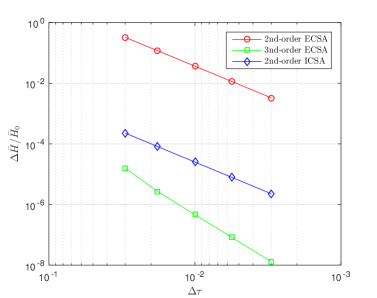
Figure 1: Convergence rate of the energy error for three symplectic methods. It verifies that $\Psi_{\Delta s}^{2}$ is indeed a second order method and $\Psi_{\Delta s}^{3}$ is a third order method.

III Numerical experiments

To demonstrate the long-term accuracy, conservativeness and efficiency of developed explicit symplectic algorithms for relativistic charged particle dynamics, we apply it to the secular runaway dynamics in tokamak. The electric and magnetic field are chosen to be

$$\begin{split}\mathbf{A}(\mathbf{x},t)&=\mathbf{A}_{0}(\mathbf{x})-\mathbf{E}(\mathbf{x})t\thinspace,\\ \mathbf{B}(\mathbf{x})&=\nabla\times\mathbf{A}_{0}(\mathbf{x})\thinspace,\\ \mathbf{E}(\mathbf{x})&=-E_{l}\dfrac{R_{0}}{R}e_{\zeta}\thinspace,\\ \mathbf{A}_{0}(\mathbf{x})&=\dfrac{B_{0}r^{2}}{2Rq}e_{\zeta}-\ln\left(\dfrac{R}{R_{0}}\right)\dfrac{R_{0}B_{0}}{2}e_{z}+\dfrac{B_{0}R_{0}z}{2R}e_{R}\,.\end{split}$$ (24)

where $R=\sqrt{x^{2}+y^{2}}$, $R_{0}$ is the major radius, $B_{0}$ is the magnetic field on axis, the constant $q$ is the safety factor, and $\zeta=arctan\left(\frac{x}{y}\right)$ is the toroidal coordinate of the torus. In this example, we take $R_{0}=1.7m$, $E_{l}=2V/m$ and $B_{0}=2T$ with $q=2$. The initial position and momentum of the runaway electron are $\mathbf{x}_{0}=(1.8,0,0)m$ and $\mathbf{p}_{0}=(3,10,0)m_{0}c$, where $c$ is the speed of light, and the proper time-step is set to be $\text{$\Delta$}s=0.03$. Displayed in Fig. 2 is the comparison of transit orbits calculated by the non-symplectic third order Runge-Kutta (RK3) method, second order implicit symplectic mid-point (2nd-order ICSA) method and the explicit second symplectic (2nd-order ECSA) algorithm $\Psi_{\Delta s}^{2}$. It is expected that after $4\times 10^{7}$ time steps, i.e. $1.136\times 10^{-4}$s, the width of transit orbits is almost the same with that of the initial orbits, since the diameter of gyromotion expressed by the width of orbit make little changing. Figure. 2(a) shows that the width of orbit obtained by the non-symplectic RK3 method after $4\times 10^{7}$ time steps is smaller than that of the initial one. The loss of the vertical momentum of runaway electron is mainly due to the accumulated numerical error of RK3. Meanwhile the orbits calculated by the 2nd-order ECSA method $\Psi_{\Delta t}^{2}$ in Fig. 2(b) and 2nd-order ICSA algorithm in Fig. 2(c) after $4\times 10^{7}$ time steps are almost the same with the initial one. The long-term relative mass-shell error by non-symplectic method gradually increases without bound due to numerical errors. On the contrary, for the symplectic integrators, the relative mass-shell errors are bounded by a small number for all time. This fact is clearly demonstrated in Fig. 2(d), where the mass-shell errors for the three algorithms are plotted.

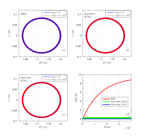
Figure 2: Simulations of long-term dynamics of a runaway electron in a tokamak. The initial orbits are plotted using blue lines, and the orbits after $4\times 10^{7}$ steps are plotted using red lines. (a) Numerical orbit obtained by a non-symplectic RK3 method. (b) The orbit obtained by the 2nd-order ECSA method. (c) The numerical orbit by the 2nd-order ICSA method. (d) The mass-shell error $\Delta\bar{H}/\bar{H}_{0}$ of three methods are plotted as functions of simulation time step.

To illustrate the efficiency of the explicit symplectic algorithms developed, the CPU time used by the three methods for calculating the charged particle dynamics is listed in Table. 1. The numerical calculation consists of $4\times 10^{6}$ time-steps, and is carried using on a Inter Core $i5-3210M$ CPU. It’s clear that the 2nd-order ECSA algorithm is much more efficient than the 2nd-order ICSA algorithm.

	RK3	2nd-order ICSA	2nd-order ECSA
CPU time (s)	6.628	29.886	14.801

Table 1: CPU time used by the three algorithms for runaway dynamics in a tokamak.

IV Conclusion

In this paper, we have constructed explicit symplectic algorithms for relativistic dynamics of charged particle by extending it into new variables $(\mathbf{x},\mathbf{p},t,p_{0})$ and combining the familiar sum-split method with generating function method. Notably, the developed methodology is expected to be applied to the relativistic dynamics of charged particle in Yang-Mills fields. In the future, the explicit symplectic simulation for Vlasov-Maxwell equations of relativistic charged particles will also be investigated based on the developed algorithms.