Statistical mechanics approach to lattice field theory

Abstract

The mean spherical approximation (MSA) is a closure relation for pair correlation functions (two-point functions) in statistical physics. It can be applied to a wide range of systems, is computationally fairly inexpensive, and — when properly applied and interpreted — lead to rather good results.

In this paper we promote its applicability to euclidean quantum field theories formulated on a lattice, by demonstrating how it can be used to locate the critical lines of a class of multi-component bosonic models. The MSA has the potential to handle models lacking a positive definite integration measure, which therefore are difficult to investigate by Monte-Carlo simulations.

1 Introduction

Perturbative quantum field theories (QFT), most notably Quantum Electrodynamics, belong to the most successful approaches in science. The agreement between the predicted and experimental values of the electron magnetic moment is probably the best verified number in physics. However, not all phenomena in this realm can be reliably analysed by weak-coupling perturbation theory, which anyway has some inherent limitations, due to its asymptotic nature and the fact that the expansion parameters are not always small.

It is not obvious how to proceed when perturbation theory fails, but one well established approach is to formulate an imaginary time version of the relevant model on a lattice, and study this system by Monte-Carlo simulations. Available computer memory and time impose (steadily increasing) limits on the size of the systems that can be treated by this method, and the accuracy of results. But there are also interesting quantum field models which are difficult to investigate by the Monte-Carlo method, due to lack of a positive definite probability measure.

In this paper we discuss a different approach to lattice field theory, using methods which have proven to work well in similar lattice models of statistical mechanics. Ultimately they also require numerical work, e.g. for the solution of integral equations. We will mostly focus on the MSA, which is a fairly simple method for approximating the pair correlation function (two-point function), and from this thermodynamic properties of the system under scrutiny.

MSA is exact for gaussian models, e.g. free field theories, and (for the type of models we consider) to first order of weak-coupling perturbation of these. It becomes exact for models with $N$-component fields as $N\to\infty$, and becomes better when the number of space-time dimensions $d$ increases. It is therefore expected to work better for $d=4$ QFT models than the $d=3$ models of statistical mechanics for which it was originally developed. It also becomes exact for long range interactions, more precisely to first order of the $\gamma$-expansion (although this is of less relevance for our approach in this work). Being constrained by exact limits in so many directions, the MSA have the prospects of being a quite relieable and useful additional tool for analysis of QFT models.

1.1 Summary of article

The rest of this paper is organized as follows:

• In section 2 we describe the models to be analyzed. First in section 2.1 as a formal functional integral over functions $\bm{\varphi}(\bm{x})$ defined on a $d$-dimensional euclidean space-time continuum. In section 2.2 this is formulated as a related integral over variables $\bm{\varphi}_{i}$ defined on a discrete $d$-dimensional hypercubic lattice; this can be interpreted as the partition function for a classical lattice spin model, with $N$-dimensional continuuous spins $\bm{s}_{i}$.

• In section 3 we reinterpret the lattice spin model as describing a mixture of classical particles confined to the sites of a lattice, with a hard-core interaction such that at most one particle can be at each site. The value of $\bm{s}_{i}$ specifies the type of particle at site $i$ (or if it is empty). In this interpretation the interacting part of the system Hamiltonian consists the off-diagonal terms of the lattice Laplace operator. In the absence of these terms the model becomes ultra-local; i.e. it reduces to a product of independent low-dimensional integrals, one for each lattice site. This zero’th order model, usually denoted the reference system, is discussed in section 3.1. Many quite successful nonperturbative methods for treating interactions have been developed for statistical mechanics of fluids. We describe some of them in section 3.2, including the $\gamma$-expansion, the mean spherical approximation (MSA), and the self-consistent Ornstein-Zernike approximation (SCOZA).

• Free quantum field theories are described by gaussian functional integrals, which therefore acts as the zero’th order model in standard QFT perturbation expansions, while it is already considered as an interacting model from our statistical mechanics viewpoint. To contrast the two approaches we therefore consider Gaussian models in section 4, for single-component fields in section 4.1, and generalized to multi-component fields in section 4.2.

• For QFT applications without lattice artifacts, a lattice model must be tuned to be very close to a second order critical point, so that all local quantities of interest have essentially infinite correlation lengths when measured in lattice units. Thus, the first task of any lattice approach is to locate the critical region. For the models considered explicitly in this paper, defined by Euclidean actions of the form

  $$S=-\sum_{ij}\frac{1}{2}\bm{\varphi}_{i}\Delta^{(L)}_{ij}\bm{\varphi}_{j}+\sum_{i}\frac{1}{2}m^{2}\bm{\varphi}^{2}_{i}+\frac{\lambda}{4!}\left(\bm{\varphi}^{2}_{i}\right)^{2},\quad\lambda\geq 0,$$ (1)

  this consists of a line $m^{2}(\lambda)$ in the $(m^{2},\lambda)$-plane, with $m^{2}\leq 0$ starting at $m^{2}=0$ for $\lambda=0$. In section 5 we calculate the three first terms of a perturbation expansion of this line, using standard weak-coupling QFT perturbation theory for $N$-component real fields.

• In section 6 we use spin model mean field theory (i.e., with averages computed in the ultra-local model) to compute an estimate of the critical line.

• In turns out that the results of the mean field calculations are easily adapted to the corresponding MSA calculations, performed in section 7, by simply replacing the space-time dimension $d$ by an effective dimension $d_{\text{eff}}$ (cf. figure 3). Mathematically the two quantities are related to the diagonal elements of the (inverse) lattice Laplace operators:

  $$1/(2d)=-\left[\Delta^{(L)}_{ii}\right]^{-1},\quad 1/(2d_{\text{eff}})=-\left[\Delta^{(L)}\right]^{-1}_{ii}\quad\text{(no sums over $i$)}.$$ (2)

  In section 7.1 we compare the weak coupling (small-$\lambda$) perturbation expansion of the MSA-result with the exact expansion of section 5. For the critical line, the MSA expansion is given by with the same diagrams, but with the full lattice propagator replaced by a constant. Contrary to the mean-field approximation the MSA is exact to first order in $\lambda$.

  In section 7.2 we perform a strong coupling (large-$\lambda$) perturbation expansion of the MSA-result, and find a surprising “duality” relation between coefficients of the weak and strong expansions, cf. eqs. (56). The leading order of the strong coupling expansion corresponds to the Ising limit, for which the $N=1$, $d=4$ critical point is known from Monte-Carlo simulations. The MSA results differs from this result by about $3.5\,\%$.

  In section 7.3 we perform a $1/N$ expansion of the MSA-result. The coefficients of this expansion exhibit an curious “duality” (anti-)symmetry, originating from the weak-strong relation mentioned above.

• Section 8 describes some of the numerical computations briefly and presents results for the critical line. Additional technical details are delegated to appendix A–D.

2 Functional integral description of quantum field theories

In this section we indicate briefly how bosonic quantum field theories (QFTs) can be formulated on a lattice, and interpreted as systems of continuous spins. As we will see in section 3, such systems can in turn be viewed as models for classical particles (lattice gases).

2.1 Formal continuum description

In QFT the grand partition function for a system in thermal equilibrium is formally given by a functional integral of the form,

$$\Xi=\text{e}^{\beta pV}=\int\text{e}^{-\frac{1}{\hbar c}\int^{\beta\hbar c}_{0}\int_{V}d^{d}x\,\mathcal{L}(\bm{\varphi},\partial\bm{\varphi})}\;\mathcal{D}\bm{\varphi},$$ (3)

where $\mathcal{L}$ is the Lagrangian of the QFT model, analytically continued to imaginary time, $x^{0}=\text{i}ct$, and $\beta=1/k_{B}T$. Here $V$ is the $(d-1)$-dimensional volume of space, assumed taken to infinity in a regular manner.

For bosonic fields eq. (3) is of a form similar to the continuum spin models we will discuss later (cf. sections 3 and 4), but with the important differences that

• the temperature variable is related to the extent of the imaginary time direction instead of being a parameter of the Lagrangian $\mathcal{L}$,

• chemical potentials are related to constant external gauge fields instead of local weight factors, $\partial/\partial x^{0}\equiv\partial_{0}\to\partial_{0}-\mu/(\hbar c)$. One can introduce an independent chemical potential for each independent conserved current in the QFT model; this has as consequence that the chemical potentials of particles and anti-particles must have opposite signs. This is a consequence of the fact that particles can be freely created and annihilated in relativistic QFT, only constrained by the conservation laws of the model.

• the QFT mean energy is different from the internal energy in the equivalent spin system.

The motivation/derivation of eq. (3) originates in the Feynman path integral formulation of quantum mechanics Feynman:1948ur ; Feynman:1949zx , and is exposed in depth in books like pathFeynman ; peskinqft ; critical:props:kleinert . We give a brief indication of how it can be derived in appendix A, with focus on the connection between the field theoretic and the conventional statistical mechanical description of the chemical potential.

In spin models, or the related lattice gas models for classical particles, the occurence of temperature and chemical potential parameters are entirely different. One must beware of the confusions which may arise when working and communicating from such disparate viewpoints.

In the remainder of this article we shall consider quantum systems at zero temperature and zero chemical potential, specified by functional integrals of the form

$$\Xi_{0}\left\{\mathbf{h}_{0}\right\}=\int\text{e}^{-\int{d}^{d}x\,\left[-\frac{1}{2}\bm{\varphi}_{0}\Delta\bm{\varphi}_{0}+\frac{1}{2}m_{0}^{2}\,\bm{\varphi}_{0}^{2}+\frac{1}{4!}\lambda_{0}\,\left(\bm{\varphi}_{0}^{2}\right)^{2}-\mathbf{h}_{0}\cdot\bm{\varphi}_{0}\right]}\;\mathcal{D}\bm{\varphi}_{0},$$ (4)

where $\Delta$ is the Laplace operator in $d$-dimensional Euclidean space. We will mostly focus on the case of $d=4$. In eq. (4) the parameter $m_{0}^{2}$ (‘bare mass’) may take negative values — which in fact is the most interesting case. The field $\bm{\varphi}_{0}$ have $N$ components (often referred to as spin dimension). In some calculations we will restrict $N$ to be a positive odd integer (even $N$ involves a different set of special functions).

2.2 Transformation to lattice formulation and spin model interpretation

To make the model amenable to the statistical mechanical approach of section 3, we restrict $x$ to the sites $x_{i}$ of a hypercubic lattice, with replacements $\int{d}^{d}x\to a^{d}\sum_{i}$ and $\Delta\to a^{-2}\Delta^{(\text{L})}$. Here $\Delta^{(\text{L})}$ is a corresponding dimensionless lattice Laplacian, with $a$ some characteristic lattice length — tiny relative to the scales of interest. By introducing new fields and parameters

$$\begin{split}\bm{\varphi}_{i}&=a^{(d-2)/2}\,\bm{\varphi}_{0}({x}_{i}),\quad m^{2}=a^{2}m_{0}^{2},\\ \lambda&=a^{(4-d)}\,\lambda_{0},\quad\mathbf{h}_{i}=a^{(d+2)/2}\,\mathbf{h}_{0}(x_{i})\end{split}$$ (5)

we obtain a lattice partition function

$$\Xi\left\{\mathbf{h}\right\}=\int\,\text{e}^{\frac{1}{2}\sum_{ij}\bm{\varphi}_{i}\Delta^{\text{(L)}}_{ij}\bm{\varphi}_{j}-\sum_{i}\left[\frac{1}{2}m^{2}\bm{\varphi}_{i}^{2}+\frac{1}{4!}\lambda{(\bm{\varphi}^{2}_{i})}^{2}-\mathbf{h}_{i}\cdot\bm{\varphi}_{i}\right]}\;\prod_{k}\frac{d\bm{\varphi}_{k}}{(2\pi)^{N/2}}.$$ (6)

This is similar to the partition functions for classical spin models investigated in statistical mechanics, most notably the Ising model, only in one dimension higher than usual, and with continuous (perhaps multidimensional) spins. We have a local factor for each site

$$f(\bm{\varphi}_{i})=(2\pi)^{-N/2}\,\text{e}^{-\frac{1}{2}(m^{2}+2d)\bm{\varphi}_{i}^{2}-\frac{1}{4!}\lambda(\bm{\varphi}_{i}^{2})^{2}+\mathbf{h}_{i}\cdot\bm{\varphi}_{i}},$$ (7)

plus nearest-neighbor ferromagnetic interactions $U=-\sum_{\langle ij\rangle}\bm{\varphi}_{i}\cdot\bm{\varphi}_{j}$, where the sum runs over all nearest-neighbor pairs (“hopping Hamiltonian”), corresponding to the standard numerical $(2d+1)$-stensil approximation of the Laplace operator. By our statistical mechanical approach we will focus upon and utilize the MSA (mean spherical approximation) which is defined and explained in section 3. For our MSA approach this particular form of $U$ is not important; the important feature is that it can be expressed as a translation invariant sum of quadratic pair interactions, $U=-\sum_{\langle ij\rangle}\bm{\varphi}_{i}\,\bm{\psi}(\mathbf{r}_{ij})\,\bm{\varphi}_{j}$. Since a term of the form $\frac{1}{2}\sum_{i}\bm{\varphi}_{i}\,\mathbf{c}_{0}\,\bm{\varphi}_{i}$ is both quadratic and local, we have the freedom to multiply $f(\bm{\varphi}_{i})$ by the factor $\text{e}^{-\frac{1}{2}\bm{\varphi}_{i}\mathbf{c}_{0}\,\bm{\varphi}_{i}}$, while changing $U\to U-\frac{1}{2}\sum_{i}\bm{\varphi}_{i}\mathbf{c}_{0}\,\bm{\varphi}_{i}$ at the same time. This freedom is the most crucial part of the MSA; it resembles the procedure of adding mass counterterms in standard renormalized QFT perturbation theory.

In the spin formulation the corresponding inverse temperature $\beta$ set to unity. This is different from the QFT $\beta$ of eq. (3). For greater resemblance with statistical systems one may make a scale transformation of the fields, $\bm{\varphi}_{i}=\sqrt{\beta}\,\bm{s}_{i}$, to eliminate one combination of the local parameters ($m^{2}$ and $\lambda$) in favor of a temperature-like variable. This is useful to simplify comparison with known results in the Ising limit, $\bm{s}^{2}_{i}=1$.

3 Lattice gas mixtures

In this section we discuss the connection between spin models (also known as bosonic QFTs) and multicomponent mixtures of classical particles. It is well known that the Ising model can be regarded as a lattice gas, i.e. a gas of classical particles confined to the sites $i$ of a lattice, where Ising spin $s_{i}=1$ defines the presence of a particle on site $i$, and $s_{i}=-1$ that site $i$ is empty. Note that $i$ may label the sites of a multidimensional lattice; hence it is naturally viewed as an index vector, but to simplify notation we do not write this explicitly. The Ising model can be extended to spins taking more that two values, and eventually to continuous spins. Such systems can be regarded as mixtures of classical particles confined to the sites of a lattice (i.e., lattice gas mixtures). The advantage of employing this equivalence is that physical intuition, together with some powerful methods developed for analysis of classical fluids, can be applied fruitfully. Such an approach was used by Høye and Stell in a previous study of continuous spins hoye97 . Here we will use it to study continuous spins in four spatial dimensions.

In the lattice gas interpretation the density of particles of type $s$ at a given site $i$ is

$$\rho_{s}=\langle n_{s}\rangle,$$ (8)

where the set of particle numbers at that site, $\left\{n_{s}\right\}$, is restricted by the hard core condition, $\sum_{s\neq 0}n_{s}\leq 1$, preventing multiple occupancy of cells. Here an empty site (vacuum state) is specified by $n_{0}=1$. Therefore, the configuration at site $i$ is uniquely specified by the value of $s$ for which $n_{s}=1$. With discrete spins the $s$ takes discrete values, but we will eventually let $s$ be a continuous variable.

Consider a lattice gas mixture in $d$ dimensions, where the lattice is taken to be simple cubic. The particles of type $s$ have a chemical potential $\mu_{s}$. With the equivalent spin systems in mind, the fugacity in general can be written as

$$z_{s}=e^{\beta\mu_{s}}=f(s)\,\text{e}^{\beta{\cal H}s},$$ (9)

where ${\cal H}$ is the applied magnetic field, $\beta=1/(k_{B}T)$, $T$ is temperature, and $k_{B}$ is Boltzmann’s constant. By specifying $z_{0}=f(0)=1$, the vacuum state is normalized to have zero “chemical potential”, $\mu_{0}=0$.

In the lattice gas interpretation the (grand) partition function for this system is identified by the thermodynamic pressure $p$, $Z_{g}=\text{e}^{\mathcal{N}\beta p}$, where $\mathcal{N}$ is the number of lattice sites. We associate each site with a cell of unit volume. In this representation the thermodynamic potential $\beta p$ is viewed as a function of the chemical potentials $\beta\mu_{s}$. For later statistical mechanical evaluations it is convenient to make a Legendre transformation to new independent variables and a new thermodynamic potential,

$$\rho_{s} =\frac{\partial(\beta p)}{\partial(\beta\mu_{s})},$$ (10a)

$$I =\beta p-\sum_{s}\beta\mu_{s}\rho_{s}=\Big{(}1-\sum_{s}\beta\mu_{s}\frac{\partial}{\partial(\beta\mu_{s})}\Big{)}\beta p=-\beta F.$$ (10b)

Here $F=U-TS$ is the Helmholtz free energy per site, where $U$ is the (configurational) internal energy per site and $S$ is the corresponding entropy.

3.1 The reference system

We will consider expansions around a zero’th order system, the reference system, where there is no interaction between particles at different sites. This is different from the free field (gaussian) models commonly used as zero’th order systems in QFTs. We will denote quantities related to the reference system by the subscript $R$. The grand partition function per site is simply

$$Z_{g}=\text{e}^{\beta p_{R}}=\mathop{{\sum}^{\prime}}_{\left\{n_{s}\geq 0\right\}}\text{e}^{\beta\mu_{s}n_{s}}=\sum_{s}z_{s}.$$ (11)

Here the first sum is restricted by the hard core condition, $\sum_{s\neq 0}n_{s}\leq 1$. This leads to the second sum. In the limit of continous spins the second sum should be replaced by a corresponding integral over $s$. The average particle densities become

$$\rho_{s}=\frac{\partial\ln Z_{g}}{\partial(\beta\mu_{s})}=\frac{z_{s}}{Z_{g}}.$$ (12)

From this follows the pressure $p_{R}$ of the reference system hard core lattice gas,

$$\beta p_{R}=\ln Z_{g}=\ln(z_{0}/\rho_{0})=-\ln\rho_{0}=-\ln(1-\rho),$$ (13)

with total density $\rho=\sum_{s\neq 0}\rho_{s}$, and $\rho_{0}$ the density of empty sites. At low total density this reduces to the ideal gas law. For a Legendre transformation we use eqs. (12)–(13) to express the chemical potentials in terms of densities,

$$\beta\mu_{s}=\ln\frac{\rho_{s}}{\rho_{0}},$$ (14a)

which gives

$$I_{R}\equiv-\beta F_{R}=-\sum_{s\neq 0}\rho_{s}\ln\rho_{s}-\rho_{0}\ln\rho_{0}.$$ (14b)

From these results one may verify the thermodynamic relations,

$$\beta\mu_{s} =-\frac{\partial I_{R}}{\partial\rho_{s}},$$ (15a)

$$G_{R} =\sum_{s\neq 0}\rho_{s}\mu_{s}=F_{R}+p_{R},$$ (15b)

where $G_{R}$ is the Gibbs free energy per site for the reference system.

For the expansion in section 3.2, some correlation functions of the reference system are also needed. Since there are no interactions between different sites, these functions are ultra-local. The quantities of interest are

$$\sum_{s}\,\langle n_{s}\rangle s =\sum_{s}\rho_{s}\,s=\langle s\rangle\equiv{\,\texttt{m}},$$ (16a)

$$\sum_{ss^{\prime}}\langle n_{s}n_{s^{\prime}}\rangle\,ss^{\prime} =\sum_{ss^{\prime}}\rho_{s}\delta_{ss^{\prime}}\,ss^{\prime}=\langle s^{2}\rangle,$$ (16b)

or more precisely in the combination

$$R\equiv\langle s^{2}\rangle-{\,\texttt{m}}^{2}.$$ (16c)

The first equality in eq. (16b) follows from the hard core condition, which implies that $n_{s}n_{s^{\prime}}=n_{s}\delta_{ss^{\prime}}$.

3.2 Interacting systems and the $\gamma$-expansion

The spins or lattice gas particles may interact. The usual form of this interaction is a sum of pair interactions of the Heisenberg form,

$$U=\frac{1}{2}\sum_{ij}\sum_{s_{i},s_{j}}n_{s_{i}}(i)\,n_{s_{j}}(j)\,\psi({\bf r}_{ij})s_{i}s_{j}=\frac{1}{2}\sum_{i,j}\psi({\bf r}_{ij})s_{i}s_{j},$$ (17)

with $\psi(\mathbf{0})=0$, and where $\psi<0$ for ferromagnetic interactions. Here ${\bf r}_{ij}={\bf r}_{i}-{\bf r}_{j}$ is the relative separation between spins $i$ and $j$. The hard core interaction that prevents multiple occupancy is similar to the hard cores of molecules in classical fluids. When the interaction (17) is turned on, the $s$-dependence of the density distribution (12) will change. For the Ising model there is no such change for a given magnetization, since it corresponds to a one component lattice gas (with only two possible states at each site). However, for the more general situation a satisfactory approximation of the resulting $s$-dependence is crucial.

Similar to classical fluids, the solution of the spin problem with non-zero interactions (17) cannot be done exactly (with a few exceptions, mostly in one and two dimensions). Thus, one has to make approximations, usually described by a sum of graphs. E.g. to go beyond a pure density expansion, some organizing principle for summing classes of graphs is required. One such principle is the $\gamma$-ordering scheme by Hemmer Hemmer64 and Lebowitz et. al. Lebowitz65 , where one makes the replacement

$$\psi(\textbf{r}_{ij})\rightarrow\gamma^{d}\,\psi(\gamma\textbf{r}_{ij})$$

in eq. (17), continues with a systematic expansion around $\gamma=0$, and (for a concrete physical system) sets $\gamma=1$ in the end. The resulting organization of diagrams has close similarity to the loop (or $\hbar$) expansion in quantum field theory. The leading contribution is the mean field approximation, which becomes exact in the limit $\gamma\rightarrow 0$.

In terms of the statistical mechanical graph expansion of the free energy as function of densities, the whole mean field contribution is given by a single potential bond, i.e.

$$\begin{split}I_{MF}&=I_{R}+\frac{1}{2\mathcal{N}}\sum_{i,j}\sum_{s_{i},s_{j}}\rho_{s_{i}}\rho_{s_{j}}v(\mathbf{r}_{ij})s_{i}s_{j}\\ &=I_{R}+\frac{1}{2}{\,\texttt{m}}^{2}\,\tilde{v}(\mathbf{0}).\end{split}$$ (18)

We have assumed the densities $\rho_{s}$ to be independent of position. The tilde designates a $d$-dimensional Fourier transformed function,

$$\begin{split}\tilde{v}(\mathbf{k})&=\sum_{j}v(\mathbf{r}_{0j})\,\text{e}^{\text{i}\mathbf{k}\cdot\mathbf{r}_{0j}},\\ v(\mathbf{r})&=\frac{1}{(2\pi)^{d}}\int_{-\pi}^{\pi}\cdots\int_{-\pi}^{\pi}\,\tilde{v}(\mathbf{k})\,\text{e}^{\text{i}\mathbf{k}\cdot\mathbf{r}}d\mathbf{k}.\end{split}$$ (19)

$$\tilde{v}(\mathbf{k})=c_{0}-\beta\tilde{\psi}({\bf k}).$$ (20)

An adjustable parameter, $v(\mathbf{0})\equiv c_{0}$ (with $\psi(\mathbf{0})=0$), has now been introduced. The $c_{0}$ corresponds to a finite particle-particle interaction inside the hard cores ($\mathbf{r}=\mathbf{0}$). This does not influence the exact physics of the system, since two particles cannot be at the same site.

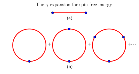
Figure 1: Diagrams for the first two terms of the $\gamma$-expansion. A potential bond (red line) represents the function $v(\textbf{r}_{ij})\,s_{i}s_{j}\equiv[c_{0}\delta_{ij}-\beta\psi(\textbf{r}_{ij})]\,s_{i}s_{j}$ in real space, and each vertex (filled, blue circle) represents a summation $\sum_{s}\sum_{s^{\prime}}s\tilde{\Gamma}_{0ss^{\prime}}s^{\prime}$ where $s$ and $s^{\prime}$ are the endpoints of potential bonds on each side of the vertex.

The first correction to the mean field approximation is given by the ring graphs, see figure 1(b), whose sum is

$$I_{M1}=-\frac{1}{2(2\pi)^{d}}\int_{-\pi}^{\pi}\cdots\int_{-\pi}^{\pi}\,\ln(1-R\tilde{v}(\mathbf{k}))\,d\mathbf{k}.$$ (21)

However, with the particle picture one has to show a bit care here since $c_{0}$ varies. Then a potential bond should not return to the same $\rho_{s}$ vertex. This means that the $\rho_{s}\delta_{ss^{\prime}}$ and $\langle s^{2}\rangle$ terms of eqs. (23) and (24) below should not contribute in the first ring graph (with one blue circle) of figure 1. Thus this should be compensated by which the particle picture contribution to the free energy is ($\psi(\mathbf{0})=0$)

$$I_{1} = I_{M1}-\frac{1}{2}c_{0}\langle s^{2}\rangle=I_{M1}-\frac{1}{2}c_{0}(R+{\,\texttt{m}}^{2})$$ (22)

$$= I_{M1}-\frac{1}{2(2\pi)^{3}}\int R\tilde{v}(\mathbf{k})\,d\mathbf{k}-\frac{1}{2}c_{0}{\,\texttt{m}}^{2}.$$

This result is also consistent with the thermodynamics of the MSA obtained in ref. hoye77 . The result for $I_{1}$ is the same as for graph expansion with $c_{0}$ constant. A reason for this is that first partial derivatives with respect to $c_{0}$ (and thus $R$) will cancel as seen below where the equation of state is found via the chemical potentials $\mu_{s}$.

The constant $R$ in eqs. (21) and (22) represents local (hyper-)vertices in the ring graphs, where pairs of potential bonds meet. The $s$-dependences of their endpoints are summed (averaged) over the reference system pair correlation functions that also includes self-correlations ($\rho$-vertex). They are

$$\tilde{\Gamma}_{0ss^{\prime}}({\bf k})=\Gamma_{0ss^{\prime}}(0)=\rho_{s}\delta_{ss^{\prime}}-\rho_{s}\rho_{s^{\prime}}$$ (23)

since $\Gamma_{0ss^{\prime}}({\bf r})=0$ otherwise. The last term of this equation expresses the hard core condition that prohibits more than one particle to occupy a cell (i.e. zero minus the ideal gas probability). With this one gets

$$\begin{split}R&=\sum_{ss^{\prime}}ss^{\prime}\Gamma_{0ss^{\prime}}(0)=\langle s^{2}\rangle-{\,\texttt{m}}^{2},\\ {\,\texttt{m}}&=\langle s\rangle=\sum_{s}s\rho_{s},\end{split}$$ (24)

where  m is average magnetization.

Now we can find the leading contribution to the resulting pair correlation function with $U\neq 0$. It is formed by chain graphs where $\tilde{v}({\bf k})$-bonds are connected by hypervertices. Its average when including the reference piece (24) is

$$\tilde{\Gamma}({\bf k})=\frac{R}{1-R\tilde{v}({\bf k})}.$$ (25)

We can now optimize the value of the parameter $c_{0}$ such that the exact core condition expressed by eq. (23) also is fulfilled by the resulting correlation function. With the average (24) this implies the condition

$$R=\Gamma(\mathbf{0})=\frac{1}{(2\pi)^{d}}\int\tilde{\Gamma}({\bf k})\,d{\bf k}.$$ (26)

Due to this condition the resulting contribution to the chemical potential from the $I_{1}$ of eq. (22) simplifies; so it becomes

$$\beta\mu_{1s}=-\frac{\partial I_{1}}{\partial\rho_{s}}=-c_{0}{\,\texttt{m}}s+\frac{1}{2}c_{0}s^{2}.$$ (27)

This follows from $\partial R/\partial\rho_{s}=s^{2}-2{\,\texttt{m}}s$ with $R$ given by eq. (24). Further, differentiation of $c_{0}$ does not contribute due to condition (26) hoye77 . The same is the situation for $R$ except for the last term of eq. (21) which results in $\tilde{v}(\mathbf{k})\rightarrow v(\mathbf{0})=c_{0}-\beta\psi(\mathbf{0})=c_{0}$. Altogether, including result (27), the mean field contribution from eq. (18), and the reference system contribution (14a) the resulting chemical potentials become

$$\beta\mu_{s}=\ln\left(\frac{\rho_{s}}{\rho_{0}}\right)-[c_{0}-\beta\tilde{\psi}(\mathbf{0})]{\,\texttt{m}}s+\frac{1}{2}c_{0}s^{2}.$$ (28)

When inserted in eq. (9) one finds the resulting density or effective spin distribution

$$z_{es}=\frac{\rho_{s}}{\rho_{0}}=f_{e}(s)e^{\beta{\cal H}_{e}s}$$ (29)

with

$$\beta{\cal H}_{e}=\beta{\cal H}+[c_{0}-\beta\tilde{\psi}(0)]{\,\texttt{m}},\quad f_{e}(s)=f(s)e^{-c_{0}s^{2}/2}.$$ (30)

This equation also gives the equation of state ${\cal H}={\cal H}({\,\texttt{m}})$ where ${\cal H}_{e}={\cal H}_{e}({\,\texttt{m}})$ is the equation of state for free spins that follows from eq. (29) alone.

The above expressions with $c_{0}$ determined via the exact core condition as expressed by eq. (26) is the MSA (mean spherical approximation) extended to mixtures where $\langle s^{2}\rangle$ is not fixed. Its equation of state as a magnetic spin system is in the MSA given by eq. (30).

The MSA, which is consistent with $\gamma$-expansion, has its origin in the SM (spherical model) that was solved by Berlin and Kac as an approximation to the Ising model berlin52 . In the SM the values of the spins are not restricted to $\pm 1$; instead the sum of their values squared are fixed. This was modified by Lewis and Wannier to the MSM (mean SM) where the average of the spin values squared are fixed lewis52 . This is equivalent to a Gaussian model with adjustable one-particle potential to keep $\langle s_{i}^{2}\rangle=1$ fixed. Then the MSM was extended to continuum fluids by Lebowitz and Percus lebowitz66 . This extension was the basis of the MSA with correlation function eq. (25) and core condition eq. (26) in the present case. With the MSA the reference system is defined to be the one of non-interacting Ising spins. The MSM is different in this respect. In section 3.2 the MSA is extended to a more general spin system. (However, since we in this work only need to consider ${\,\texttt{m}}=0$, the difference from MSA is not significant.)

From eq. (30) one can evaluate the inverse susceptibility $\chi^{-1}$

$$\beta\chi^{-1}=\frac{\partial{\cal H}}{\partial{\,\texttt{m}}}=\frac{1}{R}-\tilde{v}(\mathbf{0})-\frac{\partial c_{0}}{\partial{\,\texttt{m}}}{\,\texttt{m}}$$ (31)

with $\partial(\beta{\cal H}_{e})/\partial{\,\texttt{m}}=1/R$. According to the fluctuation theorem one should have $\beta\chi^{-1}=\Gamma(0)^{-1}$. Expression (31) deviates from this by the term   $-(\partial c_{0}/\partial{\,\texttt{m}}){\,\texttt{m}}$. Such deviations are typical for any approximation and is some measure of its accuracy. This inaccuracy can be removed by the SCOZA (self-consistent Ornstein-Zernike approximation) where a free parameter like effective temperature is used hoye84 ; hoye85 . The latter has lead to very accurate results for instance for the Ising model in one, two, and three dimensions. Accurate numerical SCOZA data for the Ising model was initially obtained by Dickman and Stell dickman96 . With nearest neighbor interaction it is exact in one dimension. In two dimensions the sharp phase transition is missing, but otherwise the results are very accurate when compared with the known exact solution for ${\,\texttt{m}}=0$ hoye98 .

Later a variety of accurate SCOZA results have been obtained. Various references to such results can be found in the work by Høye and Lomba in their detailed investigation of the critical properties of another related accurate theory, the HRT (hierarchical reference theory) (in three spatial dimensions) hoye11 . They found that the critical indices turned out to be simple rational numbers. Recently this analysis of the HRT was extended to spins of dimensionality ${N}$, and they found by analysis in view of SCOZA and detailed numerical work that critical indices were independent of ${N}$ lomba14 . This contrasts earlier HRT results and other previous results from renormalization group theory where indices are expected to vary with ${N}$ parola12 ; fisher72 . The reason for rational numbers and independence upon ${N}$ (for ${N}$ finite) of the critical indices is the found connection between a leading and two subleading layers of contributions to the critical behavior. These layers are connected to each other and mean field behavior away from the critical point by which rational numbers for the critical indices appear. (However, the indices with good accuracy may effectively vary with ${N}$ when results are fitted to an assumed single power.) lomba14 .

The HRT, based upon the momentum space renormalization group theory, developed by Wilson and Kogut wilson74 , was introduced and studied by Parola and Reatto parola85 . However, the SCOZA method, which was extended to continuous spins in ref. hoye97 , will not be pursued further in this work.

4 The Gaussian model

It may be instructive see how the method of section 3 works on an explicitly solvable example, the Gaussian model. Essentially, this model is just a different name for a free bosonic lattice field theory (allowing for a more general Hamiltonian), but viewed and analysed from the perspective of statistical mechanics. The partition function and all correlation functions are in principle straightforward to calculate by doing gaussian integrals. In this section we want to reconstruct these results. In section 4.1 we discuss this model for the case of a one-dimensional continuous spin $s$ (single-component field), as in section 3. In section 4.2 we generalize to an $N$-dimensional continuous spin (multi-component field).

4.1 Single-component field (one-dimensional spin)

This model is defined by the quadratic form

$$\beta H=\frac{1}{2}\sum_{i,j}{s}_{i}\mathcal{K}(\textbf{r}_{ij}){s}_{j}-\beta\mathcal{H}\sum_{i}s_{i},$$ (32)

where each $s_{i}$ take continuous values in the range $\left(-\infty,\infty\right)$, and

$$\mathcal{K}_{ij}\equiv\mathcal{K}(\textbf{r}_{ij})=R_{0}^{-1}\delta_{ij}+\beta\psi(\textbf{r}_{ij})$$ (33)

is a positive definite matrix which we have decomposed into a local term, $R_{0}^{-1}\delta_{ij}$, and an interaction term, $\psi_{ij}\equiv\psi(\textbf{r}_{ij})$ with $\psi(\mathbf{0})=0$. The partition function and lowest order correlation functions for a number of $\mathcal{N}$ sites evaluates to (with $\int\mathcal{D}s\equiv\prod_{k}\int_{-\infty}^{\infty}ds_{k}/\sqrt{2\pi}$) ($\psi_{ij}\rightarrow\psi$ with matrix $\psi$),

$$\text{e}^{\mathcal{N}\beta p} =\int\mathcal{D}s\,\text{e}^{-\frac{1}{2}\sum_{ij}s_{i}\left(R_{0}^{-1}+\beta\psi\right)_{ij}s_{j}+\beta\mathcal{H}\sum_{i}s_{i}}$$

$$=\det{}^{-1/2}\left(R_{0}^{-1}+\beta\psi\right)\,\text{e}^{\frac{1}{2}\mathcal{N}\left[R_{0}^{-1}+\beta\tilde{\psi}(\mathbf{0})\right]^{-1}\,(\beta\mathcal{H})^{2}}$$

$$=\det{}^{-1/2}\left(R_{0}^{-1}+\beta\psi\right)\,\text{e}^{\frac{1}{2}\mathcal{N}\left[R_{0}^{-1}+\beta\tilde{\psi}(\mathbf{0})\right]\,m^{2}},$$ (34a)

m $$\equiv\langle s_{i}\rangle=\big{[}{R_{0}^{-1}+\beta\tilde{\psi}(\mathbf{0})}\big{]}^{-1}\,\beta\mathcal{H},$$ (34b)

$$\Gamma(\textbf{r}_{ij}) \equiv\langle s_{i}s_{j}\rangle-\langle s_{i}\rangle\langle s_{j}\rangle=\big{(}{R_{0}^{-1}+\beta\tilde{\psi}(\mathbf{0})}\big{)}^{-1}_{ij}.$$ (34c)

The contribution from the determinant in eq. (34a) can be written as

$$\log\det{}^{-1/2}\left(R_{0}^{-1}+\beta\psi\right)$$

$$=\frac{\mathcal{N}}{2}\log R_{0}-\frac{\mathcal{N}}{2(2\pi)^{d}}\int_{-\pi}^{\pi}\cdots\int_{-\pi}^{\pi}\log\left[1-R_{0}(-\beta\tilde{\psi})(\mathbf{k})\right]\,d\bf{k}.$$ (35)

All higher order correlators can be constructed from  m and $\Gamma$ by use of Wick’s theorem. Further, all subsets of the $s$-variables are gaussian distributed, with parameters which can be found from the expressions above. In particular, the $s$-distribution at each single site is found to be

$$\rho_{s}=\frac{1}{\sqrt{\Gamma(\mathbf{0})}}\,\text{e}^{-\frac{1}{2}(s-{\,\texttt{m}})^{2}/\Gamma(\mathbf{0})}.$$ (36)

when the “normalization” $\sum_{s}\rho_{s}\rightarrow\int\rho_{s}\,ds/\sqrt{2\pi}$ like the one in eq. (34a) is used.

Then we will test the lattice gas method on the Gaussian model. The given spin distribution will be $f(s)=e^{-s^{2}/(2R_{0})}$. With the MSA the effective spin distribution and equation of state are given by eqs. (29) and (30). Thus $f_{e}(s)=\exp[-(R_{0}^{-1}+c_{0})s^{2}/2]$, and accordingly

$${R}^{-1}={R_{0}}^{-1}+c_{0}.$$ (37)

By insertion of expression (37) into eq. (25) the exact correlation function (34c) is recovered. Further by computing the equation for $\beta{\cal H}_{e}({\,\texttt{m}})$ for the reference system from $f_{e}(s)$ one finds

$$\beta{\cal H}_{e}={\,\texttt{m}}/R={\,\texttt{m}}/R_{0}+c_{0}{\,\texttt{m}}$$ (38)

(i.e. eq. (34b) with $R_{0}\rightarrow R$ and $\psi=0$). When inserted in eq. (30) the exact result (34b) for  m is recovered. With spin distribution (29) the exact one (36) is also recovered when $R=\Gamma(\mathbf{0})$ from eq. (26) is used.

The gaussiam model partition function can also be found by use of the MSA. This is done in Appendix B where the exact result (34a) is recovered.

Altogether we have found that the MSA solves the gaussian model exactly for any pair interaction (17). For other situations it becomes exact in the mean field limit $\gamma\rightarrow 0$ where $\gamma$ is the inverse range of interaction. Finally it becomes exact in the limit $N\rightarrow\infty$ for spins of dimensionality $N$ YanWannier65 ; hoye1997Ddim . The latter is equivalent to the MSM (mean spherical model) which has been generalized to the GMSM (generalized MSM) hoye07 .

4.2 Multi-component field ($N$-dimensional spins)

The generalization to multi-component gaussian fields is mostly a change of notation. The quadratic form becomes

$$\beta H=\frac{1}{2}\sum_{i,j}\bm{s}_{i}\big{[}\mathbf{R}_{0}^{-1}\delta_{ij}+\beta\mathbf{\psi}(\bm{r}_{ij})\big{]}\bm{s}_{j}-\beta\bm{\mathcal{H}}\cdot\sum_{i}\bm{s}_{i},$$ (39)

where each $\bm{s}_{i}$ and $\bm{\mathcal{H}}$ are $N$-component real vectors, $\mathbf{R}$ is a real symmetric positive definite $N\times N$ matrix, and $\mathbf{v}(\bm{r})$ is a real matrix-valued function (symmetric $N\times N$ matrices). With $\int(\cdots)\mathcal{D}\bm{s}\equiv\prod_{k}\int_{-\infty}^{\infty}(\cdots){d\bm{s}_{k}}/{({2\pi})^{N/2}}$ the partition function, and associated correlation functions, evaluates to

$$\text{e}^{\mathcal{N}\beta p} =\int\text{e}^{-\frac{1}{2}\sum_{ij}\bm{s}_{i}\left[\mathbf{R}_{0}^{-1}+\beta\mathbf{\psi}\right]_{ij}\bm{s}_{j}+\beta\bm{\mathcal{H}}\cdot\sum_{i}\bm{s}_{i}}\;\mathcal{D}\bm{s}$$

$$=\det{}^{-1/2}(\mathbf{R}_{0}^{-1}+\beta\mathbf{\psi})\,\text{e}^{\frac{1}{2}\mathcal{N}(\beta\bm{\mathcal{H}})[\mathbf{R}_{0}^{-1}+\beta\mathbf{\tilde{\psi}}(\bm{0})]^{-1}(\beta\bm{\mathcal{H}})}$$

$$=\det{}^{-1/2}(\mathbf{R}_{0}^{-1}+\beta\mathbf{\psi})\,\text{e}^{\frac{1}{2}\mathcal{N}\bm{m}\,[\mathbf{R}_{0}^{-1}+\beta\mathbf{\tilde{\psi}}(\bm{0})]\,\bm{m}},$$ (40a)

$$\bm{m} =\langle\bm{s}_{i}\rangle=\big{[}\mathbf{R}_{0}^{-1}+\beta\mathbf{\tilde{\psi}}(\bm{0})\big{]}^{-1}\beta\bm{\mathcal{H}},$$ (40b)

$$\bm{\Gamma}(\mathbf{r}_{ij}) =\langle\bm{s}_{i}\bm{s}_{j}\rangle-\langle\bm{s}_{i}\rangle\langle\bm{s}_{j}\rangle=\left[\mathbf{R}_{0}^{-1}+\beta\mathbf{\psi}\right]^{-1}_{ij}.$$ (40c)

The $\bm{s}$-distribution at each single site is similar to eq. (36)

$$\rho_{\bm{s}}=\det\big{[}\bm{\Gamma}(\mathbf{0})\big{]}^{-1/2}\,\text{e}^{-\frac{1}{2}(\bm{s}-\bm{m}){\bm{\Gamma}(\bm{0})}^{-1}(\bm{s}-\bm{m})}.$$ (41)

As we did for the single-component gaussian model above, one can again perform the MSA evaluations to recover the exact solution.

5 Perturbation expansion for the critical line

For later comparison, we shall in this section compute the critical line for small values of $\lambda$ by the renormalized field theoretic perturbation method. The requirement of infinitely long-range correlations is that the renormalized mass $m^{2}_{r}$ vanishes,

$$m^{2}_{r}=m^{2}+\delta m^{2}(\lambda)=0.$$ (42)

Hence, we use $-\frac{1}{2}\sum_{ij}\bm{\varphi}_{i}\Delta^{\text{(L)}}_{ij}\bm{\varphi}_{j}$ as the $0^{\text{th}}$ order Hamiltonian (we do not use a renormalized field $\bm{\varphi}$). This gives a $0^{\text{th}}$ order lattice propagator,

$$\mathbf{G}^{(0)}_{ab}(\bm{x};m^{2}) =\delta_{ab}\,\frac{1}{V_{\text{BZ}}}\int_{\text{BZ}}\frac{\text{e}^{\text{i}\bm{k}\cdot\bm{x}}}{m^{2}+2d-2\sum_{n=1}^{d}\cos(k_{n})}\;\text{d}\bm{k}$$

$$=\delta_{ab}\,\int_{0}^{\infty}\text{e}^{-m^{2}t}\,\prod_{n=1}^{d}\text{e}^{-2t}\,I_{x_{n}}(2t)\,\text{d}t,$$ (43)

where the last integral follows from appendix C.

Next compute the self-energy correction $\mathbf{\tilde{\Sigma}}(\bm{p};\lambda)$ to $\mathbf{G}(\bm{x}_{ij};m^{2},\lambda)\equiv\langle\bm{\varphi}_{i}\bm{\varphi}_{j}\rangle$ in powers of $\lambda$, and choose $m^{2}$ order by order in $\lambda$ such that eq. (42) is fulfilled. The Feynman diagrams for $\mathbf{\tilde{\Sigma}}(\bm{p})$ are shown in figure 2. This determines the critical values of $m^{2}$ to

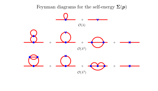
Figure 2: Self-energy diagrams to third order in $\lambda$. There is an overall minus-sign, and a factor $-\lambda$ for each ordinary vertex. The $m^{2}$-contributions (last term of each line) is chosen such that the contributions of each line vanishes at $\bm{p}=\bm{0}$. Due to this condition the first two terms on the $\mathcal{O}(\lambda^{2})$-line cancel exactly. There is a similar cancelation between tadpole terms of order $\lambda^{3}$; we have not drawn the cancelling diagrams on the $\mathcal{O}(\lambda^{3})$-line. For $N=1$ the combinatorial factors are given directly by the symmetry factors of each diagram. For larger $N$ one may rewrite $\frac{\lambda}{4!}(\bm{\varphi}^{2})^{2}=\frac{\lambda}{4!}\sum_{a}\varphi^{4}_{a}+\frac{\lambda^{\prime}}{2!^{3}}\sum_{a\neq b}\varphi^{2}_{a}\varphi^{2}_{b}$, with $\lambda^{\prime}=\frac{1}{3}\lambda$, and use the symmetry factors of a larger set of diagrams with the same topology, but propagators of different colors.

$$m^{2}= -{\textstyle\frac{(N+2)}{6}}\lambda\,G^{(0)}(\bm{0};0)+{\textstyle\frac{(N+2)}{18}}\lambda^{2}\sum_{i}{G^{(0)}(\bm{x}_{i};0)}^{3}$$

$$-{\textstyle\frac{(N+2)^{2}}{108}}\lambda^{3}\sum_{i}G^{(0)}(\bm{x}_{i};0)^{3}\sum_{j}G^{(0)}(\bm{x}_{j};0)\left[G^{(0)}(\bm{x}_{j}+\bm{x}_{i};0)-G^{(0)}(\bm{x}_{j};0)\right]$$

$$-{\textstyle\frac{(N+2)(N+8)}{108}}\lambda^{3}\sum_{i}G^{(0)}(\bm{x}_{i};0)^{2}\sum_{j}G^{(0)}(\bm{x}_{j};0)^{2}\,G^{(0)}(\bm{x}_{i}+\bm{x}_{j};0)$$ (44a)

$$= -{\textstyle\frac{(N+2)}{6}}\lambda\,a_{1}+{\textstyle\frac{(N+2)}{18}}\lambda^{2}\,a_{2}-{\textstyle\frac{(N+2)^{2}}{108}}\lambda^{3}\,a_{3a}-{\textstyle\frac{(N+2)(N+8)}{108}}\lambda^{3}\,a_{3b}.$$ (44b)

The terms in eq. (44a) are combined such that all sums are convergent. Numerical evaluation of the sums (rather crude for the higher order diagrams) gives

$$a_{1} =\phantom{-}0.154\,933\,390\,231\,060\,214\,084\,837\,208\ldots$$

$$a_{2} =\phantom{-}0.004\,043\,054\,812\,2\ldots$$

$$a_{3a} =-0.000\,007\,513\ldots$$

$$a_{3b} =\phantom{-}0.000\,109\,381\ldots$$

6 Mean field calculation of the critical line

Consider the field with local factor $f(\varphi_{i})$ given by eq. (7) and nearest neighbor interaction $U$ as described below this equation. (Note here the subscript $i$ denotes position in space.) The vector notation means $N$-component fields which we will consider for ${\bf h}_{i}={h}=0$.

Assume that $\bm{\varphi}$ develops a vacuum expectation value, and orient coordinates such that $\langle\bm{\varphi}_{a}\rangle=\bar{\varphi}\,\delta_{a1}$. In mean field theory $\bar{\varphi}$ is determined self-consistently from the relation (with $\beta\tilde{\psi}(\mathbf{0})=-2d$)

$$\bar{\varphi}=\frac{\int\bm{\varphi}_{1}\,\text{e}^{-\frac{1}{2}\left(m^{2}+2d\right)\,\bm{\varphi}^{2}-\frac{1}{4!}\lambda(\bm{\varphi}^{2})^{2}+2d\,\bar{\varphi}\bm{\varphi}_{1}}\,\text{d}\bm{\varphi}}{\int\text{e}^{-\frac{1}{2}\left(m^{2}+2d\right)\,\bm{\varphi}^{2}-\frac{1}{4!}\lambda\,(\bm{\varphi}^{2})^{2}+2d\,\bar{\varphi}\bm{\varphi}_{1}}\text{d}\bm{\varphi}}.$$ (45)

With a second order transition the critical point is given by the limit $\bar{\varphi}\to 0$. In this limit the condition (45) becomes

$$\frac{N}{2d}=\langle\bm{\varphi}^{2}\rangle\equiv\frac{\int\bm{\varphi}^{2}\,\text{e}^{-\frac{1}{2}\left(m^{2}+2d\right)\,\bm{\varphi}^{2}-\frac{1}{4!}\lambda(\bm{\varphi}^{2})^{2}}\,\text{d}\bm{\varphi}}{\int\text{e}^{-\frac{1}{2}\left(m^{2}+2d\right)\,\bm{\varphi}^{2}-\frac{1}{4!}\lambda\,(\bm{\varphi}^{2})^{2}}\text{d}\bm{\varphi}}.$$ (46)

The right hand side of eq. (46) does not depend on dimension $d$. The integrals can be expressed by Bessel functions, cf. appendix D.4.

7 MSA calculation of the critical line

Critical points are located where the pair correlation function becomes long- ranged, i.e. where its Fourier transform diverges. Unless periodic ordering is present this divergence takes place at $\mathbf{k}=0$. Thus the transition is located where the denominator of expression (25) vanishes

$$1-R\tilde{v}(\mathbf{0})=0$$ (47)

with $\tilde{v}(\mathbf{k})=c_{0}-\beta\tilde{\psi}(\mathbf{k})$ and $R=\langle s^{2}\rangle-{\,\texttt{m}}^{2}$. For the symmetric case with the transition in zero magnetic field one has ${\,\texttt{m}}=\langle s\rangle=0$. With given $\beta\tilde{\psi}(\mathbf{k})$, the $R$ and $c_{0}$ are determined from the core condition (26) ($R=\Gamma(\mathbf{0})$) and the effective MSA spin distribution (30) such that (${\,\texttt{m}}=0$)

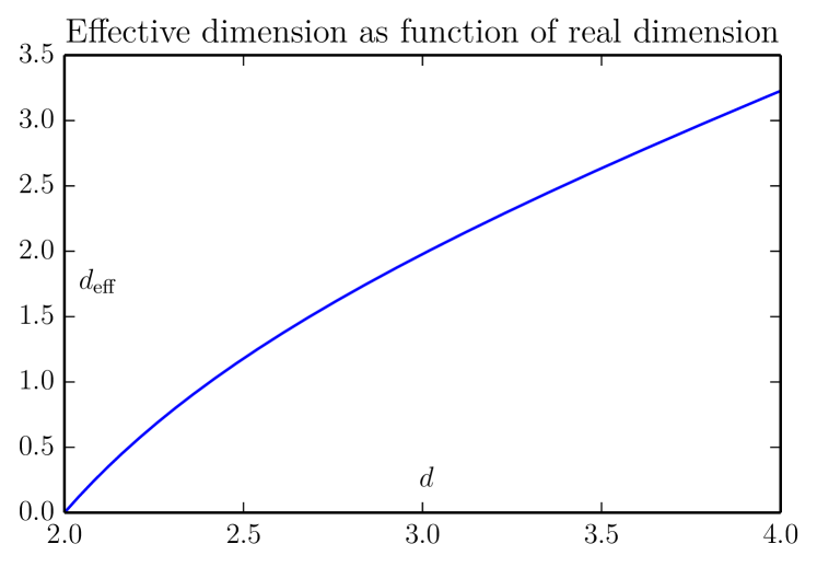
Figure 3: Effective dimension $d_{\text{eff}}=1/(2R)$ from the MSA solution that follows from the integral (52). Note that $R$ is independent of spin dimensionality.

Hence the MSA condition for the critical line becomes

$$R=\langle s^{2}\rangle=\frac{\int s^{2}f(s)\text{e}^{-c_{0}s^{2}/2}\ ds}{\int f(s)e^{-c_{0}s^{2}/2}\ ds}.$$ (48)

For multicomponent spins the $s$ becomes a vector $\mathbf{s}$, and the $R$ is replaced with $RN$, i.e. $R=\langle s_{1}^{2}\rangle$ ($N$ is spin dimension).

For the field theory considered in the mean field limit in section 6 we have the equivalent spin model with $s\rightarrow\varphi\rightarrow\bm{\varphi}$. The corresponding spin distribution is

$$f(\bm{\varphi})=e^{-\frac{1}{2}(m^{2}+2d)\bm{\varphi}^{2}-\frac{1}{4!}\lambda(\bm{\varphi}^{2})^{2}}$$ (49)

with nearest neighbor interaction such that

$$\beta\tilde{\psi}(\mathbf{0})=-2d.$$ (50)

When the inverse range of attraction $\gamma\rightarrow 0$ the mean field limit is obtained. In the limit the $\tilde{\psi}(\mathbf{k})$ will approach zero except for a peak of width $\propto\gamma$ around $\mathbf{k}=0$. Thus in the limit $\gamma\rightarrow 0$ the $\tilde{\psi}(\mathbf{k})$ will no longer contribute to the core condition integral (26) by which the parameter $c_{0}$ will be zero. Thus the effective spin distribution (30) will be the given one eq. (49). With eqs. (25) and (50) this at the critical point implies

$$R=\frac{1}{2d}.$$ (51)

Altogether, with $NR=\int\bm{\varphi}^{2}f(\bm{\varphi})\ d\bm{\varphi}/\int f(\bm{\varphi})\ d\bm{\varphi}$, eq. (46) is recovered in the limit $\gamma\rightarrow 0$.

With finite $\gamma$, however, the $c_{0}$ will be non-zero, and the core condition integral can be written as

$$R =\frac{1}{(2\pi)^{d}}\int\frac{R_{e}\ d\mathbf{k}}{1-R_{e}(-\beta\tilde{\psi}(\mathbf{k}))}=\frac{1}{2d}\frac{1}{(2\pi)^{d}}\int\frac{d\mathbf{k}}{1-(-\beta\tilde{\phi}(\mathbf{k})/2d)},$$ (52)

with $R_{e}=R/(1-Rc_{0})$ where $R_{e}=1/(2d)$ at the critical point. From this one finds $c_{0}=R^{-1}-R_{e}^{-1}=R^{-1}-2d$. With (30) this means that the effective spin distribution becomes expression (49) with $2d$ replaced by $R^{-1}$. Hence the MSA condition for the critical line becomes

$$\text{Tr}\,\mathbf{G}^{(0)}(\bm{0})=NR=\frac{\int\bm{\varphi}^{2}\,\text{e}^{-\frac{1}{2}\left(m^{2}+R^{-1}\right)\,\bm{\varphi}^{2}-\frac{1}{4!}\lambda(\bm{\varphi}^{2})^{2}}\,\text{d}\bm{\varphi}}{\int\text{e}^{-\frac{1}{2}\left(m^{2}+R^{-1}\right)\,\bm{\varphi}^{2}-\frac{1}{4!}\lambda\,(\bm{\varphi}^{2})^{2}}\text{d}\bm{\varphi}}.$$ (53)

This is just the mean field condition (46) with $(2d)^{-1}$ replaced by $R=\int_{0}^{\infty}\text{e}^{-2dt}\,I_{0}(2t)^{d}\,dt$ which follows when eqs. (67) and (68) for nearest neighbor interaction are applied to eq. (52). Altogether, as far as the critical line is concerned, the MSA method is equivalent to mean field theory in an effective dimension $d_{\text{eff}}=\frac{1}{2}R^{-1}$ (independent of $N$), as plotted in figure 3.

Series solutions of eq. (53) with respect to $m^{2}$ can be found for small and large values of $\lambda$, and are given in the following sections.

7.1 Small-$\lambda$ expansion of the MSA solution

For small $\lambda$ we find, cf. appendix D.1,

$$Rm^{2}= -(N+2){\textstyle\big{(}\frac{R^{2}\lambda}{6}\big{)}}+2(N+2)\left[{\textstyle\big{(}\frac{R^{2}\lambda}{6}\big{)}^{2}}-(N+8){\textstyle\big{(}\frac{R^{2}\lambda}{6}\big{)}^{3}}\right.$$

$$+(N^{2}+26N+108){\textstyle\big{(}\frac{R^{2}\lambda}{6}\big{)}^{4}}-(N^{3}+58N^{2}+684N+1\,984){\textstyle\big{(}\frac{R^{2}\lambda}{6}\big{)}^{5}}$$ (54)

$$+\left.(N^{4}+108N^{3}+2\,584N^{2}+19\,824N+45\,280){\textstyle\big{(}\frac{R^{2}\lambda}{6}\big{)}^{6}}+\cdots\right].$$

This expansion has the same form as eq. (44), but with no sum over lattice points (i.e. like a zero-dimensional model), with the propagator replaced by the constant $R=a_{1}$. Hence, the MSA reproduces first order of perturbation theory exactly. It further predicts a magnitude of the second order term ($a_{2}$) which is about 8% too small, and of the third order term which (for $N=1$) is about 20% too small.

7.2 Large-$\lambda$ expansion of the MSA solution

For large $\lambda$ we find, cf. appendix D.2,

$$NRm^{2}= -{\textstyle\frac{N^{2}R^{2}\lambda}{6}}-2+2(N-2)\left[{\textstyle\big{(}\frac{6}{N^{2}R^{2}\lambda}\big{)}}-(N-8){\textstyle\big{(}\frac{6}{N^{2}R^{2}\lambda}\big{)}^{2}}\right.$$

$$+(N^{2}-26N+108){\textstyle\big{(}\frac{6}{N^{2}R^{2}\lambda}\big{)}^{3}}-(N^{3}-58N^{2}+684N-1\,984){\textstyle\big{(}\frac{6}{N^{2}R^{2}\lambda}\big{)}^{4}}$$ (55)

$$+\left.(N^{4}-108N^{3}+2\,584N^{2}-19\,824N+45\,280){\textstyle\big{(}\frac{6}{N^{2}R^{2}\lambda}\big{)}^{5}}+\cdots\right].$$

This expression may seem to indicate an exact result for $N=2$. This is not the case; we see from eq. (71) that there are contributions which vanishes exponentially fast as $\lambda\to\infty$. Such terms contributes to the small-$\lambda$ perturbation expansion in eq. (54). I.e., the large-$\lambda$ expansion to all orders — even if it could be summed to an exact expression — may not reproduce the small-$\lambda$ behavior (and vice versa). In reality, the expansion constitutes only an asymptotic series, in which case it becomes an interesting question whether the infinite set of expansion coefficients contain sufficient information to reproduce the exact result.

Surprisingly, a comparison of eqs. (54) and (55) reveals that the coefficients of the large-$\lambda$ expansion, except the leading one, are intriguingly related to the coefficients of the small-$\lambda$ expansion. Specifically, for the terms inside the brackets, by the relations

$$\big{(}{\textstyle\frac{6}{N^{2}R^{2}\lambda}}\big{)}^{k} \rightarrow(-1)^{k+1}\big{(}\textstyle{\frac{R^{2}\lambda}{6}}\big{)}^{k+1},$$ (56a)

$$N \rightarrow-N,$$ (56b)

for $k=1,2,\ldots$. We have not uncovered the origin of this duality relation; it is reason to expect that it is related to a Hubbard-Stratanovich transformation of the integrals in eq. (53).

The Ising limit is obtained as $\lambda\to\infty$, with $m^{2}=-\frac{1}{6}R\lambda$ on the critical line. We introduce a new variable $s=\varphi/\sqrt{R}$ to impose the Ising spin condition, $s^{2}=1$. This scaling introduces a temperature parameter $\beta=R$ in the interaction term. Hence the MSA predicts a critical temperature $\beta_{c}=R=0.154\,933\ldots$ for the $4d$ Ising model. This model has been investigated by Gaunt, Sykes and McKenzie GauntSykesMcKenzie79 using series expansion methods, and more recently by Lundow and Markström LundowMarkstrom09 using Monte-Carlo simulations, indicating a critical temperatature of $\beta_{c}=0.149\,694\,7\pm 5\cdot 10^{-7}$. I.e., the MSA prediction is only $3.5\%$ too large in the Ising limit. Since the MSA is exact to first order in $\lambda$, and also becomes exact in the limit $N\to\infty$, the Ising limit ($\lambda\to\infty$, $N=1$) is probably the most inaccurate case of the models we have analyzed, since it is the opposite of these exact limits.

With SCOZA, where thermodynamic self-consistency is imposed, accuracy is expected to increase further, as discussed a bit at the end of section 3.2.

7.3 $1/N$-expansion of the MSA solution

We introduce $u=\frac{1}{6}N{R}^{2}\,\lambda$ and consider the limit where $N$ becomes large with $u$ fixed. This defines a $1/N$-expansion, cf. appendix D.3,

$$R\,m^{2}= -u+\sum_{k\geq 1}c_{k}(u)\,N^{-k}$$

$$= -u-\frac{1}{1+u}\,{\left(\frac{2u}{N}\right)}+\frac{(1-u)}{(1+u)^{4}}\,{\left(\frac{2u}{N}\right)^{2}}-\frac{4(1-3u+u^{2})}{(1+u)^{7}}\,{\left(\frac{2u}{N}\right)^{3}}$$

$$+\frac{(1-u)(27-122u+27u^{2})}{(1+u)^{10}}\,{\left(\frac{2u}{N}\right)^{4}}$$ (57)

$$-\frac{4\,(62-521u+990u^{2}-521u^{3}+62u^{4})}{(1+u)^{13}}\,{\left(\frac{2u}{N}\right)^{5}}+\cdots$$

A further expansion of this expression in powers of $u$ agrees with a $1/N$-expansion of eq. (54). A further expansion of this expression in powers of $u^{-1}$ agrees with the $1/N$-expansion of eq. (55). But also the expansion (57) is inexact, since we leave out exponentially small (in $N-2$) contributions to the integrals in eq. (74). Note again the curious $u\to 1/u$ (anti-)symmetry of the coefficient functions present in eq. (57), which is revealed explicitly in figure 4.

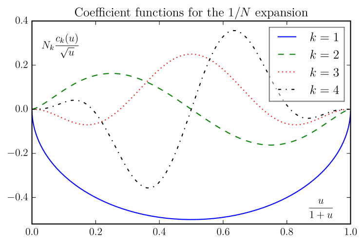
Figure 4: The first few coefficient functions of the $1/N$-expansion (57). The parameter $x\equiv u/(1+u)$ used on the $x$-axis maps to $1-x$ when $u\to 1/u$. The quantities $c_{k}(u)/\sqrt{u}$ used on the $y$-axis maps to $(-1)^{k-1}\,c_{k}(u)/\sqrt{u}$. The constant $N_{k}$ equals $\frac{1}{2}$ for $k=1$, otherwise 1.

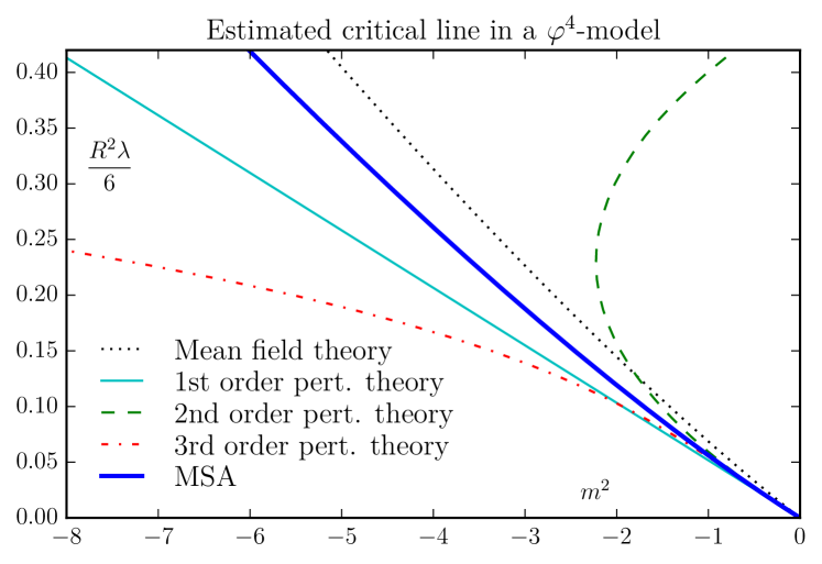
Figure 5: Some predictions of the critical line in the 4-dimensional $\varphi^{4}$-model (for $N=1$). The mean field result is inaccurate already to first order in $\lambda$. Visually, the MSA prediction is almost indistinguishable from the perturbation expansion in the region where the latter looks trustable. To better expose the differences we present the same results in a different way in figure 6.

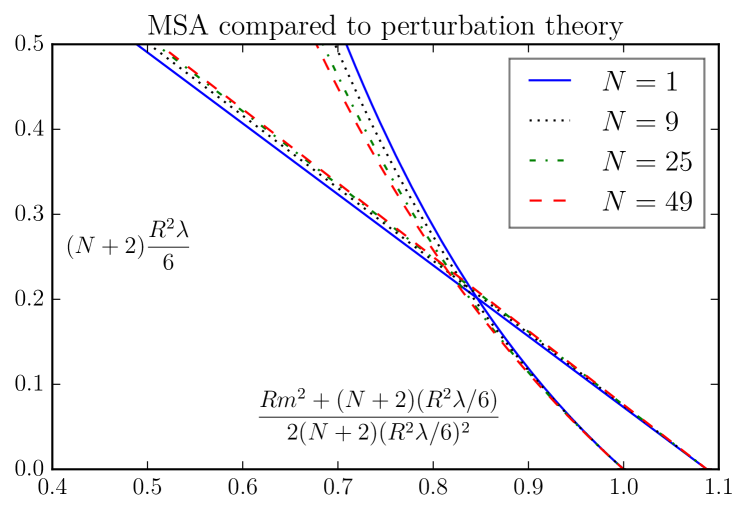
Figure 6: Detailed view of the small $\lambda$ behaviour of the critical line. To better expose the differences we have subtracted the exact first order term from $Rm^{2}$, and further scaled the axes. Thus, the $\lambda^{3}$-term of the exact perturbation expansion (44) becomes a straight line. It shows a weak dependence of the spin dimensionality $N$ beacuse the third order diagrams in figure 2 are proportional to both $(N+2)^{2}$ and $(N+2)(N+8)$, cf. (44b). The curved lines represent the MSA solution starting at position $1.0$ for $\lambda=0$ (by construction). The offset in starting point relative to the perturbative straight line is due to an 8 % error in the MSA prediction of the $\lambda^{2}$-behaviour; the differerence in the starting slope is due to a 20 % error in the MSA prediction of the $\lambda^{3}$-behaviour, cf. eq. (54).

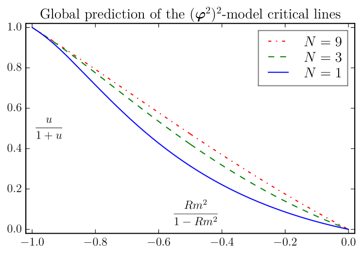
Figure 7: A global view of the the MSA prediction for the critical line. To cover the full range of interaction strengths a non-linear parametrization of axes is used, with $u=\frac{1}{6}NR^{2}\lambda$. The critical line is linear in $\lambda$ for both very small and very large $\lambda$, behaving respectively like $Rm^{2}=-\frac{1}{6}(N+2)R^{2}\lambda+\mathcal{O}(\lambda^{2})$ and $Rm^{2}=-\frac{1}{6}NR^{2}\lambda-2/N+\mathcal{O}(\lambda^{-1})$, cf. eqs. (54) and (55). The small-$\lambda$ behaviour is exact, the large-$\lambda$ behaviour is about 3 % too high (for $\bm{\varphi}$-dimension $N=1$ and space-time dimension $d=4$). This is expected to become more accurate as $N$ increases.

8 Numerical computations

The integrals in eqs. (46) and (53) can be transformed to standardized integrals, like $\mathcal{K}_{2n}(x)$ defined by (79) when $m^{2}+2d_{\text{eff}}>0$, and $\mathcal{I}_{2n}(x)$ defined by (80) when $m^{2}+2d_{\text{eff}}<0$. For the mean field case, eq. (46), $d_{\text{eff}}\to d$. The $\mathcal{K}_{2n}(x)$ and $\mathcal{I}_{2n}(x)$ when $n$ is non-negative integer, can be expressed in terms of modified Bessel functions of order $\frac{1}{4}$ and $\frac{3}{4}$, and more elementary functions, cf. appendix D.4.

In terms of these functions the exact mean field and MSA solutions for the critical line can be written in parametric form

$$\begin{split}\lambda&=6\left[\frac{2}{NR}\frac{\mathcal{K}_{2(n+1)}(x)}{\mathcal{K}_{2n}(x)}\right]^{2},\\ m^{2}&=-1/(NR)+\sqrt{\lambda/6}\,x,\end{split}$$ (58a)

with $$0<x<\infty N=2n+1 m^{2}+(1/R)>0 m^{2}\to 0^{-} x\to\infty m^{2}+(1/R)<0$$. The spin dimensionality is . This covers the region , where when . The region is covered by the parametrization

$$\begin{split}\lambda&=6\left[\frac{2}{NR}\frac{\mathcal{I}_{2(n+1)}(y)}{\mathcal{I}_{2n}(y)}\right]^{2},\\ m^{2}&=-1/(NR)-\sqrt{\lambda/6}\,y,\end{split}$$ (58b)

with $$0<y<\infty m^{2}\to-\infty y\to\infty$$, where when .

The $K_{2n}$ and $I_{2n}$ are integrals given by eqs. (79) and (80) in appendix D.4.

A global view of the resulting critical lines is given in figure 7 where non-linear quantities in terms of $\lambda$ and $m^{2}$ are used. In figure 5 comparison with perturbation theory has been performed ($N=1$), and in figure 6 this has been performed in more detail.

With a linear scale in terms of $\lambda$ and $m^{2}$ the qualitative behavior of the global phase diagram follows in an obvious way from the term linear in each of eqs. (54) and (55) and the constant term in the latter. The slopes of the straight lines formed by these terms, will be the same in the limit $N\rightarrow\infty$ by which they join in just one straight line. If the $N\rightarrow\infty$ curve had been drawn on figure  7, it would also be a straight line there. For finite $N$ these two straight lines will intersect at $-m^{2}=(N+2)/(NR)$ (where $R=a_{1}=0.154933\cdots$). Thus at this position the critical line will have an intermediate slope. So altogether the critical line starts with one slope at $\lambda=0$. Then the magnitude of this slope increases somewhat in a monotonic way towards its large $\lambda$ value (with $m^{2}$ on the horizontal axis). In view of the simplicity of this situation we have not drawn separate figures for these slightly bent lines.

Appendix A Gaussian model with finite temperature and chemical potential

Consider the gaussian path integral

$$\Xi=\int\text{e}^{-\int dt\,\left[(\partial_{t}-\bar{\mu}){\varphi}^{*}(\partial_{t}+\bar{\mu}){\varphi}+\bar{\varepsilon}^{2}\varphi^{*}\varphi\right]}\,\mathcal{D}\varphi^{*}\mathcal{D}\varphi,$$ (59)

where $\mu\equiv\hbar\bar{\mu}$ is a chemical potential, and $\varepsilon\equiv\hbar\bar{\varepsilon}$ a site energy. The integration is over all complex continuous functions $\varphi(t)$ defined on a circle of circumference $\tau=\hbar\beta$. Expand $\varphi(t)$ in a Fourier series, $\varphi(t)=\sum_{n}\varphi_{n}\,\text{e}^{-\text{i}\omega_{n}t}$, with Matsubara frequencies $\omega_{n}=2\pi n/\tau$. Define further the integration measure as $\mathcal{D}\varphi^{*}\mathcal{D}\varphi=\tau^{-2}d\varphi^{*}_{0}d\varphi_{0}\prod_{n\neq 0}\omega_{n}^{2}d\varphi^{*}_{n}d\varphi_{n}$, where each complex Fourier coefficient is integrated over the complex plane (normalized such that $\int\text{e}^{-z^{*}z}\,dz^{*}dz=1$). This gives

$$\Xi =\int\text{e}^{-(\bar{\varepsilon}^{2}-\bar{\mu}^{2})\varphi_{0}^{*}\varphi_{0}}\,\tau^{-2}d\varphi_{0}^{*}d\varphi_{0}\prod_{n\neq 0}\omega_{n}^{2}\;\int\,\text{e}^{-\left[(\omega_{n}+\text{i}\bar{\mu})^{2}+{\bar{\varepsilon}}^{2}\right]\varphi^{*}_{n}\varphi_{n}}d\varphi^{*}_{n}d\varphi_{n}$$

$$=\frac{(k_{\text{B}}T)^{2}}{{\varepsilon}^{2}-{\mu}^{2}}\prod_{n\neq 0}{\left(1+\frac{2\text{i}\bar{\mu}}{\omega_{n}}+\frac{\bar{\varepsilon}^{2}-\bar{\mu}^{2}}{\omega^{2}_{n}}\right)^{-1}}=\frac{\text{e}^{-\beta{\varepsilon}/2}}{1-\text{e}^{-\beta({\varepsilon}-{\mu})}}\,\frac{\text{e}^{-{\beta\varepsilon}/2}}{1-\text{e}^{-\beta({\varepsilon}+{\mu})}}.$$ (60)

The last equality follows (after some work) from the relation $\prod_{n=1}^{\infty}(1+z^{2}/n^{2})=\sinh\pi z/\pi z$. This demonstrates that the path integral (59) defines the grand canonical partition function for non-interacting bosons (particles and antiparticles) occupying a quantum dot at temperature $T$. There is a zero-point energy $\frac{1}{2}\varepsilon$ per particle type, a site occupation energy $\varepsilon$, and a chemical potential $\mu$ for particles and $-\mu$ for antiparticles. It should be clear that this connenection can be extended to arbitrary many harmonic oscillators, and — by including factors like $\text{exp}\left[\int dt\,\varphi^{*}(t)h(t)+h^{*}(t)\varphi(t)\right]$ — to the corresponding generating functions.

Appendix B MSA solution of gaussian model

The partition function of the gaussian model can also be found by using the lattice gas picture of a mixture of particles. Again we will use the MSA. With pressure $p$ we have with eq. (10b)

$$\beta p=I+\sum_{s}\beta\mu_{s}\rho_{s}.$$ (61)

With eqs. (18) and (22)

$$I=I_{R}+\frac{1}{2}{\,\texttt{m}}^{2}\tilde{v}(0)+I_{1}.$$ (62)

Further from eq. (29) one has the effective chemical potentials for the reference system (the ones that give the resulting densities $\rho_{s}$)

$$\beta\mu_{es}=\ln z_{es}=\ln f_{e}(s)+\beta{\cal H}_{e}s.$$ (63)

Now with eqs. (14b), (30), (36), and (38) the reference system (free spins) pressure is

$$\beta p_{R}=I_{R}+\sum_{s}\beta\mu_{es}\rho_{s}=\ln\rho_{0}=\frac{1}{2}\ln R+\frac{1}{2}\beta{\cal H}_{e}{\,\texttt{m}}$$ (64)

in accordance with eq. (13). Finally with eqs. (9) and (63) one has

$$\begin{split}\Delta I&=\sum_{s}(\beta\mu_{s}\rho_{s}-\beta\mu_{es}\rho_{s})\\ &=\sum_{s}\left(\frac{1}{2}c_{0}s^{2}-\tilde{v}(\mathbf{0}){\,\texttt{m}}s\right)\rho_{s}=\frac{1}{2}c_{0}(R+{\,\texttt{m}}^{2})-{\,\texttt{m}}^{2}\tilde{v}(\mathbf{0}),\end{split}$$ (65)

when eqs. (16a) and (16c) are used. Adding together we find

$$\begin{split}\beta p&=\beta p_{R}+\Delta I+\frac{1}{2}{\,\texttt{m}}^{2}\tilde{v}(\mathbf{0})+I_{1}\\ &=\frac{1}{2}\ln R-\frac{1}{2(2\pi)^{d}}\int_{-\pi}^{\pi}\cdots\int_{-\pi}^{\pi}\,\ln[1-R\tilde{v}(\mathbf{0})]\,d\mathbf{k}+\frac{1}{2}\beta\mathcal{H}{\,\texttt{m}},\end{split}$$ (66)

when (30) for $\beta{\cal H}_{e}$ is inserted. With $R^{-1}=R_{0}^{-1}+c_{0}$, and

$$\beta{\cal H}=\beta{\cal H}_{e}-\tilde{v}(\mathbf{0}){\,\texttt{m}}=[R^{-1}-\tilde{v}(0)]{\,\texttt{m}},\quad\text{where }\tilde{v}(\mathbf{0})=c_{0}-\beta\tilde{\psi}(\mathbf{0}),$$

this gives precisely the gaussian model result (34a).

Appendix C Integral representation of the lattice propagator

We want to evaluate integrals of the form

$$G(\bm{x};m^{2},\nu)\equiv\frac{1}{V_{\text{BZ}}}\int_{\text{BZ}}\frac{\text{e}^{\text{i}\bm{k}\cdot\bm{x}}}{\left(m^{2}+2d-\sum_{n=1}^{d}\cos k_{n}\right)^{\nu}}\,d\bm{k},$$ (67)

where the integral is over the Brillouin zone BZ of a $d$-dimensional hypercubic lattice, with volume $V_{\text{BZ}}$. The lattice propagator is obtained for $\nu=1$. By use of the formula $\int_{0}^{\infty}dt\,t^{\nu-1}\,\text{e}^{-at}=\Gamma(\nu)\,a^{-\nu}$ this can be rewritten as

$$G(\bm{x};m^{2},\nu) =\frac{1}{\Gamma(\nu)}\int_{0}^{\infty}\frac{dt}{t}\,t^{\nu}\,\text{e}^{-m^{2}t}\prod_{n=1}^{d}e^{-2t}\,\int_{-\pi}^{\pi}\frac{dk_{n}}{2\pi}\,\text{e}^{2t\cos k_{n}}\text{e}^{\text{i}k_{n}x_{n}}$$

$$=\frac{1}{\Gamma(\nu)}\int_{0}^{\infty}\frac{dt}{t}\,t^{\nu}\,\text{e}^{-m^{2}t}\,\prod_{n=1}^{d}\text{e}^{-2t}I_{x_{n}}(2t),$$ (68)

where $I_{n}(t)$ is a modified Bessel function.

Appendix D Evaluation of integrals and solution of the closure relation

The results presented in sections 7 and 8 requires evaluation of $\langle\bm{\varphi}^{2}\rangle$. In this appendix we give some details of how it can be evaluated in various parameter ranges, and how the closure relation

$$NR=\langle\bm{\varphi}^{2}\rangle$$ (69)

can be solved. A useful starting point is the formula

$$\langle\bm{\varphi}^{2}\rangle=\frac{d}{da}\ln\int\bm{e}^{a\bm{\varphi}^{2}-\frac{1}{4!}\lambda(\bm{\varphi}^{2})^{2}}d\bm{\varphi}\equiv\frac{d}{da}\ln Z,$$ (70)

where $a=-\frac{1}{2}(m^{2}+R^{-1})$. The algebraic manipulations can be performed by computer algebra, and verified against low order manual calculations.

D.1 Perturbation expansion for small $\lambda$

We use the fact that $\frac{d}{da}\ln Z=2R^{2}\frac{d}{dR}\ln Z$ when $a=-\frac{1}{2}(m^{2}+R^{-1})$, and transform eq. (70) to the relation

$$\begin{split}\langle\bm{\varphi}^{2}\rangle&=NR\\ &+2R^{2}\frac{d}{dR}\ln\int_{0}^{\infty}t^{(N-2)/2}\,\text{e}^{-t}\,\text{e}^{-m^{2}Rt-\frac{1}{6}\lambda R^{2}t^{2}}dt,\end{split}$$

which is satisfied for $\lambda=0$ if we assume $m^{2}=0$ to $0^{\text{th}}$ order in $\lambda$. We thus make the ansatz that $m^{2}=\sum_{n=1}^{\infty}m^{2}_{n}\lambda^{n}$, expand the integral and its logarithm in powers of $\lambda$, and insert this expansion into eq. (69). The resulting equation can now be solved recursively for the coefficients $m^{2}_{n},\;n=1,2,\ldots$. The first terms of this expansion are given in eq. (54).

D.2 Asymptotic expansion for large $\lambda$

A first estimate of the integral in eq. (70) by the Laplace method gives $\ln Z\approx 6a^{2}/\lambda$, implying that $a\approx\frac{1}{12}NR\lambda$ for large $\lambda$. Hence the parameter $v\equiv NR\lambda/(12a)$ is close to 1 in this limit, with a deviation which can be expanded in the small quantity $\epsilon\equiv 1/(NRa)$. With

$$\varepsilon\equiv\sqrt{{\lambda}/{12}}\,a^{-1}=\sqrt{v\,\epsilon},$$

eq. (70) can be transformed to the form

$$\begin{split}v&=1+\text{$\frac{1}{2}$}(N-2)v\epsilon\\ &-v\epsilon\Big{[}\varepsilon\frac{d}{d\varepsilon}\int^{\infty}_{-1/\varepsilon}(1+\varepsilon\,t)^{(N-2)/2}\,\text{e}^{-\frac{1}{2}t^{2}}dt\Big{]}_{\varepsilon^{2}=v\epsilon}.\end{split}$$ (71)

An asymptotic expansion of the integral as $\varepsilon\to 0^{+}$ is straightforward to generate by binomial expansion and term-by-term integration. eq. (71) may next be solved as an expansion, $v=1+\sum_{n\geq 1}v_{n}\,\epsilon^{n}$, such that one finds (from the definition of $v\equiv\epsilon/\delta$),

$${12}/(N^{2}R^{2}\lambda)\equiv\delta=\epsilon\,\Big{(}1+\sum_{n\geq 1}v_{n}\epsilon^{n}\Big{)}^{-1}.$$ (72)

This relation can be inverted to an expansion $\epsilon=\delta\,(1+\sum_{n\geq 1}\epsilon_{n}\delta^{n})$. It finally follows that

$$NRm^{2}=-N-(2/\delta)\Big{(}1+\sum_{n\geq 1}\epsilon_{n}\delta^{n}\Big{)}^{-1}.$$ (73)

The first few terms of this expansion are given in eq. (55).

D.3 Asymptotic expansion for large $N$

Eq. (53) can be written as

$$\tilde{R}=\frac{\int_{0}^{\infty}\rho\,\text{e}^{\frac{1}{2}(N-2)\left[\ln\rho+2a\rho-\frac{1}{2}\tilde{u}\rho^{2}\right]}d\rho}{\int_{0}^{\infty}\text{e}^{\frac{1}{2}(N-2)\left[\ln\rho+2a\rho-\frac{1}{2}\tilde{u}\rho^{2}\right]}d\rho}\equiv\langle\rho\rangle,$$ (74)

where we have introduced $\rho=\bm{\varphi}^{2}/(N-2)$, $\tilde{R}=NR/(N-2)$, and $\tilde{u}=\frac{1}{6}(N-2)\lambda$. When $(N-2)$ is large the main contribution to the integrals comes from the vicinity of the maximum point $\rho_{0}$, satisfying

$$a=-\frac{1}{2}\left(\rho_{0}^{-1}-\tilde{u}\rho_{0}\right).$$ (75)

Hence, to leading order in $N$ eq. (74) becomes $\tilde{R}=\langle\rho\rangle=\rho_{0}$. I.e.,

$$\begin{split}a&\equiv-\frac{1}{2}\left(m^{2}+R^{-1}\right)=-\frac{1}{2}\left(\tilde{R}^{-1}-\tilde{u}\,\tilde{R}\right),\\ &\text{or}\quad m^{2}=-\tilde{u}\,\tilde{R}=-\frac{1}{6}NR\lambda,\end{split}$$

since $\tilde{R}=R$ to leading order. To proceed we expand the integrals in (74) in powers of $\bar{\nu}\equiv 1/(N-2)$. By introducing $\bar{v}\equiv\rho_{0}^{2}\,\tilde{u}=\frac{1}{6}(N-2)\rho_{0}^{2}\,\lambda$, eq. (74) acquires the form

$$\tilde{R}=\rho_{0}\,\Big{[}1+\sum_{k\geq 1}r_{k}(\bar{v})\;\bar{\nu}^{k}\Big{]},$$ (76)

where the coefficients $r_{k}$ are rational functions in $\bar{v}$. Eq. (76) can be viewed as an equation for $\rho_{0}$, or equivalently for $\bar{v}$. We solve it by introducing $\bar{u}\equiv\tilde{R}^{2}\,\tilde{u}$, such that $\tilde{R}/\rho_{0}=\sqrt{\bar{u}/\bar{v}}$. Then eq. (76) may be rewritten as

$$\bar{u}=\bar{v}\,\Big{[}1+\sum_{k\geq 1}r_{k}(\bar{v})\;\bar{\nu}^{k}\Big{]}^{2},$$ (77)

and solved iteratively for $\bar{v}$ order by order in $\bar{\nu}$, leading to $\bar{v}=\bar{u}(1+\sum_{k\geq 1}s_{k}(\bar{u})\,\bar{\nu}^{k})$. Finally, using (75), the expression for the critical line can be expressed as

$$\tilde{R}\,m^{2}=-\tilde{R}R^{-1}+\sqrt{\bar{u}/\bar{v}}-\sqrt{\bar{u}\bar{v}}.$$ (78)

With the expansion for $\bar{v}$ known, this is straightforward to expand once more. Finally, for simpler comparison with the expressions for small and large $\lambda$, we rewrite the expression as an expansion in $\nu\equiv 1/N=\bar{\nu}/(1+2\bar{\nu})$ and $u\equiv\frac{1}{6}NR^{2}\lambda=\bar{u}/(1+2\bar{\nu})$. The first terms of this expansion are given in eq. (57).

D.4 Exact expressions

The integrals in eq. (46) can be evaluated exactly. The results involve different functions depending on whether $N$ is even or odd. We will here only discuss the more complicated cases when $N=2n+1$ is odd. By introducing a new variable of integration, $t^{4}=\lambda(\bm{\varphi}^{2})^{2}/4!$, the relevant integrals can be transformed the form

$$\mathcal{K}_{2n}(u)\equiv 2\int_{0}^{\infty}t^{2n}\,\text{e}^{-t^{4}-u\,t^{2}}dt,$$ (79)

and the corresponding expression with $u$ replaced by $-v$,

$$\mathcal{I}_{2n}(v)\equiv 2\int_{0}^{\infty}t^{2n}\,\text{e}^{-t^{4}+v\,t^{2}}dt.$$ (80)

The integral (79) can be found in the integral table GradshteynRyzhik81 for $n=0$. Then higher values of $n$ by can be derived by repeated differentation with respect to $u$. The corresponding integrals (80) can next be found by analytic continuation, $u\to u\,\text{e}^{\text{i}\phi}$ with $0\leq\phi\leq\pi$. Introduce

$$\begin{split}f(u)&\equiv u^{1/2}\,\text{e}^{\frac{1}{8}u^{2}}\,K_{1/4}({\textstyle\frac{1}{8}}u^{2}),\\ g(u)&\equiv u^{3/2}\,\text{e}^{\frac{1}{8}u^{2}}\,K_{3/4}({\textstyle\frac{1}{8}}u^{2}).\end{split}$$ (81)

We find that $\mathcal{K}_{0}(u)=\frac{1}{2}f(u)$. From the recursion relations for Bessel functions AbramowitzStegun , specifically $K^{\prime}_{1/4}(z)=-\frac{1}{4z}K_{1/4}(z)-K_{3/4}(z)$ and $K^{\prime}_{3/4}(z)=-K_{1/4}(z)-\frac{3}{4z}K_{3/4}(z)$, it next follows that

$$\frac{d}{du}\begin{pmatrix}f(u)\\ g(u)\end{pmatrix}=\frac{1}{4}\begin{pmatrix}u&-1\\ -u^{2}&u\end{pmatrix}\begin{pmatrix}f(u)\\ g(u)\end{pmatrix}.$$ (82)

Hence we may write

$$\mathcal{K}_{2n}(u)=P_{n}(u)f(u)+Q_{n}(u)g(u),$$ (83)

where $P_{n}$ and $Q_{n}$ are polynomials in $u$, satisfying the recursion relation

$$\begin{pmatrix}P_{n+1}(u)\\ Q_{n+1}(u)\end{pmatrix}=-\frac{d}{du}\begin{pmatrix}P_{n}(u)\\ Q_{n}(u)\end{pmatrix}-\frac{1}{4}\begin{pmatrix}u&-u^{2}\\ -1&u\end{pmatrix}\begin{pmatrix}P_{n}(u)\\ Q_{n}(u)\end{pmatrix},$$ (84)

starting with $P_{0}=\frac{1}{2}$, $Q_{0}=0$. The next few polynomials are listed in table 1. Analytic continuation leads to the representation

$n$	$(-)^{n}\,2^{n+2}\,P_{n}$	$(-)^{n+1}\,2^{n+2}\,Q_{n}$
$0$	$2$	$0$
$1$	$u$	$1$
$2$	$u^{2}+2$	$u$
$3$	$u^{3}+5u$	$u^{2}+3$
$4$	$u^{4}+10u^{2}+10$	$u^{3}+8u$
$5$	$u^{5}+17u^{3}+45u$	$u^{4}+15u^{2}+21$

Table 1: The first few polynomials $P_{n}$ and $Q_{n}$ in (83) and (85).

$$\mathcal{I}_{2n}(v)={P}_{n}(-v)\bar{f}(v)+{Q}_{n}(-v)\bar{g}(v),$$ (85)

where

$$\bar{f}(v) =v^{1/2}\text{e}^{\frac{1}{8}v^{2}}\left[K_{1/4}({\textstyle\frac{1}{8}}v^{2})+\sqrt{2}\,\pi I_{1/4}({\textstyle\frac{1}{8}}v^{2})\right],$$ (86a)

$$\bar{g}(v) =v^{3/2}\text{e}^{\frac{1}{8}v^{2}}\left[K_{3/4}({\textstyle\frac{1}{8}}v^{2})+\sqrt{2}\,\pi I_{3/4}({\textstyle\frac{1}{8}}v^{2})\right].$$ (86b)

The final analytic expressions have been checked (successfully) against direct numerical evaluation for a number of cases.

References

- (1) R. P. Feynman, Space-time approach to nonrelativistic quantum mechanics, Rev. Mod. Phys. 20 (1948) 367–387.
- (2) R. P. Feynman, Space - time approach to quantum electrodynamics, Phys. Rev. 76 (1949) 769–789.
- (3) R. P. Feynman and A. R. Hibbs, Quantum Mechanics and Path Integrals. McGraw-Hill, New York, 1965.
- (4) M. E. Peskin and D. V. Schroeder, An introduction to quantum field theory. Westview Press, Boulder, Colorado, 1995.
- (5) H. Kleinert and V. Schulte-Frohlinde, Critical Properties of Theories. World Scientific, 2001.
- (6) J. S. Høye and G. Stell, SCOZA for continuous spins, Phys.A 247 (1997) 497.
- (7) P. C. Hemmer, On the van der Waals Theory of the Vapor-Liquid Equilibrium. IV. The Pair Correlation Function and Equation of State for Long-Range Forces, J.Math.Phys. 5 (1964) 75.
- (8) J. L. Lebowitz, G. Stell and S. Baer, Separation of the Interaction Potential into Two Parts in Treating Many-Body Systems. I. General Theory and Applications to Simple Fluids with Short-Range and Long-Range Forces, J.Math.Phys. 6 (1965) 1282.
- (9) J. S. Høye and G. Stell, Thermodynamics of the MSA for simple fluids, J. Chem. Phys. 67 (1977) 439–445.
- (10) T. H. Berlin and M. Kac, The Spherical Model of a Ferromagnet, Phys. Rev. 86 (1952) 821.
- (11) H. W. Lewis and G. H. Wannier, Spherical Model of a Ferromagnet, Phys. Rev. 88 (1952) 682.
- (12) J. L. Lebowitz and J. K. Percus, Mean Spherical Model for Lattice Gases with Extended Hard Cores and Continuum Fluids, Phys. Rev. 144 (1966) 251.
- (13) J. Høye and G. Stell, Ornstein-Zernike equation for a two-Yukawa with core condition, Mol.Phys. 52 (1984) 1057.
- (14) J. Høye and G. Stell, Toward a liquid-state theory with accurate critical-region behavior, Int.J.Thermophys. 6 (1985) 561.
- (15) R. Dickman and G. Stell, Self-Consistent Ornstein-Zernike Approximation for Lattice Gases, Phys. Rev. Lett. 77 (1996) 996.
- (16) J. S. Høye and A. Borge, Self consistent Ornstein-Zernike approximation compared with exact results for lattice gases in one and two dimensions, J.Chem.Phys. 108 (1998) 8830.
- (17) J. S. Høye and E. Lomba, Analysis of the critical region of the hierarchical reference theory, Mol. Phys. 109 (2011) 2773.
- (18) E. Lomba and J. S. Høye, Critical region of dimensional spins: extension and analysis of the hierarchical reference theory, Mol.Phys. 112 (2014) 2892, [1311.2864].
- (19) A. Parola and L. Reatto, Recent developments of the hierarchical reference theory of fluids and its relation to the renormalization group, Mol.Phys. 110 (2012) 2859, [1202.1981].
- (20) M. E. Fisher and P. Pfeuty, Critical Behavior of the Anisotropic -Vector Model, Phys. Rev. B 6 (1972) 1889.
- (21) K. G. Wilson and J. Kogut, The renormalization group and the expansion, Phys. Rep. 12 C (1974) 75.
- (22) A. Parola and L. Reatto, Hierarchical reference theory of fluids and the critical point, Phys. Rev. A 31 (1985) 3309.
- (23) C. C. Yan and G. H. Wannier, Observations on the spherical model of a ferromagnet, J.Math.Phys. 6 (1965) 1833.
- (24) J. S. Høye and G. Stell, SCOZA for -dimensional spins, Phys. A 244 (1997) 176.
- (25) J. S. Høye and A. Reiner, Towards a unification of hierarchical reference theory and self-consistent Ornstein-Zernike approximation: Analysis of exactly solvable mean-spherical and generalized mean-spherical models, Phys. Rev. E 75 (2007) 041113.
- (26) D. S. Gaunt, M. F. Sykes and S. McKenzie, Susceptibility and fourth-field derivative of the spin- Ising model for and , J.Phys. A 12 (1979) 871.
- (27) P. H. Lundow and K. Markström, Critical behavior of the Ising model on the four-dimensional cubic lattice, Phys. Rev. E 80 (2009) 031104.
- (28) I. S. Grandshteyn and I. M. Ryzhik, Table of Integrals, Series, and Products. Corrected and Enlarged Edition. Academic Press, New York, 1981.
- (29) Abramowitz. M. and Stegun, I. A., Handbook of Mathematical Functions. Dover Publications, Inc., New York, 1972.