Rapid convergence for simulations that project from particles onto a fixed mesh

Abstract

The advantage of particle Lagrangian methods in computational fluid dynamics is that advection is accurately modeled. However, the calculation of space derivatives is complicated. On the other hand, Eulerian formulations benefit from a fixed mesh, but feature non-linear advection terms. It seems natural to combine these two, using particles to advect the information and a fixed mesh to calculate space derivatives. This idea goes back to Particle-in-Cell methods, and is here considered within the context of the finite element (FE) method for the fixed mesh, and the particle-FEM (pFEM) for the particles. A “projection” method is required to transfer field values from particles to mesh and vice versa — in this work simple interpolation is used. Our results confirm that projection errors, especially from particles to mesh, cause a slow convergence of the method if standard, linear, FEs, are employed — but also that the convergence rate is restored to values comparable to Lagrangian simulations if quadratically consistent shape functions for the particles are used. The same applies to computational resources, making projection a viable alternative to Lagrangian simulations. The procedure is validated on Zalesak’s disk problem, the Taylor-Green vortex sheet flow, and the Rayleigh-Taylor instability.

1 Introduction

In Lagrangian particle methods of computational fluid dynamics, advection is modelled by moving the particles along the velocity field. The equations of motion are free of explicit advective terms, which would in general require a special treatment [1]. On the other hand, the initial particle setup can become highly distorted, which can lead to a degradation of the quality of the space discretization. An Eulerian method, on the other hand, benefits from the setup being defined once, at the beginning of the calculation, usually on a prescribed mesh. The equations of motion, on the other hand, contain non-linear advection terms, and the resulting computational problems are likewise not so well posed. It therefore seems natural to combine the two approaches, using particles to advect the field information with time, and keeping the static mesh to compute space derivatives. This idea is not new, as it goes back to Particle-in-Cell methods [2, 3]. In the context of SPH similar methods have been presented, beginning at least with the remeshing technique of [4], and particle splitting [5]. To be precise, these SPH works do not use an Eulerian mesh, but they do concern the problem of interpolating the field values at points different from the position of the particles, which is the crucial problem addressed below. There has been much recent effort trying to bring together Lagrangian and Eulerian simulations [6, 7].

In Fig. 1 we plot a sketch of this idea. The information of a field may be transferred from the nodes of a mesh onto the particles, or vice versa. A vector field (such as the velocity or the pressure gradient) is depicted, but the same idea applies to scalar fields, such as the pressure or the density. We will employ $H$ to refer to the fixed mesh spacing, and $h$ for the mean interparticle distance.

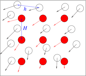
Figure 1: Main idea behind particle-in-cell methods. Fields (here, a vector field such as the velocity) are projected to and from the nodes of a fixed mesh (in red), with spacing $H$, onto particle nodes (in black), with mean spacing $h$.

In [8] this idea is explored, in the context of the finite element method (FEM) for the fixed mesh, and the particle FEM (pFEM) for the particles. We here follow these ideas, seeking to improve the errors associated with the interpolation (also referred to as projection) from particles to mesh and back. This source of error was identified, among others, as the one responsible for slow convergence of results. This finding is confirmed here, and we present a method that uses quadratically consistent interpolation from the particles to the mesh that leads to improved convergence. We want to remark that both that in those works and here, a simple interpolation procedure is used for projection. Other, more refined procedures may be studied, such as Galerkin projection, a technique developed to reduce the dimensionality of a problem in an optimal way [9, 10].

This article is structured as follows. The necessary theoretical background is laid out in Section 2, featuring a general introduction to integration errors and a discussion of shape functions. Results are presented in 3, for Zalesak’s disk (Section 3.1), the Taylor-Green vortex sheet (Section 3.2), and the Rayleigh-Taylor instability (Section 3.3). We end up with some conclusions in Section 5. The technical details concerning numerical methods and the procedure to obtain quadratic functions are given in the Appendices.

2 Theory

2.1 Integration errors

There are several sources of error associated to the spatial and temporal discretization of the continuous equations [8]. Let us write down a general equation for a field $A$ as

$$\frac{dA}{dt} =Q$$ (1)

$$\frac{d\mathbf{r}}{dt} =\mathbf{u}$$ (2)

where the time derivative is the convective derivative and $Q$ is a source term, which may include space derivatives of $A$. For a second-order integrator (such as the midpoint method) we will have, at each time iteration, an error appearing as

$$Ạ_{n+1}=Ạ_{n}+(\bar{Q}\pm\epsilon_{t})\Delta t,$$

where $\Delta t$ is the time-step, which we assume is fixed, $\bar{Q}$ is some mean value of the integrand, and the error is given by

$$\epsilon_{t}=\ddot{Q}\Delta t^{2}.$$

With $\ddot{Q}$ we refer to a quantity related to the second time derivative of $Q-\mathbf{u}\cdot\nabla A$. Its precise definition, and that of $\bar{Q}$, will change depending on the particular integration method and whether the simulation is Eulerian or Lagrangian [8]. (In the latter case, the convective term in $\ddot{Q}$ appears due to the errors in integrating the particles’ position, Eq. (2) ). These details do not concern us, since we focus on the dependence on $\Delta t$.

During a simulation with time span $T$, there will be $N_{t}=T/\Delta t$ steps, hence the total accumulated error due to time integration will be

$$E_{t}=N_{t}(\epsilon_{t}\Delta t)=\ddot{Q}T\Delta t^{2}.$$

For the error due to the linear spatial approximation of the FEM, a similar result is obtained, with an error

$$\epsilon_{x}=Q^{\prime\prime}\Delta x^{2},$$

where $\Delta x$ is the average distance between the nodes used to evaluate derivatives. Again, $Q^{\prime\prime}$ is a quantity related to the second space derivatives of $Q-\mathbf{u}\cdot\nabla A$. The total accumulated error will therefore be

$$E_{x}=N_{t}(\epsilon_{x}\Delta t)=Q^{\prime\prime}\Delta x^{2}T.$$

When increasing the resolution of a typical simulation, the value of $\Delta x$ is usually tied to $\Delta t$ by a prescribed Courant number

$$\mathrm{Co}:=\frac{u_{0}\Delta t}{\Delta x},$$

where $u_{0}$ is the maximum modulus of the velocity. The total error can then be written as

$$E=T\left(\ddot{Q}\Delta t^{2}+Q^{\prime\prime}\Delta x^{2}\right)=T\Delta t^{2}\left(\ddot{Q}+\frac{Q^{\prime\prime}u_{0}^{2}}{\mathrm{Co}^{2}}\right).$$

A convergence as $\Delta t^{2}$ is therefore expected for simple methods, including Eulerian methods and Lagrangian methods such as pFEM [11], and linearly consistent SPH [12].

If, on the other hand, the method involves a combination of a fixed mesh and particles, another source of error appears: the one due to projecting the fields from the mesh onto the particles and back. For the projection from the mesh onto the particles we expect

$$\epsilon_{\mathrm{mp}}=A^{\prime\prime}H^{2},$$ (3)

where the general $\Delta x$ is given by $H$, the mean mesh spacing (see Fig 1). At variance with the previous errors, this one is independent of the time spacing. The total accumulated error will be

$$E_{\mathrm{mp}}=A^{\prime\prime}H^{2}N_{t}=A^{\prime\prime}H^{2}\frac{T}{\Delta t}=A^{\prime\prime}T\frac{u_{0}^{2}}{\mathrm{Co}_{H}^{2}}\Delta t,$$ (4)

where in the last equality the mesh Courant number is introduced, as $\mathrm{Co}_{H}:=u_{0}\Delta t/H$. This error is seen to decrease only as $\Delta t$, compared with $\Delta t^{2}$ for straight pFEM.

Similarly, for the projection from the particles onto the mesh one expects

$$\epsilon_{\mathrm{mp}} =A^{\prime\prime}h^{2},$$ (5)

$$E_{\mathrm{pm}} =A^{\prime\prime}T\frac{u_{0}^{2}}{\mathrm{Co}_{h}^{2}}\Delta t,$$ (6)

where the particle Courant number is $\mathrm{Co}_{h}:=u_{0}\Delta t/h$, with the mean interparticle distance $h$ (see Fig 1). In Ref. [8] this source of error is minimized by introducing many particles, thus reducing $h$ and increasing $\mathrm{Co}_{h}$.

To summarize, the total error can be expected to be

$$E=T\left(\ddot{Q}\Delta t^{2}+Q^{\prime\prime}\Delta x^{2}+A^{\prime\prime}\frac{H^{2}}{\Delta t}+A^{\prime\prime}\frac{h^{2}}{\Delta t}\right),$$

where an ambiguous $\Delta x$ is kept, to be fixed as $H$ or $h$ depending on the simulation. In terms of the Courant numbers, one obtains

$$E=T\Delta t\left(\Delta t\left[\ddot{Q}+\frac{Q^{\prime\prime}u_{0}^{2}}{\mathrm{Co}^{2}}\right]+A^{\prime\prime}u_{0}^{2}\left[\frac{1}{\mathrm{Co}_{H}^{2}}+\frac{1}{\mathrm{Co}_{h}^{2}}\right]\right).$$

Moreover, the ratio $m:=h/H$ is usually fixed as the simulation is refined, resulting in a total error

$$E=T\Delta t\left(\Delta t\left[\ddot{Q}+\frac{Q^{\prime\prime}u_{0}^{2}}{\mathrm{Co}^{2}}\right]+A^{\prime\prime}\frac{u_{0}^{2}}{\mathrm{Co}_{h}^{2}}\left[1+\frac{1}{m^{2}}\right]\right),$$

which only decreases as $\Delta t$.

If, on the other hand, a quadratically consistent projection scheme from particles to mesh is used, we will have instead of Eqs. (3) and Eqs. (5),

$$\epsilon_{\mathrm{mp}}=A^{\prime\prime\prime}H^{3}\qquad\epsilon_{\mathrm{pm}}=A^{\prime\prime\prime}h^{3}.$$

We may then expect a total error

$$E=T\left(\ddot{Q}\Delta t^{2}+Q^{\prime\prime}\Delta x^{2}+A^{\prime\prime\prime}\frac{H^{2}}{\Delta t}+A^{\prime\prime\prime}\frac{h^{2}}{\Delta t}\right).$$

In terms of the Courant numbers,

$$E=T\Delta t^{2}\left(\ddot{Q}+\frac{Q^{\prime\prime}u_{0}^{2}}{\mathrm{Co}^{2}}+A^{\prime\prime\prime}u_{0}^{3}\left[\frac{1}{\mathrm{Co}_{H}^{3}}+\frac{1}{\mathrm{Co}_{h}^{3}}\right]\right),$$

indeed restoring $\Delta t^{2}$ dependence. A procedure to build such a scheme is described on the next subsection.

2.2 Shape functions

Let us consider two sets of $N$ points in space as in Fig. 1. The points of the first set will be considered “particles” and have positions ${\bf r}_{\mu}$, with Greek index labels. The points of the second set will be considered “mesh nodes” and have positions ${\bf r}_{i}$, with Latin index labels. Associated to each set, we introduce two sets of shape functions $\{\psi^{\mathrm{p}}_{\mu}(\mathbf{r})\}$, $\{\psi^{\mathrm{m}}_{i}(\mathbf{r})\}$ that are used for interpolation. Given a field with value $\alpha_{\mu}$ at particle $\mu$, we construct the interpolated field at an arbitrary point of space ${\bf r}$

$$\alpha(\mathbf{r})\doteq\sum_{\mu}\alpha_{\mu}\psi^{\mathrm{p}}_{\mu}(\mathbf{r}).$$ (7)

In a similar way, given a field value $\alpha_{i}$ at the mesh node $i$, the interpolated field is given by

$$\alpha(\mathbf{r})\doteq\sum_{i}\alpha_{i}\psi^{\mathrm{m}}_{i}(\mathbf{r}).$$ (8)

Mapping field values $\alpha_{\mu}$ at particles to field values $\alpha_{i}$ at the mesh is given by

$$\alpha_{i}\doteq\sum_{\mu}\alpha_{\mu}\psi^{\mathrm{p}}_{\mu}(\mathbf{r}_{i}),$$ (9)

while mapping from the mesh to the particles is given by

$$\alpha_{\mu}\doteq\sum_{i}\alpha_{i}\psi^{\mathrm{m}}_{i}(\mathbf{r}_{\mu}).$$ (10)

We will refer to the operation in (9) as projection from particles to mesh, and that in (10) as projection from mesh to particles, respectively. As explained in the Introduction, these projection procedures are simply interpolation.

A particular simple choice for $\psi^{\mathrm{p}}_{\mu}({\bf r})$ and $\psi^{\mathrm{m}}_{i}(\mathbf{r})$ is the linear finite element shape functions (FE). Since the particles form a non-structured mesh, the Delaunay triangulation is computed in order to build these FE functions. As the preceding discussion predicts, and our results below confirm, this choice results in projection methods that perform quite poorly. In this work, therefore, quadratically consistent interpolating shape functions (QCSF) are considered [13]. The procedure to compute these functions is explained briefly in Appendix B. The idea is to use the original linear FE shape functions and their products in order to build an extended set of shape functions that complies with quadratic consistency.

The problem of interpolation is related but different from the problem of discretization of the continuum equations. Here we will use a standard Galerkin method for the discretization, with the same set of shape functions used for interpolation. A number of different methods are considered and compared in the present work. They are summarized in Table 1 depending on the set of Galerkin basis and interpolating functions used. For example, the “particle Finite Element Method” (partFEM) is a Lagrangian method introduced in [11], where there is no projection to a mesh and linear finite element shape functions are used. Our partFEM is simply a particular implementation of the pFEM method of [11], differing on details like using CGAL libraries, for example. If projection from particles to mesh and back is considered, the name “projection Finite Element Method” (projFEM) will be used. If QCSF functions are used for both, the interpolation from the mesh to the particles, and for the inverse procedure, the method projFEMq described below results. However, we have also considered the case in which QCSF are used for projection from the mesh to the particles, but only linear FEs for the inverse procedure (method projFEM6 below). This is considered since it is computationally simpler and faster, and in order to connect with previous work in Ref. [8]. A more precise discussion of the methods summarized in the Table will be given in Section 3.1. Many other combinations have been explored, but as will be explained, the additional computational cost often results in a negligible improvement, in terms of accuracy vs CPU time.

method’s	Galerkin functions		Interpolating functions
name	particle	mesh	particle	mesh	Similar to
partFEM	FE	n/a	n/a	n/a	pFEM [11]
projFEM6	FE	QCSF	FE	QCSF	pFEM-2 [8]
projFEMq	QCSF	QCSF	QCSF	QCSF

Table 1: Features of the methods considered in this work, left column, and their features. FE: linear finite element shape functions. QCSF: quadratically consistent shape functions. Last column: previous works with similar methods.

3 Results

3.1 Rigid rotation of Zalesak’s disk

Let us consider a region with a color field $\alpha$ that has a value of $1$ for points inside a domain and $0$ for points outside, and which is simply advected:

$$\frac{d\alpha}{dt}=0,$$ (11)

where the time derivative is the convective derivative: $d\alpha/dt=\partial\alpha/\partial t+(\mathbf{u}\cdot\nabla)\alpha$.

The domain is a circle with a slot. The circle’s radius is given a value of $0.5$, while the slot was a width of $1/6$, and a height of $5/6$. The simulation box is a $(-1,1)\times(-1,1)$ square, and the number of nodes is set to $60\times 60$, so that the mesh spacing is $H=2/60=1/30$, the same value as in [8]. The time step is $\Delta t=0.01$, which corresponds to $\mathrm{Co}_{H}:=u\Delta t/H\approx 0.94$, for nodes on the rim of the disk.

We assume that the velocity field is given by a pure rotation for points within a radius of $0.9$:

$$u_{x} =-\omega y$$ (12)

$$u_{y} =\omega x,$$ (13)

where $\omega=2\pi/\tau$, and the period of rotation is set to $\tau=1$. Periodic boundary conditions are used in this simulation, but this fact is not really important since the only region that is actually moved is the region within the circle of radius $0.9$.

Since the field is just advected, it makes little sense to project from and onto the mesh at every time-step. With no projection, the shape just rotates, with some distortion due to the time integration, and of course there is no diffusion (every particle has a value of either $0$ or $1$). Nevertheless, in order to benchmark our method the $\alpha$ field is projected from the mesh to the particles and vice versa at every time step. The precise procedure is:

1. Initialize field $\alpha$ on the mesh.

2. For the mesh only: determine the coefficients needed for the evaluation of the shape functions $\psi^{\mathrm{m}}_{i}(\mathbf{r})$. Since quadratic shape functions are used for the mesh, this requires the geometrical coefficients $A_{ij}$ [13].

3. Project the value of the fields from the mesh onto the particles, using Eq. (10).

4. Move the particles one step according to the midpoint velocity field.

5. For the particles only: determine the coefficients needed for the evaluation of the shape functions $\psi^{\mathrm{p}}_{\mu}(\mathbf{r})$. If quadratic shape functions are used for the particles, this requires the geometrical coefficients $A_{\mu\nu}$.

6. Project the values of the fields from the particles back onto the mesh, using Eq. (9).

7. Go to 3 until the desired number of steps.

Results are given in Fig. 2, showing contour plots for values between $0.49$ and $0.51$ of the $\alpha$ field on the mesh nodes. We include the initial contour, the contour after one revolution, $T=\tau$, and after two revolutions, $T=2\tau$. On the top row, results are shown for a “coarse” simulation, with the same number of particles as nodes, $h=H$. First, it can be seen that a simple, linear method (linear FEs for both the mesh and the particles) does not work at all for the coarse simulation (top left): the contour spreads and shrinks, even disappearing on the second revolution. If QCSF are used for the mesh, the simulation improves, but the slot is quickly lost (top middle). However, by including QCSF for both, mesh and particles, the simulation turns out to be satisfactory (top right).

The lower row shows results for a “fine” simulation, with $6$ particles per mesh node, or $h=H/\sqrt{6}$. Results for a linear method (bottom left) are quite poor, but with QCSF the simulation turns out to be quite satisfactory (bottom middle). This fact confirms the findings of Ref. [8], in which a large number of particles per node is used. Finally, if the particle shape functions also satisfy quadratic consistency the contours (bottom right) are much improved. Note that the computational costs are quite high for the latter, as we discuss later on.

These results confirm our previous analysis on how the consistency of the spatial approximation should have a direct impact on the overall error of the simulation. From now on, the focus will therefore be on two particular implementations of projFEM: projFEMq, corresponding to the top right of Fig. 2, with QCSF both for the mesh and the particles, and as many particles as mesh nodes — and projFEM6, corresponding to bottom middle of Fig. 2, with quadratic mesh shape functions, linear particle shape functions, and $6$ times more particles than mesh nodes.

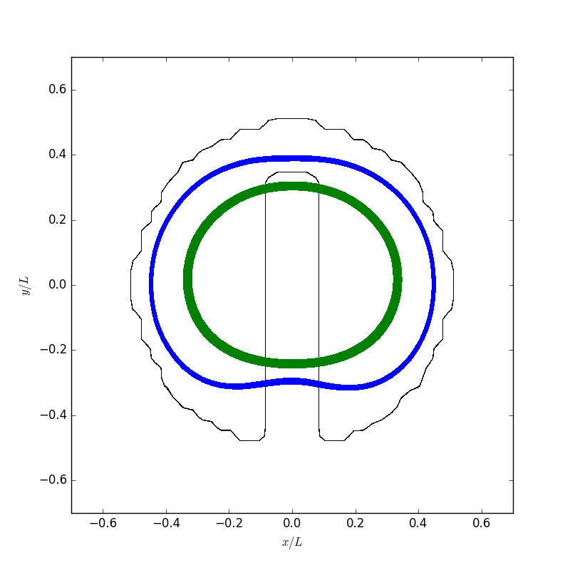
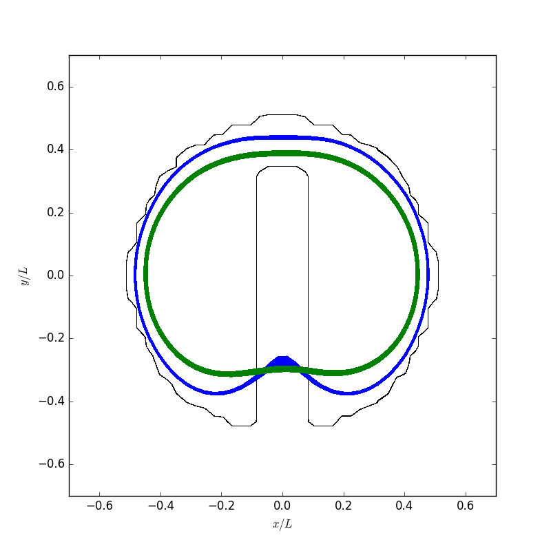
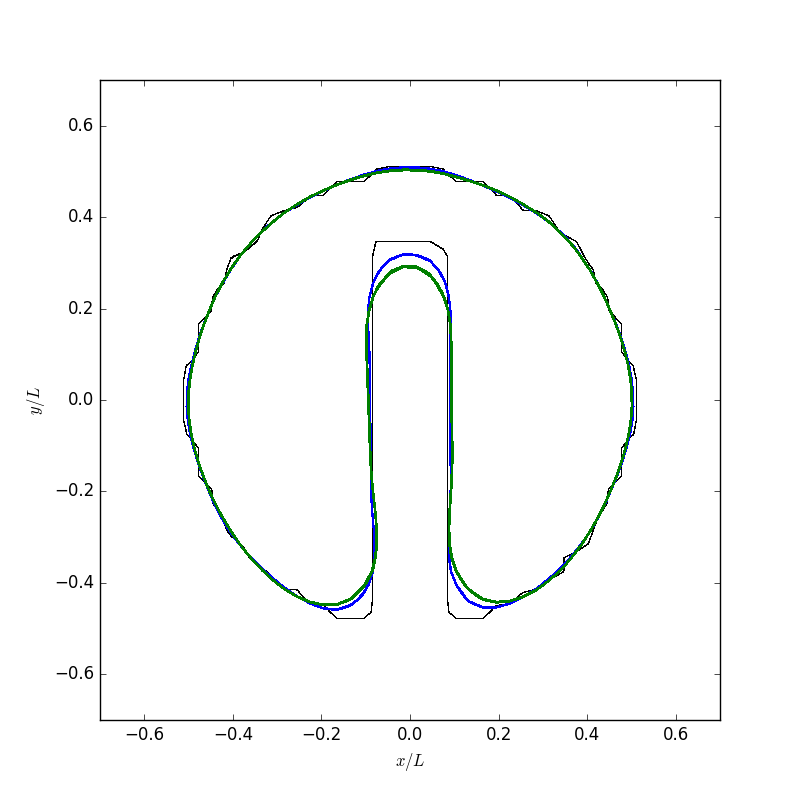
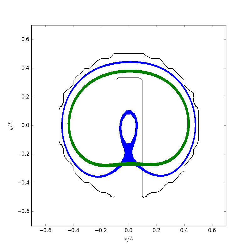
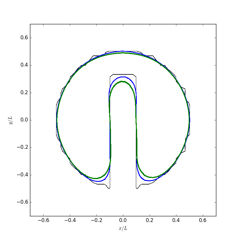
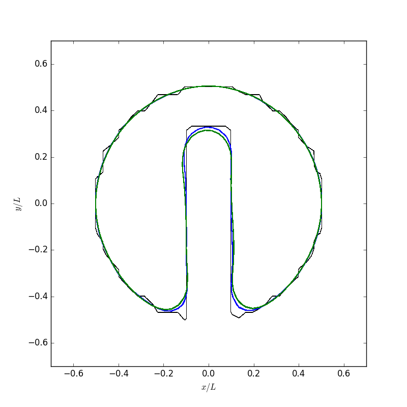
Figure 2: Results for the rotation of Zalesak’s disk. Isocontours for $\alpha\in(0.49,0.51)$. Initial field in black, after one rotation in blue, after two in green. Top row: “coarse” simulations, same number of particles as mesh nodes ( $h=H$ ). Bottom row: “fine” simulations, six particles per mesh nodes. Left column: linear FEs for mesh and particles. Middle: QCSF for the mesh, linear for the particles. Right: QCSF for both mesh and particles.

On the other hand, usage of the extended functional set results in Gibbs phenomena for this discontinuous field. Fig. 3 shows detailed contours for projFEMq and projFEM6 after two rotations. The isocontour for $\alpha=0.5$ is shown again, but the $\alpha=0$ contour reveals a corona of negative values that is more spread out in projFEM6. Values of $\alpha$ as high as $1.1$ are seen in the inner regions for projFEMq. These high values are not obtained for projFEM6, but in this case the high values are greatly eroded, with just two small slits for $\alpha=1$. This limitation is not surprising, since the extended functions have negative regions, as is apparent in condition (25) of Appendix B.

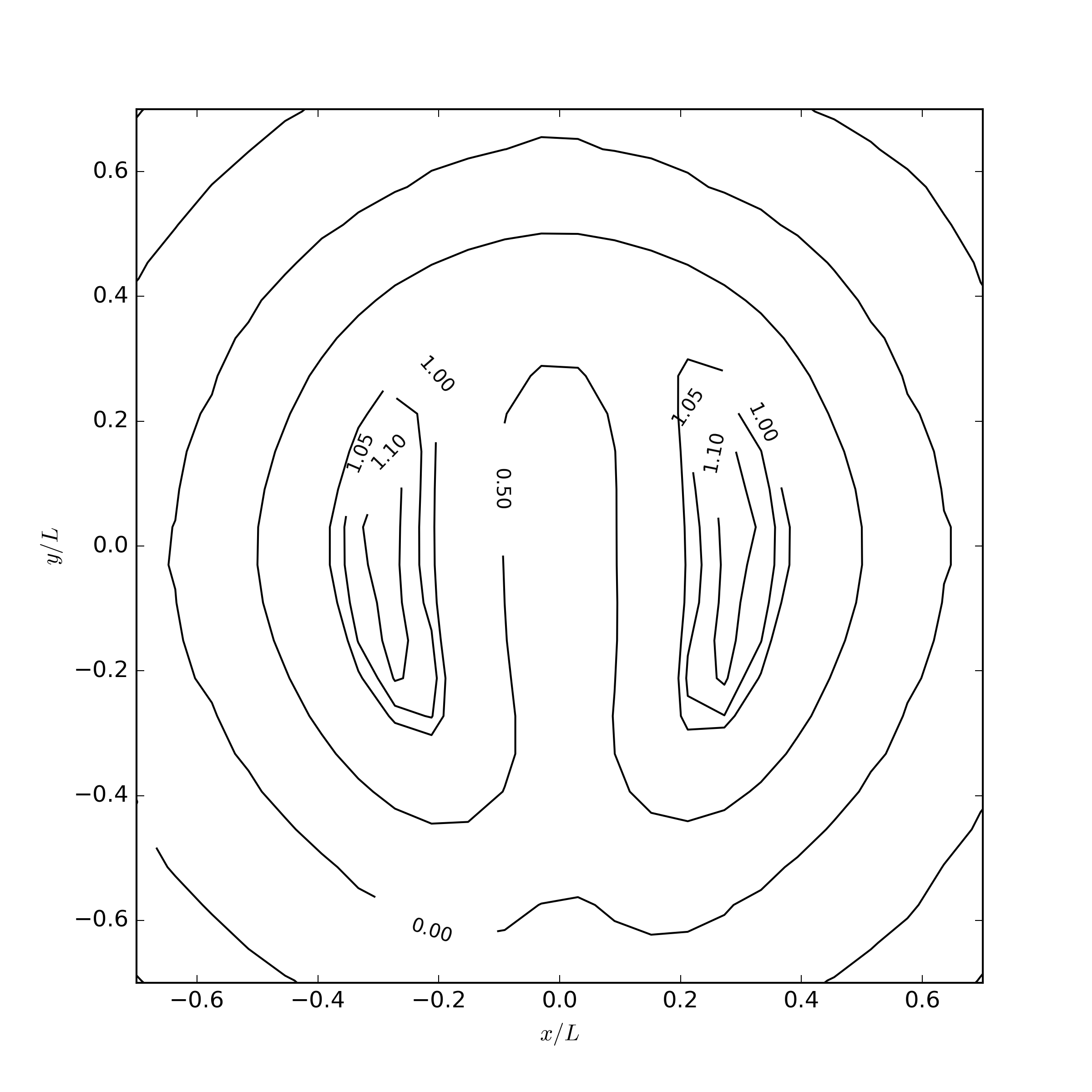
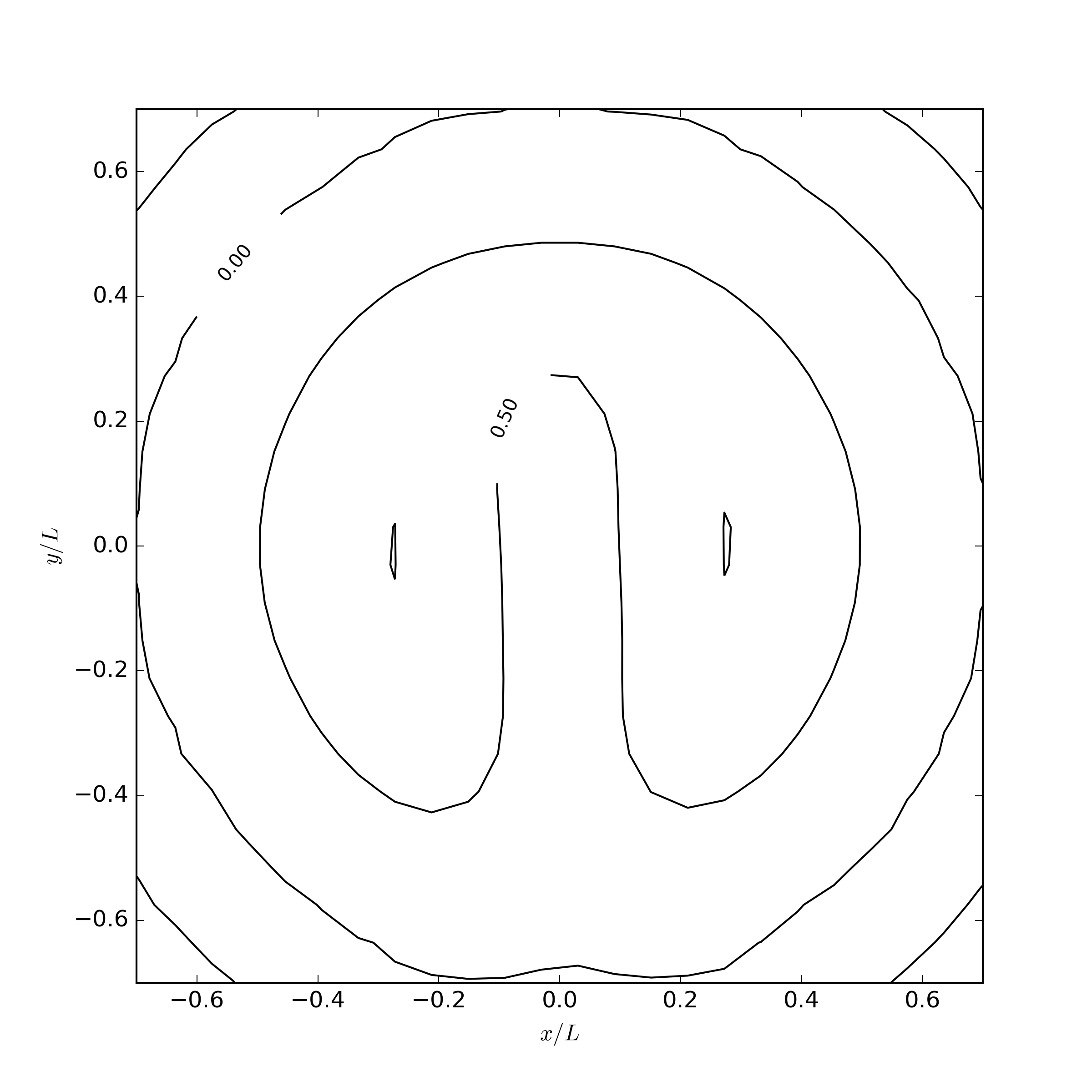
Figure 3: Results for the rotation of Zalesak’s disk. Isocontours for $\alpha\in(0,0.5,1,1.05,1.1)$ after two rotations. Left: projFEMq. Right: projFEM6.

3.2 Taylor-Green vortex sheet

This is an analytic solution to the Navier-Stokes equations for an incompressible Newtonian fluid:

$$\frac{d\mathbf{u}}{dt}=-\nabla p+\nu\nabla^{2}\mathbf{u}.$$ (14)

The solution in periodic boundary conditions is described by the velocity field

$$\mathbf{u}_{x} =f(t)\sin(kx)\cos(ky)$$ (15)

$$\mathbf{u}_{y} =-f(t)\cos(kx)\sin(ky),$$ (16)

with $k=2\pi/L$, and the pressure field

$$\frac{p}{\rho}=\frac{1}{4}f(t)^{2}\left[\cos(2kx)+\cos(2ky)\right],$$ (18)

where

$$f(t)=u_{0}\exp\left(-8\pi^{2}t^{*}/\mathrm{Re}\right).$$

The Reynolds number is defined as Re$:=u_{0}L/\nu$, and dimensionless time is $t^{*}:=tu_{0}/L$. We set $u_{0}=1$, $L=2$, and $\nu=0.01$, setting a Reynolds number Re=$200$.

For the numerical solution of the Navier-Stokes equation, a standard splitting approach is used [14]. For the partFEM case, the algorithm employed is:

1. Initialize the velocity field $\mathbf{u}^{\mathrm{m}}_{t=0}$ on the mesh, from Eq. (15).

2. Define a midpoint velocity $\mathbf{u}_{n+1/2}\approx\mathbf{u}_{n}$.

3. Move the particles a half step according to the midpoint velocity field: $\mathbf{r}_{n+1/2}=\mathbf{r}_{n}+\frac{\Delta t}{2}\mathbf{u}_{n+1/2}.$

4. Build a Delaunay triangulation from the position of the particles. Determine the coefficients needed for the evaluation of linear FEM shape functions and their integrals. Determine the matrices needed for the FEM calculation.

5. Calculate an intermediate velocity field from the equation $\mathbf{u}^{*}=\mathbf{u}_{n}+\frac{\Delta t}{2}\mu\nabla^{2}\mathbf{u}^{*}.$

6. Solve the Poisson pressure equation $\nabla^{2}p_{n+1/2}=\frac{2}{\Delta t}\nabla\cdot\mathbf{u}^{*}.$

7. Calculate new midpoint velocities $\mathbf{u}_{n+1/2}=\mathbf{u}^{*}-\frac{\Delta t}{2}\nabla p_{n+1/2}$.

8. Go to 3 until convergence in positions (i.e. the new positions are within a distance threshold from the previous iteration).

9. Move the particles a whole step: $\mathbf{r}_{n+1}=\mathbf{r}_{n}+\mathbf{u}_{n+1/2}\Delta t$.

10. Go to 2 until the end

Each of these operations is of course carried out on each of the particles, therefore we should have written $\mathbf{u}_{i,n+1/2}=\mathbf{u}_{i,n}$, etc, but the $i$ index is dropped for the sake of simplicity.

For projFEM, the procedure is very similar, with the space derivatives being calculated on the mesh (namely: solving for $\mathbf{u}^{*}$, solving for the pressure, and evaluating its gradient). The procedure is as follows, where a “$\mathrm{m}$” superscript is used to distinguish the mesh velocity field, and “$\mathrm{p}$” for the one on the particles.

1. Build the Delaunay triangulation for the mesh. Determine the coefficients needed for the evaluation of QCSF shape functions and their integrals. Determine the matrices needed for the Galerkin calculation.

2. Initialize the velocity field $\mathbf{u}^{\mathrm{m}}_{t=0}$ on the mesh, from Eq. (15).

3. At time-step $n$, define a midpoint mesh velocity $\mathbf{u}^{\mathrm{m}}_{n+1/2}\approx\mathbf{u}^{\mathrm{m}}_{n}$.

4. Project the midpoint velocity onto the particles $\mathbf{u}^{\mathrm{m}}_{n+1/2}\rightarrow\mathbf{u}^{\mathrm{p}}_{n+1/2}$.

5. Move the particles a half step according to the midpoint velocity field: $\mathbf{r}_{n+1/2}=\mathbf{r}_{n}+\frac{\Delta t}{2}\mathbf{u}^{\mathrm{p}}_{n+1/2}.$

6. Build the Delaunay triangulation for the particles. Determine the coefficients needed for the evaluation of either linear FEM shape functions (projFEM6) or QCSF (projFEMq).

7. Project the previous velocity onto the mesh, $\mathbf{u}^{\mathrm{p}}_{n}\rightarrow\mathbf{u}^{\mathrm{m}}_{n}$.

8. Calculate an intermediate mesh velocity field from the equation $\mathbf{u}^{*}=\mathbf{u}^{\mathrm{m}}_{n}+\frac{\Delta t}{2}\mu\nabla^{2}\mathbf{u}^{*}.$

9. Solve the Poisson pressure equation on the mesh $\nabla^{2}p_{n+1/2}=\frac{2}{\Delta t}\nabla\cdot\mathbf{u}^{*}.$

10. Calculate new midpoint mesh velocities $\mathbf{u}^{\mathrm{m}}_{n+1/2}=\mathbf{u}^{*}-\frac{\Delta t}{2}\nabla p_{n+1/2}$.

11. Go to 4 until convergence in positions (i.e. the new positions of the particles are within a distance threshold from the previous iteration).

12. Move the particles a whole step: $\mathbf{r}_{n+1}=\mathbf{r}_{n}+\mathbf{u}^{\mathrm{p}}_{n+1/2}\Delta t$. Calculate new velocities: $\mathbf{u}^{\mathrm{p}}_{n+1}=2\mathbf{u}^{\mathrm{p}}_{n+1/2}-\mathbf{u}^{\mathrm{p}}_{n}$

13. Build the Delaunay triangulation for the particles. Determine the coefficients needed for the evaluation of either linear FEM shape functions (projFEM6) or QCSF (projFEMq).

14. Project the new velocities onto the mesh, $\mathbf{u}^{\mathrm{p}}_{n+1}\rightarrow\mathbf{u}^{\mathrm{m}}_{n+1}$.

15. Go to 2 until the desired number of steps.

An obvious computational advantage compared to the previous, all-particle, partFEM is that the mesh shape functions and the matrices needed for the spatial differential equations are calculated, and treated, only once in the course of the simulation, at step 1. However, the particle shape functions are calculated at every step since they are still needed for the projection procedure.

The projFEM6 method is very similar to the pFEM2 methods of Ref. [8], with fully explicit integration of the positions and fully implicit integration on the mesh (a value of $\theta=1$ in pFEM2’s notation). The main difference is that our integrators are simple half-step integrators, while in pFEM2 the values of the fields are integrated following the streamlines. The projFEMq method further deviates from pFEM2 by including QCSF (see Table 1).

In Fig. 4 we show a snapshot of a simulation that has started from a regular arrangement, for a number of particles $N=20\times 20$, a time-step of $\Delta t^{*}=0.025$ (corresponding to a Courant number of Co${}_{H}=0.5$), at a reduced time $T^{*}=1$. The top left figure shows the particles’ position and pressure field for the partFEM simulation. At its right, the pressure field for the mesh in a projFEMq simulation is plotted. The corresponding particles are plotted at the bottom left, with the same color code (actually, the pressure field is calculated only on the mesh, but here it has been interpolated on the particles for visualization purposes). Finally, the figure on its right shows the particles for an projFEM6 simulation (the mesh result is visually very similar to the one above and is therefore not shown).

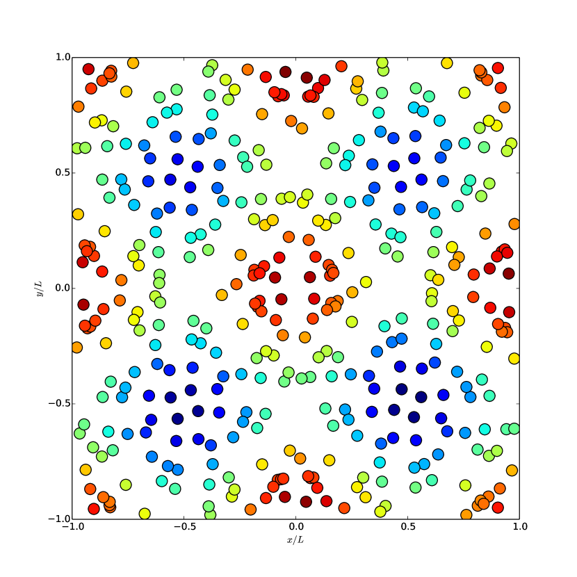
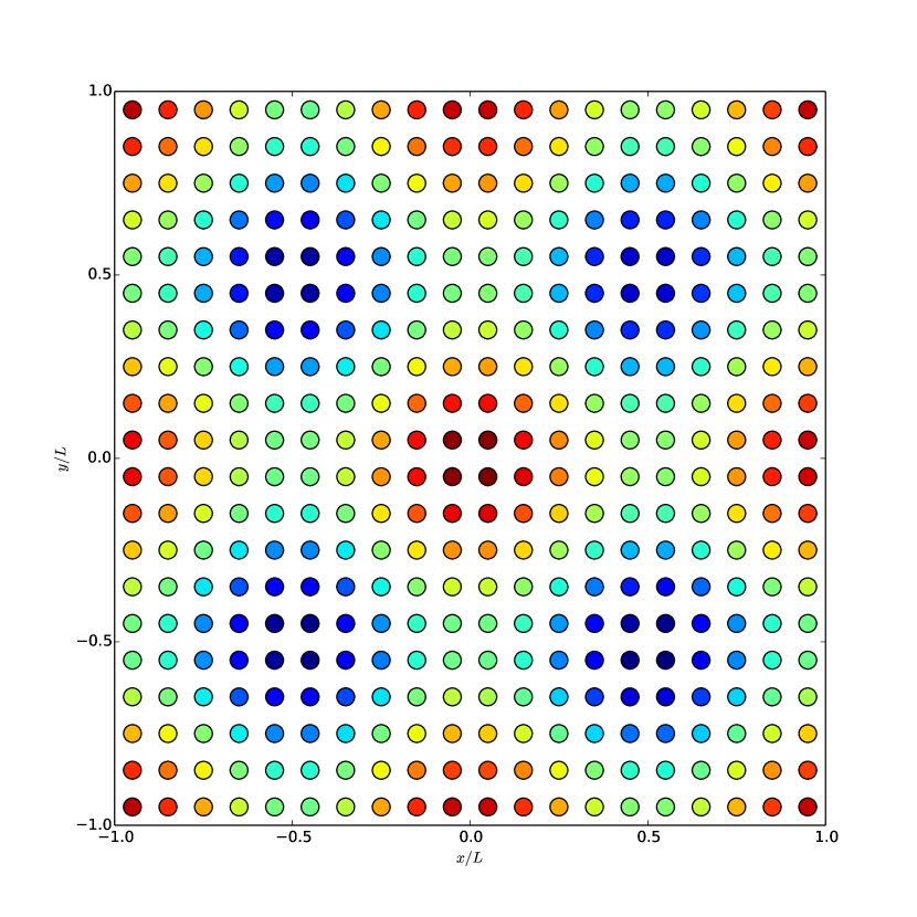
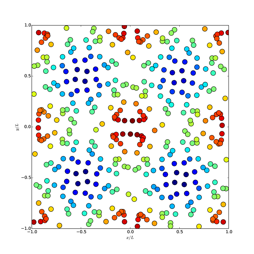
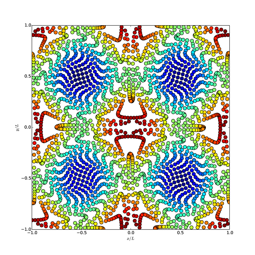
Figure 4: Results for the pressure field at $T^{*}=1$. From top left: partFEM, projFEMq (field on the mesh), projFEMq (field on the particles), projFEM6 (field on the particles).

In order to quantify the accuracy of the different methods, the relative $L_{2}$ distance between a given field $\phi$ obtained by simulation and its exact value is computed:

$$L_{2}:=\sqrt{\frac{\sum_{i=1}^{N}V_{i}\left|\phi(\mathbf{r}_{i})-\phi_{i}\right|^{2}}{\sum_{i=1}^{N}V_{i}|\phi(\mathbf{r}_{i})|^{2}}},$$ (19)

where $\phi(x_{i})$ is the exact solution at particle $i$ and $\phi_{i}$ the computed one on that particle position. The volume of particle $i$ is defined as $V_{i}:=\int\psi_{i}(\mathbf{r})d\mathbf{r}$. The expression results from the discretization of the $L_{2}$ distance between two functions, $L_{2}:=\int(f(\mathbf{r})-g(\mathbf{r}))^{2}d\mathbf{r}$. The same measure may be evaluated for mesh nodes, with very similar results. For vector fields this distance is defined with $|\cdots|^{2}$ meaning the squared vector modulus.

This error is expected to start at a very low value and increase approximately linearly as the simulation proceeds. In order to compare between methods, in Fig. 5 the value of this error at $T^{*}=1$ is plotted, for the velocity and pressure fields. At this time, $f(T)=\exp(-8\pi^{2}/200)=0.67$, so that the velocity field should have decreased to about $67\%$ of its initial value, and the pressure, $45\%$.

The error for the velocity field (left subfigure) is seen to decrease with $\Delta t$. The value of $h$ (and, for projFEM methods, $H$) also decreases as $\Delta t$, in order to fix a Courant number of Co${}_{H}=0.5$. As expected, the order of convergence of the error agree with a $\Delta t^{2}$ power low both for partFEM and projFEMq. The error of projFEM6 is seen to vanish only as $\Delta t^{1}$. The error for the pressure (right subfigure) vanishes roughly similarly: as $\Delta t^{2}$ for partFEM and projFEMq, and as $\Delta t^{1}$ for projFEM6. (This error is evaluated at the nodes, since the pressure field is obtained on them and need not be projected onto the particles.)

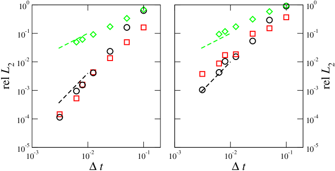
Figure 5: $L_{2}$ error of the velocity (left) and pressure (right) fields at time $T^{*}=1$ versus time step $\Delta t$. Black circles: projFEMq method, red squares: partFEM, green diamonds: projFEM6. Dashed lines are power-laws plotted for convenience. Left: $\Delta t^{2}$ (lower black line), $\Delta t$ (upper green line). Right: $\Delta t^{2}$ (lower black line), $\Delta t$ (upper green line).

A relevant question when comparing different methods is their efficiency in terms of CPU time. By plotting the error as a function of CPU time one may discriminate between a straightforward method that performs quickly, and a more sophisticated one that needs more computational resources. Results for the latter clearly depend on the machine, but if we employed a faster one, it is likely that the CPU times of each simulation run will be sped up by roughly the same factor. This would simply result in a horizontal translation of all the curves in a logarithmic scale. Results do depend on the particular linear algebra algorithm used, details can be found in Appendix A.

In Fig. 6 the relative $L_{2}$ error at simulation time $T^{*}=1$ is plotted as a function of the CPU time $T_{\mathrm{CPU}}$. Regarding the velocity field (left subfigure in Fig. 5), the convergence for partFEM is as $T_{\mathrm{CPU}}^{-0.7}$, but is slightly superior, as $T_{\mathrm{CPU}}^{-0.85}$, for projFEMq, due to the latter using direct methods for numerical algebra. Nevertheless, partFEM may be preferable at lower resolutions, as the crossover takes place at the finest, longest, simulations. The convergence of projFEM6 is a rather poor $T_{\mathrm{CPU}}^{-0.3}$. For the pressure (right subfigure), the convergence for partFEM is about $T_{\mathrm{CPU}}^{-0.4}$, for projFEMq it is $T_{\mathrm{CPU}}^{-0.7}$, and for projFEM6 it is $T_{\mathrm{CPU}}^{-0.3}$. For this quantity the convergence of projFEMq is clearly superior, and the crossover with partFEM occurs at intermediate resolutions, due to the quite different rates of convergence.

Therefore, one may conclude from these observations that the higher computational cost of a projFEM method can be compensated at high resolutions by its higher accuracy. When running the simulations it is apparent how the partFEM method proceeds at a steady pace, while the projFEM methods employs some time in the initial set-up of the matrices, and then starts, taking more time at each time step, but producing more accurate results.

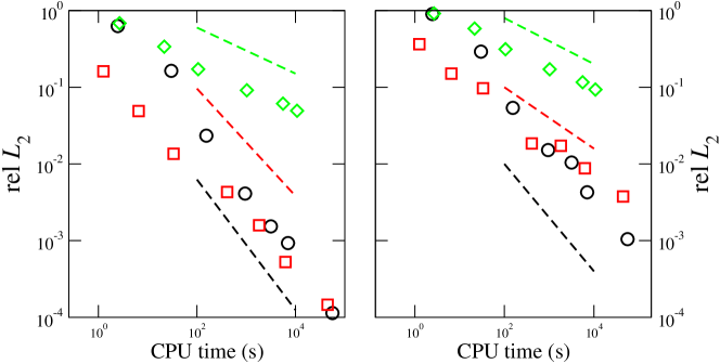
Figure 6: $L_{2}$ error of the velocity (left) and pressure (right) fields at time $T^{*}=1$ versus CPU time. Black circles: projFEMq method, red squares: partFEM, green diamonds: projFEM6. Dashed lines are power-laws plotted for convenience. Left: $T_{\mathrm{CPU}}^{-0.85}$ (lower black line), $T_{\mathrm{CPU}}^{-0.7}$ (middle red line), $T_{\mathrm{CPU}}^{-0.3}$ (upper green line). Right: $T_{\mathrm{CPU}}^{-0.7}$ (lower black line), $T_{\mathrm{CPU}}^{-0.4}$ (middle red line), $T_{\mathrm{CPU}}^{-0.3}$ (upper green line).

3.3 Rayleigh-Taylor instability

In this section, we qualitatively compare the behavior of the methods discussed, for the numerical solution of the Rayleigh-Taylor instability, including results from OpenFOAM. This well-known benchmark case consists of two phases in a gravitational field, with the denser layer on top. The interface is perturbed initially, and plumes develop. As we do not want to consider wall boundary conditions in this work, periodic boundary conditions are employed, and a “gravity” of the form

$$\vec{f}_{\mathrm{g}}=-g(2\alpha-1)\vec{u}_{y},$$

acts on each particle, where $\alpha$ is a color function with values $1$ for the heavier phase and $0$ for the lighter phase. In this way, heavier particles are pulled downwards and lighter particles, upwards. The density is kept constant, and the value of $g$ is set to $1$ for simplicity.

The CGAL libraries used in the Delaunay construction currently implement only square periodic boundary conditions, therefore a square simulation cell $(-1,1)\times(-1,1)$ is considered, instead of the usual $1:4$ aspect ratio. The initial interface is perturbed by a cosine shape: $\eta=-0.05\cos(4\pi x)$, giving rise to four identical plumes (or similar, for a randomly perturbed initial distribution). We set $\nu=3.53\times 10^{-4}$, in order to set a Reynolds number of Re$:=\sqrt{2L\sqrt{gL}}/\nu=1000$.

In Fig. 7 results are shown for the partFEM method, the projFEMq, and the projFEM6. Results from the OpenFOAM finite volume method software are also included (see details in Appendix A.)

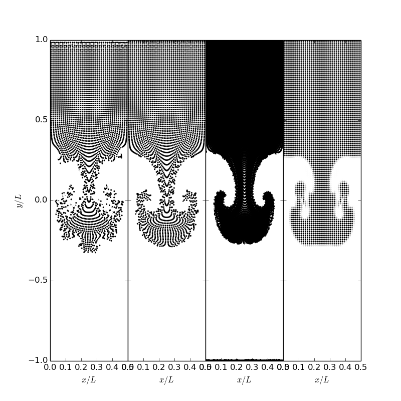
Figure 7: Rayleigh-Taylor instability. Color field at $t=1.32$, with black for particles with $\alpha=1$, and white (not visible, for clarity), for $\alpha=0$. From left to right: partFEM method, projFEMq, projFEM6, and OpenFOAM (the latter in gray levels). Only the middle section is shown, the other parts of the simulation being exactly repeated.

The partFEM simulations seem to underestimate the viscosity, since they give rise to an interface that is more distorted than the others. The projFEMq and projFEM6 yield similar results, with the latter producing smoother results at the cost of using $6$ particles per node instead of just one. These results may be compared against the OpenFOAM result, which uses the same parameters and mesh resolution. Note that OpenFOAM uses a volume-of-fluid algorithm which leads to species diffusion, manifest in the appearance of gray nodes that have intermediate values of the color field. However, the $\alpha$ field, when associated to the particles, should have in this problem crisp values of either $0$ or $1$. In addition, OpenFOAM results are clearly affected by the underlying Eulerian mesh, as it is apparent from the much less curved plume interface. It therefore seems that OpenFOAM results are affected by numerical artifacts in this case. These artifacts are absent in the projection methods considered in this work.

4 Discussion

There are two different points of view regarding the interpretation of projPFEM methods. In one of them, the simulation is Lagrangian in spirit: the fluid particles move while carrying the fields, and the mesh is merely used as a tool to evaluate space derivatives. The other approach is Eulerian in spirit: the mesh contains the fields and the particles are only used to advect them from one time step to the next one. The resulting numerical algorithms are very similar if the particles are kept from one time-step to the next, but the latter point of view allows for greater flexibility in the treatment of the particles: they may be re-created at (or, around) mesh nodes each time steps, moved, and destroyed. We have explored this possibility, and the main difference is a better convergence (both as a function of $\Delta t$ and of CPU time) of the velocity field at high resolutions, while that of the pressure field is relatively unaffected. Results are not shown for the sake of brevity. It is worth mentioning that several other variants (such as “projFEMq6”, with six times more particles than mesh nodes, but quadratic functions for both, bottom right results of Fig. 2) have also been considered, with results that seem better as far as convergence with $\Delta t$ is concerned, but turn out to be quite similar when CPU time is considered.

5 Conclusions

We have presented a combination of pFEM-like Lagrangian particles with a standard FEM Eulerian mesh. Our results confirm the findings of Ref. [8], in which the projection errors, especially from particles to mesh, are identified as the culprits of slow convergence of the method. We restore an acceptable convergence rate by including quadratically consistent shape functions for the interpolation given simply in terms of products of standard linear finite element basis functions. The method is first validated on the Zalesak’s disk problem, which is used to screen possible variations on the method. These are later used on the Taylor-Green vortex sheet flow, our main benchmark. Convergence is not only tested as a function of mesh refinement, but also in terms of CPU time, which is, in our opinion, a critical and useful test to compare widely different methods.

Our results show that the quadratic consistent method for projection from mesh to particles and back gives a convergence superior to previous projection methods in terms of the order of convergence and in terms of CPU time. The method offers a very promising route to deal with problems where a Lagrangian description is helpful (as in fluid-structure interaction with large deformations, free surfaces, sloshing, splashing, etc. [11, 8]), and high resolution results are required.

Of course, the procedure should be extended in many ways. Boundary conditions, other than just periodic ones, should be considered. The method should also be extended to 3D problems. Such an extension, even if straightforward conceptually, could bring about technical difficulties, specially in complicated geometries. In both 2D and 3D application the method clearly relies on a rather uniform particle distribution, a condition that may fail in some cases. A possible remedy would be re-creating the particles periodically, as pointed out in the previous section.

We finally stress once again that only a simple interpolation procedure is used for projection. Other possibilities, such as Galerkin projection, may provide superior results and are worth considering in the future. The authors are also currently evaluating the performance of procedures in which projection involves convolutions with projection kernel functions.

Appendix A Numerical methods

For all computational geometry procedures the CGAL 4.7 libraries [15] are used. In particular, the 2D Periodic Delaunay Triangulation package, overloading the vertex base to contain the relevant fields, and the face base to contain information relevant to the edges.

The Eigen 3.0 linear algebra libraries [16] are also employed. For the small linear algebra problem involved in the calculation of the $A$ coefficients, SVD is used, with automatic rank detection. For the large problems involved in the Galerkin procedure, the sparse matrix package is used. The linear systems are solved iteratively for partFEM, by the BiCGSTAB method. For projFEM a direct method is employed, with best results obtained using the CHOLMOD [17] routines of the suitesparse project (through Eigen wrappers for convenience, class CholmodSupernodalLLT). Slightly worse results are obtained with eigen’s build-in SimplicialLDLT class.

The OpenFOAM 3.0.1 finite volume method software has also been used. Periodic (“cyclic”) boundary conditions are selected, on a 2D square simulation cell. The utility funkySetFields, a part of the swak4Foam extension package, is used to set the initial interface. In order to mimic our simulations, we have modified the interFoam solver so that only the pressure field is used (not the “p_rgh” one, which would include the gravity), and to add an additional term, $(2\alpha-1)\rho g$, to the right-hand side of the momentum equation.

Our computations took place on a 4-core Pentium 4 machine with 16 Gb RAM.

Appendix B Quadratic correction

For an arbitrary arrangement of $N$ nodes labeled by the index $\mu$, let us consider a set of functions $\{\phi_{\mu}\}$ that reconstruct constant functions exactly (a property known as partition of unity):

$$\sum^{N}_{\mu=1}\phi_{\mu}(\mathbf{r})=1.$$ (20)

We will suppose that linear functions are also exactly reconstructed by this set (a property known as the local co-ordinate):

$$\sum^{N}_{\mu=1}\phi_{\mu}(\mathbf{r})\mathbf{r}_{\mu}=\mathbf{r}.$$ (21)

These two properties combined define “linear precision”. These are satisfied by many functional sets, including the well-known linear finite elements (FE) shape functions, natural neighbor interpolants (either Sibsonian or otherwise) [18], and LME and SME interpolants [19, 20].

Only linear FE shape functions are considered here. In 1D, the nodal functions for node $\nu$ is continuous and piece-wise linear, with $\phi_{\mu}(x)$ going from $0$ at $x_{\mu-1}$ to $1$ at $x_{\mu}$, back to $0$ at $x_{\mu+1}$. They are zero outside the segment $(x_{\mu-1},x_{\mu+1})$. Similarly, in 2D $\phi_{\mu}(\mathbf{r})$ is a pyramid of height $1$ at node $\mu$ with straight edges that connect the apex with the neighboring nodes. These neighbors are determined by an underlying 2D triangulation; there are many possible ones, but we choose, as is customary, the unique (except for possible degeneracies) Delaunay triangulation [21], thus defining natural neighbors.

The FE shape functions do not comply with quadratic precision in general:

$$\sum^{N}_{\mu=1}\mathbf{r}_{\mu}\mathbf{r}_{\mu}^{\mathrm{t}}\phi_{\mu}(\mathbf{r})\neq\mathbf{r}\mathbf{r}^{\mathrm{t}}.$$ (22)

We here consider an “extended” set of shape functions derived from the FE $\{\phi_{\mu}\}$ shape set, with functions:

$$\psi_{\mu}(\mathbf{r}) :=\phi_{\mu}(\mathbf{r})+\sum_{\nu\sigma}A_{\mu\nu\sigma}\phi_{\nu}(\mathbf{r})\phi_{\sigma}(\mathbf{r}),$$ (23)

i.e. a linear combination of the original functions and their pair-wise products. The inclusion of these products extends the spatial support of the original functions (hence their name; the number of functions in each set is the same.)

The coefficients will be taken to be symmetric with respect to the last two indices: $A_{\mu\nu\sigma}=A_{\mu\sigma\nu}$, and are determined so as to fulfill not only Eqs. (20) and (21), but also to comply with quadratic precision:

$$\sum^{N}_{\mu=1}\mathbf{r}_{\mu}\mathbf{r}_{\mu}^{\mathrm{t}}\psi_{\mu}(\mathbf{r})=\mathbf{r}\mathbf{r}^{\mathrm{t}}.$$ (24)

One way to achieve this is by requiring that the coefficients $A_{\mu\nu\sigma}$ satisfy

$$\sum^{N}_{\mu=1}A_{\mu\nu\sigma} =0$$ (25)

$$\sum^{N}_{\mu=1}\mathbf{r}_{\mu}A_{\mu\nu\sigma} =0$$ (26)

$$\sum^{N}_{\mu=1}\mathbf{r}_{\mu}\mathbf{r}_{\mu}^{\mathrm{t}}A_{\mu\nu\sigma} =\frac{1}{2}\left(\mathbf{r}_{\nu}\mathbf{r}_{\sigma}^{\mathrm{t}}+\mathbf{r}_{\sigma}\mathbf{r}_{\nu}^{\mathrm{t}}-\mathbf{r}_{\nu}\mathbf{r}_{\nu}^{\mathrm{t}}-\mathbf{r}_{\sigma}\mathbf{r}_{\sigma}^{\mathrm{t}}\right)$$ (27)

as can be checked explicitly. The last identity can be rewritten with the help of the first two as

$$\sum^{N}_{\mu=1}(\mathbf{r}_{\mu}-\mathbf{r}_{\nu})(\mathbf{r}_{\mu}-\mathbf{r}_{\sigma})^{\mathrm{t}}A_{\mu\nu\sigma} =-\frac{1}{2}(\mathbf{r}_{\nu}-\mathbf{r}_{\sigma})(\mathbf{r}_{\nu}-\mathbf{r}_{\sigma})^{\mathrm{t}},$$ (28)

which is clearly translation and rotation invariant.

We want to have the largest number of coefficients $A_{\mu\nu\sigma}$ equal to zero and, if possible, only different from zero if $\mu,\nu,\sigma$ are some kind of neighbors. For every pair $\nu,\sigma$ a set of equations must be fulfilled. It seems reasonable to look only for pairs that are neighboring. Then, we require that $A_{\mu\nu\sigma}=0$ if $\nu,\sigma$ are not neighbors or if $\nu=\sigma$. Then, we also require that $A_{\mu\nu\sigma}=0$ if $\mu$ is not a neighbor (in some sense) of either $\nu$ or $\sigma$.

Notice that while this is, in principle, a purely geometrical calculation that is not directly related to the original set of functions, the particular definition of the geometrical concept of “neighbor” should be tied to the particular set employed. In the case of standard FE examined in this work, this means Delaunay neighbors (i.e. connected by an edge of the triangulation). For a full description of the procedure, we refer the reader to [13].

References

- [1] Versteeg HK, Malalasekera W. An introduction to computational fluid dynamics: the finite volume method. Pearson Education, 2007.
- [2] Evans M, Harlow F. The particle-in-cell method for hydrodynamic calculations. Technical Report LA-2139, Los Alamos Scientific Laboratory 1957.
- [3] Amsden A. The particle-in-cell method for the calculation of the dynamics of compressible fluids. Technical Report LA-3466, Los Alamos Scientific Laboratory 1966.
- [4] Chaniotis AK, Poulikakos D, Koumoutsakos P. Remeshed smoothed particle hydrodynamics for the simulation of viscous and heat conducting flows. Journal of Computational Physics 2002; 182(1):67–90.
- [5] Feldman J, Bonet J. Dynamic refinement and boundary contact forces in SPH with applications in fluid flow problems. International Journal for Numerical Methods in Engineering 2007; 72(3):295–324.
- [6] Marrone S, Di Mascio A, Le Touzé D. Coupling of smoothed particle hydrodynamics with finite volume method for free-surface flows. Journal of Computational Physics 2015; .
- [7] Quinlan NJ, Lobovskỳ L, Nestor RM. Development of the meshless finite volume particle method with exact and efficient calculation of interparticle area. Computer Physics Communications 2014; 185(6):1554–1563.
- [8] Idelsohn S, Oñate E, Nigro N, Becker P, Gimenez J. Lagrangian versus Eulerian integration errors. Computer Methods in Applied Mechanics and Engineering 2015; 293:191–206.
- [9] Stanton M, Sheng Y, Wicke M, Perazzi F, Yuen A, Narasimhan S, Treuille A. Non-polynomial Galerkin projection on deforming meshes. ACM Transactions on Graphics (TOG) 2013; 32(4):86.
- [10] Rapún ML, Terragni F, Vega JM. LUPOD: Collocation in POD via LU decomposition. Journal of Computational Physics 2017; 335:1 – 20.
- [11] Oñate E, Idelsohn SR, del Pin F, Aubry R. The particle finite element method - an overview. International Journal of Computational Methods 2004; 1(2):267–307.
- [12] Liu M, Liu G, Lam K. Constructing smoothing functions in smoothed particle hydrodynamics with applications. Journal of Computational and Applied Mathematics 2003; 155(2):263 – 284.
- [13] Duque D, Español P. Extending linear finite elements to quadratic precision in arbitrary meshes. Applied Mathematics and Computation 2016; Accepted for publication.
- [14] Codina R. Pressure stability in fractional step finite element methods for incompressible flows. Journal of Computational Physics 2001; 170(1):112–140.
- [15] CGAL Editorial Board. Cgal, Computational Geometry Algorithms Library. Http://www.cgal.org.
- [16] Guennebaud G, Jacob B, et al.. Eigen v3. http://eigen.tuxfamily.org 2010.
- [17] Chen Y, Davis TA, Hager WW, Rajamanickam S. Algorithm 887: Cholmod, supernodal sparse cholesky factorization and update/downdate. ACM Trans Math Software 2009; 35(3).
- [18] Belikov V, Ivanov V, Kontorovich V, Korytnik S, Semenov AY. The non-Sibsonian interpolation: A new method of interpolation of the values of a function on an arbitrary set of points. Computational mathematics and mathematical physics 1997; 37(1):9–15.
- [19] Arroyo M, Ortiz M. Local maximum-entropy approximation schemes: a seamless bridge between finite elements and meshfree methods. International Journal for Numerical Methods in Engineering 2006; 65(13):2167–2202, doi:10.1002/nme.1534. URL http://dx.doi.org/10.1002/nme.1534.
- [20] Cyron CJ, Arroyo M, Ortiz M. Smooth, second order, non-negative meshfree approximants selected by maximum entropy. International Journal for Numerical Methods in Engineering 2009; 79(13):1605–1632.
- [21] Okabe A, Boots B, Sugihara K, Chiu SN. Spatial tessellations: Concepts and applications of Voronoi diagrams. 2nd edn., Probability and Statistics, Wiley: NYC, 2000. 671 pages.