Characterizing error propagation in quantum circuits: the Isotropic Index.

Abstract

This paper presents a novel index in order to characterize error propagation in quantum circuits by separating the resultant mixed error state in two components: an isotropic component, that quantifies the lack of information, and a dis-alignment component, that represents the shift between the current state and the original pure quantum state. The Isotropic Triangle, a graphical representation that fits naturally with the proposed index, is also introduced. Finally, some examples with the analysis of well-known quantum algorithms degradation are given.

I Introduction

The design and construction of reliable quantum computers is one of the greatest challenges of these decades. Long-lived quantum state superposition, entanglement maintenance and manipulation of large-qubits systems require the analysis of several technological implementation aspects of quantum systems Ladd_2010 .

One of the most important problems is that quantum systems cannot be completely isolated from the environment. This fact, together with imperfections in gate applications, state preparations and others, induces errors in any quantum computation Knill_1998 Gottesman_2010 Devitt_2013 . While there is a fault-tolerant model of quantum computing based on the correction of errors below a certain threshold Gottesman_1998 Aharonov_2008 this method is very expensive in computational resources. Therefore, the development of new tools in order to analyze the effect and propagation of quantum errors is an important issue.

This paper presents a novel index, the Isotropic Index, useful to identify uncorrectable components of mixed quantum states, the isotropic component; and the dis-alignment with respect to an original reference pure state.

The structure of the paper is as follows. Isotropic errors model and the concept of isotropic error state are introduced in section II. In section III we define the Isotropic Index and its graphical representation: the Isotropic Triangle. This representation gives a new perspective in the analysis of the performance loss in quantum algorithms. The relation between the isotropic states defined in Horodecki_1999 and isotropic error states is presented in section IV.

In later sections, V and VI, the index is used to explain the degradation of results in two well-known quantum algorithms: Grover’s quantum search Grover_1997 and Shor’s quantum error-correcting code Shor_1995 . In both cases depolarizing channel models are used.

II Isotropic errors

In order to define an isotropic error state, a quantum state obtained from a time-independent isotropic error process, it is useful to introduce the definition of such error model as in GarciaLopez_2003A and GarciaLopez_2007A .

Definition 1 (Time-independent isotropic error model).

A time-independent isotropic error process, with an $n$-qubits pure quantum state $|\psi\rangle$ as the reference state, is a stochastic process $f(|\psi\rangle,0,t)$, $t\geq 0$, that holds:

• At $t=0$, the density probability distribution is $f(|\psi\rangle,0,0)=\delta(|\psi\rangle)$, i.e. there is no error and the state is $|\psi\rangle$ with probability equal to $1$.

• The density probability distribution $f(|\psi\rangle,0,t_{k})$ is isotropic for all $t_{k}$. Let $|\psi(t_{k})\rangle$ be the random variable at $t_{k}$. The probability of obtaining the state $|\phi\rangle$ depends only on the quantum distance between $|\psi\rangle$ and $|\phi\rangle$,

  $$P\left(|\psi(t_{k})\rangle=|\phi\rangle\right)=F(\mathcal{D}\left(|\psi\rangle,|\phi\rangle\right)).$$ (1)

• For all $t_{k}$ and $t_{k+1}$, $t_{k}<t_{k+1}$, $f(|\psi\rangle,0,t_{k})$ and $f(|\psi\rangle,t_{k},t_{k+1})$ are independent.

With the purpose of obtaining a closed form for an isotropic error state, we consider the reference state (r.s.) as the basis state $|0\rangle$ (for a general formulation with r.s. $|\psi\rangle$, one only needs a basis change).

According to the definition a ensemble of states

$$|\psi(t_{k})\rangle=a_{0}(k)|0\rangle+a_{1}(k)e^{i\varphi_{1}(k)}|1\rangle+\dots+a_{2^{n}-1}(k)e^{i\varphi_{2^{n}-1}(k)}|2^{n}-1\rangle,$$ (2)

is an (mixed) isotropic error state (r.s. $|0\rangle$) if holds

• $|i\rangle$, $0\leq i\leq 2^{n}-1$, the canonical basis vectors (decimal notation),

• $\varphi_{i}(k)$ random variables with uniform distribution in $[0,2\pi)$ (the distance does not depend on the relative phases) and

• $a_{i}(k)$, random variables in $[0,1]$ subject to the constraints

  • $\forall k$, $\sum_{i=0}^{2^{n}-1}a_{i}^{2}(k)=1$,

  • $a_{i}(k)$, $1\leq i\leq 2^{n}-1$, have the same probability distribution.

Remark.

In this case both the distance $\mathcal{D}\left(|0\rangle,|\psi(t_{k})\rangle\right)$ and the probability distribution depend only on $a_{0}(k)$.

II.1 Density operators

The density matrix corresponding to the quantum state in (2) is

$$\rho=E\left[\,|\psi(t_{k})\rangle\langle\psi(t_{k})|\,\right]=E\left[\left(\gamma_{ij}(k)\right)\right],$$ (3)

where $E[\cdot]$ is the expected value of the random matrix and, for $1\leq i,j\leq 2^{n}-1$,

• $\gamma_{ll}(k)=a_{l}^{2}(k)$, $\forall i=j=l$,

• $\gamma_{0m}(k)=a_{0}(k)a_{m}(k)e^{-i\varphi_{m}(k)}$, $\forall j=m\neq 0$,

• $\gamma_{l0}(k)=a_{l}(k)a_{0}(k)e^{i\varphi_{l}(k)}$, $\forall i=l\neq 0$,

• y $\gamma_{lm}(k)=a_{l}(k)a_{m}(k)e^{i\left({\varphi_{l}(k)-\varphi_{m}(k)}\right)}$, $\forall l\neq m$.

As a direct consequence of the hypothesis made in (2), one has

• $E\left(e^{i\varphi_{i}(k)}\right)=0$,

• $E\left(a_{i}(k)a_{j}(k)e^{i\left(\varphi_{i}(k)-\varphi_{j}(k)\right)}\right)=E\left(a_{i}(k)a_{j}(k)\right)E\left(e^{i\varphi_{i}(k)}\right)E\left(e^{-i\varphi_{j}(k)}\right)=0$

• $E\left(a_{0}(k)\right)=\lambda_{0}$,

• $E\left(a_{i}(k)\right)=\lambda_{1},\forall\,i,\,1\leq i\leq 2^{n}-1$,

• $(2^{n}-1)\lambda_{1}+\lambda_{0}=1$.

Therefore, the mixed density matrix $\rho_{iso}$ representing an isotropic error state (with r.s. $|0\rangle$) has the form

$$\rho_{iso}=\left[\begin{array}[]{cccc}\lambda_{0}&0&0&0\\ 0&\lambda_{1}&0&0\\ \vdots&\vdots&\ddots&\vdots\\ 0&0&\cdots&\lambda_{1}\end{array}\right].$$ (4)

Definition 2 (Isotropic error state).

Let $|\psi\rangle$ be a reference state and $M$ a basis change matrix so that $|0\rangle=M|\psi\rangle$. A mixed state $\rho$ is an isotropic error state (r.s.$|\psi\rangle$) if the the state $\bar{\rho}=M\rho M^{\dagger}$ has the form (4) and can be expressed as

$$\bar{\rho}=\left\{\begin{array}[]{lcr}\left(2^{n}\lambda_{1}\right)\frac{I}{2^{n}}+\left(\lambda_{0}-\lambda_{1}\right)\rho_{0},&&\lambda_{0}\geq\lambda_{1}\\ \\ \left(2^{n}\lambda_{0}\right)\frac{I}{2^{n}}+\left(2^{n}-1\right)\left(\lambda_{1}-\lambda_{0}\right)\rho_{N0},&&\lambda_{0}<\lambda_{1}\end{array}\right.,$$ (5)

where $\rho_{0}=|0\rangle\langle 0|$ and

$$\rho_{N0}=\frac{\left(I-\rho_{0}\right)}{\left(2^{n}-1\right)}=\frac{1}{\left(2^{n}-1\right)}\left[\begin{array}[]{cccc}0&0&0&0\\ 0&1&0&0\\ \vdots&\vdots&\ddots&\vdots\\ 0&0&\cdots&1\end{array}\right]$$ (6)

the orthogonal isotropic mixed state relative to the reference state.

III Isotropic Index

In Fonseca_2011 a double index that characterizes error isotropy in one-qubit states was proposed. This index has some restrictions: firstly it has a geometric, but not quantum, interpretation. Two different ensembles of states represented by the same density operator are indistinguishable by quantum measurements. Second, although it can be generalized for $n$-qubits states, it has a hard, and ill conditioned, computation.

In this section we define a new double index that quantifies how far is an arbitrary $n$-qubits mixed state from being an isotropic error state: the Isotropic Index. We also introduce a special representation, a triangular graph, for this index.

III.1 Mixed state decomposition

In order to characterize the isotropic component of an arbitrary mixed state, it is necessary to decompose the state into a similar form as in (5).

Lemma 1.

For any given $n$-qubits quantum state $\rho$ the following decomposition is always possible

$$\rho=p\frac{I}{2^{n}}+\left(1-p\right)\hat{\rho},$$ (7)

where $p$ is a probability, $I$ is the identity matrix and $\hat{\rho}$ is a density matrix with at least one null eigenvalue. If $\rho$ already has one null eigenvalue, then $p=0$.

Proof.

Since $\rho$ is a density matrix, there is always a unitary matrix $M$ that diagonalizes $\rho$ into $\rho_{d}$,

$$\rho_{d}=M^{\dagger}\rho M=\lambda I+\Theta=2^{n}\lambda\frac{I}{2^{n}}+\textrm{Tr}\left(\Theta\right)\hat{\rho_{d}}=p\frac{I}{2^{n}}+\left(1-p\right)\hat{\rho_{d}},$$ (8)

with $\lambda$ being the smaller eigenvalue of $\rho$. Then

$$\rho=M\rho_{d}M^{\dagger}=p\frac{I}{2^{n}}+\left(1-p\right)M\hat{\rho_{d}}M^{\dagger}=p\frac{I}{2^{n}}+\left(1-p\right)\hat{\rho}.$$ (9)

∎

III.2 Isotropic Index definition

Considering the definition 2 and the former decomposition, it is easy to see that equation (5) is a particular case of (7). Therefore, a quantum state $\rho$ is an isotropic error state (r.s. $|0\rangle$) if when decomposing the state as in (7) the resulting state $\hat{\rho}$ is either $\rho_{0}$ or $\rho_{N0}$. For any other reference state a change of basis needs to be performed.

Definition 3 (Isotropic Index).

Considering the pure quantum state $\rho_{\varphi}=|\varphi\rangle\langle\varphi|$ as the reference, the Isotropic Index for an arbitrary state $\rho$ is defined as the double index

$$\textit{Iso}_{\varphi}\left(\rho\right)=\left(A,p\right)$$ (10)

being

• $A$, the Isotropic Alignment, defined as

  $$A=Fid\left(\hat{\rho},\rho_{\varphi}\right)-Fid\left(\hat{\rho},\rho_{N\varphi}\right)$$ (11)

  where $Fid$ is the fidelity between quantum states Nielsen_2000A , $\hat{\rho}$ comes from the decomposition (7) and $\rho_{N\varphi}=\left(I-|\varphi\rangle\langle\varphi|\right)/(2^{n}-1)$ (orthogonal isotropic mixed state of $\rho_{\varphi}$),

• and $p=2^{n}\lambda$, the Isotropic Weight, with $\lambda$ being the smaller eigenvalue of $\rho$.

III.2.1 Isotropic Index properties

Property 1.

Since $p$ is defined as a probability it is always in $[0,1]$. In the case where $p=1$, the state $\rho$ is equal to $I/2^{n}$, $\hat{\rho}$ has no meaning and the Isotropic Alignment $A$ has a default value of $1$. In this case, $\rho$ is an isotropic error state.

Property 2.

The Isotropic Alignment $A$ lies in $[-1,1]$, since the states $\rho_{\varphi}$ and $\rho_{N\varphi}$ are orthogonal to each other. For all Isotropic Weight $p$, $\rho$ is an isotropic error state if either $A=1$ or $A=-1$.

Property 3.

The index is invariant under any unitary operator $U$ applied to both the studied state and the reference state, i.e. $\textit{Iso}_{\varphi}\left(\rho\right)=\textit{Iso}_{\psi}\left(\sigma\right)$ with $|\psi\rangle=U|\varphi\rangle$ and $\sigma=U\rho U^{\dagger}$.

Property 4.

Given any trace-preserving quantum operation, represented via its Kraus’ operators as

$$\varepsilon(\rho)=\sum_{i=1}^{k}M_{i}\rho M_{i}^{\dagger},\quad\textrm{where}\quad\sum_{i=1}^{k}M_{i}^{\dagger}M_{i}=I,$$ (12)

the Isotropic Weight $p$ is non-decreasing if $\varepsilon(\rho)$ is unital Bourdon_2004

$$\sum_{i=1}^{k}M_{i}M_{i}^{\dagger}=I.$$ (13)

Proof.

Let $\rho$ be the quantum state studied with its corresponding decomposition as in equation(7)

$$\rho=p\frac{I}{2^{n}}+(1-p)\hat{\rho}.$$

Then

$$\varepsilon(\rho)=\frac{p}{2^{n}}\sum_{i=1}^{k}M_{i}M_{i}^{\dagger}+(1-p)\sum_{i=1}^{k}M_{i}\hat{\rho}M_{i}^{\dagger}=p\frac{I}{2^{n}}+(1-p)\sum_{i=1}^{k}M_{i}\hat{\rho}M_{i}^{\dagger}.$$ (14)

Hence, the Isotropic Weight is $p+(1-p)\alpha$, where $\alpha\geq 0$ is the Isotropic Weight of $\sum_{i=1}^{k}M_{i}\hat{\rho}M_{i}^{\dagger}$. As can be observed from the former expression, the condition given by (13) is sufficient, yet not necessary. ∎

Remark.

For closed quantum operations (described by a unitary operator) the Isotropic Weight remains constant.

III.3 Graphical representation: the Isotropic Triangle

As stated in property 1, when $p=1$ the index $\textit{Iso}_{\varphi}\left(\rho\right)=\left(A,1\right)$ represents the same point in space for all $A$. For this reason the most appropriate form of representation is a triangle.

Let the Isotropic Index be $\textit{Iso}_{\varphi}\left(\rho\right)=(A,p)$. The coordinates on the triangle are determined by the map

$$x = (1-p)A,$$ (15)

$$y = p.$$ (16)

Figure 1 shows the reference state ($\rho_{\varphi}$), the orthogonal isotropic mixed state ($\rho_{N\varphi}$) and the maximally mixed state $I/2^{n}$ in the Isotropic Triangle.

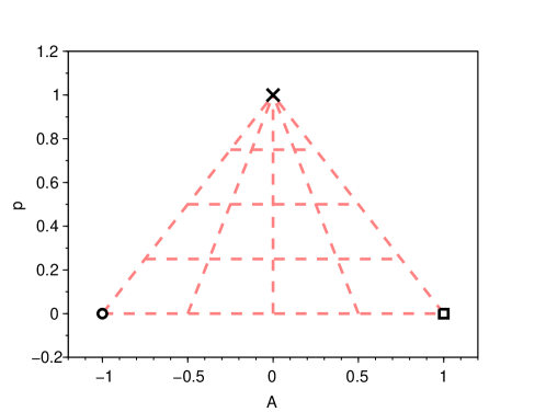
Figure 1: Isotropic Triangle. This figure shows the double Isotropic Index for the states $\rho_{\varphi}$ (square), $\rho_{N\varphi}$ (circle) and $I/2^{n}$ (cross).

III.3.1 Isotropic Triangle properties

Given the invariance of the Isotropic Index with respect to a change of basis, on the following properties we consider the r.s. as $|0\rangle$.

Property 1 (Null probability states).

Considering the projector constructed by the r.s., states with null probability ($Fid(\rho_{0},\rho)=0$), lie at the bottom of the triangle in the interval $\left[-1,-\sqrt{\frac{1}{2^{n}-1}}\right]$.

Proof.

With the decomposition (7), the respective probability is at least $p/(2^{n})$. This implies that for null probability the Isotropic Weight must be $p=0$ and, therefore, $\rho=\hat{\rho}$. Since $Fid\left(\hat{\rho},\rho_{0}\right)=0$ (square root of the probability), in this case we have that $A=-Fid\left(\hat{\rho},\rho_{N0}\right)$. If $\rho=\rho_{N0}\Rightarrow A=-1$. Hence, the states with minimum fidelity with respect to $\rho_{N0}$ and null probability are the $2^{n}-1$ canonical basis states (without $|0\rangle$). Thus,

$$\hat{\rho}=\rho_{i}=|i\rangle\langle i|,\ Fid\left(\hat{\rho},\rho_{N0}\right)=\sqrt{\langle i|\rho_{N0}|i\rangle}=\frac{1}{\sqrt{2^{n}-1}}.$$ (17)

∎

Property 2 (Pure states isotropy).

Let $\rho$ be the density matrix of a pure state of the form $|\psi\rangle=a_{0}|0\rangle+a_{1}e^{i\varphi_{1}}|1\rangle+\dots+a_{2^{n}-1}e^{i\varphi_{2^{n}-1}}|2^{n}-1\rangle$. In this case, it is immediate to see that $p=0$, since there is a unique eigenvalue equal to $1$. Hence, the calculation of $A$ reduces to

$$Fid_{0}=Fid\left(|\psi\rangle,|0\rangle\right)=a_{0},$$ (18)

$$Fid_{N0} = Fid\left(|\psi\rangle,\rho_{N0}\right)=\sqrt{\langle\psi|\rho_{N0}|\psi\rangle},$$ (19)

$$= \sqrt{\sum_{k=1}^{2^{n}-1}\frac{a_{k}^{2}}{2^{n}-1}}=\sqrt{\frac{1-a_{0}^{2}}{2^{n}-1}},$$

$$\Rightarrow A=Fid_{0}-Fid_{N0}=a_{0}-\sqrt{\frac{1-a_{0}^{2}}{2^{n}-1}}.$$ (20)

Therefore, pure states are located in the bottom of the triangle in the interval $\left[-\sqrt{\frac{1}{2^{n}-1}},1\right]$.

Remark.

Since the calculated probability depends only on $a_{0}^{2}$, all pure states with the same probability have the same index.

$$\textit{Iso}_{0}\left(\rho\right)=\left(a_{0}-\sqrt{\frac{1-a_{0}^{2}}{2^{n}-1}},0\right).$$ (21)

Figure 2 illustrates the pure states (black) and the null probability (gray) zones. Note that pure states with null probability have the index in the intersection of both zones, $\textit{Iso}_{0}\left(\rho\right)=\left(-\frac{1}{\sqrt{2^{n}-1}},0\right)$.

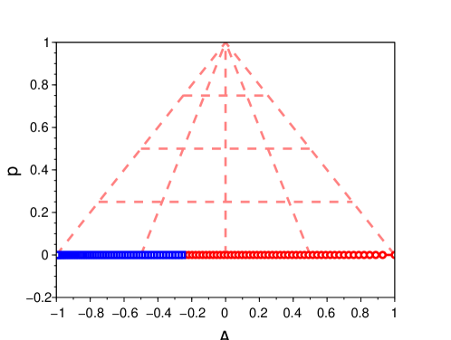
Figure 2: Properties 1 and 2. Pure sates (red circles) and null probability states (blue squares).

Property 3 (Depolarizing channel).

Let $\rho$ be an initial state with a decomposition as in (7) and an index given by $\textit{Iso}_{0}\left(\rho\right)=\left(A,p\right)$. After applying a depolarizing channel operator error Nielsen_2000A the resulting state is

$$\varepsilon\left(\rho\right)=\gamma\frac{I}{2^{n}}+\left(1-\gamma\right)\rho,$$ (22)

with $\gamma\in[0,1]$. In this case

$$\varepsilon\left(\rho\right) = \gamma\frac{I}{2^{n}}+\left(1-\gamma\right)p\frac{I}{2^{n}}+\left(1-\gamma\right)\left(1-p\right)\hat{\rho}$$ (23)

$$= \left(\gamma+p-\gamma p\right)\frac{I}{2^{n}}+\left(1-\gamma-p+\gamma p\right)\hat{\rho}$$

$$= \alpha\frac{I}{2^{n}}+\left(1-\alpha\right)\hat{\rho},$$

being $\alpha$ the new Isotropic Weight. Then $A$ remains constant (same $\hat{\rho}$) and the Isotropic Weight varies from $p$ ($\gamma=0$) to $1$ ($\gamma=1$). As can be seen in figure 3(a), the trajectories are line segments joining the initial state with the maximally mixed state ($\rho=\frac{I}{2^{n}}$).

Property 4 (Unitary evolution).

Due to property 4, for a fixed reference state, if the studied state evolves within a closed system (unitary operator model), the Isotropic Weight remains constant. Figure 3(b) shows the evolution of the index for some initial states.

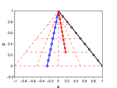
(a) Index evolution due to a depolarizing channel (error probabilities from $0$ to $1$). Initial states: reference state (black circles), null probability state (blue squares) and random state with non-null Isotropic Weight (red crosses).

(b) Index evolution due to random unitary evolution. Initial states: reference state (black circles), random state with $p=0.25$ (blue squares) and random state with $p=0.5$ (red crosses).

Figure 3: Examples for properties 3 and 4, for $4$-qubits states.

Remark.

Even though there is no direct relationship between the probabilities and the Isotropic Alignment, from (11) it can be seen that there is a correlation between the increase (decrease) of the Alignment and the increase (decrease) of such probabilities. This can be observed in figure 4.

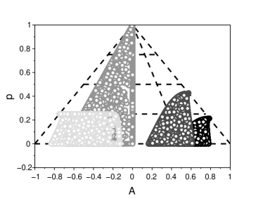
(a) Constant probability zones: $0.8$ (black), $0.6$ (dark gray), $1/2^{n}$ (medium gray) and $0.25/2^{n}$ (light gray).

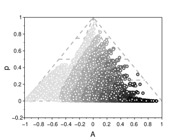
(b) Random states probabilities. Darker zones have higher probabilities.

Figure 4: Isotropic Index for $4$-qubits random states. Probability variation.

IV Horodecki’s isotropic state

An isotropic state Horodecki_1999 is a bipartite $2n$-qubits state, invariant under unitary transformations of the form $U\otimes U^{*}$, being $U$ any unitary matrix and $U^{*}$ its conjugate.

Considering $d=2^{n}$, these states are described by a unique parameter $\alpha$ and are of the form

$$\rho=\left(1-\alpha\right)\frac{I}{d^{2}}+\alpha|\phi\rangle\langle\phi|,\quad-\frac{1}{d^{2}-1}\leq\alpha\leq 1$$ (24)

being

$$|\phi\rangle=\frac{1}{\sqrt{d}}\sum_{j=0}^{2^{n}-1}|j\rangle\otimes|j\rangle$$ (25)

with $|j\rangle$ the canonical basis states of $d$-dimension space.

Unlike an isotropic error state, an isotropic state has, by definition, an even number of qubits. We now calculate the Isotropic Index for isotropic states with reference state $|\phi\rangle$.

If the parameter $\alpha$ is in $[0,1]$, and taking into consideration that $|\phi\rangle$ is a pure state, it is easy to note that the state is already expressed as in decomposition (7). Hence, for this case, the index is $\textit{Iso}_{\varphi}\left(\rho\right)=\left(1,1-\alpha\right)$, i.e. an Isotropic Alignment equal to $1$ and an Isotropic Weight equal to $1-\alpha$. In this particular case of $\alpha$, the state can be seen as applying the depolarizing channel to the original state $|\phi\rangle$.

If, on the other hand, $\alpha$ is in the interval $[-1/(d^{2}-1),0)$, considering $p=1+\left(d^{2}-1\right)\alpha$, the state can be expressed as

$$\rho=\left(1-\alpha\right)\frac{I}{d^{2}}+\alpha|\phi\rangle\langle\phi|=p\,\frac{I}{d^{2}}+\left(1-p\right)\frac{I-|\phi\rangle\langle\phi|}{d^{2}-1}=p\,\frac{I}{d^{2}}+\left(1-p\right)\rho_{N\phi},$$ (26)

where $\rho_{N\phi}$ is the orthogonal isotropic mixed state of state $|\phi\rangle\langle\phi|$. It can be seen that, with the earlier definition, $p$, the Isotropic Weight, is in $[0,1)$ and the Isotropic Alignment is always $-1$.

Hence, an isotropic state can always be interpreted as an isotropic error state with reference state $|\phi\rangle$. Figure 5 shows the evolution of the index in the triangular graph, for $\alpha\in[-1/(d^{2}-1),1]$.

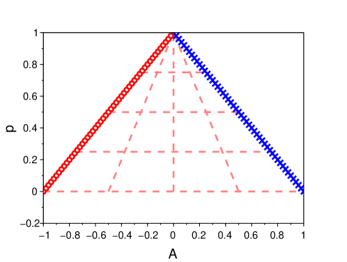
Figure 5: Isotropic Index evolution for isotropic states for: $\alpha\in[0,1]$ (blue crosses) and $\alpha\in[-1/(d^{2}-1),0)$ (red circles).

V Dis-alignment in a Grover’s faulty search

Grover’s quantum search algorithm Grover_1996 ; Grover_2001 deals with the problem of finding a target element in an unstructured database of $N$ elements. It provides a quadratic speedup ($k_{Gr}=\left\lfloor\frac{\pi}{4}\sqrt{N}\right\rfloor$ steps) over the classical brute-force search.

However, considering that any quantum system is subject to error presence, the performance is affected. This phenomena has been studied by several authors in the last years Azuma_2002 ; Chen_2003 ; Shapira_2003 ; Regev_2008 ; Gawron_2012 ; Ambainis_2013_Grover ; Temme_2014 .

In this section, the results obtained in Cohn_2016 are analyzed by using the Isotropic Index.

V.1 Grover’s algorithm

Let there be a set of $N=2^{n}$ quantum basis states in a Hilbert space ($\mathcal{H}=\mathbb{C}^{N}$) in which the search is to be performed, and an unknown marked state (target or solution) among them. Considering a system that identifies the target (oracle), the aim is to find such target using this system in as few steps as possible.

Let $|t\rangle$ be the target element and

$$|s\rangle=\frac{1}{\sqrt{N}}\sum_{i=0}^{N-1}|i\rangle$$ (27)

the initial state. In density matrix representation, these states are $\rho_{t}=|t\rangle\langle t|$ and $\rho_{s}=|s\rangle\langle s|$, respectively. Algorithm 1 describes this search.

1. Set up the superposition state $\rho_{s}$.

2. Apply the oracle operator $O=2\left|t\right\rangle\left\langle t\right|-I$.

3. Apply the diffusion operator $D=2\left|s\right\rangle\left\langle s\right|-I$.

4. Repeat steps 2 and 3 $\left\lfloor\frac{\pi}{4}\sqrt{N}\right\rfloor-1$ times.

5. Perform measurements in the canonical basis in each qubit. The target state will emerge with high probability as $N\gg 1$.

Algorithm 1 Grover’s search algorithm

Applying the algorithm $k$ times results in

$$\rho(k)=|s_{k}\rangle\langle s_{k}|,$$ (28)

with

$$|s_{k}\rangle = \mathrm{sin}\left((2k+1)\theta\right)|t\rangle+\mathrm{cos}((2k+1)\theta)|\bar{t}\rangle,$$

$$|\bar{t}\rangle = \frac{1}{\sqrt{N-1}}\sum_{\begin{subarray}{c}i=0\\ i\neq t\end{subarray}}^{N-1}|i\rangle\ \,\text{and}\ \,\theta=\arcsin\left(\frac{1}{\sqrt{N}}\right).$$ (29)

Therefore, the success probability (of obtaining the target state) after $k$ steps is

$$p(k)=\mathrm{sin}^{2}\left(\left(2k+1\right)\theta\right).$$ (30)

Grover’s operator $G=DO$ can be interpreted as a double reflexion, in the hyperplane generated by the orthogonal states $|t\rangle$ and $|\bar{t}\rangle$, as shown in Figure 6. After $k_{Gr}$ steps, the state is close to $|t\rangle$ ($\theta/2\approx\pi/2$).

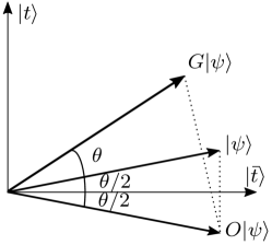
Figure 6: Grover’s algorithm hyperplane generated by $|t\rangle$ and $|\overline{t}\rangle$.

V.2 Local and Total Depolarizing Channels

Salas Salas_2008 and Vrana et al. Vrana_2014 have analyzed the degradation of the algorithm caused by the Total Depolarizing Channel (TDCh). A summary of the results obtained by Cohn et al. Cohn_2016 are presented, in which the degradation of the algorithm with TDCh and Local Depolarizing Channel (LDCh) is compared. Both error models are illustrated in Figure 7.

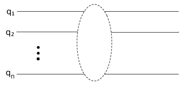
(a) Total Depolarizing Channel error model, TDCh.

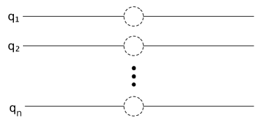
(b) Local Depolarizing Channel error model in each qubit, LDCh.

Figure 7: Depolarizing error models. Errors are applied after each iteration of the algorithm.

The TDCh error $\varepsilon(\rho,\gamma)$, acting on a state $\rho$ with probability $\gamma$, is modeled by Eq. (22). Similarly, the LDCh error is modeled as

$$\varepsilon^{L}(\rho,\alpha)=\varepsilon_{1}(\rho,\alpha)\circ\varepsilon_{2}(\rho,\alpha)\circ\dots\circ\varepsilon_{n}(\rho,\alpha),$$ (31)

being $\alpha$ the error probability per qubit and $\varepsilon_{i}(\rho,\alpha)$ the depolarizing error applied to qubit $i$.

The necessary conditions to maintain the order of the original error-less algorithm are presented in Table 1 for both TDCh ($\gamma$) and LDCh ($\alpha$). As can be seen from the table, LDCh has a more restrictive condition.

TDCh	LDCh
$\gamma\ll(k_{Gr})^{-1}$	$\alpha\ll(k_{Gr}\log_{2}N)^{-1}$

Table 1: Necessary conditions in $\gamma$ (TDCh) and $\alpha$ (LDCh) to maintain Grover’s algorithm original order $\Theta(\sqrt{N})$.

V.3 Isotropic Index interpretation

The Isotropic Index provides a new insight in the analysis of the noisy algorithms evolution. In this case, the error-less state in each $k$ step (V.1) is used as the reference state.

V.3.1 Total Depolarizing Channel

As shown in Cohn_2016 Vrana_2014 , after $k$ steps the state is

$$\rho(k,\gamma)=\left[1-\left(1-\gamma\right)^{k}\right]\frac{I}{2^{n}}+\left(1-\gamma\right)^{k}\rho(k),$$ (32)

where $\rho(k)$ is the error-less density matrix (28) and $\gamma$ is the error probability.

Comparing equations (32) and (7), it is easy to see that the Isotropic Weight is $p=1-\left(1-\gamma\right)^{k}$, and the Isotropic Alignment is always $1$. Figure 8 shows the index evolution for several $\gamma$ values.

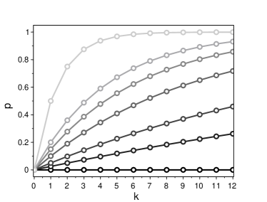
(a) Isotropic Weight evolution versus steps.

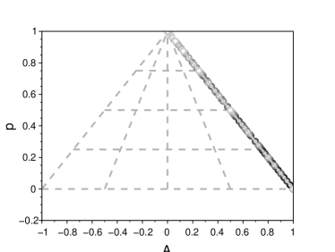
(b) Evolution in the Isotropic Triangle.

Figure 8: Grover’s algorithm with TDCh. Evolutions considering several $\gamma$ values in $\left\{0,0.025,0.05,0.1,0.15,0.2,0.5\right\}$. Darker tones indicate lower error values.

V.3.2 Local Depolarizing Channel

As seen above, Grover’s algorithm is more sensitive to the LDCh error rather than to the TDCh. In the former, even for small values of Isotropic Weight $p$, the Isotropic Alignment has a huge deviation towards $-1$ (i. e. close to $\rho_{N\varphi}$), as illustrated in figure 9. This fact can be interpreted as an indicator of the state deviation from the original hyperplane (figure 6), which affects directly the order.

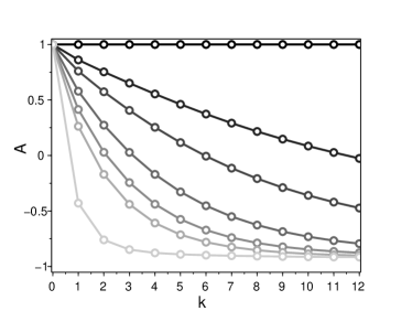
(a) Isotropic Alignment evolution versus steps.

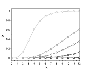
(b) Isotropic Weight evolution versus steps.

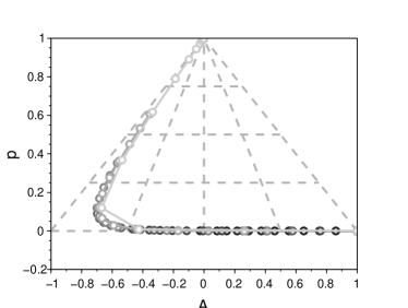
(c) Evolution in the Isotropic Triangle.

Figure 9: Grover’s algorithm with LDCh. Evolutions considering several $\alpha$ values in $\left\{0,0.025,0.05,0.1,0.15,0.2,0.5\right\}$. Darker tones indicate lower error values.

VI Error propagation in Shor’s code

In the last decades, with the purpose of protecting information from errors inherently present in any quantum system, diverse proposals have appeared Calderbank_1996 ; Knill_1998 ; Knill_2000 . Error-correcting codes Laflamme_1996 enabled the development of, among others, fault-tolerant designs Gottesman_1998 ; Aharonov_2008 ; Gottesman_2010 . In this section, we analyze the performance of Shor’s $9$-qubit code Shor_1995 under the effect of the LDCh error using the Isotropic Index.

VI.1 Shor’s code

The $9$-qubit code, proposed by Peter Shor in 1995, is one of the first proposals for quantum error correction. It is capable of correcting any kind of error in any qubit, as long as there is an error present in only one qubit. It does so by combining $3$-qubits codes for both logical and phase errors. The circuit, as illustrated in figure 10, shows a particular unitary implementation that does not need to measure syndrome ancillas.

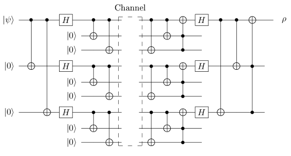
Figure 10: Shor’s code. Encoder/Channel/Decoder&Corrector.

The corresponding logical states are

$$|\psi\rangle=|0\rangle\rightarrow|0_{L}\rangle \equiv \frac{1}{\sqrt{8}}\left(|000\rangle+|111\rangle\right)^{\otimes 3},$$

$$|\psi\rangle=|1\rangle\rightarrow|1_{L}\rangle \equiv \frac{1}{\sqrt{8}}\left(|000\rangle-|111\rangle\right)^{\otimes 3}.$$ (33)

VI.2 Error propagation analysis

In this analysis, we will consider perfect quantum gates and model the error in the channel as a LDCh in each qubit, with $\alpha\in[0,1]$ being the error probability, as in (31). We define the success probability (probability of obtaining the initial state $|\psi\rangle$) as

$$P_{ex}=Fid^{2}\left(|\psi\rangle,\rho\right)=\langle\psi|\rho|\psi\rangle.$$ (34)

It can be seen, figure 11(a), that the states with higher probability are

$$|+\rangle=\frac{|0\rangle+|1\rangle}{\sqrt{2}}\quad\textrm{and}\quad|-\rangle=\frac{|0\rangle-|1\rangle}{\sqrt{2}},$$ (35)

whereas the states with lower probability are

$$|y_{+}\rangle=\frac{|0\rangle+i|1\rangle}{\sqrt{2}}\quad\textrm{and}\quad|y_{-}\rangle=\frac{|0\rangle-i|1\rangle}{\sqrt{2}}.$$ (36)

This result is valid for all $\alpha\in(0,1)$.

Figure 11(b) illustrates the variation of the success probability $P_{ex}$ as a function of error probability $\alpha$ for the initial states $|+\rangle$, $|0\rangle$ and $|y_{+}\rangle$.

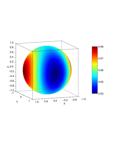
(a) $P_{ex}$ for every initial state $|\psi\rangle$ in Bloch’s sphere. Error probability $\alpha=0.1$.

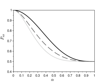
(b) $P_{ex}$ as a function of channel error probability $\alpha$. Solid black curve corresponds to an initial state $|+\rangle$, dashed dark gray to $|0\rangle$ and dotted light gray to $|y_{+}\rangle$.

Figure 11: Success probability $P_{ex}$ for different initial states.

In order to analyze the results using the Isotropic Index, it is necessary to decompose the final state $\rho$ as in equation (7). In this case, success probability $P_{ex}$ is given by

$$P_{ex}=\frac{p}{2}+(1-p)\langle\psi|\hat{\rho}|\psi\rangle,$$ (37)

with $p$ being the Isotropic Weight.

Figure 12 shows the Isotropic Index with initial state

$$|\psi_{\pi/4}\rangle=(1/\sqrt{2})\left(|0\rangle+e^{i\frac{\pi}{4}}|1\rangle\right),$$ (38)

which is the state that has the lowest value of Isotropic Alignment. As can be observed in the figure this value is close to $1$. Hence, for any initial state $|\psi\rangle$, the Isotropic Alignment is always close to $1$. Therefore, by equation (11), the term $\langle\psi|\hat{\rho}|\psi\rangle$ is close to $A^{2}$, and a zero-order approximation yields

$$P_{ex}\approx 1-\frac{p}{2}.$$ (39)

Finally, it is relevant to note that the loss of probability is mainly given by the Isotropic Weight and not by the dis-alignment.

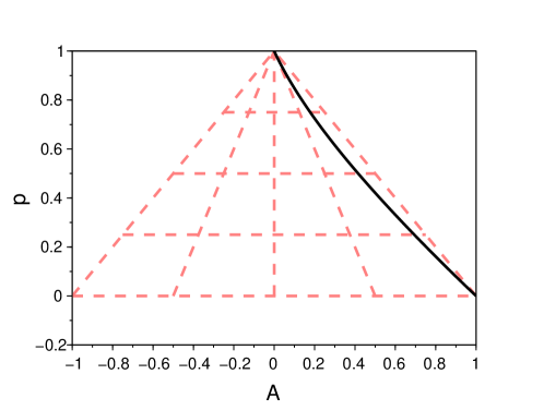
Figure 12: Isotropic Index evolution for $\alpha\in[0,1]$ and initial state $|\psi_{\pi/4}\rangle$.

VII Conclusion

In this paper we introduce an (double) Isotropic Index $Iso(A,p)$ in order to study error propagation in quantum algorithms, given an initial pure reference state. This index characterizes the isotropy using two components: an inherent isotropic component, or Isotropic Weight, $p$ that indicates the maximal mixed $I/2^{n}$ part; and a residual component, that quantified by the Isotropic Alignment indicates the deviation from an actual isotropic error state.

Some examples have been shown in order to explain that degradation due to error propagation may have different origins: some caused by the accumulation of the isotropic component (Shor’s code) and others by the increase of deviation (Grover’s algorithm).

VIII Acknowledgment

A.L.F.O. and E.B. acknowledge financial support from SNI-Uruguay.

References

- [1] T. D. Ladd, F. Jelezko, R. Laflamme, Y. Nakamura, C. Monroe, and J. L. OB́rien. Quantum computers. Nature, 464:45–53, 2010.
- [2] Emanuel Knill, Raymond Laflamme, and Wojciech H. Zurek. Resilient quantum computation: error models and thresholds. Proceedings of the Royal Society of London A: Mathematical, Physical and Engineering Sciences, 454(1969):365–384, 1998.
- [3] D. Gottesman. An introduction to quantum error correction and fault-tolerant quantum computation. In Jr Samuel J. Lomonaco, editor, Quantum Information Science and Its Contributions to Mathematics, Proceedings of Symposia in Applied Mathematics, volume 68, pages 13–60. AMS, 2010.
- [4] Simon J Devitt, William J Munro, and Kae Nemoto. Quantum error correction for beginners. Reports on Progress in Physics, 76(7):076001, 2013.
- [5] Daniel Gottesman. Theory of fault-tolerant quantum computation. Phys. Rev. A, 57:127–137, Jan 1998.
- [6] Dorit Aharonov and Michael Ben-Or. Fault-tolerant quantum computation with constant error rate. SIAM Journal on Computing, 38(4):1207–1282, 2008.
- [7] Michał Horodecki and Paweł Horodecki. Reduction criterion of separability and limits for a class of distillation protocols. Phys. Rev. A, 59:4206–4216, Jun 1999.
- [8] L. K. Grover. Quantum mechanics helps in searching for a needle in haystack. Phys. Rev. Lett., 79(2):325–328, July 1997.
- [9] Peter W. Shor. Scheme for reducing decoherence in quantum computer memory. Phys. Rev. A, 52:R2493–R2496, Oct 1995.
- [10] J. García-López, F. García-Mazarío, and V. Martín. Modelos de error en computación cuántica. Technical Report 20, Universidad Politécnica de Madrid, 2003.
- [11] Jesús García-López and Francisco García Mazarío. Modelos continuos de error en computación cuántica. In Primer Congreso Internacional de Matemáticas en Ingeniería y Arquitectura, Madrid, Spain, 2007. ISBN 978-84-7493-381-9.
- [12] André L. Fonseca de Oliveira, Efrain Buksman, and Jesús García-López. Isotropic double index for quantum errors in one qubit. J. Chem. Chem. Eng., 5(11):1053–1058, November 2011.
- [13] Michel A. Nielsen and Isaac L. Chuang. Quantum computation and quantuminformation. Cambridge University Press, 2000.
- [14] P. S. Bourdon and H. T. Williams. Unital quantum operations on the bloch ball and bloch region. Phys. Rev. A, 69:022314, Feb 2004.
- [15] L. K. Grover. A fast quantum mechanical algorithm for database search. In Proceedings, 28th Annual ACM Symposium on the Theory of Computing p. 212, 1996.
- [16] Lov K. Grover. From Schrödinger’s equation to the quantum search algorithm. American Journal of Physics, 69(7):769–777, 2001.
- [17] Hiroo Azuma. Decoherence in grover’s quantum algorithm: Perturbative approach. Physical Review A, 65:042311, Apr 2002.
- [18] Jingling Chen, Dagomir Kaszlikowski, L.C. Kwek, and C.H. Oh. Searching a database under decoherence. Physics Letters A, 306(5–6):296 – 305, 2003.
- [19] Daniel Shapira, Shay Mozes, and Ofer Biham. Effect of unitary noise on grover’s quantum search algorithm. Physical Review A, 67:042301, Apr 2003.
- [20] Oded Regev and Liron Schiff. Impossibility of a quantum speed-up with a faulty oracle. In Luca Aceto, Ivan Damgård, LeslieAnn Goldberg, MagnúsM. Halldórsson, Anna Ingólfsdóttir, and Igor Walukiewicz, editors, Automata, Languages and Programming, volume 5125 of Lecture Notes in Computer Science, pages 773–781. Springer Berlin Heidelberg, 2008.
- [21] Piotr Gawron, Jerzy Klamka, and Ryszard Winiarczyk. Noise effects in the quantum search algorithm from the viewpoint of computational complexity. Applied Mathematics and Computer Science, 22(2):493–499, 2012.
- [22] Andris Ambainis, Arturs Backurs, Nikolajs Nahimovs, and Alexander Rivosh. Grover’s algorithm with errors. In Antonin Kucera, ThomasA. Henzinger, Jaroslav Nesetril, Tomas Vojnar, and David Antos, editors, Mathematical and Engineering Methods in Computer Science, volume 7721 of Lecture Notes in Computer Science, pages 180–189. Springer Berlin Heidelberg, 2013.
- [23] Kristan Temme. Runtime of unstructured search with a faulty hamiltonian oracle. Physical Review A, 90:022310, Aug 2014.
- [24] Ilan Cohn, André L. Fonseca De Oliveira, Efrain Buksman, and Jesús García López De Lacalle. Grover’s search with local and total depolarizing channel errors: Complexity analysis. International Journal of Quantum Information, 14(02):1650009, 2016.
- [25] P. J. Salas. Noise effect on grover algorithm. The European Physical Journal D, 46(2):365–373, 2008.
- [26] Peter Vrana, David Reeb, Daniel Reitzner, and Michael M. Wolf. Fault-ignorant quantum search. New Journal of Physics, 16:073033, 2014.
- [27] A. R. Calderbank and Peter W. Shor. Good quantum error-correcting codes exist. Phys. Rev. A, 54:1098–1105, Aug 1996.
- [28] Emanuel Knill, Raymond Laflamme, and Lorenza Viola. Theory of quantum error correction for general noise. Phys. Rev. Lett., 84:2525–2528, Mar 2000.
- [29] Raymond Laflamme, Cesar Miquel, Juan Pablo Paz, and Wojciech Hubert Zurek. Perfect quantum error correcting code. Phys. Rev. Lett., 77:198–201, Jul 1996.