A polynomial-time relaxation of the Gromov-Hausdorff distance

Abstract.

The Gromov-Hausdorff distance provides a metric on the set of isometry classes of compact metric spaces. Unfortunately, computing this metric directly is believed to be computationally intractable. Motivated by applications in shape matching and point-cloud comparison, we study a semidefinite programming relaxation of the Gromov-Hausdorff metric. This relaxation can be computed in polynomial time, and somewhat surprisingly is itself a pseudometric. We describe the induced topology on the set of compact metric spaces. Finally, we demonstrate the numerical performance of various algorithms for computing the relaxed distance and apply these algorithms to several relevant data sets. In particular we propose a greedy algorithm for finding the best correspondence between finite metric spaces that can handle hundreds of points.

1. Introduction

In order to study the convergence of sequences of metric spaces, Gromov introduced what is now called the Gromov-Hausdorff metric [Gro81]. Roughly speaking, this metric generalizes the classical Hausdorff distance between subsets of an ambient metric space, to a pair of arbitrary metric spaces by taking the infimum over all embeddings. The Gromov-Hausdorff metric has been of theoretical importance in geometric group theory and is at the heart of the subject of “metric geometry”.

More recently, the Gromov-Hausdorff distance has been proposed as a basic method for comparing point clouds [MS05]. A point cloud is simply a finite metric space (often presented as a subset of $\mathbb{R}^{n}$); this is a fundamental and ubiquitous representation of data. Geometric examples, where the point cloud represents samples from some smooth geometric object, arise from various kinds of shape acquisition devices. Examples with less obvious intrinsic geometric structure are frequently generated by biological data (e.g., collections of gene expression vectors). Given two point clouds, a natural question is to determine if they are related by some isometric transformation; if not, one might wish to know a quantitative measure of their difference.

Another version of this sort of problem is what is known as the point registration problem (also sometimes referred to as point matching and network alignment). Point registration consists in finding a correspondence between point sets or graphs such that a certain cost function is minimized. It appears in computer vision problems like shape matching, computational biology [CK14], and general pattern recognition problems. In some applications, registering or aligning is particularly challenging since there is no explicit correspondence between the sets, often because deformation has occurred or they have different numbers of points. In such cases it is natural to consider a metric on point clouds that is defined in terms of correspondences between point clouds together; the Gromov-Hausdorff distance can be described in terms of a minimax expression over correspondences between the metric spaces, and so is potentially suitable for this purpose.

Unfortunately, exact computation of the Gromov-Hausdorff distance is essentially intractable; it involves the solution of an NP-hard optimization problem. As a consequence, it is natural to consider relaxations. In [Mém11], Mémoli studied a relaxation referred to as the Gromov-Wasserstein distance — this distance is closely related to distances motivated by optimal transport problems [LV09, Stu06], to a “distance distribution” metric defined by Gromov, and also to the cut distance of graphons. Unfortunately, computing the Gromov-Wasserstein distance still requires solving a non-convex optimization problem which does not appear to have attractive performance characteristics in practice.

In this paper, we study a semidefinite programming (SDP) relaxation of the Gromov-Hausdorff distance; this yields a tractable convex optimization problem. We prove that this relaxation defines a pseudometric on point clouds that can be computed in polynomial time. Our pseudometric also provides a relaxed correspondence between point clouds and a lower bound for the Gromov-Hausdorff distance. A similar version of this SDP was recently introduced in [KKBL15] and further studied in [MDK⁺16] and [DL16]; our work provides theoretical validation for some of the computational phenomena observed therein and complements their theoretical framework. We describe the performance of optimized solvers for this SDP. We also propose a non-convex optimization algorithm to approach the registration problem efficiently. The output of this algorithm not only provides a local optimum for the registration problem, but also an upper bound for the Gromov-Hausdorff distance.

2. Background

We begin by recalling the definition of the Gromov-Hausdorff distance; for this, we start with the Hausdorff distance. Let $(Z,d)$ a compact metric space and $\mathcal{C}(Z)$ the collection of all compact sets in $Z$. If $A,B\in\mathcal{C}(Z)$, the Hausdorff distance between $A$ and $B$ can be expressed as

$$d_{\mathcal{H}}^{Z}(A,B)=\inf_{R\in\mathcal{R}(A,B)}\sup_{(a,b)\in R}d(a,b)$$

where $\mathcal{R}(A,B)$ is the set of correspondences in $R\subset A\times B$ such that every element $a\in A$ is related to at least one element in $B$ and every element $b\in B$ is related at least one element in $A$. For many theoretical and practical applications it is common to relax such distance to the Wasserstein distance [Vil03]. In that setting, one endows $\mathcal{C}(Z)$ with a measure,

$$\mathcal{C}_{w}(Z)=\{(A,\mu_{A})\colon A\in\mathcal{C}(Z),\;\operatorname{supp}(\mu_{A})=A\},$$

and relaxes the set of correspondences $\mathcal{R}(A,B)$ to the set of transportation plans

$$\mathcal{M}(\mu_{A},\mu_{B})=\{\mu\colon\mu(A_{0}\times B)=\mu_{A}(A_{0}),\;\mu(A\times B_{0})=\mu_{B}(B_{0}),\text{ for all Borel sets }A_{0}\subset A,\,B_{0}\subset B\}.$$

Then, for $A,B\in\mathcal{C}_{w}(Z)$, the Wasserstein distance is defined for $1\leq p\leq\infty$ as

$$d_{\mathcal{W},p}^{Z}(A,B)=\inf_{\mu\in\mathcal{M}(\mu_{A},\mu_{B})}\left(\int_{A\times B}d^{p}(a,b)d\mu(a,b)\right)^{1/p}\quad\text{for }1\leq p<\infty$$

$$d_{\mathcal{W},\infty}^{Z}(A,B)=\inf_{\mu\in\mathcal{M}(\mu_{A},\mu_{B})}\sup_{(a,b)\in\operatorname{supp}(\mu)}d(a,b).$$

For $A,B$ finite sets this distance can be efficiently computed by a linear program.

The Hausdorff distance suffices to compare metric spaces embedded in a common ambient metric space; Gromov’s idea to extend this to compare arbitrary metric spaces is simply to consider the infimum over all isometric embeddings into a common metric space [Gro01]. Specifically, if $X,Y$ are compact metric spaces, the Gromov-Hausdorff distance is defined as

$$d_{\mathcal{GH}}(X,Y)=\inf_{Z,f,g}d_{\mathcal{H}}^{Z}(f(X),g(Y))$$

where $f\colon X\to Z$ and $g\colon Y\to Z$ are isometric embeddings into $Z$, a metric space. Unfortunately, it is an NP-hard problem to compute this distance.

Since the Hausdorff distance becomes computationally tractable when relaxed to the Wasserstein distance, one might consider a transport-based relaxation of the Gromov-Hausdorff distance that works in the setting of metric measure spaces. In a series of papers [Mém11, Mém07, MS05] Mémoli considers different equivalent expressions for the Gromov-Hausdorff distance, and by relaxing them and considering them in the measure metric space setting, he obtains different gromovizations of the Wasserstein distance, called Gromov-Wasserstein distances. A particularly natural relaxation is based on the observation that the Gromov-Hausdorff distance can be expressed as:

(2.1) $$d_{\mathcal{GH}}(X,Y)=\frac{1}{2}\inf_{R\in\mathcal{R}(X,Y)}\sup_{\begin{subarray}{c}x,x^{\prime}\in X\\ y,y^{\prime}\in Y\\ (x,y),(x^{\prime},y^{\prime})\in R\end{subarray}}\Gamma_{X,Y}(x,y,x^{\prime},y^{\prime})$$

where $\Gamma_{X,Y}(x,y,x^{\prime},y^{\prime})=|d_{X}(x,x^{\prime})-d_{Y}(y,y^{\prime})|$. For $1\leq p\leq\infty$ Mémoli then defines Gromov-Wasserstein relaxations of the Gromov-Hausdorff distance as

(2.2) $$D_{p}(X,Y)=\frac{1}{2}\inf_{\mu\in\mathcal{M}(\mu_{X},\mu_{Y})}\left(\int_{X\times Y}\int_{X\times Y}\left(\Gamma_{X,Y}(x,y,x^{\prime},y^{\prime})\right)^{p}\mu(dx\times dy)\mu(dx^{\prime}\times dy^{\prime})\right)^{1/p}$$

(2.3) $$D_{\infty}(X,Y)=\frac{1}{2}\inf_{\mu\in\mathcal{M}(\mu_{X},\mu_{Y})}\sup_{\begin{subarray}{c}x,x^{\prime}\in X\\ y,y^{\prime}\in Y\\ (x,y),(x^{\prime},y^{\prime})\in\operatorname{supp}(\mu)\end{subarray}}\Gamma_{X,Y}(x,y,x^{\prime},y^{\prime})$$

In his work, Mémoli studies topological properties of the different distance relaxations and how they compare with each other and with the Gromov-Hausdorff distance. He also proposes an algorithm to approximate $D_{p}$, but due the non-convexity of its objective function, no performance guarantees are provided. Recent work [PCS16] has provided efficient heuristic algorithms based on optimal transportation to approximate the Gromov-Wasserstein distance for alignment applications.

Remark 2.4.

Gromov considered another metric on the set of metric measure spaces defined in terms of the convergence of all distance matrix distributions (i.e., the distributions induced by taking the pushforward of the measure to a collection of $n$ points and applying the metric to all pairs). It turns out that this metric is closely related to the Gromov-Wasserstein distance [Stu06, 3.7]. Moreover, these metrics induce the same notion of convergence as arises in the theory of dense graph sequences and graphons. Specifically, we can regard a graph as a metric measure space; the underlying metric space has points the set of vertices and pairwise distances $\frac{1}{2}$ if the points are connected and $1$ otherwise, and the measure assigns equal mass to each point. (See [Ele12] for further discussion of this point).

3. Semidefinite relaxations of Gromov-Wasserstein and Gromov-Hausdorff distances

Consider the setting where $X$ and $Y$ are finite metric spaces (or metric measure spaces), say $X=\{x_{1},\ldots,x_{n}\}$ and $Y=\{y_{1},\ldots,y_{m}\}$ (with measures $\mu_{X}(x_{i})=\nu_{i}$ and $\mu_{Y}(y_{j})=\lambda_{j}$). Let us abbreviate $\Gamma_{X,Y}(x_{i},y_{j},x_{i^{\prime}},y_{j^{\prime}})$ as $\Gamma_{ij,i^{\prime}j^{\prime}}$ for $i,i^{\prime}=1,\ldots,n$ and $j,j^{\prime}=1,\ldots,m$. The formulation of the Gromov-Hausdorff distance given in equation (2.1) can be expressed as a quadratic assignment (Remark 3 in [Mém07]):

(3.1) $$d_{\mathcal{GH}}(X,Y)= \frac{1}{2}\min_{\mu}\max_{ij,i^{\prime}j^{\prime}}\Gamma_{ij,i^{\prime}j^{\prime}}\mu_{ij}\mu_{i^{\prime}j^{\prime}}\quad\text{ subject to }\mu_{ij}\in\{0,1\},\;\;\sum_{j=1}^{m}\mu_{ij}\geq 1,\;\;\sum_{i=1}^{n}\mu_{ij}\geq 1$$

and the expressions (2.2) and (2.3) can be written as (3.2) and (3.3) respectively:

(3.2) $$D_{p}(X,Y)=\frac{1}{2}\min_{\mu\in\mathbb{R}^{n\times m}}\left(\sum_{i,i^{\prime}=1}^{n}\sum_{j,j^{\prime}=1}^{m}\mu_{ij}\mu_{i^{\prime}j^{\prime}}\Gamma_{ij,i^{\prime}j^{\prime}}^{p}\right)^{1/p}\text{subject to }0\leq\mu_{ij}\leq 1,\sum_{i=1}^{n}\mu_{ij}=\lambda_{j},\sum_{j=1}^{m}\mu_{ij}=\nu_{i}$$

(3.3) $$D_{\infty}(X,Y)=\frac{1}{2}\min_{\mu\in\mathbb{R}^{n\times m}}\max_{\stackrel{{\scriptstyle i,i^{\prime},j,j^{\prime}}}{{\mu_{ij}\mu_{i^{\prime}j^{\prime}}\neq 0}}}\Gamma_{ij,i^{\prime}j^{\prime}}\,\text{ subject to }0\leq\mu_{ij}\leq 1,\sum_{i=1}^{n}\mu_{ij}=\lambda_{j},\sum_{j=1}^{m}\mu_{ij}=\nu_{i}$$

In order to approach non-convex optimization problems like (3.1), (3.2) or (3.3), one standard technique is to linearize the objective by lifting $\mu_{ij}\mu_{i^{\prime}j^{\prime}}$ and $\mu_{ij}$ to a symmetric variable $\mathbf{Z}\in R^{nm+1\times nm+1}$ whose entries entries are indexed by pairs $(ij,i^{\prime}j^{\prime})$,$(ij,nm+1)$, $(nm+1,i^{\prime}j^{\prime})$ and $(nm+1,nm+1)$ with $i,i^{\prime}=1,\ldots n$ and $j,j^{\prime}=1,\ldots,m$.

(3.4) $$\mathbf{Z}=\left[\begin{array}[]{c c}\hat{\mathbf{Z}}&\mathbf{z}\\ \mathbf{z}^{\top}&1\end{array}\right].$$

Then note that, for instance, the problems (3.2) and (3.3) are equivalent to problems (3.5) and (3.6) respectively:

(3.5) $$D_{p}(X,Y)=\frac{1}{2}\left(\min_{\mathbf{Z}}\operatorname{Trace}(\Gamma^{(p)}\hat{\mathbf{Z}})\right)^{1/p}\quad\text{ subject to }\mathbf{Z}\in\mathcal{S}$$

(3.6) $$D_{\infty}(X,Y)=\frac{1}{2}\min_{\mathbf{Z}}\max_{i,i^{\prime},j,j^{\prime}\colon\mathbf{Z}\neq 0}\Gamma_{ij,i^{\prime}j^{\prime}}\quad\text{ subject to }\mathbf{Z}\in\mathcal{S}$$

where $\mathcal{S}=\{\mathbf{Z}\in\mathbb{R}^{nm+1\times nm+1}\colon\sum_{i}\mathbf{Z}_{ij,nm+1}=\lambda_{j},\,\sum_{j}\mathbf{Z}_{ij,nm+1}=\nu_{i},\,{\mathbf{Z}}={\mathbf{Z}}^{\top},\,{\mathbf{Z}}\geq 0,\,\operatorname{rank}({\mathbf{Z}})=1\}$ and $\Gamma^{(p)}$ denotes the $p$-th power of the matrix $\Gamma$ entrywise.

The constraint $\operatorname{rank}(\mathbf{Z})=1$ can be relaxed to the convex constraint ${\mathbf{Z}}\succeq 0$ (which means ${\mathbf{Z}}$ is symmetric and positive semidefinite) and additional linear constraints satisfied by the rank 1 matrix can be added to make the relaxation tighter.

Using this recipe we can construct the following family of semidefinite programming relaxations of the Gromov-Wasserstein and Gromov-Hausdorff distances.

(3.7) $$\tilde{d}_{\mathcal{A},p}(X,Y)=\frac{1}{2}\left(\frac{1}{n^{2}}\min_{\mathbf{Z}}\operatorname{Trace}(\Gamma^{(p)}{\hat{\mathbf{Z}}})\right)^{1/p}\quad\text{ subject to }\mathbf{Z}\in\mathcal{A}$$

(3.8) $$\tilde{d}_{\mathcal{A},\infty}(X,Y)=\frac{1}{2}\min_{\mathbf{Z}}\max_{i,j,i^{\prime},j^{\prime}\colon\mathbf{Z}\neq 0}\Gamma_{ij,i^{\prime}j^{\prime}}\quad\text{ subject to }\mathbf{Z}\in{\mathcal{A}}$$

where we can consider different convex sets $\mathcal{A}$ as relaxing to different distances.

1. For a relaxation of the Gromov-Hausdorff distance (or Gromov-Wasserstein for uniform weights $\lambda_{j}=\nu_{i}=1/\max\{n,m\}$ for all $j=1,\ldots,m$ and $i=1,\ldots,n$) consider

   $${\mathcal{A}}=\mathcal{GH}\colon=\{\mathbf{Z}\in\mathbb{R}^{nm+1\times nm+1}\;\colon\quad\sum_{i}{\mathbf{Z}}_{ij,nm+1}\geq 1,\quad\sum_{j}{\mathbf{Z}}_{ij,nm+1}\geq 1,\quad\sum_{i,i^{\prime}}{\mathbf{Z}}_{ij,i^{\prime}j^{\prime}}\geq 1,\;\\ \sum_{j,j^{\prime}}{\mathbf{Z}}_{ij,i^{\prime}j^{\prime}}\geq 1,\quad\mathbf{\hat{Z}1}=\max\{n,m\}\mathbf{z},\quad 0\leq{\mathbf{Z}}\leq 1,\quad{\mathbf{Z}}\succeq 0\}.$$

   Relaxation (3.8) provides a lower bound for the Gromov-Hausdorff distance, since every element of $\mathcal{R}(X,Y)$ induces, up to normalization, a feasible $\mathbf{Z}$. In fact, if the optimal solution of equation (2.1) corresponds to $R\in\mathcal{R}(X,Y)$ such that $(x_{i},y_{j}),(x_{i},y_{j^{\prime}})\in R$ for some $j\neq j^{\prime}$, the solution of equation (3.7) may split the mass in a way so $\mathbf{Z}_{ij,nm+1}+\mathbf{Z}_{ij^{\prime},nm+1}=1$ instead of having $\mathbf{Z}_{ij,nm+1}=\mathbf{Z}_{ij^{\prime},nm+1}=1$.

2. If $|X|=|Y|$ we may want to restrict the set of all correspondences between $X$ and $Y$ (where every element of $X$ is related to at least one element in $Y$ and vice versa) to the set of all bijective correspondences. In that case we can consider a tighter relaxation, that relaxes the registration problem and is similar to the one in [KKBL15].

   $$\mathcal{A}=\operatorname{Reg}\colon=\{\mathbf{Z}\in\mathbb{R}^{n^{2}+1\times n^{2}+1}\colon\displaystyle\sum_{i=1}^{n}{\mathbf{Z}}_{ij,n^{2}+1}=1,\quad\displaystyle\sum_{j=1}^{n}{\mathbf{Z}}_{ij,n^{2}+1}=1,\quad\mathbf{Z}_{n^{2}+1,n^{2}+1}=1,\\ \displaystyle\sum_{i,i^{\prime}=1}^{n}\mathbf{Z}_{ij,i^{\prime}j^{\prime}}=1,\quad\displaystyle\sum_{j,j^{\prime}=1}^{n}\mathbf{Z}_{ij,i^{\prime}j^{\prime}}=1,\quad\mathbf{Z}_{ij,ij^{\prime}}=0\text{ if }j\neq j^{\prime},\quad\mathbf{Z}_{ij,ij^{\prime}}=0\text{ if }i\neq i^{\prime},\\ \operatorname{Trace}({\mathbf{Z}})=n+1,\quad\mathbf{\hat{Z}1}=n\mathbf{z},\quad 0\leq{\mathbf{Z}}\leq 1,\quad\mathbf{Z}\succeq 0\}$$

3. The registration relaxation can be extended to finite metric spaces with different numbers of points. Let as before $|X|=n$ and $|Y|=m$. First, without loss of generality assume that $n\geq m$. Now consider the problem (2.1) where the set $\mathcal{R}(X,Y)$ is restricted to surjective functions $X\to Y$. Then relax the feasible set to the convex set:

   $$\mathcal{A}=\operatorname{Sur}\colon=\{\mathbf{Z}\in\mathbb{R}^{nm+1\times nm+1}\colon\displaystyle\sum_{i=1}^{n}{\mathbf{Z}}_{ij,nm+1}\geq 1,\quad\displaystyle\sum_{j=1}^{m}{\mathbf{Z}}_{ij,nm+1}=1,\quad\mathbf{Z}_{nm+1,nm+1}=1,\\ \displaystyle\sum_{i,i^{\prime}=1}^{n}\mathbf{Z}_{ij,i^{\prime}j^{\prime}}\geq 1,\quad\displaystyle\sum_{j,j^{\prime}=1}^{m}\mathbf{Z}_{ij,i^{\prime}j^{\prime}}=1,\quad\mathbf{Z}_{ij,ij^{\prime}}=0\text{ if }j\neq j^{\prime},\\ \operatorname{Trace}({\mathbf{Z}})=n+1,\quad\mathbf{\hat{Z}1}=n\mathbf{z},\quad 0\leq{\mathbf{Z}}\leq 1,\;\;\mathbf{Z}\succeq 0,\}$$

   Note that the set of constraints assumes that $i,i^{\prime}=1,\ldots n$, $j,j^{\prime}=1,\ldots m$ and $n\geq m$ and it is not symmetric with respect to $i$ and $j$. Also note that under this relaxation, there exist sets that $d_{\mathcal{GH}}(X,Y)=0$ but the relaxed distance (3.7) with $\mathcal{A}=\operatorname{Sur}$ satisfies $\tilde{d}_{\operatorname{Sur},p}(X,Y)\neq 0$ (and the same phenomena occurs for $\mathcal{A}=\operatorname{Reg}$). For instance $X=\{x,x,y\}$ and $Y=\{x,y,y\}$. This is an artifact of only allowing surjective functions instead of all possible relations in $\mathcal{R}(X,Y)$.

Remark 3.9.

Even though the $\max$ objective in equation (3.8) is convex, it is not smooth, which we observe to significantly hurt the performance of the numerical implementations. This is one reason to consider the $p$-norm approach to this relaxation and define the family of SDP relaxations (3.7) for $1\leq p<\infty$.

Remark 3.10.

Note that linear constraints in the sets $\mathcal{A}$ are not linearly independent and the extra variable $\mathbf{z}$ is redundant. However, one can easily choose alternative sets of constraints (even with fewer constraints or where the extra constraint is not redundant) with the same objectives in mind: (i) the relaxation is tight when the spaces are isometric (ii) the corresponding objective value satisfies the triangle inequality when $|X|=|Y|$.

We are primarily interested in the semidefinite programming relaxations of the Gromov-Hausdorff distance for finite metric spaces, namely $\tilde{d}_{\mathcal{A},p}$, $1\leq p\leq\infty$ for $\mathcal{A}=\mathcal{GH},\operatorname{Reg},\operatorname{Sur}$. In figure 1, we extend a diagram of Mémoli’s to situate the SDP relaxations we study in this paper.

Figure 1. Here $\mathcal{G}$ is the collection of all compact metric spaces and $\mathcal{G}_{w}$ the collection of all metric measure spaces. The horizontal arrows represent the relaxation on the notion of correspondences. The gromovization arrows represent the process of getting rid of the ambient space.

4. Topological properties of the relaxed distances

In this section, we prove the main theoretical results of the paper. We begin by showing that the distances obtained by semidefinite relaxation are in fact pseudometrics on suitable subsets of the set of isometry classes of finite metric spaces; i.e., these distances satisfy all the axioms for a metric except that there exist distinct finite metric spaces such that the relaxed distance between them is $0$. We then study various properties of the induced topology, proving analogues of the standard results about the topology induced on the set of isometry classes of compact metric spaces by the Gromov-Hausdorff distance.

4.1. Pseudometrics

Let $\mathcal{G}_{<\infty}$ the set of all finite metric spaces. First, we observe that $\tilde{d}_{\mathcal{A},\infty}$ is a pseudometric in $\mathcal{G}_{<\infty}$. However, if the spaces $X,Y,Z$ have different numbers of points we cannot expect the triangle inequality to hold for $\tilde{d}_{\mathcal{A},p}$. That is because the triangle inequality does not even hold for tight solutions of equation (3.7) (i.e., rank 1 solutions, corresponding to elements of $\mathcal{R}(X,Y)$). This is an artifact of replacing the $\max$ with a sum.

In order to illustrate that fact we consider a simple example. Let $d_{\mathcal{GH},1}$ be the optimal of (3.7) for $p=1$ and $\mathcal{A}$ the domain of (3.1) (i.e. the solutions corresponding to elements of $\mathcal{R}(X,Y)$ ). Then consider $X=\{x,y\}$, $Y=\{x,x,y\}$, $Z=\{y\}$, and observe that triangle inequality is not satisfied since $d_{\mathcal{GH},1}(X,Y)=0$, $d_{\mathcal{GH},1}(Y,Z)=2d(x,y)$ and $d_{\mathcal{GH},1}(X,Z)=d(x,y)$.

Nonetheless, if we consider the set of metric spaces with $n$ points, which we denote by $\mathcal{G}_{n}$, we will show that $\tilde{d}_{\mathcal{A},p}$ for $1\leq p<\infty$ is a pseudometric on $\mathcal{G}_{n}$. The most interesting part of this verification is the triangle inequality, which we prove in Theorem 4.5 below. In contrast to the situation with the Gromov-Hausdorff distance, passing to isometry classes of finite metric spaces does not suffice to produce an actual metric. Of course, if $X$ and $Y$ are isometric spaces then $\tilde{d}_{\mathcal{A},p}(X,Y)=0$. By construction $\tilde{d}_{\mathcal{A},p}(\cdot,\cdot)\geq 0$ and the isometry between $X$ and $Y$ induces a feasible solution for equation (3.7) with objective value 0. However, there exists non-isometric spaces $X,Y$ such that $\tilde{d}_{\mathcal{A},p}(X,Y)=0$. Examples of that phenomenon can be constructed by observing that the graph isomorphism problem can be reduced to deciding whether the Gromov-Hausdorff distance is zero. Given a graph $G=(V,E)$ one then constructs a metric space $X(G)$ where

(4.1) $$d(v,v^{\prime})=\left\{\begin{matrix}1&\text{if }(v,v^{\prime})\in E\\ K\gg|V|&\text{otherwise}.\end{matrix}\right.$$

Therefore, given two graphs $G,G^{\prime}$ we have that $G,G^{\prime}$ are isomorphic if and only if $d_{\mathcal{GH}}(X(G),X(G^{\prime}))=0$. There exist explicit examples in the literature of graphs where any SDP relaxation on $|V|^{2}\times|V|^{2}$ matrices cannot distinguish between two non-isomorphic graphs [OWWZ14]. For such examples, $\tilde{d}_{\mathcal{A},p}(X(G),X(G^{\prime}))=0$ (see Figure 2).

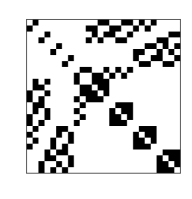
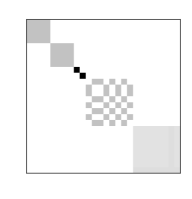
Figure 2. We consider 3XOR instances with 5 variables and 4 equations and we construct the reduction from 3XOR to graph isomorphism from [OWWZ14]. The left and middle figures represent corresponding adjacency graphs obtained after the reduction from the following system of equations in $\mathbb{Z}_{2}$:
$\quad\quad\left.\begin{matrix}x_{1}\oplus x_{2}\oplus x_{5}=b_{1}\\ x_{1}\oplus x_{2}\oplus x_{5}=b_{2}\\ x_{1}\oplus x_{3}\oplus x_{4}=b_{3}\\ x_{2}\oplus x_{3}\oplus x_{4}=b_{4}\end{matrix}\right.,\text{ with }\left(\begin{matrix}b_{1}\\ b_{2}\\ b_{3}\\ b_{4}\end{matrix}\right)=\left(\begin{matrix}1\\ 1\\ 0\\ 1\end{matrix}\right)\text{(left), and }\left(\begin{matrix}b_{1}\\ b_{2}\\ b_{3}\\ b_{4}\end{matrix}\right)=\left(\begin{matrix}0\\ 0\\ 0\\ 0\end{matrix}\right)\text{ (middle).}$
Each graph has 26 vertices. We construct finite metric spaces $X$ and $Y$ according to (4.1) and we use SDPNAL+ [YST15] to compute the the relaxed distance, obtaining $\tilde{d}_{\operatorname{Reg},1}(X,Y)=0$. The minimizer $\mathbf{Z}$ of (3.7) is rank 16. The figure in the right shows a soft assignment between $X$ and $Y$ obtained from $\mathbf{Z}$ by computing $\hat{\mathbf{Z}}\mathbf{1}$ and rearranging accordingly.

Theorem 4.2.

Consider $\tilde{d}_{\mathcal{A},p}$ and $\tilde{d}_{\mathcal{A},\infty}$ defined in equations (3.7) and (3.8) respectively for $\mathcal{A}=\mathcal{GH},\operatorname{Reg},\operatorname{Sur}$. Then we have:

1. For $X,Y,W\in\mathcal{G}_{n}$, and $1\leq p<\infty$, $\tilde{d}_{\mathcal{A},p}$ satisfies the triangle inequality.

2. For $X,Y,W\in\mathcal{G}_{<\infty}$, $\tilde{d}_{\mathcal{A},\infty}$ satisfies the triangle inequality.

Proof.

We begin by proving part (a). Note that it suffices to show that for $p\geq 1$,

(4.3) $$\tilde{d}_{\mathcal{A},p}(X,W)^{p}\leq\tilde{d}_{\mathcal{A},p}(X,Y)^{p}+\tilde{d}_{\mathcal{A},p}(Y,W)^{p}.$$

This follows from the fact that for $a,b>0$ and $p\geq 1$ we have $a^{p}+b^{p}\leq(a+b)^{p}$ and therefore if equation (4.3) holds we have:

$$\tilde{d}_{\mathcal{A},p}(X,W)\leq\sqrt[p]{\tilde{d}_{\mathcal{A},p}(X,Y)^{p}+\tilde{d}_{\mathcal{A},p}(Y,W)^{p}}\leq\tilde{d}_{\mathcal{A},p}(X,Y)+\tilde{d}_{\mathcal{A},p}(Y,W).$$

Now let $\mathbf{Z}$ and $\mathbf{V}$ the minimizers in equation (3.7) for $X,Y$ and $Y,W$ respectively in $\mathcal{A}$. From $\mathbf{Z}$ and $\mathbf{V}$ we construct $\mathbf{T}$ feasible for $X,W$ in equation (3.7) and we show the objective function in $\mathbf{T}$ is smaller or equal to $\tilde{d}_{\mathcal{A},p}(X,Y)+\tilde{d}_{\mathcal{A},p}(Y,W)$.

If $x_{i},x_{i^{\prime}}\in X$, $y_{j},y_{j^{\prime}}\in Y$ and $w_{k},w_{k^{\prime}}\in W$ let $\mathbf{T}$ the unique feasible matrix in $\mathcal{A}$ that satisfies

(4.4) $$\hat{\mathbf{T}}_{ik,i^{\prime}k^{\prime}}\colon=\sum_{j,j^{\prime}}\hat{\mathbf{Z}}_{ij,i^{\prime}j^{\prime}}\hat{\mathbf{V}}_{jk,j^{\prime}k^{\prime}}.$$

To see that $\mathbf{T}$ is well-defined, observe that it is straightforward to check that $\mathbf{T}$ satisfies the linear and inequality constraints of $\mathcal{A}$ using the fact that $\mathbf{Z}$ and $\mathbf{V}$ belong to $\mathcal{A}$. In order to verify that $\mathbf{T}$ is positive semidefinite, consider the Cholesky decompositions of $\mathbf{Z}$ and $\mathbf{V}$. Then

$$\hat{\mathbf{Z}}_{ij,i^{\prime}j^{\prime}}=z_{ij}^{\top}z_{i^{\prime}j^{\prime}},\quad\hat{\mathbf{V}}_{jk,j^{\prime}k^{\prime}}=v_{jk}^{\top}v_{j^{\prime}k^{\prime}}$$

where $z$ and $v$ do not necessarily correspond to the last column in equation (3.4). In fact $z$ is a $r\times n^{2}$ matrix where $r$ is the rank of $\hat{\mathbf{Z}}$ and $z_{ij}$ is the column of $z$ indexed by $i=1,\ldots,n$ and $j=1,\ldots,n$. Then note

$$\hat{\mathbf{T}}_{ik,i^{\prime}k^{\prime}}=\sum_{j,j^{\prime}}\hat{\mathbf{Z}}_{ij,i^{\prime}j^{\prime}}\hat{\mathbf{V}}_{jk,j^{\prime}k^{\prime}}=\left\langle\sum_{j}z_{ij}\otimes v_{jk},\sum_{j^{\prime}}z_{i^{\prime}j^{\prime}}\otimes v_{j^{\prime}k^{\prime}}\right\rangle$$

therefore $\hat{\mathbf{T}}$ is PSD since it is a Gram matrix, and $\mathbf{T}$ is PSD since it has the same rank as $\hat{\mathbf{T}}$.

For the triangle inequality we need to show

(4.5) $$\sum_{i,i^{\prime}}\sum_{k,k^{\prime}}\mathbf{T}_{ik,i^{\prime}k^{\prime}}|d_{X}(x_{i},x_{i^{\prime}})-d_{W}(w_{k},w_{k^{\prime}})|\leq\sum_{i,i^{\prime}}\sum_{j,j^{\prime}}\mathbf{Z}_{ij,i^{\prime}j^{\prime}}|d_{X}(x_{i},x_{i^{\prime}})-d_{Y}(y_{j},y_{j^{\prime}})|\\ +\sum_{j,j^{\prime}}\sum_{k,k^{\prime}}\mathbf{V}_{jk,j^{\prime}k^{\prime}}|d_{X}(x_{j},x_{j^{\prime}})-d_{W}(w_{k},w_{k^{\prime}})|.$$

In the case we are dealing with, where $|X|=|Y|=|W|$, the constraints

$$\sum_{i,i^{\prime}}\mathbf{Z}_{ij,i^{\prime}j^{\prime}}\geq 1\qquad\textrm{and}\qquad\sum_{k,k^{\prime}}\mathbf{V}_{jk,j^{\prime}k^{\prime}}\geq 1$$

are tight, meaning that equality holds, so for all $j,j^{\prime}$, we can multiply by 1 and rewrite the RHS of equation (4.5) as

$$\sum_{i,i^{\prime}}\sum_{j,j^{\prime}}\mathbf{Z}_{ij,i^{\prime}j^{\prime}}|d_{X}(x_{i},x_{i^{\prime}})-d_{Y}(y_{j},y_{j^{\prime}})|\sum_{k,k^{\prime}}\mathbf{V}_{jk,j^{\prime}k^{\prime}}+\sum_{j,j^{\prime}}\sum_{k,k^{\prime}}\mathbf{V}_{jk,j^{\prime}k^{\prime}}|d_{X}(x_{j},x_{j^{\prime}})-d_{W}(w_{k},w_{k^{\prime}})|\sum_{i,i^{\prime}}\mathbf{Z}_{ij,i^{\prime}j^{\prime}}$$

$$=\sum_{i,i^{\prime}}\sum_{k,k^{\prime}}\sum_{j,j^{\prime}}\mathbf{Z}_{ij,i^{\prime}j^{\prime}}\mathbf{V}_{jk,j^{\prime}k^{\prime}}(|d_{X}(x_{i},x_{i^{\prime}})-d_{Y}(y_{j},y_{j^{\prime}})|+|d_{Y}(y_{j},y_{j^{\prime}})-d_{W}(w_{k},w_{k^{\prime}})|)$$

Now it is clear that equation (4.5) follows from the triangle inequality in $\mathbb{R}$, which completes the verification of part (a).

In order to prove part (b), now we let $X,Y,Z$ to be finite metric spaces with arbitrary number of points. And we let $\mathbf{Z}$ and $\mathbf{V}$ the minimizers in equations (3.8) for $X,Y$ and $Y,W$ respectively as before. We define $\mathbf{T}$ as in equation (4.4). We know $\mathbf{T}$ is feasible for equation (3.8) so the remaining step to prove is

(4.6) $$\max_{\mathbf{T}\neq 0}\Gamma_{ik,i^{\prime}k^{\prime}}\leq\max_{\mathbf{Z}\neq 0}\Gamma_{ij,i^{\prime}j^{\prime}}+\max_{\mathbf{V}\neq 0}\Gamma_{jk,j^{\prime}k^{\prime}}$$

Let $(ik,i^{\prime}k^{\prime})$ the $\arg\max$ of the left hand side of equation (4.6). Since ${\mathbf{T}}_{ik,i^{\prime}k^{\prime}}\neq 0$ and ${\mathbf{T}}_{ik,i^{\prime}k^{\prime}}=\sum_{j,j^{\prime}}{\mathbf{Z}}_{ij,i^{\prime}j^{\prime}}{\mathbf{T}}_{kj,k^{\prime}j^{\prime}}$ then there exists $j,j^{\prime}$ such that ${\mathbf{Z}}_{ij,i^{\prime}j^{\prime}}\neq 0$ and ${\mathbf{T}}_{kj,k^{\prime}j^{\prime}}\neq 0$. Then we have

(4.7) $$\tilde{d}_{\mathcal{A},\infty}(X,W)\leq\max_{\mathbf{T}\neq 0}\Gamma_{ik,i^{\prime}k^{\prime}}=|d_{X}(x_{i},x_{i^{\prime}})-d_{W}(w_{k},w_{k^{\prime}})|\\ \leq|d_{X}(x_{i},x_{i^{\prime}})-d_{Y}(y_{j},y_{j^{\prime}})|+|d_{Y}(y_{j},y_{j^{\prime}})-d_{W}(w_{k},w_{k^{\prime}})|\leq\max_{\mathbf{Z}\neq 0}\Gamma_{ij,i^{\prime}j^{\prime}}+\max_{\mathbf{V}\neq 0}\Gamma_{jk,j^{\prime}k^{\prime}}\\ =\tilde{d}_{\mathcal{A},\infty}(X,Y)+\tilde{d}_{\mathcal{A},\infty}(Y,W).$$

∎

Remark 4.8.

The same argument will show that $\tilde{d}_{\mathcal{GW},p}$ satisfies triangle inequality as long as we add the constraint $\hat{\mathbf{Z}}\mathbf{1}=n\mathbf{z}$, where $n=|X|=|Y|=|W|$ and the measure of each of the points is equal $1/n$.

4.2. Monotonicity and continuity properties

The following lemma shows the monotonicity of $\tilde{d}_{\mathcal{A},p}$ with respect to $p$. The second part of the lemma proves continuity of $\tilde{d}_{\mathcal{A},p}$ at infinity.

Proposition 4.9.

For any $X$,$Y$ finite metric spaces we have:

1. If $1\leq p\leq q<\infty$ then $\tilde{d}_{\mathcal{A},p}(X,Y)\leq\tilde{d}_{\mathcal{A},q}(X,Y)\leq\tilde{d}_{\mathcal{A},\infty}(X,Y)$.

2. $\lim_{p\to\infty}\tilde{d}_{\mathcal{A},p}(X,Y)=\displaystyle\min_{\mathbf{Z}\in\mathcal{\tilde{T}}}\max_{i,j,i^{\prime},j^{\prime}\colon\mathbf{Z}\neq 0}\Gamma_{ij,i^{\prime}j^{\prime}}=\tilde{d}_{\mathcal{A},\infty}(X,Y)$.

Proof.

Let $\mathbf{Z}\in{\mathcal{A}}$ optimal for equations (3.8) or (3.7) for some value of $p$. Then $\mathbf{1^{\top}\hat{Z}1}=n^{2}$. The weighted power mean inequality implies

$$\left(\frac{1}{n^{2}}\sum_{ij,i^{\prime}j^{\prime}}\Gamma_{ij,i^{\prime}j^{\prime}}^{p}\mathbf{Z}_{ij,i^{\prime}j^{\prime}}\right)^{1/p}\leq\left(\frac{1}{n^{2}}\sum_{ij,i^{\prime}j^{\prime}}\Gamma_{ij,i^{\prime}j^{\prime}}^{q}\mathbf{Z}_{ij,i^{\prime}j^{\prime}}\right)^{1/q}\leq\max_{i,j,i^{\prime},j^{\prime}\colon\mathbf{Z}_{ij,i^{\prime}j^{\prime}}\neq 0}\Gamma_{ij,i^{\prime}j^{\prime}}$$

and taking the infimum in $\mathbf{Z}$ we obtain (a).

Now for fixed $\mathbf{Z}$ let $\Gamma_{\mathbf{Z}}^{*}=\max\{\Gamma_{ij,i^{\prime}j^{\prime}}\colon\mathbf{Z}_{ij,i^{\prime}j^{\prime}}\neq 0\}$, then using the standard calculus argument

$$\lim_{p\to\infty}\left(\frac{1}{n^{2}}\sum_{ij,i^{\prime}j^{\prime}}\Gamma_{ij,i^{\prime}j^{\prime}}^{p}\mathbf{Z}_{ij,i^{\prime}j^{\prime}}\right)^{1/p}=\Gamma^{*}_{\mathbf{Z}}\lim_{p\to\infty}\left(\sum_{ij,i^{\prime}j^{\prime}}\left(\frac{\Gamma_{ij,i^{\prime}j^{\prime}}}{\Gamma^{*}_{\mathbf{Z}}}\right)^{p}\frac{\mathbf{Z}_{ij,i^{\prime}j^{\prime}}}{n^{2}}\right)^{1/p}=\Gamma^{*}_{\mathbf{Z}}.$$

and taking infimum in $\mathbf{Z}$ we obtain (b). ∎

Proposition 4.9 holds for metric spaces $X$ and $Y$ with possibly different number of points and it says that even though $\tilde{d}_{\mathcal{A},p}$ may not satisfy the triangle inequality, it does in the limit $p\to\infty$.

4.3. Extension of the distance to compact infinite sets

Every compact metric space $X$ is the limit of a sequence of finite metric spaces in the Gromov-Hausdorff topology, denoted here by $\tau_{\mathcal{GH}}$ (see for instance [BBI01, Example 7.4.9]). In fact, by taking $\epsilon_{n}\to 0$ and choosing a finite $\epsilon_{n}$-net $S_{n}$ in $X$ for every $n$, we get $S_{n}\stackrel{{\scriptstyle\mathcal{GH}}}{{\to}}X$ because

$$d_{\mathcal{GH}}(X,Sn)\leq d_{\mathcal{H}}(X,S_{n})\leq\epsilon_{n}.$$

This property inspires the following definition of an actual distance between compact metric spaces.

Definition 4.10.

Let $X,Y$ compact metric spaces. Given $\epsilon_{n}\to 0$, let $X_{n},Y_{n}$ respective $\epsilon_{n}$-nets of $X$ and $Y$, with the same number of points $N$. Define

(4.11) $$\hat{d}_{\mathcal{A},p}(X,Y)=\inf_{\epsilon_{n},\;X_{n}\,Y_{n}}\lim\sup_{n\to\infty}\tilde{d}_{\mathcal{A},p}(X_{n},Y_{n})$$

Note that $\lim\sup$ exists because $\tilde{d}_{\mathcal{A},p}(X_{n},Y_{n})\leq\tilde{d}_{\mathcal{A},\infty}(X_{n},Y_{n})\leq\frac{1}{2}\max(\operatorname{diam}(X),\operatorname{diam}(Y))$ for all $n$. Also, note the triangle inequality holds for this limit, which also implies that $\hat{d}_{\mathcal{A},p}$ and $\tilde{d}_{\mathcal{A},p}$ may not agree.

To illustrate how the right hand side of (4.11) behaves, let’s say that $|X|<|Y|$ and for some $n$ the $\epsilon_{n}$-net $Y_{n}$ of $Y$ has at least $N$ points and $|X|<N$, then consider $X_{n}$ to be $X$ with some repeated points and run the SDP (3.7) or (3.8) to compute $\tilde{d}_{\mathcal{A},p}(X_{n},Y_{n})$ so that $|Y_{n}|=|X_{n}|=N$. Note that this is well defined and when $\tilde{d}_{\mathcal{A},p}(X_{n},X)$ exists (i.e. $\mathcal{A}=\mathcal{GH},\operatorname{Sur}$) we have $\tilde{d}_{\mathcal{A},p}(X_{n},X)=0$ because the matrix $\mathbf{Z}$ corresponding to the surjective function $X_{n}\to X$ is in $\mathcal{A}$ and has objective value 0.

4.4. Comparison with the Gromov-Hausdorff distance

Let $\mathcal{X}$ denote the set of isometry classes of compact metric spaces. Definition 4.10 extends the relaxed distances (3.7) and (3.8) to $\mathcal{X}$, obtaining the function $\hat{d}_{\mathcal{A},p}\colon\mathcal{X}\times\mathcal{X}\to\mathbb{R}$.

Lemma 4.12.

For $X,Y\in\mathcal{X}$ we have for $1\leq p\leq\infty$

$$\hat{d}_{A,p}(X,Y)\leq d_{\mathcal{GH}}(X,Y)$$

Proof.

First assume $X,Y$ are finite and let $R\in\mathcal{R}(X,Y)$ the minimizer in (2.1). If $|R|=N$ let $X_{N},Y_{N}$ the $\epsilon$-net so that every element of $X$ appears in $X_{N}$ as many times as it appears in $R$ (and the same for $Y_{N}$). Then the bijective function between $X_{N}$ and $Y_{N}$ corresponding to $R$ induces a feasible $\mathbf{Z}$, proving the result in the finite case. For the remaining case consider a $\epsilon_{n}$-net where $\epsilon_{n}\to 0$. ∎

Now consider $X,Y$ finite metric spaces. First observe that $\mathcal{A}=\mathcal{GH}$ includes the $\mathbf{Z}$ induced by all elements in $\mathcal{R}(X,Y)$, which together with Proposition 4.9 implies

$$\tilde{d}_{\mathcal{GH},p}(X,Y)\leq\tilde{d}_{\mathcal{GH},\infty}(X,Y)\leq d_{\mathcal{GH}}(X,Y).$$

Since $\operatorname{Sur}\subset\mathcal{G}H$ we have

$$\tilde{d}_{\mathcal{GH},p}(X,Y)\leq\tilde{d}_{\operatorname{Sur},p}(X,Y),$$

and if $|X|=|Y|$ we can consider that $\operatorname{Reg}\subset\operatorname{Sur}$ therefore

$$\tilde{d}_{\mathcal{GH},p}(X,Y)\leq\tilde{d}_{\operatorname{Sur},p}(X,Y)\leq\tilde{d}_{\operatorname{Reg},p}(X,Y).$$

Also, the smaller the set $\mathcal{A}$, the more likely is the relaxation to produce a tight solution (a rank 1 solution, corresponding with an element of $\mathcal{R}(X,Y)$). Note that neither $\tilde{d}_{\operatorname{Sur},p}$ nor $\tilde{d}_{\operatorname{Reg},p}$ are comparable with $d_{\mathcal{GH}}$.

4.5. Topologies induced by relaxed distances

Any metric or pseudometric $d$ defines a topology $\tau$ characterized by the property that given a sequence $X_{n}$, we have convergence $X_{n}\stackrel{{\scriptstyle\tau}}{{\to}}X$ if and only if $d(X_{n},X)\to 0$. In particular, the Gromov-Hausdorff distance induces a topology on the set of isometry classes of compact metric spaces. The Gromov-Hausdorff topology is a fairly weak topology; for example, there are many compact sets. Proposition 7.4.12 in [BBI01] characterizes the Gromov-Hausdorff convergence in terms of $\epsilon$-nets, implying that if a sequence $\{X_{n}\}$ converges in the Gromov-Hausdorff topology, then for all $\epsilon>0$, the cardinality of $\epsilon$-nets is uniformly bounded over $X_{n}$. Therefore if a class $\mathcal{X}$ of metric spaces is pre-compact (i.e. any sequence of elements of $\mathcal{X}$ has a convergent subsequence) in the Gromov-Hausdorff topology, then for every $\epsilon>0$ the size of a minimal $\epsilon$-net is uniformly bounded over all elements of $\mathcal{X}$. The analysis in [BBI01] shows that this property of $\mathcal{X}$, along with the fact that the diameters of its members are uniformly bounded (what is called totally boundedness, Definition 4.14), is sufficient for pre-compactness (Theorem 4.15).

Let $\hat{\tau}_{\mathcal{A},p}$ ($1\leq p\leq\infty$), and $\tilde{\tau}_{\mathcal{A},\infty}$ denote the topologies induced by the pseudometrics $\hat{d}_{\mathcal{A},p}$ ($1\leq p\leq\infty$) and $\tilde{d}_{\mathcal{A},\infty}$, respectively. We obtain an analogous characterization of pre-compact sets in the topology for $\hat{\tau}_{\mathcal{A},p}$ for $1\leq p\leq\infty$ in Corollary 4.16 below.

Proposition 4.13.

[BBI01, 7.4.12] For compact metric spaces $X$ and $\{X_{n}\}_{n=1}^{\infty}$, $X_{n}\stackrel{{\scriptstyle\tau_{\mathcal{GH}}}}{{\longrightarrow}}X$ if and only if the following holds. For every $\epsilon>0$ there exist a finite $\epsilon$-net $S$ in $X$ and an $\epsilon$-net $S_{n}$ in each $X_{n}$ such that $S_{n}\stackrel{{\scriptstyle\tau_{\mathcal{GH}}}}{{\longrightarrow}}S$. Moreover these $\epsilon$-nets can be chosen so that, for all sufficiently large $n$, $S_{n}$ have the same cardinality as $S$.

Note that by construction (Definition 4.10) the characterization of convergence by $\epsilon$-nets from Proposition 4.13 is also true when substituting $\tau_{\mathcal{GH}}$ by $\hat{\tau}_{\mathcal{A},p}$, $1\leq p\leq\infty$.

Definition 4.14.

[BBI01, 7.4.14] A class $\mathcal{X}$ of compact metric spaces is totally bounded if

1. There exists a constant $D$ such that for all $X\in\mathcal{X}$, $\operatorname{diam}(X)<D$.

2. For every $\epsilon>0$ there exists a number $N_{\epsilon}$ such that every $X\in\mathcal{X}$ contains an $\epsilon$-net consisting of at most $N_{\epsilon}$ points.

Theorem 4.15.

[BBI01, 7.4.15] Any uniformly totally bounded class $\mathcal{X}$ of compact metric spaces is pre-compact in the Gromov-Hausdorff topology.

By Theorem 4.15, we know that if $\mathcal{X}$ is totally bounded and $\{X_{n}\}_{n=1}^{\infty}$ is a sequence in $\mathcal{X}$ then it contains a convergent subsequence in $\mathcal{X}$. Since $\hat{d}_{\mathcal{A},p}\leq d_{\mathcal{GH}}$, that subsequence is also convergent in $\hat{\tau}_{\mathcal{A},p}$, which immediately implies the following corollary:

Corollary 4.16.

Any uniformly totally bounded class $\mathcal{X}$ of compact metric spaces is pre-compact in the topology $\hat{\tau}_{\mathcal{A},p}$ for $1\leq p\leq\infty$.

4.6. Local topological properties

In the space of compact metric spaces we know that $d_{\mathcal{GH}}(X,Y)=0$ if and only if $X$ and $Y$ are isometric. The example at the beginning of Section 4.1 shows that this is not true for $\tilde{d}_{\mathcal{A},p}$ in general. However, in this section we show it is true for most finite $X$.

Definition 4.17.

Let $X$ a finite metric space. We say that $X$ is generic if $X\in\mathcal{G}_{<\infty}$ and all pairwise distances in $X$ are different and non-zero.

The name generic is justified in the following sense: if $X\in\mathcal{G}_{n}$ is not generic, for all $\epsilon>0$ there exists $Y\in\mathcal{G}_{n}$ such that $d_{\mathcal{GH}}(X,Y)<\epsilon$ and $Y$ is generic. Also, if $X\in\mathcal{G}_{n}$ is generic there exists $\epsilon>0$ such that for all $Y\in\mathcal{G}_{n}$ that satisfy$d_{\mathcal{GH}}(X,Y)<\epsilon$ we have that $Y$ is also generic. Which proves the following remark:

Remark 4.18.

The set of generic metric spaces is dense in $\tau_{\mathcal{GH}}|_{\mathcal{G}_{<\infty}}$ and open in $\tau_{\mathcal{GH}}|_{\mathcal{G}_{n}}$.

Lemma 4.19.

If $X$ and $Y$ are generic and $\tilde{d}_{\mathcal{A},p}(X,Y)=0$ then $X$ and $Y$ are isometric.

Proof.

Assume without loss of generality $|X|\geq|Y|$ and $\tilde{d}_{\mathcal{A},p}(X,Y)=0$. Let $\mathbf{Z}$ the solution of (3.7) for $X,Y$ with objective value 0. The constraint $\sum_{j,j^{\prime}}\mathbf{Z}_{ij,i^{\prime}j^{\prime}}=1$ for all $i,i^{\prime}$ implies that, given $i\neq i^{\prime}$ there exists $j,j^{\prime}$ such that $\mathbf{Z}_{ij,i^{\prime}j^{\prime}}>0$. Since the objective value is 0, that implies that $d_{X}(x_{i},x_{i^{\prime}})=d_{Y}(y_{j},y_{j^{\prime}})$. Since all pairwise distances in $X$ are different, that completely determines all distances in $Y$ and in particular it implies $|X|=|Y|$, $X$ and $Y$ are isometric, and the unique solution of $\eqref{gh_p}$ corresponds to the isometry between $X$ and $Y$. ∎

Corollary 4.20.

If $X\in\mathcal{G}_{n}$ is generic there exists a neighborhood of $X$ in $\mathcal{G}_{n}$ such that for all $Y$ in that neighborhood

$$d_{\mathcal{GH}}(X,Y)=\frac{1}{2}\max_{i,j=1\ldots n}|d_{X}(x_{i},x_{j})-d_{Y}(y_{i},y_{j})|$$

($Y$ is a small enough perturbation of a metric space isometric with $X$ where we label the points such that the isometry is $x_{i}\mapsto y_{i}$ for all $i$). In particular we can think of the neighborhood where that property holds as the neighborhood of $X$ with radius $\Delta/n$ where $\Delta$ is the smallest non-zero entry of the matrix $\Gamma(X,X)$. In this setting we have that

$$\tilde{d}_{\mathcal{A},p}(X,Y)=\frac{1}{2}\left(\frac{1}{n^{2}}\sum_{i,j}|d_{X}(x_{i},x_{j})-d_{Y}(y_{i},y_{j})|^{p}\right)^{1/p}$$

in the neighborhood of $X$ of radius $\Delta^{p}/n$. And, in the neighborhood of $X$ of radius $\Delta$ we have

$$\tilde{d}_{\mathcal{A},\infty}(X,Y)=d_{\mathcal{GH}}(X,Y).$$

This implies that the topologies $\tau_{\mathcal{GH}}|_{\mathcal{G}_{n}}$ and $\tilde{\tau}_{\mathcal{GH},p}|_{\mathcal{G}_{n}}$ are equivalent for all finite $n$ and $p$. And we have $\tilde{d}_{\mathcal{A},\infty}$ and $d_{\mathcal{GH}}$ are generically locally the same.

5. GHMatch: a rank-1 augmented Lagrangian approach towards the registration problem

In the previous sections, we have studied an approach to the problem of computing the Gromov-Hausdorff distance (equation (3.1)) via semidefinite optimization. Here we first lift the variable $\mu\in\mathbb{R}^{nm}$ to a symmetric variable $\mathbf{Z}\in\mathbb{R}^{nm+1\times nm+1}$ such that $\operatorname{rank}(\mathbf{Z})=1$. We then relax the non-convex rank constraint to the convex constraint $\mathbf{Z}\succeq 0$.

There are many attractive properties of the semidefinite relaxations. For one thing, there are many software packages that efficiently provide global solutions to semidefinite programs (e.g., SDPNAL+ [YST15]). Moreover, there is a great deal of research energy directed at producing more efficient SDP solvers; the field is rapidly evolving and solvers are getting more efficient every day. Furthermore, SDP relaxations have the advantage of often being tight: in our situation, we have observed numerically that the solution $\mathbf{Z}$ frequently has rank 1. In this case, the semidefinite optimization finds the global solution of the original problem, and also provides a certificate of its optimality. This property has recently been exploited to efficiently produce certificates of optimality of solutions found by fast non-convex algorithms that typically may converge to local optima [Ban15, IMPV15].

On the other hand, the semidefinite relaxations have the disadvantage that they square the number of variables of the original problem: even with efficient solvers, this expansion makes these problems intractable for large sets of points. Also, when the SDP is not tight, it may produce a high rank solution $\mathbf{Z}$ that may not be easily rounded to a feasible $\mu$.

Motivated by these concerns, in this section we propose a non-convex optimization approach for the registration problem. Here we trade the global optimality guarantee and the pseudometric the semidefinite optimization provides for computational efficiency and a guarantee of a true (albeit not necessarily globally optimal) correspondence.

We will assume that $|X|=|Y|=n$. By restricting equation (3.1) to this case and replacing the infinity norm by the $p$-norm formulation we obtain the following non-convex optimization problem, where $\mathbf{y}\in\mathbb{R}^{n^{2}}$ is indexed by a pair of variables $ij$ where $i,j=1,\ldots,n$.

(5.1) $$\min_{\mathbf{y}}\langle\Gamma^{(p)},\mathbf{yy}^{\top}\rangle\quad\text{ subject to }\sum_{i=1}^{n}\mathbf{y}_{ij}=1,\;\sum_{j=1}^{n}\mathbf{y}_{ij}=1,\;0\leq\mathbf{y}_{ij}\leq 1$$

Now, instead of considering a semidefinite relaxation as we did previously, we propose a greedy method to directly solve (5.1). Let $A\in\mathbb{R}^{2n\times n^{2}}$ such that $A\mathbf{y}=\mathbf{1}$ if and only if $\sum_{i=1}^{n}\mathbf{y}_{ij}=1$ and $\sum_{j=1}^{n}\mathbf{y}_{ij}=1$ and let $b=\mathbf{1}\in\mathbb{R}^{2n}$. Then equation (5.1) is equivalent to the following quadratic optimization problem with linear and box constraints.

(5.2) $$\min_{\mathbf{y}}\mathbf{y}^{\top}\Gamma^{(p)}\mathbf{y}\quad\text{ subject to }A\mathbf{y}=b,\;0\leq\mathbf{y}\leq 1$$

In order to solve problem (5.2), we use a projected augmented Lagrangian approach (e.g., see [NW06, Algorithm 17.4]).

(5.3) $$\mathcal{L}(\mathbf{y},\lambda,\sigma)=\mathbf{y}^{\top}\Gamma^{(p)}\mathbf{y}-\lambda^{T}(A\mathbf{y}-b)+\frac{\sigma}{2}\|A\mathbf{y}-b\|_{2}^{2}$$

We propose the algorithm GHMatch (see Algorithm 1). Theoretical convergence analysis for GHMatch is left for future work. In the next section, we describe numerical experiments that indicate the performance of the algorithm. In the experiments we conducted, we found that this procedure converges to a local minimum of equation (5.1). That solution may be rounded to an actual correspondence between the point sets $\mathbf{\bar{y}}$, and therefore the value $\langle\Gamma,\mathbf{\bar{y}}\mathbf{\bar{y}^{\top}}\rangle$ is an upper bound for the Gromov-Hausdorff distance.

1:$\mathbf{y}_{0}\leftarrow\frac{1}{n}\mathbf{1}\in\mathbb{R}^{n^{2}}$

2:$\lambda_{0}\leftarrow\mathbf{1}\in\mathbb{R}^{2n}$

3:$\sigma_{0}\leftarrow 5$

4:$\mu\leftarrow 10$

5:for $k=0,1,2,\ldots$ do

6:     $\mathbf{y}\leftarrow\arg\min_{0\leq\mathbf{y}\leq 1}\mathcal{L}(\mathbf{y},\lambda_{k},\sigma_{k})$ $\triangleright$ Use $\mathbf{y}_{k}$ as initial point for this minimization

7:     $\lambda_{k+1}\leftarrow\lambda_{k}-\sigma_{k}(A\mathbf{y}_{k+1}-b)$

8:     $\sigma_{k+1}\leftarrow\mu\sigma_{k}$

9:end for

10:for $i=1,\ldots,n$ do $\triangleright$ To find the map corresponding with $\mathbf{y}_{T}$

11:     $\operatorname{map}(i)=\arg\max_{j=1,\ldots,n}\mathbf{y}_{T}(1+(i-1)n\colon in)$

12:end for

Algorithm 1 GHMatch

6. Numerical performance

In this section, we describe the results of a number of numerical experiments to explore the applications of our new distance and the performance of our augmented Lagrangian approach.

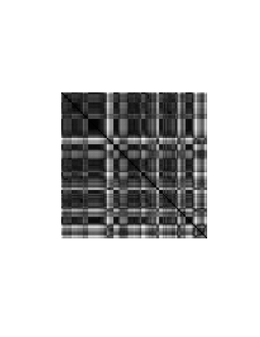
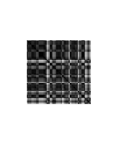
Figure 3. (Left) Distance matrix obtained from computing the best rigid transformation that maps the corresponding labeled landmarks from the teeth dataset described in Section 6.1. (Right) Distance matrix obtained from computing the SDP distance $\tilde{d}_{\mathcal{GH},p}$ with $p=1$. Darker color corresponds to smaller distance. We observe the same distance patterns in both matrices even though the scales are different.

6.1. Classification using the distance $\tilde{d}_{\mathcal{GH}}$

In order to validate our distance numerically we compare with the numerical experiments described in [BLSC⁺11], using data and algorithms available on Yaron Lipman’s personal website [Lip11]. As we describe below, we find that our procedure produces results that are competitive with this procedure.

In [BLSC⁺11] the authors propose an algorithm to automatically quantify the geometric similarity of anatomical surfaces based on a distance inspired by the Gromov-Wasserstein distance which is invariant under conformal maps. They experiment with a real dataset coming from surfaces of teeth of different species; they compare the results of their algorithm with a method based on an expert selecting 16 landmarks on each tooth and then finding the best rigid transformation to match the labeled landmarks. Specifically, they work with a dataset consisting of 116 teeth. For each tooth, they find the closest tooth according to each distance, and then see whether they are in the same category.

We perform the same experiment on 115 of the teeth (since one of them seems to be in a different scale), but without providing our algorithm with the correspondence between the landmarks. To be precise, we consider the metric spaces

$$X_{i}=\{p^{i}_{1},\ldots p^{i}_{16}\},\quad i=1\ldots 115.$$

The points of these metric spaces are the landmarks chosen by the expert, and the metric is given by the euclidean distance between the landmarks. We compare the distance matrix $\tilde{d}_{\mathcal{GH},p}(X_{i},X_{j})$ with the distance obtained by the software from [Lip11] that finds the best rigid transformation that sends the $n$-th point of $X_{i}$ to the $n$-th point of $X_{j}$ for $n=1,\ldots 16$. See Figure 3 for a visual comparison of the distance matrices.

When running the nearest-neighbor classification test as described above, we obtain very similar performance: $0.85$ frequency of success in our distance against $0.91$ for the conformal Wasserstein distance proposed in [BLSC⁺11] and $0.92$ for the landmark comparison algorithm that uses the a priori known correspondence. We find this result very encouraging given that our algorithm does not make any geometric assumptions about the teeth (e.g., we do not assume they are smooth surfaces), in contrast to [BLSC⁺11].

6.2. Performance of GHMatch

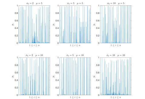
Figure 4. This is the value of convergence of $\mathbf{y}_{k}$ for different parameters $\sigma_{0}$ and $\mu$, for $n=30$. All these $\mathbf{y}$ satisfy the linear constraint $A\mathbf{y}=b$ but the choice of the parameters determine how close the vector $\mathbf{y}$ is to a feasible vector with entries in $\{0,1\}$.

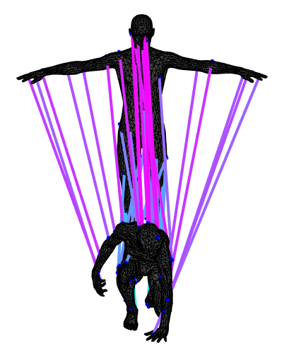
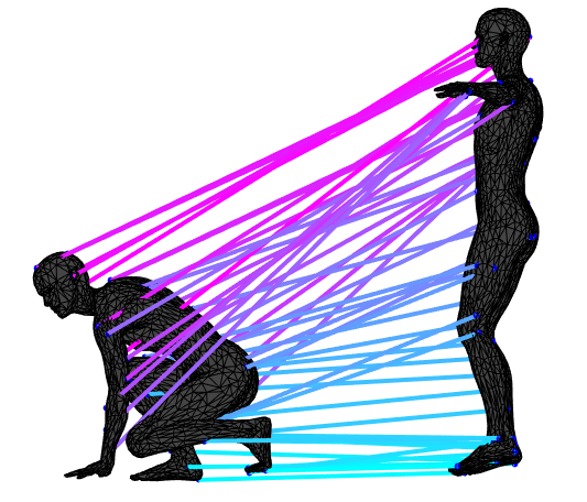
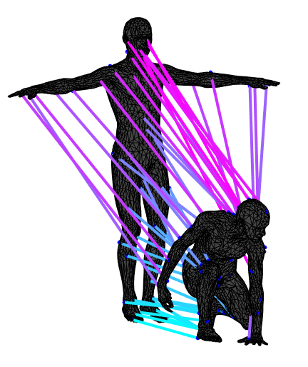
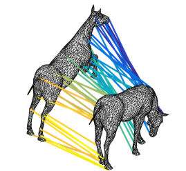
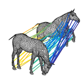
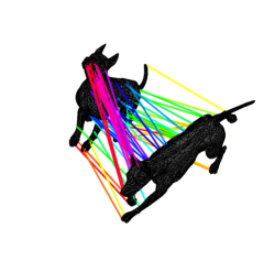
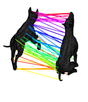
Figure 5. We run GHMatch on 50 points sampled at random from the surfaces, and 60 points for the dogs. The pairwise distances we consider in each figure are the geodesic distances in the mesh. Images that are horizontally aligned correspond to different angles of the same correspondence between the 3D models. Note that for the dogs, the correspondence matches the left legs of one dog with the right legs of the other one (this is a consequence of the symmetry). Also note that there are small imperfections, like the tail of one dog matching with one leg of the other one (this is a consequence of randomly sampling and obtaining different number of points from different dogs tails). The algorithm with 50 sample points runs in less than 6 minutes on a standard 2013 MacBook Air.

In order to evaluate our non-convex optimization formulation of the registration problem, we consider the 3D models from [BBK08] and we sample random points from each model. We run the rank 1 augmented lagrangian optimization from Algorithm 1, using Matlab’s implementation of the reflective trust region algorithm to run the step

$$\mathbf{y}\leftarrow\arg\min_{0\leq\mathbf{y}\leq 1}\mathcal{L}(\mathbf{y},\lambda_{k},\sigma_{k}).$$

In Figure 5 we depict the resulting map between corresponding figures.

By design we know $\sigma_{k}\to\infty$ as $k$ increases, which guarantees that $\|A\mathbf{y}_{k}-b\|\to 0$. However, there is no theoretical guarantee that $\mathbf{y}_{k}$ will converge to a sparse vector with entries in $\{0,1\}$. However, we have observed in our numerical simulations that $\mathbf{y}_{k}$ converges to a fairly sparse vector where most of the entries are close to $0$ or $1$ provided a good choice of the parameters $\mu$ and $\sigma_{0}$ (see Figure 4). Moreover, regardless of the choice of the parameters, we find that our thresholding step in the algorithm often obtains a map that is bijective.

Remark 6.1.

As an alternative to the selection of parameters $\sigma_{0}$ and $\lambda$, a thresholding step could be introduced inside the main iteration (lines 5 to 9) to enforce sparsity of the resulting $\mathbf{y}$.

References

- [Ban15] Afonso S Bandeira. A note on probably certifiably correct algorithms. Comptes Rendus Mathematique, to appear, 2015.
- [BBI01] Dmitri Burago, Yuri Burago, and Sergei Ivanov. A course in metric geometry, volume 33. American Mathematical Society Providence, 2001.
- [BBK08] Alexander Bronstein, Michael Bronstein, and Ron Kimmel. Numerical Geometry of Non-Rigid Shapes. Springer Publishing Company, Incorporated, 1 edition, 2008.
- [BLSC+11] Doug M. Boyer, Yaron Lipman, Elizabeth St. Clair, Jesus Puente, Biren A. Patel, Thomas Funkhouser, Jukka Jernvall, and Ingrid Daubechies. Algorithms to automatically quantify the geometric similarity of anatomical surfaces. Proceedings of the National Academy of Sciences, 108(45):18221–18226, 2011.
- [CK14] Connor Clark and Jugal Kalita. A comparison of algorithms for the pairwise alignment of biological networks. Bioinformatics, 2014.
- [DL16] Nadav Dym and Yaron Lipman. Exact recovery with symmetries for procrustes matching. arXiv preprint arXiv:1606.01548, 2016.
- [Ele12] Gábor Elek. Samplings and observables. limits of metric measure spaces. arXiv:1205.6936, 2012.
- [Gro81] Mikhail Gromov. Groups of polynomial growth and expanding maps. Inst. Hautes Études Sci. Publ. Math., (53):53–73, 1981.
- [Gro01] Mikhail Gromov. Metric Structures for Riemannian and Non-Riemannian Spaces. Progress in Mathematics. Birkhäuser, 2001.
- [IMPV15] Takayuki Iguchi, Dustin G. Mixon, Jesse Peterson, and Soledad Villar. Probably certifiably correct k-means clustering. arXiv:1509.07983, 2015.
- [KKBL15] Itay Kezurer, Shahar Z. Kovalsky, Ronen Basri, and Yaron Lipman. Tight relaxation of quadratic matching. Computer Graphics Forum, 34(5):115–128, 2015.
- [Lip11] Yaron Lipman. Software and teeth dataset, 2011.
- [LV09] John Lott and Cédric Villani. Ricci curvature for metric-measure spaces via optimal transport. Ann. of Math. (2), 169(3):903–991, 2009.
- [MDK+16] Haggai Maron, Nadav Dym, Itay Kezurer, Shahar Kovalsky, and Yaron Lipman. Point registration via efficient convex relaxation. ACM Trans. Graph., 35(4):73:1–73:12, July 2016.
- [Mém07] Facundo Mémoli. On the use of Gromov-Hausdorff Distances for Shape Comparison. pages 81–90, Prague, Czech Republic, 2007. Eurographics Association.
- [Mém11] Facundo Mémoli. Gromov-Wasserstein distances and the metric approach to object matching. Foundations of Computational Mathematics, pages 1–71, 2011. 10.1007/s10208-011-9093-5.
- [MS05] Facundo Mémoli and Guillermo Sapiro. A theoretical and computational framework for isometry invariant recognition of point cloud data. Found. Comput. Math., 5(3):313–347, 2005.
- [NW06] Jorge Nocedal and Stephen J. Wright. Numerical Optimization. Springer, New York, 2nd edition, 2006.
- [OWWZ14] Ryan O’Donnell, John Wright, Chenggang Wu, and Yuan Zhou. Hardness of robust graph isomorphism, lasserre gaps, and asymmetry of random graphs. In Proceedings of the Twenty-Fifth Annual ACM-SIAM Symposium on Discrete Algorithms, pages 1659–1677. SIAM, 2014.
- [PCS16] Gabriel Peyré, Marco Cuturi, and Justin Solomon. Gromov-wasserstein averaging of kernel and distance matrices. In Proc. ICML’16, pages 2664–2672, 2016.
- [Stu06] Karl-Theodor Sturm. On the geometry of metric measure spaces. I. Acta Math., 196(1):65–131, 2006.
- [Vil03] Cédric Villani. Topics in optimal transportation. Graduate studies in mathematics. American Mathematical Society, cop., Providence (R.I.), 2003.
- [YST15] Liuqin Yang, Defeng Sun, and Kim-Chuan Toh. Sdpnal+: a majorized semismooth newton-cg augmented lagrangian method for semidefinite programming with nonnegative constraints. Mathematical Programming Computation, 7(3):331–366, 2015.