An automatically generated code for relativistic inhomogeneous cosmologies

Abstract

The applications of numerical relativity to cosmology are on the rise, contributing insight into such cosmological problems as structure formation, primordial phase transitions, gravitational-wave generation, and inflation. In this paper, I present the infrastructure for the computation of inhomogeneous dust cosmologies which was used recently to measure the effect of nonlinear inhomogeneity on the cosmic expansion rate. I illustrate the code’s architecture, provide evidence for its correctness in a number of familiar cosmological settings, and evaluate its parallel performance for grids of up to several billion points. The code, which is available as free software, is based on the Einstein Toolkit infrastructure, and in particular leverages the automated-code-generation capabilities provided by its component Kranc.

I Introduction

One of the most remarkable successes of general relativity is that it enables the relatively straightforward construction of cosmological models in outstanding agreement with the observational data. As as result, over the past few decades, a remarkably articulate picture of the large-scale Universe has emerged, which combines exact models, relativistic perturbation theory and Newtonian $N$-body simulations into a powerful prediction tool. This is usually referred to as the Concordance Model Ellis et al. (2012).

Over the same period, however, cosmological observations have improved in volume and accuracy, challenging the validity of the previous approach and encouraging researchers to explore fully relativistic, non-perturbative modelling schemes. The imminent perspective of percent-accuracy datasets raises the question of whether the non-linear relativistic effects neglected by the Concordance Model will soon be observable Bull et al. (2016); Debono and Smoot (2016), and perhaps even serve as a testbed for modified-gravity theories Fleury (2016).

The new schemes include relativistic corrections to $N$-body simulations Bruni et al. (2014); Thomas et al. (2015); Adamek et al. (2016a, b, c, 2014, 2015), spherically-symmetric structure-formation studies using a scalar field coupled to Einstein’s equation Torres et al. (2014); Alcubierre et al. (2015); Rekier et al. (2016, 2015), and fully 3D models of inhomogeneous relativistic dust Giblin et al. (2016a); Mertens et al. (2016); Bentivegna and Bruni (2016); Giblin et al. (2016b).

In this work, I describe in detail the approach used in Bentivegna and Bruni (2016), including the system of equations that govern the gravitational and matter fields, the algorithms used to solve them, and the techniques used to implement such algorithms. I will then prove that this scheme reproduces known cosmological solutions filled with a pressureless fluid, such as expanding homogeneous and isotropic spaces, collapsing spherically-symmetric overdensities, and expanding axisymmetric underdensities in the presence of a cosmological constant. This implementation is available as free software to interested researchers .

In the next section, I will illustrate the perfect-fluid representation of cosmic matter fields which underpins the treatment in Bentivegna and Bruni (2016). In section III, I will describe the software modules used to implement such representation, while section IV presents the application of this infrastructure to the computation of various well-known exact cosmologies. In section V I discuss its performance, and conclude in section VI. All quantities are expressed in geometric units, $G=c=1$. Latin letters from the beginning of the alphabet ($a,b,c,\dots$) denote abstract indices, while those from the middle ($i,j,k,\dots$) are used for spatial components.

II Perfect fluids in cosmology

According to general relativity, the Universe’s gravitational field obeys Einstein’s equation coupled to energy and momentum sources such as massive particles or photons. At late times and in rough terms, this results in a homogeneous and isotropic expansion at large scales (say, above one Gigaparsec), with the formation of gravitational structures on smaller scales.

In order to model these processes exactly, one would need to integrate Einstein’s equation on a space without symmetries, with features at several different scales, and with no recourse to the superposition principle as the dynamics is in principle non-linear. Even with the aid of supercomputers, simulating a realistic relativistic Universe is for the moment beyond our reach.

Given the impossibility of a brute-force approach, several simplifications are in order. First of all, one can construct cosmological models where individual particles are represented in statistical terms, via a macroscopic fluid (typically with zero pressure) which fills the Universe. This is already a huge shortcut, which allows us to replace many microscopical degrees of freedom with a few macroscopical, averaged properties such as the density and its first few moments. The process of averaging the microscopical degrees of freedom is of course still nontrivial Ellis et al. (2012); Andersson and Comer (2007), but assuming we can formulate a reasonable continuum-fluid description of matter, the complexity of the problem is greatly reduced.

We now face the problem of integrating the equations of motion for the gravitational field and the hydrodynamical properties of an averaged fluid, the proxy for our cosmic distribution of matter. These equations are just as nonlinear are those we started with, so that numerical integration is the only viable option.

Notice that further simplifications could apply to specific regimes. As an example, since gravitational structures and the associated non-linearities grow with time, there is a period in our cosmic history where the degree of inhomogeneity is so small that perturbations can be described at linear order, where they can be superimposed directly and, by construction, their behaviour is decoupled from that of the underlying spacetime. Such a condition is, for instance, well satisfied at the recombination era, where the Universe is filled with a mix of fluids which is homogeneous and isotropic for a part in $10^{6}$, as testified by the temperature fluctuations in the cosmic-microwave-background photons, a snapshot of the cosmic conditions at that era. As the Universe evolves, however, the relative importance of non-linear mode coupling in the density of the averaged fluid increases.

In general, the numerical integration of the full system of partial differential equations describing matter and gravity is the only viable option. This approach has been pioneered in the study of compact stars Font (2008). In cosmology, matter would typically be modelled as a perfect fluid, characterized by the stress-energy tensor:

$$T_{ab}=\rho hu_{a}u_{b}+pg_{ab}$$ (1)

where $\rho$, $h=1+\epsilon+p/\rho$, $\epsilon$, $p$, and $u_{a}$ are the fluid rest-mass density, specific enthalpy, specific internal energy, pressure, and four-velocity, respectively. The metric tensor is represented by $g_{ab}$.

Introducing a 3+1 decomposition of this quantity, so that the four-dimensional line element reads:

$$ds^{2}=-\alpha^{2}dt^{2}+\gamma_{ij}(\beta^{i}dt+dx^{i})(\beta^{j}dt+dx^{j})$$ (2)

the conservation properties of the fluid can be translated into time evolution equations. Specifically, if the fluid is to satisfy the conservation law

$$\nabla_{a}T^{ab}=0$$ (3)

along with the conservation of the baryon number

$$\nabla_{a}(\rho u^{a})=0$$ (4)

then the following system of equations must hold Font (2008); Anninos (1998):

$$\partial_{t}D = -\partial_{i}(DV^{i})$$ (5)

$$\partial_{t}E = -\partial_{i}(EV^{i})-p\,\partial_{t}W-p\,\partial_{i}(WV^{i})$$ (6)

$$\partial_{t}S_{i} = -\partial_{j}(S_{i}V^{j})+\frac{S_{0}}{2}\partial_{i}g_{00}+S^{j}\partial_{i}\beta_{j}$$ (7)

$$+\frac{S^{j}S^{k}}{2S_{0}}\partial_{i}g_{jk}-\sqrt{-g}\partial_{i}p$$

where I have introduced the variables:

$$D = \rho W$$ (8)

$$E = \rho\epsilon W$$ (9)

$$S_{a} = \rho hu_{a}W$$ (10)

$$V^{i} = \frac{u^{i}}{u^{0}}$$ (11)

$$W = \sqrt{-g}u^{0}$$ (12)

Notice that this system does not include an equation for the pressure. In order to close it, one has to supply an equation of state $p\equiv p(\rho,\epsilon)$. The option $p(\rho,\epsilon)=0$ corresponds to a pressureless fluid, often referred to as dust in cosmological contexts.

In Bentivegna and Bruni (2016), this system was complemented with Einstein’s equation in the Baumgarte-Shapiro-Shibata-Nakamura (BSSN) formulation Shibata and Nakamura (1995); Nakamura et al. (1987); Baumgarte and Shapiro (1998):

$$(\partial_{t}-\beta^{l}\partial_{l})\psi = -\frac{1}{3}\alpha K+\frac{1}{3}\partial_{i}\beta^{i}$$ (13)

$$(\partial_{t}-\beta^{l}\partial_{l})K = -D_{i}D^{i}\alpha+\alpha(\bar{A}_{ij}\bar{A}^{ij}+\frac{1}{3}K^{2})$$ (14)

$$(\partial_{t}-\beta^{l}\partial_{l})\bar{\gamma}_{ij} = -2\alpha\bar{A}_{ij}+2\bar{\gamma}_{i(j}\partial_{k)}\beta^{i}-\frac{2}{3}\bar{\gamma}_{ij}\partial_{k}\beta^{k}$$ (15)

$$(\partial_{t}-\beta^{l}\partial_{l})\bar{A}_{ij} = \psi^{2}(-D_{i}D_{j}\alpha+aR_{ij})^{TF}$$

$$+\alpha(K\bar{A}_{ij}-2\bar{A}_{ik}\bar{A}^{k}_{j})$$

$$+2\bar{A}_{k(i}\partial_{j)}\beta^{k}-\frac{2}{3}A_{ij}\partial_{k}\beta^{k}$$

$$(\partial_{t}-\beta^{l}\partial_{l})\bar{\Gamma}^{i} = \bar{\gamma}^{jk}\beta^{i}\partial_{j}\beta_{k}+\frac{1}{3}\bar{\gamma}^{ij}\partial_{j}\partial_{k}\beta_{k}-\bar{\Gamma}^{j}\partial_{j}\beta^{i}$$

$$+\frac{2}{3}\bar{\Gamma}^{i}\partial_{j}\beta^{j}-2\bar{A}^{ij}\partial_{j}\alpha$$

$$+2\alpha(\bar{\Gamma}^{i}_{jk}\bar{A}^{jk}-3\bar{A}^{jk}\partial_{k}\ln\psi-\frac{2}{3}\bar{\gamma}^{ij}\partial_{j}K)$$

where:

$$\gamma_{ij} = \psi^{-2}\bar{\gamma}_{ij}$$ (18)

$$K_{ij} = \frac{K}{3}\gamma_{ij}+\psi^{-2}\bar{A}_{ij}$$ (19)

$$\bar{\Gamma}^{i} = -\partial_{j}\bar{\gamma}^{ij}$$ (20)

In both the study in Bentivegna and Bruni (2016) and the tests below, the gauge variables $\alpha$ and $\beta^{i}$ are set to one and zero, respectively, at all times.

III Code and setup

Computing the geometry of a spacetime filled with a fluid requires the numerical integration of the equations of relativistic hydrodynamics coupled to Einstein’s equation. The Einstein Toolkit Loffler et al. (2012), an open-source infrastructure for relativistic astrophysics, provides most of the infrastructure necessary for this task: McLachlan mcl ; kra , a module for the integration of Einstein’s equation according to the BSSN formalism (13-II), the AMR package Carpet Schnetter et al. (2004); car , and a software framework called Cactus cac that ties together all the different components, and provides correctness enforcement Bentivegna et al. (2009) and an interface to low-level tasks (such as I/O and parallelization), as well as to user-provided scientific modules. The infrastructure also contains CT_MultiLevel, a multigrid elliptic solver that can be used for the generation of initial data Bentivegna (2014).

In order to carry out the evolution of cosmological models with fluids, one must supply a module that integrates the corresponding equations. Perfect fluids, for instance, are governed by the system (5-7). The Einstein Toolkit provides, via the Kranc package, a mechanism for the generation of code representing the discretization of arbitrary first-order-in-time systems of partial differential equations.

A new module, called CT_Dust and presented in this paper, is constructed using this mechanism. Specifically, the module implements the following recipe:

• It computes initial conditions for the hydrodynamic variables $\rho$, $\epsilon$, $p$ and $u^{a}$, and fills the stress-energy tensor with these values;

• It converts the primitive variables $\rho$, $\epsilon$, and $u^{a}$ into $D$, $E$, and $S^{a}$ using equations (8-10);

• It provides a fourth-order-in-space discretization of the system (5-7), and uses it to update $D$, $E$, and $S^{a}$;

• It converts these variables back into the primitive ones, and fills the stress-energy tensor with the updated values required for the integration of Einstein’s equation.

The various operations entailed by this recipes, such as the expansion of tensorial expressions, the discretization of derivatives, and the optional coordinate transformations, are turned into C++ code automatically by Kranc, a fast and reliable route to the implementation of complex equations and initial conditions. In order to illustrate the advantages of automated code generation in this context, I list some of the full expressions involved in the example of section IV.2 (a collapsing, spherically-symmetric model) in Appendix A.

Two important facts are worth mentioning: first, recovering the primitive variables usually involves a root-finding algorithm, as the relationships (8-10) cannot be inverted analytically. This step is almost trivially implemented in CT_Dust as Kranc provides an interface to corresponding tools in Mathematica. Second, relativistic astrophysics applications almost invariably require the deployment of shock-capturing discretization schemes to correctly resolve and evolve fluid discontinuities. This procedure is necessary, for instance, in scenarios where the fluid is concentrated in compact regions surrounded by vacuum, as would be the case for a neutron star. In the cosmological applications described in Bentivegna and Bruni (2016), however, this is hardly relevant. For this reason, at this stage CT_Dust only employs standard centered finite-differencing.

IV Code tests

In this section, I verify that the scheme described in section III and implemented in CT_Dust is able to reproduce three well-known cosmological models: the flat Friedman-Lemaître-Robertson-Walker (FLRW) spacetime, a Lemaître-Tolman-Bondi (LTB) spherical collapse model, and an axisymmetric Szekeres model with a positive cosmological constant. In the Ellis & van Elst classification of Ellis and van Elst (1998), these models belong to the $(s=3,q=3)$, $(s=2,q=1)$, and $(s=1,q=1)$ classes, respectively.

IV.1 A FLRW model

The simplest application of the hydrodynamical equations illustrated above is obtained by coupling this system to Einstein’s equation and evolving maximally-symmetric initial data, i.e. 3D spaces of constant scalar curvature. In cosmology, these spaces and their time development are referred to as FLRW models, and depending on the equation of state their time behavior can be integrated exactly or through the solution of an ordinary differential equation. They are therefore ideal for a code test.

The case where the spatial curvature is null and the equation of state is given by $p=0$ is called the Einstein-de Sitter (EdS) solution. I integrate the coupled system on a domain given by $-L\leq\{x,y,z\}\leq L$, with periodic boundary conditions at the faces and resolution $\Delta_{x}=\Delta_{y}=\Delta_{z}=0.1L\equiv\Delta$. For initial data, I choose:

$$t_{\rm ini} = \frac{2}{3H_{\rm ini}}$$ (21)

$$\gamma^{\rm ini}_{ij} \equiv \gamma_{ij}(t_{\rm ini})=\delta_{ij}$$ (22)

$$\rho_{\rm ini} \equiv \rho(t_{\rm ini})=\frac{3H_{\rm ini}^{2}}{8\pi}$$ (23)

where I have expressed all dimensional quantities in terms of the initial expansion rate $H_{\rm ini}$. The volume element and density of the EdS model subsequently vary in time as:

$$\sqrt{\gamma/\gamma^{\rm ini}}=\left(t/t_{\rm ini}\right)^{2}=\rho_{\rm ini}/\rho$$ (24)

where $\gamma$ is the determinant of $\gamma_{ij}$. Setting $H_{\rm ini}=\frac{2}{3L}$, in particular, the initial data takes the form:

$$t_{\rm ini} = L$$ (25)

$$\gamma_{\rm ini} = 1$$ (26)

$$\rho_{\rm ini} = \frac{1}{6\pi L^{2}}$$ (27)

Normalizing these quantities with respect to a different value of $H_{\rm ini}$ or expressing them in physical units is trivial.

I evolve this initial data using $\Delta t=0.2\Delta$ up to $t=1000L$, and plot the truncation error for $a(t)\equiv\gamma(t)^{1/6}$, $H(t)\equiv\dot{a}(t)/a(t)$, and $\rho(t)$ in Figure 1. I run an additional resolution $\Delta/2$, also plotted in Figure 1. One observes, as expected, that the numerical estimates for all plotted quantities converge to the exact solution at fourth order in the limit $\Delta\to 0$. As a measure of the accumulated numerical error in this timespan, I also examine how well the mass $\sqrt{\gamma}\rho$ of the cubic cell is conserved throughout the evolution. As can be seen in Figure 1, this quantity is conserved down to the roundoff level. Finally, two plots of the Hamiltonian-constraint violation (unscaled and scaled by the density) are shown, which again demonstrate fourth-order convergence to the exact solution.

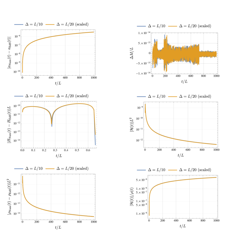
Figure 1: Left column: truncation errors in the volume element, expansion rate and density of the EdS solution, for two different resolutions $\Delta=L/10$ and $L/20$ (the latter rescaled by the expected factor for fourth-order convergence). Right column: violations in the total-mass conservation and the Hamiltonian constraint (absolute and normalized to the density), also for two resolutions.

IV.2 A LTB model

Another relevant class of cosmologies is given by the spherically-symmetric LTB models, represented by the line element Ellis and van Elst (1998):

$$ds^{2}=-dt^{2}+X^{2}(t,r)dr^{2}+Y^{2}(t,r)d\Omega^{2}$$ (28)

The corresponding metric tensor is a solution of Einstein’s equation if:

$$X(t,r) = \pm\frac{|Y^{\prime}(t,r)|}{1+2E(r)}$$ (29)

$$Y(t,r) = \frac{M(r)}{\epsilon(r)}\Phi_{0}(t,r)$$ (30)

$$\rho(t,r) = \frac{M^{\prime}(r)}{4\pi Y^{2}(t,r)Y^{\prime}(t,r)}$$ (31)

where $E(r)$ and $M(r)$ are freely specifiable radial functions, the prime denotes differentiation with respect to $r$, and:

$$\epsilon(r) = \left\{\begin{array}[]{rr}2E(r)&\qquad\textrm{for }E(r)>0\\ 1&\textrm{for }E(r)=0\\ -2E(r)&\textrm{for }E(r)<0\end{array}\right.$$ (35)

$$\Phi_{0}(t,r) = \left\{\begin{array}[]{ll}\cosh(\eta(t,r))-1&\textrm{for }E(r)>0\\ \eta^{2}(t,r)/2&\textrm{for }E(r)=0\\ 1-\cos(\eta(t,r))&\textrm{for }E(r)<0\end{array}\right.$$ (39)

The function $\eta(t,r)$ is a solution of the equation

$$\frac{|\epsilon(r)|^{3/2}(t-t_{\rm B}(r))}{M(r)}=\xi(\eta(t,r))$$ (40)

where:

$$\xi(\eta)=\left\{\begin{array}[]{ll}\sinh\eta-\eta&\qquad\textrm{for }E(r)>0\\ \eta^{3}/6&\qquad\textrm{for }E(r)=0\\ \eta-\sin\eta&\qquad\textrm{for }E(r)<0\end{array}\right.$$ (41)

This general form can describe models with constant-time spaces of any curvature, depending on the value of $E(r)$. Notice that the metric tensor is degenerate on the curves $(r,t_{B}(r))$; like $E(r)$ and $M(r)$, the function $t_{B}(r)$ can also be chosen arbitrarily, allowing one to construct models with space-dependent Big Bangs or Big Crunches.

Here, I choose a so-called “parabolic” (i.e., $E(r)=0$) model where:

$$t_{B}(r)=\tilde{t}-\frac{1}{1+(r/\tilde{r})^{2}}$$ (42)

and the mass function profile is set to the EdS value:

$$M(r)=\frac{2}{9}r^{3}$$ (43)

The corresponding expressions for the metric tensor and the matter density in both polar and cartesian coordinates can be found in Appendix A.

Much like in the previous section, there is an overall length scale $L$ which can be set freely. I use the above expressions to set the initial conditions at $t=L$ in the box $-L\leq\{x,y,z\}\leq L$, with spatial resolutions $\Delta=L/40$ and $\Delta/2$ and boundary conditions set to the analytic solution. I also use $\tilde{t}=5L$ and $\tilde{r}=\sqrt{1/10}L$.

With the chosen parameters, the model will incur a curvature singularity at the origin at $t=4L$; correspondingly, I observe that the density grows unbounded and the volume element shrinks to zero at this point. The evolution is otherwise well behaved and close to the analytical model, to which it converges to fourth order. I illustrate the spatial profiles of the density, the metric component $g_{xx}$, and the extrinsic curvature component $K_{xx}$ along the $z$ axis in the first column of Figure 2. In the second column, the convergence of some of the fields at the representative point $P=(1/2,1/2,1/2)$ as a function of time is shown.

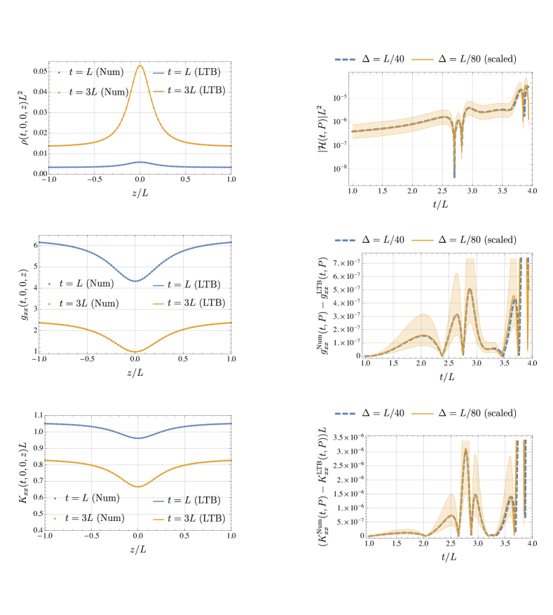
Figure 2: Spatial profiles and temporal evolution for a collapsing LTB model. Left column: spatial profiles for $\rho$, $g_{xx}$, and $K_{xx}$ on the $z$ axis initially ($t=L$) and at $t=3L$. Right column: convergence plot for the Hamiltonian constraint violation $\cal{H}$, $g_{xx}$, and $K_{xx}$ as a function of time at a point $P=(1/2,1/2,1/2)$. The blue dashed line represents the truncation error for the coarser resolution $\Delta=L/40$, while the thicker yellow line is the truncation error for the finer resolution $\Delta=L/80$, rescaled for fourth-order convergence. The thinner yellow lines represent the scaling expected for third- and fifth-order convergence.

IV.3 A Szekeres model

One can further release the symmetry assumptions by considering models invariant under the action of a one-dimensional isotropic group Ellis and van Elst (1998), such as the Szekeres class of models analyzed by Meures & Bruni in Meures and Bruni (2011).

In this spacetime, the density can be made axisymmetric (say, around the $z$-axis) with an arbitrary profile along $z$. The line element can be written as:

$$ds^{2}=-dt^{2}+S(t)^{2}\left[dx^{2}+dy^{2}+Z(t,z)^{2}dz^{2}\right]$$ (44)

where

$$S(t)=\left(\frac{1-\Omega_{\Lambda}}{\Omega_{\Lambda}}\right)^{1/3}\sinh^{2/3}\left[\frac{3}{2}H_{\rm ini}\sqrt{\Omega_{\Lambda}}(t+t_{\star})\right]$$ (45)

$$Z(t,z)=1+(1-\sin kz)[f_{+}(t+t_{\star})+B(x^{2}+y^{2})]$$ (46)

Here, $\Lambda$ and $\Omega_{\Lambda}$ are the cosmological constant and its associated density parameter, $k$ is an arbitrary wave number, $B$ is given by:

$$B=\frac{3}{4}H_{\rm ini}^{2}\left[\Omega_{\Lambda}(1-\Omega_{\Lambda})^{2}\right]^{1/3}$$ (47)

and $f_{+}(t)$ is a solution of:

$$f^{\prime\prime}+\frac{4}{3}\coth\left(\sqrt{\frac{3\Lambda}{4}}t\right)f^{\prime}-\frac{2}{3}\frac{1}{\sinh^{2}\left(\sqrt{\frac{3\Lambda}{4}}t\right)}f=0$$ (48)

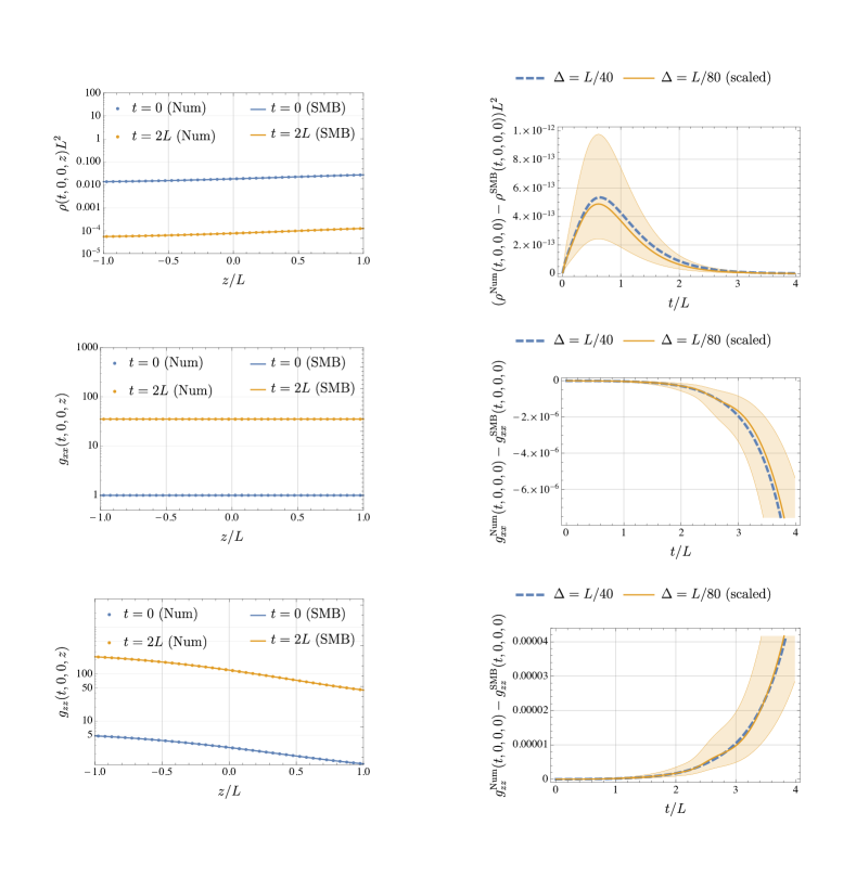
Figure 3: Left column: density and metric components $g_{xx}$ and $g_{zz}$ along the $z$-axis at $t=0$ and $t=2L$, for a grid spacing $\Delta=L/40$. Right column: truncation errors for the above quantities and two resolutions $\Delta=L/40$ and $L/80$. The blue dashed line represents the truncation error for the coarser resolution, while the thicker yellow line is the truncation error for the finer resolution, rescaled for fourth-order convergence. The thinner yellow lines represent the scaling expected for third- and fifth-order convergence.

I set initial conditions for this model in a domain $-L\leq{x,y,z}\leq L$ on the hypersurface at $t=0$, with $\Lambda=2.25L^{2}$ (so that $\Omega_{\Lambda}=0.75$), $H_{\rm ini}=L^{-1}$, $k=\pi$, $t_{\star}=2\sinh^{-1}(\sqrt{\Omega_{\Lambda}/(1-\Omega_{\Lambda})})/(3H_{\rm ini}\sqrt{\Omega_{\Lambda}})$; this is then evolved in time, applying boundary conditions from the exact solution at all times. Figure 3 illustrates the spatial profile and the convergence results for this model. Again, the results exhibit fourth-order convergence to the exact solution.

V Performance and scaling

Even the highest-resolution simulations described in section IV can be run on a laptop with a moderate amount of RAM. Table 1 shows a typical throughput for runs in this range.

Table 1: Run performance on a 2.9GHz Intel Core i5 laptop with 16GB of RAM.

Number of	Memory	Run speed
points $N$	(GB)	($L$/hour)
$47^{3}$	0.19	28
$87^{3}$	1.2	2.1
$167^{3}$	8.7	0.15

As shown in Figure 4, the memory required by each simulation and the execution speed roughly scale as $N$ and $N^{-4/3}$ respectively, as expected.

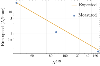
Figure 4: Run speed for grid sizes with $N=46^{3},86^{3},166^{3}$, normalized to the speed at $N=46^{3}$. The reference curve is given by $N^{-4/3}$.

Thanks to its parallel capabilities, the code can also leverage a much higher number of processors, allowing for larger grid sizes. The weak- and strong-scaling properties for grids of up to several billion points are shown in tables 2-3 and Figures 5-6, for runs carried out on the Marconi system at CINECA. The data shows that, keeping the number of points per processing core constant, the problem size can be scaled up to $1447^{3}$ points, with a degradation in run speed of at most $8.1\%$. Furthermore, the solution of a fixed-size problem can be accelerated by a factor of $28$, with a parallel efficiency which is never below $76\%$. It is worth noting that the range of these tests was solely limited by the maximum job size allowed on Marconi.

Table 2: Weak scaling test on CINECA’s Marconi supercomputer. Each node contains 36 processing cores.

Number of	Memory	Number of	Run speed
points $N$	(TB)	nodes $n$	($L$/ hour)
$647^{3}$	0.54	6	0.037
$807^{3}$	1.1	15	0.036
$967^{3}$	1.8	30	0.037
$1127^{3}$	2.9	56	0.035
$1287^{3}$	4.3	94	0.034
$1447^{3}$	8.7	151	0.034

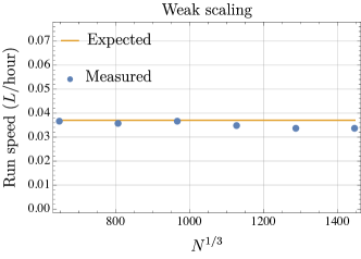
Figure 5: Weak scaling test for the simulations in Table 2.

Table 3: Strong scaling test on CINECA’s Marconi supercomputer. Each node contains 36 processing cores.

Number of	Number of	Run speed
points $N$	nodes $n$	($L$/hour)
$647^{3}$	6	0.037
$647^{3}$	9	0.054
$647^{3}$	12	0.068
$647^{3}$	15	0.085
$647^{3}$	30	0.17
$647^{3}$	100	0.50
$647^{3}$	166	0.78

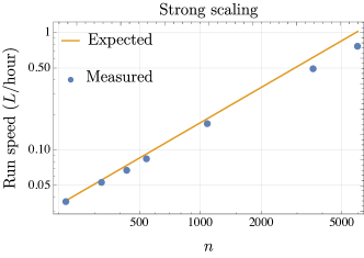
Figure 6: Strong scaling test for the simulations in Table 3. The slope of the reference curve is one.

VI Conclusions

I have described a free-software infrastructure for the computation of inhomogeneous cosmologies through the integration of Einstein’s equation coupled to the equations of relativistic hydrodynamics. The first physical results obtained by this infrastructure have appeared in Bentivegna and Bruni (2016). This companion paper details the algorithms that form the code, provides verification of its behavior in known scenarios, and outlines its computational performance.

As illustrated in Bentivegna and Bruni (2016); Giblin et al. (2016a, b); Mertens et al. (2016), the ability to model the relativistic effects at play in the large-scale Universe opens the road to a better comprehension of its evolution, content, and appearance. The physics of this system is not only one of the core cultural successes of the theory of general relativity, but also a basic ingredient in the study of many other phenomena of astrophysical and cosmological nature. The infrastructure described in this work will surely enable many of the future studies in this direction.

Appendix A The LTB spacetime in Cartesian coordinates

In polar coordinates, the non-zero components of the metric tensor of the LTB model described in section IV.2 take the following form:

$$g_{rr}(t,r) = \frac{\left(3r^{4}(t-\tilde{t})+r^{2}\tilde{r}^{2}(6t-6\tilde{t}-1)+3\tilde{r}^{4}(t-\tilde{t}+1)\right)^{2}}{9\left(r^{2}+\tilde{r}^{2}\right)^{4}\left(-\frac{\tilde{r}^{2}}{r^{2}+\tilde{r}^{2}}-t+\tilde{t}\right)^{2/3}}$$ (49)

$$g_{\theta\theta}(t,r) = r^{2}\left(-\frac{\tilde{r}^{2}}{r^{2}+\tilde{r}^{2}}-t+\tilde{t}\right)^{4/3}$$ (50)

$$g_{\phi\phi}(t,r) = \left(x^{2}+y^{2}\right)\left(-\frac{\tilde{r}^{2}}{r^{2}+\tilde{r}^{2}}-t+\tilde{t}\right)^{4/3}$$ (51)

whilst the density is given by:

$$\rho(t,r)=\frac{\left(r^{2}+\tilde{r}^{2}\right)^{3}}{2\pi\left(r^{2}(t-\tilde{t})+\tilde{r}^{2}(t-\tilde{t}+1)\right)\left(3r^{4}(t-\tilde{t})+r^{2}\tilde{r}^{2}(6t-6\tilde{t}-1)+3\tilde{r}^{4}(t-\tilde{t}+1)\right)}$$ (52)

The same quantities are given, in Cartesian coordinates, by:

$$g_{xx}(t,x,y,z) = r^{-4}\left(r^{2}\left(y^{2}+z^{2}\right)\left(-\frac{\tilde{r}^{2}}{r^{2}+\tilde{r}^{2}}-t+\tilde{t}\right)^{4/3}+\right.$$ (53)

$$\frac{x^{4}\left(3r^{4}(t-\tilde{t})+r^{2}\tilde{r}^{2}(6t-6\tilde{t}-1)+3\tilde{r}^{4}(t-\tilde{t}+1)\right)^{2}}{9\left(r^{2}+\tilde{r}^{2}\right)^{4}\left(-\frac{\tilde{r}^{2}}{r^{2}+\tilde{r}^{2}}-t+\tilde{t}\right)^{2/3}}+$$

$$\left.\frac{x^{2}\left(y^{2}+z^{2}\right)\left(3r^{4}(t-\tilde{t})+r^{2}\tilde{r}^{2}(6t-6\tilde{t}-1)+3\tilde{r}^{4}(t-\tilde{t}+1)\right)^{2}}{9\left(r^{2}+\tilde{r}^{2}\right)^{4}\left(-\frac{\tilde{r}^{2}}{r^{2}+\tilde{r}^{2}}-t+\tilde{t}\right)^{2/3}}\right)$$

$$g_{xy}(t,x,y,z) = -\frac{8\tilde{r}^{2}xy\left(3r^{4}(t-\tilde{t})+r^{2}\tilde{r}^{2}(6t-6\tilde{t}+1)+3\tilde{r}^{4}(t-\tilde{t}+1)\right)}{9\left(r^{2}+\tilde{r}^{2}\right)^{4}\left(-\frac{\tilde{r}^{2}}{r^{2}+\tilde{r}^{2}}-t+\tilde{t}\right)^{2/3}}$$ (54)

$$\rho(t,x,y,z) = \frac{\left(r^{2}+\tilde{r}^{2}\right)^{3}}{2\pi\left(r^{2}(t-\tilde{t})+\tilde{r}^{2}(t-\tilde{t}+1)\right)\left(3r^{4}(t-\tilde{t})+r^{2}\tilde{r}^{2}(6t-6\tilde{t}-1)+3\tilde{r}^{4}(t-\tilde{t}+1)\right)}$$ (55)

where $r=\sqrt{x^{2}+y^{2}+z^{2}}$ and, due the spherical symmetry, the other components of the metric can be obtained by permuting the spatial coordinates. The computation of these quantities and their derivatives is greatly simplified by the ability to generate code automatically.

References

- Ellis et al. (2012) G. Ellis, R. Maartens, and M. MacCallum, Relativistic Cosmology (Cambridge University Press, 2012).
- Bull et al. (2016) P. Bull et al., “Beyond CDM: Problems, solutions, and the road ahead,” Phys. Dark Univ. 12, 56–99 (2016).
- Debono and Smoot (2016) I. Debono and G. F. Smoot, “General Relativity and Cosmology: Unsolved Questions and Future Directions,” Universe 2, 23 (2016).
- Fleury (2016) P. Fleury, “Cosmic backreaction and Gauss’s law,” (2016), arXiv:1609.03724 [gr-qc] .
- Bruni et al. (2014) M. Bruni, D. B. Thomas, and D. Wands, “Computing General Relativistic effects from Newtonian N-body simulations: Frame dragging in the post-Friedmann approach,” Phys. Rev. D89, 044010 (2014).
- Thomas et al. (2015) D. B. Thomas, M. Bruni, and D. Wands, “The fully non-linear post-Friedmann frame-dragging vector potential: Magnitude and time evolution from N-body simulations,” Mon. Not. Roy. Astron. Soc. 452, 1727–1742 (2015).
- Adamek et al. (2016a) J. Adamek, D. Daverio, R. Durrer, and M. Kunz, “gevolution: a cosmological N-body code based on General Relativity,” JCAP 1607, 053 (2016a).
- Adamek et al. (2016b) J. Adamek, D. Daverio, R. Durrer, and M. Kunz, “General relativity and cosmic structure formation,” Nature Phys. 12, 346–349 (2016b).
- Adamek et al. (2016c) J. Adamek, M. Gosenca, and S. Hotchkiss, “Spherically Symmetric N-body Simulations with General Relativistic Dynamics,” Phys. Rev. D93, 023526 (2016c).
- Adamek et al. (2014) J. Adamek, R. Durrer, and M. Kunz, “N-body methods for relativistic cosmology,” Class. Quant. Grav. 31, 234006 (2014).
- Adamek et al. (2015) J. Adamek, C. Clarkson, R. Durrer, and M. Kunz, “Does small scale structure significantly affect cosmological dynamics?” Phys. Rev. Lett. 114, 051302 (2015).
- Torres et al. (2014) J. M. Torres, M. Alcubierre, A. Diez-Tejedor, and D. Núñez, “Cosmological nonlinear structure formation in full general relativity,” Phys. Rev. D90, 123002 (2014).
- Alcubierre et al. (2015) M. Alcubierre, A. de la Macorra, A. Diez-Tejedor, and J. M. Torres, “Cosmological scalar field perturbations can grow,” Phys. Rev. D92, 063508 (2015).
- Rekier et al. (2016) J. Rekier, A. Fuzfa, and I. Cordero-Carrion, “Nonlinear cosmological spherical collapse of quintessence,” Phys. Rev. D93, 043533 (2016).
- Rekier et al. (2015) J. Rekier, I. Cordero-Carrión, and A. Füzfa, “Spherically Symmetric solutions on a cosmological dynamical background with BSSN equations,” Proceedings, Spanish Relativity Meeting: Almost 100 years after Einstein Revolution (ERE 2014): Valencia, Spain, September 1-5, 2014, J. Phys. Conf. Ser. 600, 012062 (2015).
- Giblin et al. (2016a) J. T. Giblin, J. B. Mertens, and G. D. Starkman, “Departures from the Friedmann-Lemaitre-Robertston-Walker Cosmological Model in an Inhomogeneous Universe: A Numerical Examination,” Phys. Rev. Lett. 116, 251301 (2016a).
- Mertens et al. (2016) J. B. Mertens, J. T. Giblin, and G. D. Starkman, “Integration of inhomogeneous cosmological spacetimes in the BSSN formalism,” Phys. Rev. D93, 124059 (2016).
- Bentivegna and Bruni (2016) E. Bentivegna and M. Bruni, “Effects of nonlinear inhomogeneity on the cosmic expansion with numerical relativity,” Phys. Rev. Lett. 116, 251302 (2016).
- Giblin et al. (2016b) J. T. Giblin, J. B. Mertens, and G. D. Starkman, “Observable Deviations from Homogeneity in an Inhomogeneous Universe,” (2016b), arXiv:1608.04403 [astro-ph.CO] .
- Note (1) The code is distributed under the GNU General Public License, version 3 or later (GNU GPLv3+) from the repository https://bitbucket.org/eloisa/ctthorns.git.
- Andersson and Comer (2007) N. Andersson and G. L. Comer, “Relativistic fluid dynamics: Physics for many different scales,” Living Rev. Rel. 10, 1 (2007).
- Font (2008) J. A. Font, “Numerical hydrodynamics and magnetohydrodynamics in general relativity,” Living Rev. Rel. 11, 1 (2008).
- Anninos (1998) P. Anninos, “Plane-symmetric cosmology with relativistic hydrodynamics,” Phys. Rev. D 58, 064010 (1998).
- Shibata and Nakamura (1995) M. Shibata and T. Nakamura, “Evolution of three-dimensional gravitational waves: Harmonic slicing case,” Phys. Rev. D 52, 5428–5444 (1995).
- Nakamura et al. (1987) T. Nakamura, K. Oohara, and Y. Kojima, “General relativistic collapse to black holes and gravitational waves from black holes,” Prog. Theor. Phys. Suppl. 90, 1–218 (1987).
- Baumgarte and Shapiro (1998) T. W. Baumgarte and S. L. Shapiro, “On the numerical integration of einstein’s field equations,” Phys. Rev. D 59, 024007 (1998).
- Loffler et al. (2012) F. Loffler, J. Faber, E. Bentivegna, T. Bode, P. Diener, et al., “The Einstein Toolkit: A Community Computational Infrastructure for Relativistic Astrophysics,” Class.Quant.Grav. 29, 115001 (2012).
- (28) McLachlan code, https://www.cct.lsu.edu/~eschnett/McLachlan .
- (29) Kranc code, http://kranccode.org .
- Schnetter et al. (2004) E. Schnetter, S. H. Hawley, and I. Hawke, “Evolutions in 3d numerical relativity using fixed mesh refinement,” Class. Quant. Grav. 21, 1465–1488 (2004).
- (31) Carpet code, https://www.carpetcode.org .
- (32) Cactus code, http://www.cactuscode.org .
- Bentivegna et al. (2009) E. Bentivegna, G. Allen, O. Korobkin, and E. Schnetter, “Ensuring Correctness at the Application Level: A Software Framework Approach,” Proceedings of the 2009 Workshop on Component-Based High-Performance Computing, CBHPC 2009 (2009), arXiv:1101.3161 [cs.SE] .
- Bentivegna (2014) E. Bentivegna, “Solving the Einstein constraints in periodic spaces with a multigrid approach,” Class.Quant.Grav. 31, 035004 (2014).
- Ellis and van Elst (1998) G. F. R. Ellis and H. van Elst, “Cosmological models (cargèse lectures 1998),” (1998), gr-qc/9812046v5 .
- Meures and Bruni (2011) N. Meures and M. Bruni, “Exact non-linear inhomogeneities in CDM cosmology,” Phys. Rev. D83, 123519 (2011).