EUROPEAN ORGANIZATION FOR NUCLEAR RESEARCH (CERN)

CERN-EP-2016-213 LHCb-PAPER-2016-028 23 November 2016

Observation of the decay $B^{0}_{s}\rightarrow\phi\pi^{+}\pi^{-}$ and evidence for $B^{0}\rightarrow\phi\pi^{+}\pi^{-}$

The LHCb collaboration

The first observation of the rare decay $B^{0}_{s}\rightarrow\phi\pi^{+}\pi^{-}$ and evidence for $B^{0}\rightarrow\phi\pi^{+}\pi^{-}$ are reported, using $pp$ collision data recorded by the LHCb detector at centre-of-mass energies $\sqrt{s}=7$ and 8 TeV, corresponding to an integrated luminosity of 3 fb^-1. The branching fractions in the $\pi^{+}\pi^{-}$ invariant mass range $400<m(\pi^{+}\pi^{-})<1600{\mathrm{\,Me\kern-1.00006ptV\!/}c^{2}}$ are $[3.48\pm 0.23\pm 0.17\pm 0.35]\times 10^{-6}$ and $[1.82\pm 0.25\pm 0.41\pm 0.14]\times 10^{-7}$ for $B^{0}_{s}\rightarrow\phi\pi^{+}\pi^{-}$ and $B^{0}\rightarrow\phi\pi^{+}\pi^{-}$ respectively, where the uncertainties are statistical, systematic and from the normalisation mode $B^{0}_{s}\rightarrow\phi\phi$. A combined analysis of the $\pi^{+}\pi^{-}$ mass spectrum and the decay angles of the final-state particles identifies the exclusive decays ${B}^{0}_{s}\rightarrow\phi f_{0}(980)$, $B_{s}^{0}\rightarrow\phi f_{2}(1270)$, and $B^{0}_{s}\rightarrow\phi\rho^{0}$ with branching fractions of $[1.12\pm 0.16^{+0.09}_{-0.08}\pm 0.11]\times 10^{-6}$, $[0.61\pm 0.13^{+0.12}_{-0.05}\pm 0.06]\times 10^{-6}$ and $[2.7\pm 0.7\pm 0.2\pm 0.2]\times 10^{-7}$, respectively.

Published on 11th January 2017 as Phys.Rev.D 95, 026007 (2017)

© CERN on behalf of the LHCb collaboration, licence CC-BY-4.0.

 

1 Introduction

The decays ${{B}^{0}_{s}}\!\rightarrow\phi{{\pi}^{+}}{{\pi}^{-}}$ and ${{B}^{0}}\!\rightarrow\phi{{\pi}^{+}}{{\pi}^{-}}$ have not been observed before. They are examples of decays that are dominated by contributions from flavour changing neutral currents (FCNC), which provide a sensitive probe for the effect of physics beyond the Standard Model because their amplitudes are described by loop (or penguin) diagrams where new particles may enter [1]. A well-known example of this type of decay is ${{B}^{0}_{s}}\!\rightarrow\phi\phi$ which has a branching fraction of $1.9\times 10^{-5}$ [2]. First measurements of the $C\!P$-violating phase $\phi_{s}$ in this mode have recently been made by the LHCb collaboration [3, 4]. The decay ${{B}^{0}_{s}}\!\rightarrow\phi f_{0}(980)$ also proceeds via a gluonic $b\rightarrow s$ penguin transition (see Fig. 1(a)), with an expected branching fraction of approximately $2\times 10^{-6}$, based on the ratio of the ${{B}^{0}_{s}}\rightarrow J/\psi f_{0}(980)$ and ${{B}^{0}_{s}}\rightarrow J/\psi\phi$ decays [2]. When large statistics samples are available, similar time-dependent $C\!P$ violation studies will be possible with ${{B}^{0}_{s}}\!\rightarrow\phi f_{0}(980)$.

The decay ${{B}^{0}_{s}}\rightarrow\phi\rho^{0}$ is of particular interest, because it is an isospin-violating $\Delta I=1$ transition which is mediated by a combination of an electroweak penguin diagram and a suppressed $b\rightarrow u$ transition (see Fig. 1(b)). The predicted branching fraction is $[4.4^{+2.2}_{-0.7}]\times 10^{-7}$, and large $C\!P$-violating asymmetries are not excluded [5].

The corresponding ${{B}^{0}}$ decays are mediated by CKM-suppressed $b\rightarrow d$ penguin diagrams, and are expected to have branching fractions an order of magnitude lower than the ${{B}^{0}_{s}}$ decays. The BaBar experiment has set an upper limit on the branching fraction of the decay ${{B}^{0}}\rightarrow\phi\rho^{0}$ of $3.3\times 10^{-7}$ at $90\%$ confidence level [6].

This paper reports a time-integrated and flavour-untagged search, using a dataset with an integrated luminosity of approximately 3 fb^-1 collected by the LHCb detector in 2011 and 2012 at centre-of-mass energies of $\sqrt{s}=$7 and 8 TeV, respectively. This leads to the first observation of ${{B}^{0}_{s}}\!\rightarrow\phi{{\pi}^{+}}{{\pi}^{-}}$ decays, and evidence for ${{B}^{0}}\!\rightarrow\phi{{\pi}^{+}}{{\pi}^{-}}$ decays, with the $\pi^{+}\pi^{-}$ invariant mass in the range $400<m(\pi^{+}\pi^{-})<1600$${\mathrm{\,Me\kern-1.00006ptV\!/}c^{2}}$. A combined angular and $\pi^{+}\pi^{-}$ mass analysis of the ${{B}^{0}_{s}}\!\rightarrow\phi{{\pi}^{+}}{{\pi}^{-}}$ sample identifies contributions from the exclusive decays ${{B}^{0}_{s}}\!\rightarrow\phi f_{0}(980)$, $B_{s}^{0}\rightarrow\phi f_{2}(1270)$, and ${{B}^{0}_{s}}\!\rightarrow\phi\rho^{0}$. There is also a significant S-wave $\pi^{+}\pi^{-}$ contribution in the high-mass region $1350<m(\pi^{+}\pi^{-})<1600$${\mathrm{\,Me\kern-1.00006ptV\!/}c^{2}}$.

The branching fractions for both the inclusive and exclusive decays are determined with respect to the normalisation mode ${{B}^{0}_{s}}\!\rightarrow\phi\phi$. This mode has a very similar topology and a larger branching fraction, which has been measured by the LHCb collaboration [7] to be $\mathcal{B}({{B}^{0}_{s}}\!\rightarrow\phi\phi)=[1.84\pm 0.05\pm 0.07\pm 0.11\pm 0.12]\times 10^{-5}$, where the uncertainties are respectively statistical, systematic, from the fragmentation function $f_{s}/f_{d}$ giving the ratio of ${{B}^{0}_{s}}$ to ${{B}^{0}}$ production at the LHC, and from the measurement of the branching fraction of ${{B}^{0}}\rightarrow\phi{{K}^{*}}^{0}$ at the $B$ factories [8, 9].

Figure 1: Feynman diagrams for the exclusive decays (a) $B_{s}^{0}\rightarrow\phi f_{0}(980)$ and (b) $B_{s}^{0}\rightarrow\phi\rho^{0}$.

2 Detector and software

The LHCb detector [10, 11] is a single-arm forward spectrometer covering the pseudorapidity range $2<\eta<5$. It is designed for the study of particles containing $b$ or $c$ quarks, which are produced preferentially as pairs at small angles with respect to the beam axis. The detector includes a high-precision tracking system consisting of a silicon-strip vertex detector surrounding the $pp$ interaction region, a large-area silicon-strip tracker located upstream of a dipole magnet with a bending power of about $4{\rm\,Tm}$, and three stations of silicon-strip trackers and straw drift tubes placed downstream of the magnet. The tracking system provides a measurement of charged particle momenta with a relative uncertainty that varies from 0.5% at 5${\mathrm{\,Ge\kern-1.00006ptV\!/}c}$ to 1.0% at 200${\mathrm{\,Ge\kern-1.00006ptV\!/}c}$. The minimum distance of a track to a primary $pp$ interaction vertex (PV), the impact parameter (IP), is measured with a resolution of $(15+29/\mbox{$p_{\rm T}$}){\,\upmu\rm m}$, where $p_{\rm T}$ is the component of the momentum transverse to the beam, in ${\mathrm{\,Ge\kern-1.00006ptV\!/}c}$. Different types of charged hadrons are distinguished using information from two ring-imaging Cherenkov detectors. Photon, electron and hadron candidates are identified by a calorimeter system consisting of scintillating-pad and preshower detectors, an electromagnetic calorimeter and a hadronic calorimeter. Muons are identified by a system composed of alternating layers of iron and multiwire proportional chambers.

The trigger [12] consists of a hardware stage, based on information from the calorimeter and muon systems, followed by a software stage, which applies a full event reconstruction. The software trigger requires a two-, three- or four-track secondary vertex with a significant displacement from an associated PV. At least one charged particle must have a transverse momentum $\mbox{$p_{\rm T}$}>1.7{\mathrm{\,Ge\kern-1.00006ptV\!/}c}$ and be inconsistent with originating from the PV. A multivariate algorithm [13] is used for the identification of secondary vertices consistent with the decay of a $b$ hadron into charged hadrons. In addition, an algorithm is used that identifies inclusive $\phi\rightarrow K^{+}K^{-}$ production at a secondary vertex, without requiring a decay consistent with a $b$ hadron.

In the simulation, $pp$ collisions are generated using Pythia 6 [14] with a specific LHCb configuration [15]. Decays of hadronic particles are described by EvtGen [16], in which final-state radiation is generated using Photos [17]. The interaction of the generated particles with the detector and its response are implemented using the Geant4 toolkit [18, *Agostinelli:2002hh] as described in Ref. [20].

3 Selection

The offline selection of candidates consists of two parts. First, a selection with loose criteria is performed that reduces the combinatorial background as well as removing some specific backgrounds from other exclusive ${b}$-hadron decay modes. In a second stage a multivariate method is applied to further reduce the combinatorial background and improve the signal significance.

The selection starts from well-reconstructed particles that traverse the entire spectrometer and have $p_{T}>500{\mathrm{\,Me\kern-1.00006ptV\!/}c}$. Spurious tracks created by the reconstruction are suppressed using a neural network trained to discriminate between these and real particles. A large track IP with respect to any PV is required, consistent with the track coming from a displaced secondary decay vertex. The information provided by the ring-imaging Cherenkov detectors is combined with information from the tracking system to select charged particles consistent with being a kaon, pion or proton. Tracks that are identified as muons are removed at this stage.

Pairs of oppositely charged kaons that originate from a common vertex are combined to form a $\phi$ meson candidate. The transverse momentum of the $\phi$ meson is required to be larger than $0.9{\mathrm{\,Ge\kern-1.00006ptV\!/}c}$ and the invariant mass to be within $10{\mathrm{\,Me\kern-1.00006ptV\!/}c^{2}}$ of the known value [2]. Similarly, pairs of oppositely charged pions are combined if they form a common vertex and if the transverse momentum of the $\pi^{+}\pi^{-}$ system is larger than $1{\mathrm{\,Ge\kern-1.00006ptV\!/}c}$. For this analysis, the invariant mass of the pion pair is required to be in the range $400<m(\pi^{+}\pi^{-})<1600{\mathrm{\,Me\kern-1.00006ptV\!/}c^{2}}$, below the charm threshold. The $\phi$ candidates and $\pi^{+}\pi^{-}$ pairs are combined to form ${{B}^{0}}$ or ${{B}^{0}_{s}}$ meson candidates. To further reject combinatorial background, the reconstructed flight path of the $B$ candidates must be consistent with coming from a PV.

There are several decays of $b$ hadrons proceeding via charmed hadrons that need to be explicitly removed. The decay modes ${{B}^{0}_{s}}\rightarrow{{D}^{-}_{s}}\pi^{+}$ and ${{B}^{0}}\rightarrow{{D}^{-}}\pi^{+}$ are rejected when the invariant mass of the $K^{+}K^{-}\pi^{-}$ system is within 3 standard deviations ($\sigma$) of either $D$ meson mass. The decay mode $\kern 1.79993pt\shortstack{{(\rule[2.15277pt]{12.50002pt}{0.51212pt})} \\ [-.7ex] $\kern-1.79993ptB$}{}\rightarrow\kern 1.79993pt\shortstack{{(\rule[2.15277pt]{12.50002pt}{0.51212pt})} \\ [-.7ex] $\kern-1.79993ptD$}{}K^{\pm}\pi^{\mp}$ is rejected when the invariant mass of either of the $K^{\pm}\pi^{\mp}$ combinations is within 2$\sigma$ of the ${{D}^{0}}$ mass. Backgrounds from $D^{-}$ decays to $K^{+}\pi^{-}\pi^{-}$ and from ${{\mathchar 28931\relax}^{+}_{c}}$ decays to $pK^{-}\pi^{+}$ are removed if the three-body invariant mass, calculated assuming that either a $\pi^{-}$ or a proton has been misidentified as a kaon, is within 3$\sigma$ of the charm hadron mass.

Another background arises from the decay ${{B}^{0}}\rightarrow\phi{{K}^{*}}^{0}$, where the kaon from the decay ${{K}^{*}}^{0}\rightarrow K^{+}\pi^{-}$ is misidentified as a pion. To remove it, the invariant masses $m(K^{+}\pi^{-})$ and $m(K^{+}K^{-}K^{+}\pi^{-})$ are calculated assuming that one of the $K^{+}$ has been misidentified as a $\pi^{+}$, and candidates are rejected if $m(K^{+}\pi^{-})$ is within 3 decay widths of the ${{K}^{*}}^{0}$, and $m(K^{+}K^{-}K^{+}\pi^{-})$ is consistent with the ${{B}^{0}}$ mass to within 3 times the experimental resolution. The higher resonance mode ${{B}^{0}}\rightarrow\phi K_{2}^{*0}(1430)$ is vetoed in a similar fashion. The efficiency of the charm and $\phi{{K}^{*}}^{0}$ vetoes is 94%, evaluated on the ${{B}^{0}_{s}}\!\rightarrow\phi{{\pi}^{+}}{{\pi}^{-}}$ simulation sample, with the $\phi{{K}^{*}}^{0}$ veto being 99% efficient. For the decay ${{B}^{0}}\!\rightarrow\phi{{\pi}^{+}}{{\pi}^{-}}$ this efficiency is reduced to 84% by the larger impact of the $\phi{{K}^{*}}^{0}$ veto.

In the second stage of the selection a boosted decision tree (BDT) [21, 22] is employed to further reduce the combinatorial background. This makes use of twelve variables related to the kinematics of the $B$ meson candidate and its decay products, particle identification for the kaon candidates and the $B$ decay vertex displacement from the PV. It is trained using half of both the simulated signal sample and the background events from the data in the range $5450<m(K^{+}K^{-}\pi^{+}\pi^{-})<5600{\mathrm{\,Me\kern-1.00006ptV\!/}c^{2}}$, and validated using the other half of each sample. For a signal efficiency of 90% the BDT has a background rejection of 99%.

A sample of ${{B}^{0}_{s}}\!\rightarrow\phi\phi$ candidates has been selected using the same methods as for the signal modes, apart from the particle identification criteria and the $m(K^{+}K^{-})$ mass window for the second $\phi$ meson, and without the $\phi K^{*0}$ veto. The BDT deliberately does not include particle identification for the pion candidates, because this part of the selection is different between the signal mode and the ${{B}^{0}_{s}}\!\rightarrow\phi\phi$ normalisation mode.

For the signal mode a tighter selection is made on the pion identification as part of a two-dimensional optimisation together with the BDT output. The figure of merit (FOM) used to maximise the discovery potential for a new signal is[23],

$${\rm FOM}=\frac{\varepsilon_{S}}{5/2+\sqrt{B}}\hskip 2.84544pt,$$

where $\varepsilon_{S}$ is the signal efficiency evaluated using the simulation and $B$ is the number of background candidates expected within a 50${\mathrm{\,Me\kern-1.00006ptV\!/}c^{2}}$ window about the ${B}^{0}_{s}$ mass. The optimised selection on the BDT output and the pion identification has a signal efficiency $\varepsilon_{S}=0.846$.

4 Invariant mass fit

The yields for the inclusive ${{B}^{0}_{s}}\!\rightarrow\phi{{\pi}^{+}}{{\pi}^{-}}$ and ${{B}^{0}}\!\rightarrow\phi{{\pi}^{+}}{{\pi}^{-}}$ signals are determined from a fit to the invariant $K^{+}K^{-}\pi^{+}\pi^{-}$ mass distribution of selected candidates in the range $5100<m(K^{+}K^{-}\pi^{+}\pi^{-})<5600{\mathrm{\,Me\kern-1.00006ptV\!/}c^{2}}$. The fit includes possible signal contributions from both ${{B}^{0}_{s}}$ and ${{B}^{0}}$ decays, as well as combinatorial background. Backgrounds from partially reconstructed decays such as ${{B}^{0}_{s}}\rightarrow\phi\phi(\rightarrow\pi^{+}\pi^{-}\pi^{0})$ and ${{B}^{0}_{s}}\rightarrow\phi\eta^{\prime}(\rightarrow\pi^{+}\pi^{-}\gamma)$ are negligible in the region $m(K^{+}K^{-}\pi^{+}\pi^{-})>5100{\mathrm{\,Me\kern-1.00006ptV\!/}c^{2}}$. After the veto the contribution from ${{B}^{0}}\rightarrow\phi K^{*0}$ can also be neglected.

The line shapes for the ${{B}^{0}_{s}}\!\rightarrow\phi{{\pi}^{+}}{{\pi}^{-}}$ signal and ${{B}^{0}_{s}}\!\rightarrow\phi\phi$ normalisation mode are determined using simulated events, and parameterised by a sum of two Gaussian functions with a common mean and different widths. In the fits to data the means and widths of the narrow Gaussians for the ${{B}^{0}_{s}}$ modes are fitted, but the relative widths and fractions of the broader Gaussians relative to the narrow ones are taken from the simulation. The mean and width of the ${{B}^{0}}$ signal shape are scaled down from ${{B}^{0}_{s}}\!\rightarrow\phi{{\pi}^{+}}{{\pi}^{-}}$ to account for the mass difference [2], and to correct for a slight modification of the ${{B}^{0}}$ shape due to the $\phi{{K}^{*}}^{0}$ veto. The combinatorial background is modelled by an exponential function with a slope that is a free parameter in the fit to the data.

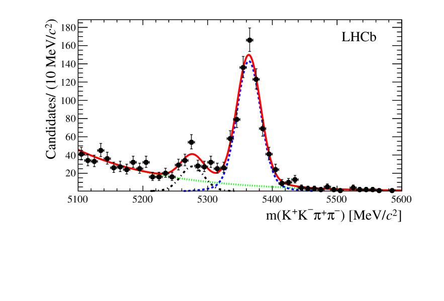
Figure 2: The $K^{+}K^{-}\pi^{+}\pi^{-}$ invariant mass distribution for candidates in the mass range $0.4<m_{\pi\pi}<1.6$${\mathrm{\,Ge\kern-0.90005ptV\!/}c^{2}}$. The fit described in the text is overlaid. The solid (red) line is the total fitted function, the dotted (green) line the combinatorial background, the dashed (blue) line the ${{B}^{0}_{s}}$ and the dot-dashed (black) line the ${{B}^{0}}$ signal component.

Figure 2 shows the result of the extended unbinned maximum likelihood fit to the $m(K^{+}K^{-}\pi^{+}\pi^{-})$ distribution. There is clear evidence for both ${{B}^{0}_{s}}\!\rightarrow\phi{{\pi}^{+}}{{\pi}^{-}}$ and ${{B}^{0}}\!\rightarrow\phi{{\pi}^{+}}{{\pi}^{-}}$ signals. The ${{B}^{0}_{s}}$ and ${{B}^{0}}$ yields are $697\pm 30$ and $131\pm 17$ events, respectively, and the fit has a chi-squared per degree of freedom, $\chi^{2}/\mathrm{ndf}$, of 0.87. Figure 3 shows the $m(K^{+}K^{-}K^{+}K^{-})$ distribution for the ${{B}^{0}_{s}}\!\rightarrow\phi\phi$ normalisation mode, with a fit using a sum of two Gaussians for the ${B}^{0}_{s}$ signal shape. There are $2424\pm 51$ events above a very low combinatorial background. Backgrounds from other decay modes are negligible with this selection.

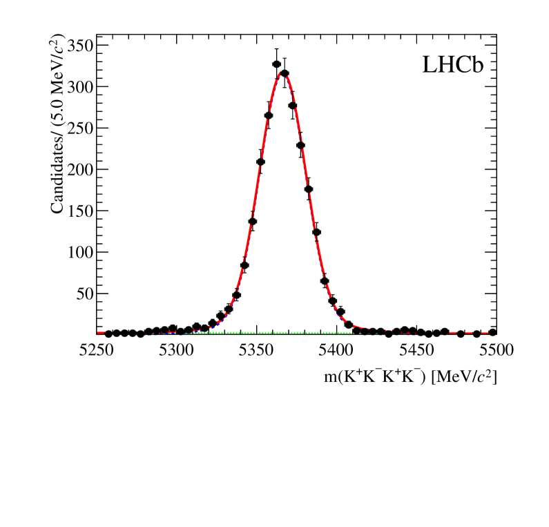
Figure 3: The $K^{+}K^{-}K^{+}K^{-}$ invariant mass distribution after all selection criteria. The solid (red) line is the total fitted function including the ${{B}^{0}_{s}}\!\rightarrow\phi\phi$ signal, and the dashed (green) line is the combinatorial background.

To study the properties of the ${{B}^{0}_{s}}\!\rightarrow\phi{{\pi}^{+}}{{\pi}^{-}}$ signal events, the combinatorial background and ${{B}^{0}}$ contribution are subtracted using the sPlot method [24]. The results of the invariant mass fit are used to assign to each event a signal weight that factorizes out the signal part of the sample from the other contributions. These weights can then be used to project out other kinematic properties of the signal, provided that these properties are uncorrelated with $m(K^{+}K^{-}\pi^{+}\pi^{-})$. In the next section the decay angle and $m(\pi^{+}\pi^{-})$ distributions of the ${{B}^{0}_{s}}\!\rightarrow\phi{{\pi}^{+}}{{\pi}^{-}}$ signal events are used to study the resonant $\pi^{+}\pi^{-}$ contributions. Figure 4 shows the $K^{+}K^{-}$ invariant mass distribution for the ${{B}^{0}_{s}}\!\rightarrow\phi{{\pi}^{+}}{{\pi}^{-}}$ signal, which is consistent with a dominant $\phi$ meson resonance together with a small contribution from a non-resonant S-wave $K^{+}K^{-}$ component. The $\phi$ contribution is modelled by a relativistic Breit-Wigner function, whose natural width is convolved with the experimental $K^{+}K^{-}$ mass resolution, and the S-wave component is modelled by a linear function. The S-wave $K^{+}K^{-}$ component is fitted to be $(8.5\pm 3.8)$% of the signal yield in a $\pm 10{\mathrm{\,Me\kern-1.00006ptV\!/}c^{2}}$ window around the known $\phi$ mass. A similar fit to the ${{B}^{0}_{s}}\!\rightarrow\phi\phi$ normalisation mode gives an S-wave component of $(1.4\pm 1.1)$%.

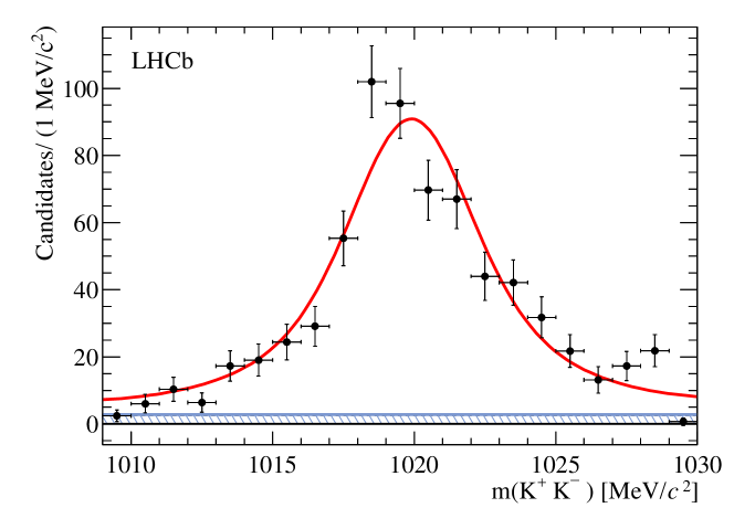
Figure 4: The $K^{+}K^{-}$ invariant mass distribution for background-subtracted ${{B}^{0}_{s}}\!\rightarrow\phi{{\pi}^{+}}{{\pi}^{-}}$ signal events with a fit to the dominant P-wave $\phi$ meson shown as a solid (red) line, and a small S-wave $K^{+}K^{-}$ contribution shown as a hatched (blue) area.

5 Amplitude Analysis

There are several resonances that can decay into a $\pi^{+}\pi^{-}$ final state in the region $400<m(\pi^{+}\pi^{-})<1600$${\mathrm{\,Me\kern-1.00006ptV\!/}c^{2}}$. These are listed in Table 1 together with the mass models used to describe them and the source of the model parameters. To study the resonant contributions, an amplitude analysis is performed using an unbinned maximum likelihood fit to the $m(\pi^{+}\pi^{-})$ mass and decay angle distributions of the ${B}^{0}_{s}$ candidates with their signal weights obtained by the sPlot technique. In the fit the uncertainties on the signal weights are taken into account in determining the uncertainties on the fitted amplitudes and phases.

Table 1: Possible resonances contributing to the $m(\pi^{+}\pi^{-})$ mass distribution. The shapes are either relativistic Breit-Wigner (BW) functions, or empirical threshold functions for the $f_{0}(500)$ proposed by Bugg [26] based on data from BES, and for the $f_{0}(980)$ proposed by Flatté [27] to account for the effect of the $K^{+}K^{-}$ threshold.

Resonance	Spin	Shape	Mass	Width	Source
$f_{0}(500)$	0	Bugg	400–800	Broad	BES [26]
$\rho$	1	BW	775	149	PDG [2]
$f_{0}(980)$	0	Flatté	980	40–100	LHCb [28]
$f_{2}(1270)$	2	BW	1275	185	PDG [2]
$f_{0}(1370)$	0	BW	1200–1500	200–500	PDG [2]
$f_{2}(1430)$	2	BW	1421	30	DM2 [29]
$\rho(1450)$	1	BW	1465	400	PDG [2]
$f_{0}(1500)$	0	BW	1461	124	LHCb [30]

Three decay angles are defined in the transversity basis as illustrated in Fig. 5, where $\theta_{1}$ is the $\pi^{+}\pi^{-}$ helicity angle between the $\pi^{+}$ direction in the $\pi^{+}\pi^{-}$ rest frame and the $\pi^{+}\pi^{-}$ direction in the $B$ rest frame, $\theta_{2}$ is the $K^{+}K^{-}$ helicity angle between the $K^{+}$ direction in the $\phi$ rest frame and the $\phi$ direction in the $B$ rest frame, and $\Phi$ is the acoplanarity angle between the $\pi^{+}\pi^{-}$ system and the $\phi$ meson decay planes.

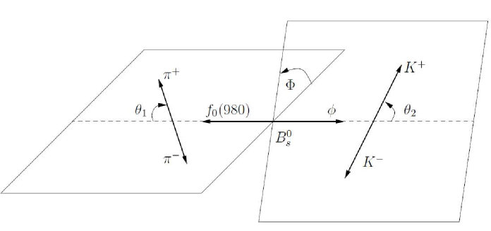
Figure 5: The definition of the decay angles $\theta_{1}$, $\theta_{2}$ and $\Phi$ for the decay ${{B}^{0}_{s}}\!\rightarrow\phi{{\pi}^{+}}{{\pi}^{-}}$ with $\phi\rightarrow K^{+}K^{-}$ and taking $f_{0}(980)\rightarrow\pi^{+}\pi^{-}$ for illustration.

The LHCb detector geometry and the kinematic selections on the final state particles lead to detection efficiencies that vary as a function of $m(\pi^{+}\pi^{-})$ and the decay angles. This is studied using simulated signal events, and is parameterised by a four-dimensional function using Legendre polynomials, taking into account the correlations between the variables. Figure 6 shows the projections of the detection efficiency and the function used to describe it. There is a significant drop of efficiency at $\cos\theta_{1}=\pm 1$, a smaller reduction of efficiency for $\cos\theta_{2}=\pm 1$, a flat efficiency in $\Phi$, and a monotonic efficiency increase with $m(\pi^{+}\pi^{-})$. This efficiency dependence is included in the amplitude fits.

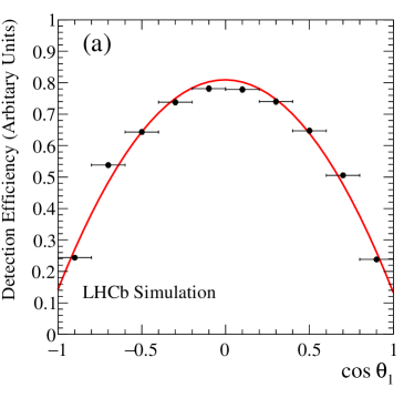
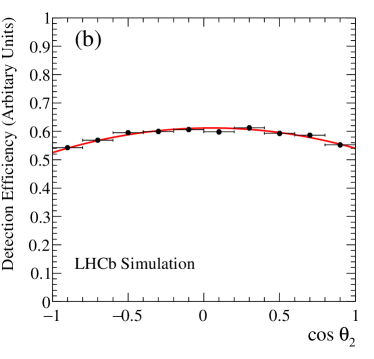
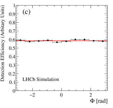
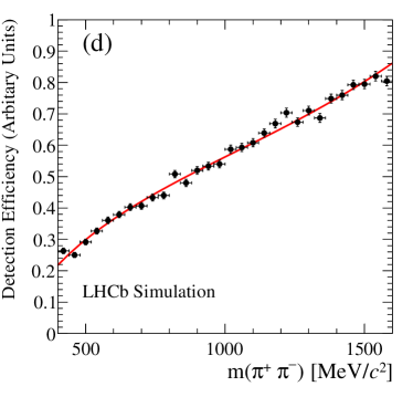
Figure 6: One-dimensional projections of the detection efficiency parameterised using Legendre polynomials (solid red lines) as a function of (a) $\cos\theta_{1}$, (b) $\cos\theta_{2}$, (c) $\Phi$ and (d) $m(\pi^{+}\pi^{-})$, superimposed on the efficiency determined from the ratio of the accepted/generated ${{B}^{0}_{s}}\!\rightarrow\phi{{\pi}^{+}}{{\pi}^{-}}$ events.

The decay rate for the mass range $m(\pi^{+}\pi^{-})<1100$${\mathrm{\,Me\kern-1.00006ptV\!/}c^{2}}$ can be described primarily by the S-wave and P-wave $\pi^{+}\pi^{-}$ contributions from the $f_{0}(980)$ and $\rho$ mesons. The S-wave contribution is parameterised by a single amplitude $A_{S}$. For the P-wave there are three separate amplitudes $A_{0}$, $A_{\perp}$ and $A_{\parallel}$ from the possible spin configurations of the final state vector mesons. The amplitudes $A_{j}$, where $j=(0,\perp,\parallel,S)$, are complex and can be written as $|A_{j}|e^{i\delta_{j}}$. By convention, the phase $\delta_{S}$ is chosen to be zero. In the region $m(\pi^{+}\pi^{-})>1100$${\mathrm{\,Me\kern-1.00006ptV\!/}c^{2}}$ the differential decay rate requires additional contributions from the D-wave $f_{2}(1270)$ meson and other possible resonances at higher mass.

The total differential decay rate is given by the square of the sum of the amplitudes. It can be written as

$$\frac{d^{4}\Gamma}{d\cos\theta_{1}d\cos\theta_{2}d\Phi dm_{\pi\pi}}=\frac{9}{8\pi}\sum_{i}T_{i}~{}f_{i}(\theta_{1},\theta_{2},\Phi)~{}\mathcal{M}_{i}(m_{\pi\pi})d\Omega_{4}(KK\pi\pi)\hskip 2.84544pt,$$ (1)

where the $T_{i}$ are either squares of the amplitudes $A_{j}$ or interference terms between them, $f_{i}$ are decay angle distributions, $\mathcal{M}_{i}$ are resonant $\pi^{+}\pi^{-}$ mass distributions and $d\Omega_{4}$ is the phase-space element for four-body decays. The detailed forms of these functions are given in Table 2 for the contributions from the $f_{0}(980)$, $\rho$ and $f_{2}(1270)$ resonances. Note that interference terms between $C\!P$-even amplitudes ($A_{0}$, $A_{\parallel}$, $A_{\perp}^{1270}$) and $C\!P$-odd amplitudes ($A_{S}$, $A_{\perp}$, $A_{0}^{1270}$, $A_{\parallel}^{1270}$), can be ignored in the sum of ${B}^{0}_{s}$ and ${\kern 1.79993pt\overline{\kern-1.79993ptB}{}}{}^{0}_{s}$ decays in the absence of $C\!P$ violation, as indicated by the measurements in the related decay ${{B}^{0}_{s}}\!\rightarrow\phi\phi$ [4]. With this assumption one $C\!P$-even phase $\delta_{\perp}^{1270}$ can also be chosen to be zero. The fit neglects the interference terms between P and D-waves, and the P-wave-only interference term ($i=4$ in Table 2), which are all found to be small when included in the fit. This leaves only a single P-wave phase $\delta_{\perp}$ and two D-wave phases $\delta_{\parallel}^{1270}$ and $\delta_{0}^{1270}$ to be fitted for these three resonant contributions.

Table 2: The individual terms $i=1$ to $i=6$ come from the S-wave and P-wave $\pi^{+}\pi^{-}$ amplitudes associated with the $f_{0}(980)$ and $\rho$, and the terms $i=7$ to $i=12$ come from the D-wave amplitudes associated with the $f_{2}(1270)$. See the text for definitions of $T_{i}$, $f_{i}$ and $\mathcal{M}_{i}$, and for a discussion of the interference terms omitted from this table.

$i$	$T_{i}$	$f_{i}$ ($\theta_{1},\theta_{2},\Phi$)	$\mathcal{M}_{i}(m_{\pi\pi})$
1	$|A_{0}|^{2}$	$\cos^{2}\theta_{1}\cos^{2}\theta_{2}$	$|M_{1}(m_{\pi\pi})|^{2}$
2	$|A_{\parallel}|^{2}$	$\frac{1}{4}\sin^{2}\theta_{1}\sin^{2}\theta_{2}(1+\cos 2\Phi)$	$|M_{1}(m_{\pi\pi})|^{2}$
3	$|A_{\perp}|^{2}$	$\frac{1}{4}\sin^{2}\theta_{1}\sin^{2}\theta_{2}(1-\cos 2\Phi)$	$|M_{1}(m_{\pi\pi})|^{2}$
4	$|A_{\parallel}A_{0}^{*}|$	$\sqrt{2}\cos\theta_{1}\sin\theta_{1}\cos\theta_{2}\sin\theta_{2}\cos\Phi$	$|M_{1}(m_{\pi\pi})|^{2}\cos(\delta_{\parallel}-\delta_{0})$
5	$|A_{S}|^{2}$	$\frac{1}{3}\cos^{2}\theta_{2}$	$|M_{0}(m_{\pi\pi})|^{2}$
6	$|A_{\perp}A_{S}^{*}|$	$\frac{\sqrt{6}}{3}\sin\theta_{1}\cos\theta_{2}\sin\theta_{2}\sin\Phi$	$\mathcal{R}e[M_{1}(m_{\pi\pi})M_{0}^{*}(m_{\pi\pi})e^{i\delta_{\perp}}]$
7	$|A_{0}^{1270}|^{2}$	$\frac{5}{12}(3\cos^{2}\theta_{1}-1)^{2}\cos^{2}\theta_{2}$	$|M_{2}(m_{\pi\pi})|^{2}$
8	$|A_{\parallel}^{1270}|^{2}$	$\frac{5}{2}\sin^{2}\theta_{1}\sin^{2}\theta_{2}\cos^{2}\theta_{1}\cos^{2}\Phi$	$|M_{2}(m_{\pi\pi})|^{2}$
9	$|A_{\perp}^{1270}|^{2}$	$\frac{5}{2}\sin^{2}\theta_{1}\sin^{2}\theta_{2}cos^{2}\theta_{1}\sin^{2}\Phi$	$|M_{2}(m_{\pi\pi})|^{2}$
10	$|A_{\parallel}^{1270}A_{0}^{1270*}|$	$\frac{5}{4\sqrt{6}}(3\cos^{2}\theta_{1}-1)\sin 2\theta_{1}\sin 2\theta_{2}\cos\Phi$	$|M_{2}(m_{\pi\pi})|^{2}\cos(\delta_{\parallel}^{1270}-\delta_{0}^{1270})$
11	$|A_{\parallel}^{1270}A_{S}^{*}|$	$\frac{\sqrt{10}}{3}\sin\theta_{1}\cos\theta_{1}\sin\theta_{2}\cos\theta_{2}\cos\Phi$	$\mathcal{R}e[M_{2}(m_{\pi\pi})M_{0}^{*}(m_{\pi\pi})e^{i\delta_{\parallel}^{1270}}]$
12	$|A_{0}^{1270}A_{S}^{*}|$	$\frac{\sqrt{5}}{3}(3\cos^{2}\theta_{1}-1)\cos^{2}\theta_{2}$	$\mathcal{R}e[M_{2}(m_{\pi\pi})M_{0}^{*}(m_{\pi\pi})e^{-i\delta_{0}^{1270}}]$

Several amplitude fits have been performed including different resonant contributions. All fits include the $f_{0}(980)$ and $f_{2}(1270)$ resonances. The high-mass region $1350<m(\pi^{+}\pi^{-})<1600$${\mathrm{\,Me\kern-1.00006ptV\!/}c^{2}}$ has been modelled by either an S-wave or a D-wave $\pi^{+}\pi^{-}$ contribution, where the masses and widths of these contributions are determined by the fits, but the shapes are constrained to be Breit-Wigner functions. In each case the respective terms in Table 2 from $f_{0}(980)$ or $f_{2}(1270)$ have to be duplicated for the higher resonance. For the higher S-wave contribution this introduces one new amplitude $A_{S}^{1500}$ and phase $\delta_{S}^{1500}$, and there is an additional interference term between the two S-wave resonances. For the higher D-wave contribution $f_{2}(1430)$ there are three new amplitudes and phases, and several interference terms between the two D-wave resonances. A contribution from the P-wave $\rho(1450)$ has also been considered, but is found to be negligible and is not included in the final fit. The fit quality has been assessed using a binned $\chi^{2}$ calculation based on the projected $\cos\theta_{1}$, $\cos\theta_{2}$ and $m(\pi^{+}\pi^{-})$ distributions. In the high-mass region the best fit uses an S-wave component with a fitted mass and width of $1427\pm 7$${\mathrm{\,Me\kern-1.00006ptV\!/}c^{2}}$ and $143\pm 17$${\mathrm{\,Me\kern-1.00006ptV\!/}c^{2}}$, hereafter referred to as the $f_{0}(1500)$ for convenience. The mass is lower than the accepted value of $1504\pm 6$${\mathrm{\,Me\kern-1.00006ptV\!/}c^{2}}$ for the $f_{0}(1500)$[2]. It is also lower than the equivalent S-wave component in ${{B}^{0}_{s}}\rightarrow{{J\mskip-3.0mu/\mskip-2.0mu\psi\mskip 2.0mu}}\pi^{+}\pi^{-}$ where the fitted mass and width were $1461\pm 3$${\mathrm{\,Me\kern-1.00006ptV\!/}c^{2}}$ and $124\pm 7$${\mathrm{\,Me\kern-1.00006ptV\!/}c^{2}}$ [30]. This may be due to the absence of contributions from the $\rho$ and $f_{2}(1270)$ in ${{B}^{0}_{s}}\rightarrow{{J\mskip-3.0mu/\mskip-2.0mu\psi\mskip 2.0mu}}\pi^{+}\pi^{-}$. It has been suggested [25, 31] that the observed $m(\pi^{+}\pi^{-})$ distributions can be described by an interference between the $f_{0}(1370)$ and $f_{0}(1500)$, but with the current statistics of the ${{B}^{0}_{s}}\!\rightarrow\phi{{\pi}^{+}}{{\pi}^{-}}$ sample it is not possible to verify this.

In the low-mass region $m(\pi^{+}\pi^{-})<900$${\mathrm{\,Me\kern-1.00006ptV\!/}c^{2}}$ the effect of adding a contribution from the $\rho$ is studied. The $\rho$ contribution significantly improves the fit quality and has a statistical significance of $4.5\sigma$, estimated by running pseudo-experiments. A contribution from the $f_{0}(500)$ has been considered as part of the systematics. The preferred fit, including the $\rho$, $f_{0}(980)$, $f_{2}(1270)$ and $f_{0}(1500)$, has $\chi^{2}/\mathrm{ndf}=34/20$. Removing the $\rho$ increases this to $\chi^{2}/\mathrm{ndf}=53/24$, and replacing the S-wave $f_{0}(1500)$ with a D-wave $f_{2}(1430)$ increases it to $\chi^{2}/\mathrm{ndf}=78/16$. The projections of the preferred fit, including the $\rho$, $f_{0}(980)$, $f_{2}(1270)$ and $f_{0}(1500)$, are shown in Fig. 7. The fitted amplitudes and phases are given in Table 3. From Fig. 7 it can be seen that the low numbers of observed candidates in the regions $|\cos\theta_{1}|>0.8$ and $|\cos\theta_{2}|<0.4$ require a large S-wave $\pi^{+}\pi^{-}$ contribution, and smaller P-wave and D-wave contributions.

Table 3: The resonance amplitudes and phases from the preferred fit to the $m(\pi^{+}\pi^{-})$ and decay angle distributions of the ${B}^{0}_{s}$ candidates, including the $\rho$, $f_{0}(980)$, $f_{2}(1270)$ and $f_{0}(1500)$. See text for definitions of the amplitudes and phases.

Amplitude	Fit value	Phase	Fit value (rad)
$A_{0}$	$0.212\pm 0.035$
$A_{\parallel}$	$0.049\pm 0.031$
$A_{\perp}$	$0.168\pm 0.026$	$\delta_{\perp}$	$+1.90\pm 0.28$
$A_{S}$	$0.603\pm 0.036$
$A_{0}^{1270}$	$0.295\pm 0.058$	$\delta_{0}^{1270}$	$-0.62\pm 0.18$
$A_{\parallel}^{1270}$	$0.203\pm 0.042$	$\delta_{\parallel}^{1270}$	$+1.26\pm 0.25$
$A_{\perp}^{1270}$	$0.261\pm 0.037$
$A_{S}^{1500}$	$0.604\pm 0.031$	$\delta_{S}^{1500}$	$+3.14\pm 0.30$

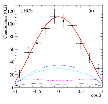
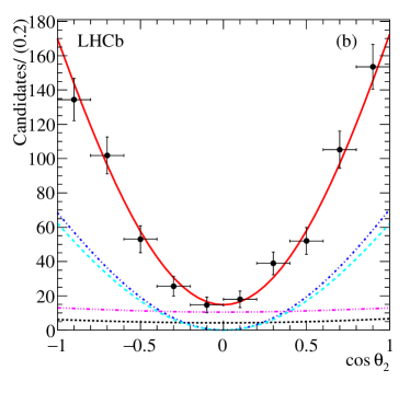
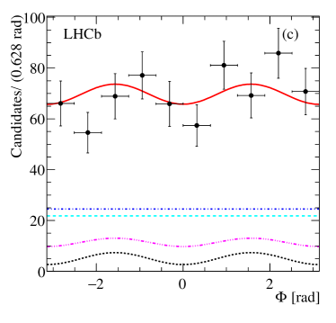
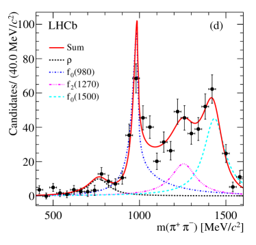
Figure 7: Projections of (a) $\cos\theta_{1}$, (b) $\cos\theta_{2}$, (c) $\Phi$, and (d) $m(\pi^{+}\pi^{-})$ for the preferred fit. The $\rho$ contribution is shown by the dotted (black) line, the $f_{0}(980)$ by the dot-dashed (blue) line, the $f_{2}(1270)$ by the double-dot-dashed (magenta) line and the $f_{0}(1500)$ by the dashed (cyan) line. Note that the expected distributions from each resonance include the effect of the experimental efficiency. The solid (red) line shows the total fit. The points with error bars are the data, where the background has been subtracted using the ${B}^{0}_{s}$ signal weights from the $K^{+}K^{-}\pi^{+}\pi^{-}$ invariant mass fit.

To convert the fitted amplitudes into fractional contributions from different resonances they need to be first summed over the different polarisations and then squared. Interference terms between the resonances are small, but not completely negligible. When calculating the fit fractions and event yields, the interference terms are included in the total yield but not in the individual resonance yields. As a consequence, the sum of the fractions is not 100%. Table 4 gives the fit fractions and the corresponding event yields for the resonant contributions to the ${{B}^{0}_{s}}\!\rightarrow\phi{{\pi}^{+}}{{\pi}^{-}}$ decay for the fits with and without a $\rho$.

Table 4: Fit fractions in % and event yields for the resonances contributing to ${{B}^{0}_{s}}\!\rightarrow\phi{{\pi}^{+}}{{\pi}^{-}}$. Results are quoted for the preferred model with a $\rho$, and for an alternative model without a $\rho$ which is used to evaluate systematic uncertainties.

Resonance	Fit fractions %		Event yields
contribution	without $\rho$	with $\rho$	without $\rho$	with $\rho$
$\rho$	–	7.1 $\pm$ 1.5	–	50 $\pm$ 11
$f_{0}(980)$	39.5 $\pm$ 2.9	35.6 $\pm$ 4.3	274 $\pm$ 23	247 $\pm$ 31
$f_{2}(1270)$	23.5 $\pm$ 2.7	15.1 $\pm$ 3.2	163 $\pm$ 20	112 $\pm$ 23
$f_{0}(1500)$	26.5 $\pm$ 2.2	34.7 $\pm$ 3.4	184 $\pm$ 17	241 $\pm$ 26

6 Determination of branching fractions

The branching fractions are determined using the relationship

$$\frac{\mathcal{B}({{B}^{0}_{s}}({{B}^{0}})\rightarrow\phi\pi^{+}\pi^{-})}{\mathcal{B}(B_{s}^{0}\rightarrow\phi\phi)}=\frac{N(\phi\pi^{+}\pi^{-})}{N(\phi\phi)}\times\frac{\varepsilon^{tot}_{\phi\phi}}{\varepsilon^{tot}_{\phi\pi^{+}\pi^{-}}}\times\frac{f_{s}}{f_{d}}\times\mathcal{B}(\phi\rightarrow K^{+}K^{-})\times f_{P}\hskip 2.84544pt.$$

The signal yields $N(\phi\pi^{+}\pi^{-})$ for the inclusive modes are taken from the fit to the $K^{+}K^{-}\pi^{+}\pi^{-}$ mass distribution in Fig. 2, and for the normalisation mode $N(\phi\phi)$ is taken from the fit to the $K^{+}K^{-}K^{+}K^{-}$ mass distribution in Fig. 3. The factor $f_{P}=(93\pm 4)$% corrects for the difference in the fitted S-wave $K^{+}K^{-}$ contributions to the $K^{+}K^{-}$ mass distribution around the nominal $\phi$ mass between the signal and normalisation modes. The branching fraction $\mathcal{B}(\phi\rightarrow K^{+}K^{-})=(48.9\pm 0.5)\%$[2] enters twice in the normalisation mode. The factor $f_{s}/f_{d}=0.259\pm 0.015$[32] only applies to the ${{B}^{0}}\!\rightarrow\phi{{\pi}^{+}}{{\pi}^{-}}$ mode in the above ratio, but also appears in the ratio of ${{B}^{0}_{s}}\!\rightarrow\phi\phi$ relative to ${{B}^{0}}\rightarrow\phi{{K}^{*}}$, so it effectively cancels out in the determination of the ${{B}^{0}}\!\rightarrow\phi{{\pi}^{+}}{{\pi}^{-}}$ branching fraction. For the ${{B}^{0}_{s}}\!\rightarrow\phi{{\pi}^{+}}{{\pi}^{-}}$ mode it is included in the determination of $\mathcal{B}({{B}^{0}_{s}}\!\rightarrow\phi\phi)$ [7]. The total selection efficiencies $\varepsilon^{{\rm tot}}_{\phi\pi^{+}\pi^{-}}$ and $\varepsilon^{{\rm tot}}_{\phi\phi}$ are given in Table 5.

For the inclusive modes the branching fractions with $400<m(\pi^{+}\pi^{-})<1600{\mathrm{\,Me\kern-1.00006ptV\!/}c^{2}}$ are

$${\cal{B}}({{B}^{0}_{s}}\!\rightarrow\phi{{\pi}^{+}}{{\pi}^{-}})=[3.48\pm 0.23]\times 10^{-6}\hskip 2.84544pt,$$

and

$${\cal{B}}({{B}^{0}}\!\rightarrow\phi{{\pi}^{+}}{{\pi}^{-}})=[1.82\pm 0.25]\times 10^{-7}\hskip 2.84544pt,$$

where the quoted uncertainties are purely statistical, but include the uncertainties on the yield of the normalisation mode, and on the S-wave $K^{+}K^{-}$ contributions to the signal and normalisation modes. For the exclusive ${B}^{0}_{s}$ modes the signal yields are taken from the final column in Table 4. The branching fractions are

$${\cal{B}}({{B}^{0}_{s}}\!\rightarrow\phi f_{0}(980))=[1.12\pm 0.16]\times 10^{-6}\hskip 2.84544pt,$$

$${\cal{B}}({{B}^{0}_{s}}\rightarrow\phi f_{2}(1270))=[0.61\pm 0.13]\times 10^{-6}\hskip 2.84544pt,$$

and

$${\cal{B}}({{B}^{0}_{s}}\!\rightarrow\phi\rho^{0})=[2.7\pm 0.6]\times 10^{-7}\hskip 2.84544pt.$$

The remaining $1.5\times 10^{-6}$ of the inclusive ${{B}^{0}_{s}}$ branching fraction is mostly accounted for by an S-wave contribution in the region $1350-1600{\mathrm{\,Me\kern-1.00006ptV\!/}c^{2}}$ as discussed in the previous section.

Table 5: Selection efficiencies for the signal and normalisation modes in %, as determined from simulated event samples. Here “Initial selection” refers to a loose set of requirements on the four tracks forming the $B$ candidate. The “Offline selection” includes the charm and $\phi K^{*}{{}^{0}}$ vetoes, as well as the BDT. Angular acceptance and decay time refer to corrections made for the incorrect modelling of these distributions in the inclusive and ${{B}^{0}_{s}}\!\rightarrow\phi f_{0}(980)$ simulated event samples.

Efficiency	${{B}^{0}_{s}}({{B}^{0}})\rightarrow\phi\pi^{+}\pi^{-}$	$B_{s}^{0}\rightarrow\phi\rho^{0}$	${{B}^{0}_{s}}\!\rightarrow\phi f_{0}(980)$	${{B}^{0}_{s}}\!\rightarrow\phi\phi$
Detector acceptance	17.4	18.1	18.0	17.1
Initial selection	8.43	7.35	8.48	14.6
Trigger	34.9	34.9	34.5	28.6
Offline selection	63.9 (57.1)	62.5	63.2	59.3
Particle identification	87.5	87.5	87.5	93.9
Angular acceptance	95.9 (100)	100	100	100
Decay time	100	100	104.5	100
Total	0.275 (0.256)	0.254	0.303	0.398

7 Systematic uncertainties

Many systematic effects cancel in the ratio of efficiencies between the signal and normalisation modes. The remaining systematic uncertainties in the determination of the branching fractions come from replacing the $\pi^{+}\pi^{-}$ pair with a second $\phi$ meson decaying to two kaons. The systematic uncertainties are summarised in Table 6.

The trigger selection has a different performance for the ${{B}^{0}_{s}}\rightarrow\phi\pi^{+}\pi^{-}$ signal and for the ${{B}^{0}_{s}}\rightarrow\phi\phi$ normalisation mode due to the different kinematics of the final state hadrons. The simulation of the trigger does not reproduce this difference accurately for hadronic decays, and a ${{D}^{0}}\rightarrow K^{-}\pi^{+}$ control sample, collected with a minimum bias trigger, is used to evaluate corrections to the trigger efficiencies between the simulation and the data. These are applied as per-event reweightings of the simulation as a function of track $p_{T}$, particle type $K$ or $\pi$, and magnetic field orientation. For both the signal and normalisation modes there are large corrections of $\approx 30$%, but they almost completely cancel in the ratio, leaving a systematic uncertainty of 0.5% from this source.

Another aspect of the detector efficiency that is not accurately modelled by the simulation is hadronic interactions in the detector. A sample of simulated ${{B}^{0}}\rightarrow{{J\mskip-3.0mu/\mskip-2.0mu\psi\mskip 2.0mu}}{{K}^{*}}^{0}$ events is used to determine the fraction of kaons and pions that interact within the detector as a function of their momentum. On average this varies from 11% for $K^{+}$ to 15% for $\pi^{-}$. These numbers are then scaled up to account for additional material in the detector compared to the simulation. The effect partly cancels in the ratio of the signal and normalisation modes leaving a 0.5% systematic uncertainty from this source.

The offline selection efficiency has an uncertainty coming from the performance of the multivariate BDT. This has been studied by varying the selection on the ${{B}^{0}_{s}}\!\rightarrow\phi\phi$ normalisation mode, and extracting the shapes of the input variables from data using the sPlot technique. The distributions agree quite well between simulation and data, but there are small differences. When these are propagated to the signal modes they lead to a reduction in the BDT efficiency. Again the effect partially cancels in the ratio leaving a systematic uncertainty of 2.3%.

The offline selection also has an uncertainty coming from the different particle identification criteria used for the $\pi^{+}\pi^{-}$ in the signal and the $K^{+}K^{-}$ from the second $\phi$ in the normalisation mode. Corrections between simulation and data are studied using calibration samples, with kaons and pions binned in $p_{T}$, $\eta$ and number of tracks in the event. There is an uncertainty of 0.1% from the size of the calibration samples. Using different binning schemes for the corrections leads to a slightly higher estimate for the systematic uncertainty of 0.3%.

For the angular acceptance there is an uncertainty in the $m(\pi^{+}\pi^{-})$ and angular distributions for the inclusive decays, and in the polarisations of the $\rho^{0}$ and $f_{2}(1270)$. A three-dimensional binning in $[\cos\theta_{1},\cos\theta_{2},m(\pi^{+}\pi^{-})]$ is used to reweight the simulation to match the data distributions for these modes. The accuracy of this procedure is limited by the number of bins and hence by the data statistics. By varying the binning scheme systematic uncertainties of 3.8% (10.7%) are determined for ${{B}^{0}_{s}}$ (${{B}^{0}}$) from this reweighting procedure. The larger ${{B}^{0}}$ uncertainty reflects the smaller signal yield. The angular distribution of the ${{B}^{0}_{s}}\rightarrow\phi\phi$ normalisation mode is modelled according to the published LHCb measurements [4], which introduces a negligible uncertainty.

The decay time acceptance of the detector falls off rapidly at short decay times due to the requirement that the tracks are consistent with coming from a secondary vertex. For ${B}^{0}_{s}$ decays the decay time distribution is modelled by the flavour-specific lifetime, but it should be modelled by a combination of the heavy and light mass eigenstates, depending on the decay mode. A systematic uncertainty of 1.1% is found when replacing the flavour-specific lifetime by the lifetime of the heavy eigenstate and determining the change in the decay time acceptance. There is no effect on ${B}^{0}$ decays or on the normalisation mode where the lifetime is modelled according to the published measurements.

The $K^{+}K^{-}\pi^{+}\pi^{-}$ and $K^{+}K^{-}K^{+}K^{-}$ invariant mass fits are repeated using a single Gaussian and using a power-law function to model the tails of the signal shapes. For the $m(K^{+}K^{-}\pi^{+}\pi^{-})$ fit contributions from partially reconstructed backgrounds are added, including ${{B}^{0}_{s}}\rightarrow\phi\phi(\pi^{+}\pi^{-}\pi^{0})$ and ${{B}^{0}_{s}}\rightarrow\phi\eta^{\prime}(\pi^{+}\pi^{-}\gamma)$. These changes lead to uncertainties on the ${{B}^{0}_{s}}$ (${{B}^{0}}$) yields of 1.2% (19.5%). The large uncertainty on the ${B}^{0}$ yield comes both from the change in the signal shape and from the addition of partially reconstructed ${B}^{0}_{s}$ backgrounds. This systematic uncertainty reduces the significance of the ${B}^{0}$ signal from $7.7\sigma$ to $4.5\sigma$.

The results of the amplitude analysis for the exclusive ${{B}^{0}_{s}}$ decays depend on the set of input resonances that are used. The effect of including the $\rho^{0}$ is treated as a systematic uncertainty on the $f_{0}(980)$ and $f_{2}(1270)$ yields (see Table 4). The effect of adding either an $f_{0}(500)$ or a $\rho(1450)$ is treated as a systematic uncertainty on all the exclusive modes.

The difference between the S-wave $K^{+}K^{-}$ components in the signal and normalisation modes is measured to be $(7.1\pm 4.0)$% from fits to the $K^{+}K^{-}$ mass distributions. The uncertainty on this is treated as part of the statistical error. However, the S-wave component of the signal sample was not included in the amplitude analysis where it would give a flat distribution in $\cos\theta_{2}$. A study of the dependence of the S-wave $K^{+}K^{-}$ component as a function of $m(\pi^{+}\pi^{-})$ does not indicate a significant variation, and the statistical uncertainty of 6% from this study is taken as a systematic uncertainty on the yields of the exclusive modes extracted from the amplitude analysis.

Table 6: Systematic uncertainties in % on the branching fractions of ${B}^{0}_{s}$ and ${B}^{0}$ decays. All the uncertainties are taken on the ratio of the signal to the normalisation mode. Uncertainties marked by a dash are either negligible or exactly zero. The asymmetric uncertainties on $\phi f_{0}(980)$ and $\phi f_{2}(1270)$ come from the differences in yields between the fits with and without the $\rho^{0}$ contribution.

Systematic	$B_{s}^{0}\rightarrow\phi\rho^{0}$	${{B}^{0}_{s}}\!\rightarrow\phi f_{0}(980)$	$B_{s}^{0}\rightarrow\phi f_{2}(1270)$	${{B}^{0}_{s}}({{B}^{0}})\rightarrow\phi\pi^{+}\pi^{-}$
Trigger	0.5	0.5	0.5	0.5
Hadronic interactions	0.5	0.5	0.5	0.5
Offline selection	2.3	2.3	2.3	2.3
Particle identification	0.3	0.3	0.3	0.3
Angular acceptance	3.8	$-$	3.8	3.8 (10.7)
Decay time acceptance	1.1	1.1	1.1	1.1 ($-$)
$m(K^{+}K^{-}\pi^{+}\pi^{-})$ fit	1.2	1.2	1.2	1.2 (19.5)
Amplitude analysis	2.5	$+4.7/-0.4$	$+17.6/-2.7$	$-$
S-wave $K^{+}K^{-}$	6.0	6.0	6.0	$-$
Total	7.0	$+8.2/-6.7$	$+19.2/-8.1$	4.8 (22.4)

8 Summary and conclusions

This paper reports the first observation of the inclusive decay ${{B}^{0}_{s}}\!\rightarrow\phi{{\pi}^{+}}{{\pi}^{-}}$. The branching fraction in the mass range $400<m(\pi^{+}\pi^{-})<1600$${\mathrm{\,Me\kern-1.00006ptV\!/}c^{2}}$ is measured to be

$$\mathcal{B}({{B}^{0}_{s}}\!\rightarrow\phi{{\pi}^{+}}{{\pi}^{-}})=[3.48\pm 0.23\pm 0.17\pm 0.35]\times 10^{-6}\;,$$

where the first uncertainty is statistical, the second is systematic, and the third is due to the normalisation mode ${{B}^{0}_{s}}\!\rightarrow\phi\phi$.

Evidence is also seen for the inclusive decay ${{B}^{0}}\!\rightarrow\phi{{\pi}^{+}}{{\pi}^{-}}$ with a statistical significance of 7.7$\sigma$, which is reduced to 4.5$\sigma$ after taking into account the systematic uncertainties on the signal yield. The branching fraction in the mass range $400<m(\pi^{+}\pi^{-})<1600$${\mathrm{\,Me\kern-1.00006ptV\!/}c^{2}}$ is

$$\mathcal{B}({{B}^{0}}\!\rightarrow\phi{{\pi}^{+}}{{\pi}^{-}})=[1.82\pm 0.25\pm 0.41\pm 0.14]\times 10^{-7}\;.$$

An amplitude analysis is used to separate out exclusive contributions to the ${B}^{0}_{s}$ decays. The decay ${{B}^{0}_{s}}\!\rightarrow\phi f_{0}(980)$ is observed with a significance of $8\,\sigma$, and the product branching fraction is

$$\mathcal{B}({{B}^{0}_{s}}\!\rightarrow\phi f_{0}(980),f_{0}(980)\rightarrow\pi^{+}\pi^{-})=[1.12\pm 0.16^{+0.09}_{-0.08}\pm 0.11]\times 10^{-6}\;.$$

The decay $B_{s}^{0}\rightarrow\phi f_{2}(1270)$ is observed with a significance of $5\,\sigma$, and the product branching fraction is

$$\mathcal{B}(B_{s}^{0}\rightarrow\phi f_{2}(1270),f_{2}(1270)\rightarrow\pi^{+}\pi^{-})=[0.61\pm 0.13^{+0.12}_{-0.05}\pm 0.06]\times 10^{-6}\,.$$

There is also a contribution from higher mass S-wave $\pi^{+}\pi^{-}$ states in the region $1350-1600{\mathrm{\,Me\kern-1.00006ptV\!/}c^{2}}$, which could be ascribed to a linear superposition of the $f_{0}(1370)$ and the $f_{0}(1500)$. There is $4\sigma$ evidence for the decay ${{B}^{0}_{s}}\!\rightarrow\phi\rho^{0}$ with a branching fraction of

$$\mathcal{B}({{B}^{0}_{s}}\!\rightarrow\phi\rho^{0})=[2.7\pm 0.7\pm 0.2\pm 0.2]\times 10^{-7}\,.$$

This is lower than the Standard Model prediction of $[4.4^{+2.2}_{-0.7}]\times 10^{-7}$, but still consistent with it, and provides a constraint on possible contributions from new physics in this decay.

With more data coming from the LHC it will be possible to further investigate the exclusive decays, perform an amplitude analysis of the ${B}^{0}$ decays, and eventually make measurements of time-dependent $C\!P$ violation that are complementary to the measurements already made in the ${{B}^{0}_{s}}\!\rightarrow\phi\phi$ decay.

9 Acknowledgements

We express our gratitude to our colleagues in the CERN accelerator departments for the excellent performance of the LHC. We thank the technical and administrative staff at the LHCb institutes. We acknowledge support from CERN and from the national agencies: CAPES, CNPq, FAPERJ and FINEP (Brazil); NSFC (China); CNRS/IN2P3 (France); BMBF, DFG and MPG (Germany); INFN (Italy); FOM and NWO (The Netherlands); MNiSW and NCN (Poland); MEN/IFA (Romania); MinES and FASO (Russia); MinECo (Spain); SNSF and SER (Switzerland); NASU (Ukraine); STFC (United Kingdom); NSF (USA). We acknowledge the computing resources that are provided by CERN, IN2P3 (France), KIT and DESY (Germany), INFN (Italy), SURF (The Netherlands), PIC (Spain), GridPP (United Kingdom), RRCKI and Yandex LLC (Russia), CSCS (Switzerland), IFIN-HH (Romania), CBPF (Brazil), PL-GRID (Poland) and OSC (USA). We are indebted to the communities behind the multiple open source software packages on which we depend. Individual groups or members have received support from AvH Foundation (Germany), EPLANET, Marie Skłodowska-Curie Actions and ERC (European Union), Conseil Général de Haute-Savoie, Labex ENIGMASS and OCEVU, Région Auvergne (France), RFBR and Yandex LLC (Russia), GVA, XuntaGal and GENCAT (Spain), Herchel Smith Fund, The Royal Society, Royal Commission for the Exhibition of 1851 and the Leverhulme Trust (United Kingdom).

LHCb collaboration

R. Aaij⁴⁰, B. Adeva³⁹, M. Adinolfi⁴⁸, Z. Ajaltouni⁵, S. Akar⁶, J. Albrecht¹⁰, F. Alessio⁴⁰, M. Alexander⁵³, S. Ali⁴³, G. Alkhazov³¹, P. Alvarez Cartelle⁵⁵, A.A. Alves Jr⁵⁹, S. Amato², S. Amerio²³, Y. Amhis⁷, L. An⁴¹, L. Anderlini¹⁸, G. Andreassi⁴¹, M. Andreotti^17,g, J.E. Andrews⁶⁰, R.B. Appleby⁵⁶, F. Archilli⁴³, P. d’Argent¹², J. Arnau Romeu⁶, A. Artamonov³⁷, M. Artuso⁶¹, E. Aslanides⁶, G. Auriemma²⁶, M. Baalouch⁵, I. Babuschkin⁵⁶, S. Bachmann¹², J.J. Back⁵⁰, A. Badalov³⁸, C. Baesso⁶², S. Baker⁵⁵, W. Baldini¹⁷, R.J. Barlow⁵⁶, C. Barschel⁴⁰, S. Barsuk⁷, W. Barter⁴⁰, M. Baszczyk²⁷, V. Batozskaya²⁹, B. Batsukh⁶¹, V. Battista⁴¹, A. Bay⁴¹, L. Beaucourt⁴, J. Beddow⁵³, F. Bedeschi²⁴, I. Bediaga¹, L.J. Bel⁴³, V. Bellee⁴¹, N. Belloli^21,i, K. Belous³⁷, I. Belyaev³², E. Ben-Haim⁸, G. Bencivenni¹⁹, S. Benson⁴³, J. Benton⁴⁸, A. Berezhnoy³³, R. Bernet⁴², A. Bertolin²³, F. Betti¹⁵, M.-O. Bettler⁴⁰, M. van Beuzekom⁴³, Ia. Bezshyiko⁴², S. Bifani⁴⁷, P. Billoir⁸, T. Bird⁵⁶, A. Birnkraut¹⁰, A. Bitadze⁵⁶, A. Bizzeti^18,u, T. Blake⁵⁰, F. Blanc⁴¹, J. Blouw^11,†, S. Blusk⁶¹, V. Bocci²⁶, T. Boettcher⁵⁸, A. Bondar^36,w, N. Bondar^31,40, W. Bonivento¹⁶, A. Borgheresi^21,i, S. Borghi⁵⁶, M. Borisyak³⁵, M. Borsato³⁹, F. Bossu⁷, M. Boubdir⁹, T.J.V. Bowcock⁵⁴, E. Bowen⁴², C. Bozzi^17,40, S. Braun¹², M. Britsch¹², T. Britton⁶¹, J. Brodzicka⁵⁶, E. Buchanan⁴⁸, C. Burr⁵⁶, A. Bursche², J. Buytaert⁴⁰, S. Cadeddu¹⁶, R. Calabrese^17,g, M. Calvi^21,i, M. Calvo Gomez^38,m, A. Camboni³⁸, P. Campana¹⁹, D. Campora Perez⁴⁰, D.H. Campora Perez⁴⁰, L. Capriotti⁵⁶, A. Carbone^15,e, G. Carboni^25,j, R. Cardinale^20,h, A. Cardini¹⁶, P. Carniti^21,i, L. Carson⁵², K. Carvalho Akiba², G. Casse⁵⁴, L. Cassina^21,i, L. Castillo Garcia⁴¹, M. Cattaneo⁴⁰, Ch. Cauet¹⁰, G. Cavallero²⁰, R. Cenci^24,t, M. Charles⁸, Ph. Charpentier⁴⁰, G. Chatzikonstantinidis⁴⁷, M. Chefdeville⁴, S. Chen⁵⁶, S.-F. Cheung⁵⁷, V. Chobanova³⁹, M. Chrzaszcz^42,27, X. Cid Vidal³⁹, G. Ciezarek⁴³, P.E.L. Clarke⁵², M. Clemencic⁴⁰, H.V. Cliff⁴⁹, J. Closier⁴⁰, V. Coco⁵⁹, J. Cogan⁶, E. Cogneras⁵, V. Cogoni^16,40,f, L. Cojocariu³⁰, G. Collazuol^23,o, P. Collins⁴⁰, A. Comerma-Montells¹², A. Contu⁴⁰, A. Cook⁴⁸, S. Coquereau³⁸, G. Corti⁴⁰, M. Corvo^17,g, C.M. Costa Sobral⁵⁰, B. Couturier⁴⁰, G.A. Cowan⁵², D.C. Craik⁵², A. Crocombe⁵⁰, M. Cruz Torres⁶², S. Cunliffe⁵⁵, R. Currie⁵⁵, C. D’Ambrosio⁴⁰, E. Dall’Occo⁴³, J. Dalseno⁴⁸, P.N.Y. David⁴³, A. Davis⁵⁹, O. De Aguiar Francisco², K. De Bruyn⁶, S. De Capua⁵⁶, M. De Cian¹², J.M. De Miranda¹, L. De Paula², M. De Serio^14,d, P. De Simone¹⁹, C.-T. Dean⁵³, D. Decamp⁴, M. Deckenhoff¹⁰, L. Del Buono⁸, M. Demmer¹⁰, D. Derkach³⁵, O. Deschamps⁵, F. Dettori⁴⁰, B. Dey²², A. Di Canto⁴⁰, H. Dijkstra⁴⁰, F. Dordei⁴⁰, M. Dorigo⁴¹, A. Dosil Suárez³⁹, A. Dovbnya⁴⁵, K. Dreimanis⁵⁴, L. Dufour⁴³, G. Dujany⁵⁶, K. Dungs⁴⁰, P. Durante⁴⁰, R. Dzhelyadin³⁷, A. Dziurda⁴⁰, A. Dzyuba³¹, N. Déléage⁴, S. Easo⁵¹, M. Ebert⁵², U. Egede⁵⁵, V. Egorychev³², S. Eidelman^36,w, S. Eisenhardt⁵², U. Eitschberger¹⁰, R. Ekelhof¹⁰, L. Eklund⁵³, Ch. Elsasser⁴², S. Ely⁶¹, S. Esen¹², H.M. Evans⁴⁹, T. Evans⁵⁷, A. Falabella¹⁵, N. Farley⁴⁷, S. Farry⁵⁴, R. Fay⁵⁴, D. Fazzini^21,i, D. Ferguson⁵², V. Fernandez Albor³⁹, A. Fernandez Prieto³⁹, F. Ferrari^15,40, F. Ferreira Rodrigues¹, M. Ferro-Luzzi⁴⁰, S. Filippov³⁴, R.A. Fini¹⁴, M. Fiore^17,g, M. Fiorini^17,g, M. Firlej²⁸, C. Fitzpatrick⁴¹, T. Fiutowski²⁸, F. Fleuret^7,b, K. Fohl⁴⁰, M. Fontana¹⁶, F. Fontanelli^20,h, D.C. Forshaw⁶¹, R. Forty⁴⁰, V. Franco Lima⁵⁴, M. Frank⁴⁰, C. Frei⁴⁰, J. Fu^22,q, E. Furfaro^25,j, C. Färber⁴⁰, A. Gallas Torreira³⁹, D. Galli^15,e, S. Gallorini²³, S. Gambetta⁵², M. Gandelman², P. Gandini⁵⁷, Y. Gao³, L.M. Garcia Martin⁶⁸, J. García Pardiñas³⁹, J. Garra Tico⁴⁹, L. Garrido³⁸, P.J. Garsed⁴⁹, D. Gascon³⁸, C. Gaspar⁴⁰, L. Gavardi¹⁰, G. Gazzoni⁵, D. Gerick¹², E. Gersabeck¹², M. Gersabeck⁵⁶, T. Gershon⁵⁰, Ph. Ghez⁴, S. Gianì⁴¹, V. Gibson⁴⁹, O.G. Girard⁴¹, L. Giubega³⁰, K. Gizdov⁵², V.V. Gligorov⁸, D. Golubkov³², A. Golutvin^55,40, A. Gomes^1,a, I.V. Gorelov³³, C. Gotti^21,i, M. Grabalosa Gándara⁵, R. Graciani Diaz³⁸, L.A. Granado Cardoso⁴⁰, E. Graugés³⁸, E. Graverini⁴², G. Graziani¹⁸, A. Grecu³⁰, P. Griffith⁴⁷, L. Grillo^21,i, B.R. Gruberg Cazon⁵⁷, O. Grünberg⁶⁶, E. Gushchin³⁴, Yu. Guz³⁷, T. Gys⁴⁰, C. Göbel⁶², T. Hadavizadeh⁵⁷, C. Hadjivasiliou⁵, G. Haefeli⁴¹, C. Haen⁴⁰, S.C. Haines⁴⁹, S. Hall⁵⁵, B. Hamilton⁶⁰, X. Han¹², S. Hansmann-Menzemer¹², N. Harnew⁵⁷, S.T. Harnew⁴⁸, J. Harrison⁵⁶, M. Hatch⁴⁰, J. He⁶³, T. Head⁴¹, A. Heister⁹, K. Hennessy⁵⁴, P. Henrard⁵, L. Henry⁸, J.A. Hernando Morata³⁹, E. van Herwijnen⁴⁰, M. Heß⁶⁶, A. Hicheur², D. Hill⁵⁷, C. Hombach⁵⁶, H. Hopchev⁴¹, W. Hulsbergen⁴³, T. Humair⁵⁵, M. Hushchyn³⁵, N. Hussain⁵⁷, D. Hutchcroft⁵⁴, M. Idzik²⁸, P. Ilten⁵⁸, R. Jacobsson⁴⁰, A. Jaeger¹², J. Jalocha⁵⁷, E. Jans⁴³, A. Jawahery⁶⁰, F. Jiang³, M. John⁵⁷, D. Johnson⁴⁰, C.R. Jones⁴⁹, C. Joram⁴⁰, B. Jost⁴⁰, N. Jurik⁶¹, S. Kandybei⁴⁵, W. Kanso⁶, M. Karacson⁴⁰, J.M. Kariuki⁴⁸, S. Karodia⁵³, M. Kecke¹², M. Kelsey⁶¹, I.R. Kenyon⁴⁷, M. Kenzie⁴⁰, T. Ketel⁴⁴, E. Khairullin³⁵, B. Khanji^21,40,i, C. Khurewathanakul⁴¹, T. Kirn⁹, S. Klaver⁵⁶, K. Klimaszewski²⁹, S. Koliiev⁴⁶, M. Kolpin¹², I. Komarov⁴¹, R.F. Koopman⁴⁴, P. Koppenburg⁴³, A. Kozachuk³³, M. Kozeiha⁵, L. Kravchuk³⁴, K. Kreplin¹², M. Kreps⁵⁰, P. Krokovny^36,w, F. Kruse¹⁰, W. Krzemien²⁹, W. Kucewicz^27,l, M. Kucharczyk²⁷, V. Kudryavtsev^36,w, A.K. Kuonen⁴¹, K. Kurek²⁹, T. Kvaratskheliya^32,40, D. Lacarrere⁴⁰, G. Lafferty^56,40, A. Lai¹⁶, D. Lambert⁵², G. Lanfranchi¹⁹, C. Langenbruch⁹, T. Latham⁵⁰, C. Lazzeroni⁴⁷, R. Le Gac⁶, J. van Leerdam⁴³, J.-P. Lees⁴, A. Leflat^33,40, J. Lefrançois⁷, R. Lefèvre⁵, F. Lemaitre⁴⁰, E. Lemos Cid³⁹, O. Leroy⁶, T. Lesiak²⁷, B. Leverington¹², Y. Li⁷, T. Likhomanenko^35,67, R. Lindner⁴⁰, C. Linn⁴⁰, F. Lionetto⁴², B. Liu¹⁶, X. Liu³, D. Loh⁵⁰, I. Longstaff⁵³, J.H. Lopes², D. Lucchesi^23,o, M. Lucio Martinez³⁹, H. Luo⁵², A. Lupato²³, E. Luppi^17,g, O. Lupton⁵⁷, A. Lusiani²⁴, X. Lyu⁶³, F. Machefert⁷, F. Maciuc³⁰, O. Maev³¹, K. Maguire⁵⁶, S. Malde⁵⁷, A. Malinin⁶⁷, T. Maltsev³⁶, G. Manca⁷, G. Mancinelli⁶, P. Manning⁶¹, J. Maratas^5,v, J.F. Marchand⁴, U. Marconi¹⁵, C. Marin Benito³⁸, P. Marino^24,t, J. Marks¹², G. Martellotti²⁶, M. Martin⁶, M. Martinelli⁴¹, D. Martinez Santos³⁹, F. Martinez Vidal⁶⁸, D. Martins Tostes², L.M. Massacrier⁷, A. Massafferri¹, R. Matev⁴⁰, A. Mathad⁵⁰, Z. Mathe⁴⁰, C. Matteuzzi²¹, A. Mauri⁴², B. Maurin⁴¹, A. Mazurov⁴⁷, M. McCann⁵⁵, J. McCarthy⁴⁷, A. McNab⁵⁶, R. McNulty¹³, B. Meadows⁵⁹, F. Meier¹⁰, M. Meissner¹², D. Melnychuk²⁹, M. Merk⁴³, A. Merli^22,q, E. Michielin²³, D.A. Milanes⁶⁵, M.-N. Minard⁴, D.S. Mitzel¹², A. Mogini⁸, J. Molina Rodriguez⁶², I.A. Monroy⁶⁵, S. Monteil⁵, M. Morandin²³, P. Morawski²⁸, A. Mordà⁶, M.J. Morello^24,t, J. Moron²⁸, A.B. Morris⁵², R. Mountain⁶¹, F. Muheim⁵², M. Mulder⁴³, M. Mussini¹⁵, D. Müller⁵⁶, J. Müller¹⁰, K. Müller⁴², V. Müller¹⁰, P. Naik⁴⁸, T. Nakada⁴¹, R. Nandakumar⁵¹, A. Nandi⁵⁷, I. Nasteva², M. Needham⁵², N. Neri²², S. Neubert¹², N. Neufeld⁴⁰, M. Neuner¹², A.D. Nguyen⁴¹, C. Nguyen-Mau^41,n, S. Nieswand⁹, R. Niet¹⁰, N. Nikitin³³, T. Nikodem¹², A. Novoselov³⁷, D.P. O’Hanlon⁵⁰, A. Oblakowska-Mucha²⁸, V. Obraztsov³⁷, S. Ogilvy¹⁹, R. Oldeman⁴⁹, C.J.G. Onderwater⁶⁹, J.M. Otalora Goicochea², A. Otto⁴⁰, P. Owen⁴², A. Oyanguren⁶⁸, P.R. Pais⁴¹, A. Palano^14,d, F. Palombo^22,q, M. Palutan¹⁹, J. Panman⁴⁰, A. Papanestis⁵¹, M. Pappagallo^14,d, L.L. Pappalardo^17,g, W. Parker⁶⁰, C. Parkes⁵⁶, G. Passaleva¹⁸, A. Pastore^14,d, G.D. Patel⁵⁴, M. Patel⁵⁵, C. Patrignani^15,e, A. Pearce^56,51, A. Pellegrino⁴³, G. Penso²⁶, M. Pepe Altarelli⁴⁰, S. Perazzini⁴⁰, P. Perret⁵, L. Pescatore⁴⁷, K. Petridis⁴⁸, A. Petrolini^20,h, A. Petrov⁶⁷, M. Petruzzo^22,q, E. Picatoste Olloqui³⁸, B. Pietrzyk⁴, M. Pikies²⁷, D. Pinci²⁶, A. Pistone²⁰, A. Piucci¹², S. Playfer⁵², M. Plo Casasus³⁹, T. Poikela⁴⁰, F. Polci⁸, A. Poluektov^50,36, I. Polyakov⁶¹, E. Polycarpo², G.J. Pomery⁴⁸, A. Popov³⁷, D. Popov^11,40, B. Popovici³⁰, S. Poslavskii³⁷, C. Potterat², E. Price⁴⁸, J.D. Price⁵⁴, J. Prisciandaro³⁹, A. Pritchard⁵⁴, C. Prouve⁴⁸, V. Pugatch⁴⁶, A. Puig Navarro⁴¹, G. Punzi^24,p, W. Qian⁵⁷, R. Quagliani^7,48, B. Rachwal²⁷, J.H. Rademacker⁴⁸, M. Rama²⁴, M. Ramos Pernas³⁹, M.S. Rangel², I. Raniuk⁴⁵, G. Raven⁴⁴, F. Redi⁵⁵, S. Reichert¹⁰, A.C. dos Reis¹, C. Remon Alepuz⁶⁸, V. Renaudin⁷, S. Ricciardi⁵¹, S. Richards⁴⁸, M. Rihl⁴⁰, K. Rinnert^54,40, V. Rives Molina³⁸, P. Robbe^7,40, A.B. Rodrigues¹, E. Rodrigues⁵⁹, J.A. Rodriguez Lopez⁶⁵, P. Rodriguez Perez^56,†, A. Rogozhnikov³⁵, S. Roiser⁴⁰, V. Romanovskiy³⁷, A. Romero Vidal³⁹, J.W. Ronayne¹³, M. Rotondo¹⁹, M.S. Rudolph⁶¹, T. Ruf⁴⁰, P. Ruiz Valls⁶⁸, J.J. Saborido Silva³⁹, E. Sadykhov³², N. Sagidova³¹, B. Saitta^16,f, V. Salustino Guimaraes², C. Sanchez Mayordomo⁶⁸, B. Sanmartin Sedes³⁹, R. Santacesaria²⁶, C. Santamarina Rios³⁹, M. Santimaria¹⁹, E. Santovetti^25,j, A. Sarti^19,k, C. Satriano^26,s, A. Satta²⁵, D.M. Saunders⁴⁸, D. Savrina^32,33, S. Schael⁹, M. Schellenberg¹⁰, M. Schiller⁴⁰, H. Schindler⁴⁰, M. Schlupp¹⁰, M. Schmelling¹¹, T. Schmelzer¹⁰, B. Schmidt⁴⁰, O. Schneider⁴¹, A. Schopper⁴⁰, K. Schubert¹⁰, M. Schubiger⁴¹, M.-H. Schune⁷, R. Schwemmer⁴⁰, B. Sciascia¹⁹, A. Sciubba^26,k, A. Semennikov³², A. Sergi⁴⁷, N. Serra⁴², J. Serrano⁶, L. Sestini²³, P. Seyfert²¹, M. Shapkin³⁷, I. Shapoval⁴⁵, Y. Shcheglov³¹, T. Shears⁵⁴, L. Shekhtman^36,w, V. Shevchenko⁶⁷, A. Shires¹⁰, B.G. Siddi¹⁷, R. Silva Coutinho⁴², L. Silva de Oliveira², G. Simi^23,o, S. Simone^14,d, M. Sirendi⁴⁹, N. Skidmore⁴⁸, T. Skwarnicki⁶¹, E. Smith⁵⁵, I.T. Smith⁵², J. Smith⁴⁹, M. Smith⁵⁵, H. Snoek⁴³, M.D. Sokoloff⁵⁹, F.J.P. Soler⁵³, D. Souza⁴⁸, B. Souza De Paula², B. Spaan¹⁰, P. Spradlin⁵³, S. Sridharan⁴⁰, F. Stagni⁴⁰, M. Stahl¹², S. Stahl⁴⁰, P. Stefko⁴¹, S. Stefkova⁵⁵, O. Steinkamp⁴², S. Stemmle¹², O. Stenyakin³⁷, S. Stevenson⁵⁷, S. Stoica³⁰, S. Stone⁶¹, B. Storaci⁴², S. Stracka^24,p, M. Straticiuc³⁰, U. Straumann⁴², L. Sun⁵⁹, W. Sutcliffe⁵⁵, K. Swientek²⁸, V. Syropoulos⁴⁴, M. Szczekowski²⁹, T. Szumlak²⁸, S. T’Jampens⁴, A. Tayduganov⁶, T. Tekampe¹⁰, G. Tellarini^17,g, F. Teubert⁴⁰, C. Thomas⁵⁷, E. Thomas⁴⁰, J. van Tilburg⁴³, M.J. Tilley⁵⁵, V. Tisserand⁴, M. Tobin⁴¹, S. Tolk⁴⁹, L. Tomassetti^17,g, D. Tonelli⁴⁰, S. Topp-Joergensen⁵⁷, F. Toriello⁶¹, E. Tournefier⁴, S. Tourneur⁴¹, K. Trabelsi⁴¹, M. Traill⁵³, M.T. Tran⁴¹, M. Tresch⁴², A. Trisovic⁴⁰, A. Tsaregorodtsev⁶, P. Tsopelas⁴³, A. Tully⁴⁹, N. Tuning⁴³, A. Ukleja²⁹, A. Ustyuzhanin^35,67, U. Uwer¹², C. Vacca^16,40,f, V. Vagnoni^15,40, A. Valassi⁴⁰, S. Valat⁴⁰, G. Valenti¹⁵, A. Vallier⁷, R. Vazquez Gomez¹⁹, P. Vazquez Regueiro³⁹, S. Vecchi¹⁷, M. van Veghel⁴³, J.J. Velthuis⁴⁸, M. Veltri^18,r, G. Veneziano⁴¹, A. Venkateswaran⁶¹, M. Vernet⁵, M. Vesterinen¹², B. Viaud⁷, D.  Vieira¹, M. Vieites Diaz³⁹, X. Vilasis-Cardona^38,m, V. Volkov³³, A. Vollhardt⁴², B. Voneki⁴⁰, A. Vorobyev³¹, V. Vorobyev^36,w, C. Voß⁶⁶, J.A. de Vries⁴³, C. Vázquez Sierra³⁹, R. Waldi⁶⁶, C. Wallace⁵⁰, R. Wallace¹³, J. Walsh²⁴, J. Wang⁶¹, D.R. Ward⁴⁹, H.M. Wark⁵⁴, N.K. Watson⁴⁷, D. Websdale⁵⁵, A. Weiden⁴², M. Whitehead⁴⁰, J. Wicht⁵⁰, G. Wilkinson^57,40, M. Wilkinson⁶¹, M. Williams⁴⁰, M.P. Williams⁴⁷, M. Williams⁵⁸, T. Williams⁴⁷, F.F. Wilson⁵¹, J. Wimberley⁶⁰, J. Wishahi¹⁰, W. Wislicki²⁹, M. Witek²⁷, G. Wormser⁷, S.A. Wotton⁴⁹, K. Wraight⁵³, S. Wright⁴⁹, K. Wyllie⁴⁰, Y. Xie⁶⁴, Z. Xing⁶¹, Z. Xu⁴¹, Z. Yang³, H. Yin⁶⁴, J. Yu⁶⁴, X. Yuan^36,w, O. Yushchenko³⁷, M. Zangoli¹⁵, K.A. Zarebski⁴⁷, M. Zavertyaev^11,c, L. Zhang³, Y. Zhang⁷, Y. Zhang⁶³, A. Zhelezov¹², Y. Zheng⁶³, A. Zhokhov³², X. Zhu³, V. Zhukov⁹, S. Zucchelli¹⁵.

¹Centro Brasileiro de Pesquisas Físicas (CBPF), Rio de Janeiro, Brazil
²Universidade Federal do Rio de Janeiro (UFRJ), Rio de Janeiro, Brazil
³Center for High Energy Physics, Tsinghua University, Beijing, China
⁴LAPP, Université Savoie Mont-Blanc, CNRS/IN2P3, Annecy-Le-Vieux, France
⁵Clermont Université, Université Blaise Pascal, CNRS/IN2P3, LPC, Clermont-Ferrand, France
⁶CPPM, Aix-Marseille Université, CNRS/IN2P3, Marseille, France
⁷LAL, Université Paris-Sud, CNRS/IN2P3, Orsay, France
⁸LPNHE, Université Pierre et Marie Curie, Université Paris Diderot, CNRS/IN2P3, Paris, France
⁹I. Physikalisches Institut, RWTH Aachen University, Aachen, Germany
¹⁰Fakultät Physik, Technische Universität Dortmund, Dortmund, Germany
¹¹Max-Planck-Institut für Kernphysik (MPIK), Heidelberg, Germany
¹²Physikalisches Institut, Ruprecht-Karls-Universität Heidelberg, Heidelberg, Germany
¹³School of Physics, University College Dublin, Dublin, Ireland
¹⁴Sezione INFN di Bari, Bari, Italy
¹⁵Sezione INFN di Bologna, Bologna, Italy
¹⁶Sezione INFN di Cagliari, Cagliari, Italy
¹⁷Sezione INFN di Ferrara, Ferrara, Italy
¹⁸Sezione INFN di Firenze, Firenze, Italy
¹⁹Laboratori Nazionali dell’INFN di Frascati, Frascati, Italy
²⁰Sezione INFN di Genova, Genova, Italy
²¹Sezione INFN di Milano Bicocca, Milano, Italy
²²Sezione INFN di Milano, Milano, Italy
²³Sezione INFN di Padova, Padova, Italy
²⁴Sezione INFN di Pisa, Pisa, Italy
²⁵Sezione INFN di Roma Tor Vergata, Roma, Italy
²⁶Sezione INFN di Roma La Sapienza, Roma, Italy
²⁷Henryk Niewodniczanski Institute of Nuclear Physics Polish Academy of Sciences, Kraków, Poland
²⁸AGH - University of Science and Technology, Faculty of Physics and Applied Computer Science, Kraków, Poland
²⁹National Center for Nuclear Research (NCBJ), Warsaw, Poland
³⁰Horia Hulubei National Institute of Physics and Nuclear Engineering, Bucharest-Magurele, Romania
³¹Petersburg Nuclear Physics Institute (PNPI), Gatchina, Russia
³²Institute of Theoretical and Experimental Physics (ITEP), Moscow, Russia
³³Institute of Nuclear Physics, Moscow State University (SINP MSU), Moscow, Russia
³⁴Institute for Nuclear Research of the Russian Academy of Sciences (INR RAN), Moscow, Russia
³⁵Yandex School of Data Analysis, Moscow, Russia
³⁶Budker Institute of Nuclear Physics (SB RAS), Novosibirsk, Russia, Novosibirsk, Russia
³⁷Institute for High Energy Physics (IHEP), Protvino, Russia
³⁸ICCUB, Universitat de Barcelona, Barcelona, Spain
³⁹Universidad de Santiago de Compostela, Santiago de Compostela, Spain
⁴⁰European Organization for Nuclear Research (CERN), Geneva, Switzerland
⁴¹Ecole Polytechnique Fédérale de Lausanne (EPFL), Lausanne, Switzerland
⁴²Physik-Institut, Universität Zürich, Zürich, Switzerland
⁴³Nikhef National Institute for Subatomic Physics, Amsterdam, The Netherlands
⁴⁴Nikhef National Institute for Subatomic Physics and VU University Amsterdam, Amsterdam, The Netherlands
⁴⁵NSC Kharkiv Institute of Physics and Technology (NSC KIPT), Kharkiv, Ukraine
⁴⁶Institute for Nuclear Research of the National Academy of Sciences (KINR), Kyiv, Ukraine
⁴⁷University of Birmingham, Birmingham, United Kingdom
⁴⁸H.H. Wills Physics Laboratory, University of Bristol, Bristol, United Kingdom
⁴⁹Cavendish Laboratory, University of Cambridge, Cambridge, United Kingdom
⁵⁰Department of Physics, University of Warwick, Coventry, United Kingdom
⁵¹STFC Rutherford Appleton Laboratory, Didcot, United Kingdom
⁵²School of Physics and Astronomy, University of Edinburgh, Edinburgh, United Kingdom
⁵³School of Physics and Astronomy, University of Glasgow, Glasgow, United Kingdom
⁵⁴Oliver Lodge Laboratory, University of Liverpool, Liverpool, United Kingdom
⁵⁵Imperial College London, London, United Kingdom
⁵⁶School of Physics and Astronomy, University of Manchester, Manchester, United Kingdom
⁵⁷Department of Physics, University of Oxford, Oxford, United Kingdom
⁵⁸Massachusetts Institute of Technology, Cambridge, MA, United States
⁵⁹University of Cincinnati, Cincinnati, OH, United States
⁶⁰University of Maryland, College Park, MD, United States
⁶¹Syracuse University, Syracuse, NY, United States
⁶²Pontifícia Universidade Católica do Rio de Janeiro (PUC-Rio), Rio de Janeiro, Brazil, associated to ^2
63University of Chinese Academy of Sciences, Beijing, China, associated to ^3
64Institute of Particle Physics, Central China Normal University, Wuhan, Hubei, China, associated to ^3
65Departamento de Fisica , Universidad Nacional de Colombia, Bogota, Colombia, associated to ^8
66Institut für Physik, Universität Rostock, Rostock, Germany, associated to ^12
67National Research Centre Kurchatov Institute, Moscow, Russia, associated to ^32
68Instituto de Fisica Corpuscular (IFIC), Universitat de Valencia-CSIC, Valencia, Spain, associated to ^38
69Van Swinderen Institute, University of Groningen, Groningen, The Netherlands, associated to <sup>43

a</sup>Universidade Federal do Triângulo Mineiro (UFTM), Uberaba-MG, Brazil
^bLaboratoire Leprince-Ringuet, Palaiseau, France
^cP.N. Lebedev Physical Institute, Russian Academy of Science (LPI RAS), Moscow, Russia
^dUniversità di Bari, Bari, Italy
^eUniversità di Bologna, Bologna, Italy
^fUniversità di Cagliari, Cagliari, Italy
^gUniversità di Ferrara, Ferrara, Italy
^hUniversità di Genova, Genova, Italy
ⁱUniversità di Milano Bicocca, Milano, Italy
^jUniversità di Roma Tor Vergata, Roma, Italy
^kUniversità di Roma La Sapienza, Roma, Italy
^lAGH - University of Science and Technology, Faculty of Computer Science, Electronics and Telecommunications, Kraków, Poland
^mLIFAELS, La Salle, Universitat Ramon Llull, Barcelona, Spain
ⁿHanoi University of Science, Hanoi, Viet Nam
^oUniversità di Padova, Padova, Italy
^pUniversità di Pisa, Pisa, Italy
^qUniversità degli Studi di Milano, Milano, Italy
^rUniversità di Urbino, Urbino, Italy
^sUniversità della Basilicata, Potenza, Italy
^tScuola Normale Superiore, Pisa, Italy
^uUniversità di Modena e Reggio Emilia, Modena, Italy
^vIligan Institute of Technology (IIT), Iligan, Philippines
^wNovosibirsk State University, Novosibirsk, Russia
^†Deceased

References

- [1] M. Raidal, CP asymmetry in decays in left-right models and its implications for decays, Phys. Rev. Lett. 89 (2002) 231803, arXiv:hep-ph/0208091
- [2] Particle Data Group, K. A. Olive et al., Review of particle physics, Chin. Phys. C38 (2014) 090001
- [3] LHCb collaboration, R. Aaij et al., First measurement of the -violating phase in decays, Phys. Rev. Lett. 110 (2013) 241802, arXiv:1303.7125
- [4] LHCb collaboration, R. Aaij et al., Measurement of CP violation in decays, Phys. Rev. D90 (2014) 052011, arXiv:1407.2222
- [5] L. Hofer, D. Scherer, and L. Vernazza, and as a handle on isospin-violating new physics, JHEP 02 (2011) 080, arXiv:1011.6319
- [6] BaBar collaboration, B. Aubert et al., Searches for B meson decays to , and final states, Phys. Rev. Lett. 101 (2008) 201801, arXiv:0807.3935
- [7] LHCb collaboration, R. Aaij et al., Measurement of the branching fraction and search for the decay , JHEP 10 (2015) 053, arXiv:1508.00788
- [8] BaBar collaboration, B. Aubert et al., Time-dependent and time-integrated angular analysis of and , Phys. Rev. D78 (2008) 092008, arXiv:0808.3586
- [9] Belle collaboration, M. Prim et al., Angular analysis of decays and search for violation at Belle, Phys. Rev. D88 (2013) 072004, arXiv:1308.1830
- [10] LHCb collaboration, A. A. Alves Jr. et al., The LHCb detector at the LHC, JINST 3 (2008) S08005
- [11] LHCb, R. Aaij et al., LHCb detector performance, Int. J. Mod. Phys. A30 (2015) 1530022, arXiv:1412.6352
- [12] R. Aaij et al., The LHCb trigger and its performance in 2011, JINST 8 (2013) P04022, arXiv:1211.3055
- [13] V. V. Gligorov and M. Williams, Efficient, reliable and fast high-level triggering using a bonsai boosted decision tree, JINST 8 (2013) P02013, arXiv:1210.6861
- [14] T. Sjöstrand, S. Mrenna, and P. Skands, PYTHIA 6.4 physics and manual, JHEP 05 (2006) 026, arXiv:hep-ph/0603175
- [15] I. Belyaev et al., Handling of the generation of primary events in Gauss, the LHCb simulation framework, J. Phys. Conf. Ser. 331 (2011) 032047
- [16] D. J. Lange, The EvtGen particle decay simulation package, Nucl. Instrum. Meth. A462 (2001) 152
- [17] P. Golonka and Z. Was, PHOTOS Monte Carlo: A precision tool for QED corrections in and decays, Eur. Phys. J. C45 (2006) 97, arXiv:hep-ph/0506026
- [18] Geant4 collaboration, J. Allison et al., Geant4 developments and applications, IEEE Trans. Nucl. Sci. 53 (2006) 270
- [19] Geant4 collaboration, S. Agostinelli et al., Geant4: A simulation toolkit, Nucl. Instrum. Meth. A506 (2003) 250
- [20] M. Clemencic et al., The LHCb simulation application, Gauss: Design, evolution and experience, J. Phys. Conf. Ser. 331 (2011) 032023
- [21] L. Breiman, J. H. Friedman, R. A. Olshen, and C. J. Stone, Classification and regression trees, Wadsworth international group, Belmont, California, USA, 1984
- [22] Y. Freund and R. E. Schapire, A decision-theoretic generalization of on-line learning and an application to boosting, Jour. Comp. and Syst. Sc. 55 (1997) 119
- [23] G. Punzi, Sensitivity of searches for new signals and its optimization, in Statistical Problems in Particle Physics, Astrophysics, and Cosmology (L. Lyons, R. Mount, and R. Reitmeyer, eds.), p. 79, 2003. arXiv:physics/0308063
- [24] M. Pivk and F. R. Le Diberder, sPlot: A statistical tool to unfold data distributions, Nucl. Instrum. Meth. A555 (2005) 356, arXiv:physics/0402083
- [25] D. V. Bugg, Review of scalar mesons, AIP Conf. Proc. 1030 (2008) 3, arXiv:0804.3450
- [26] D. V. Bugg, The mass of the pole, J. Phys. G34 (2007) 151, arXiv:hep-ph/0608081
- [27] S. M. Flatté, On the nature of 0+ mesons, Phys. Lett. B63 (1976) 228
- [28] LHCb collaboration, R. Aaij et al., Analysis of the resonant components in , Phys. Rev. D86 (2012) 052006, arXiv:1204.5643
- [29] DM2 collaboration, J. E. Augustin et al., Radiative decay of into , Z. Phys. C36 (1987) 369
- [30] LHCb collaboration, R. Aaij et al., Measurement of resonant and components in decays, Phys. Rev. D89 (2014) 092006, arXiv:1402.6248
- [31] F. E. Close and A. Kirk, Interpretation of scalar and axial mesons in LHCb from a historical perspective, Phys. Rev. D91 (2015) 114015, arXiv:1503.06942
- [32] LHCb collaboration, R. Aaij et al., Measurement of the fragmentation fraction ratio and its dependence on meson kinematics, JHEP 04 (2013) 001, arXiv:1301.5286