Optimal response to non-equilibrium disturbances under truncated Burgers-Hopf dynamics

Abstract

We model and compute the average response of truncated Burgers-Hopf dynamics to finite perturbations away from the Gibbs equipartition energy spectrum using a dynamical optimization framework recently conceptualized in a series of papers. Non-equilibrium averages are there approximated in terms of geodesic paths in probability space that “best-fit” the Liouvillean dynamics over a family of quasi-equilibrium trial densities. By recasting the geodesic principle as an optimal control problem, we solve numerically for the non-equilibrium responses using an augmented Lagrangian, non-linear conjugate gradient descent method. For moderate perturbations, we find an excellent agreement between the optimal predictions and the direct numerical simulations of the truncated Burgers-Hopf dynamics. In this near-equilibrium regime, we argue that the optimal response theory provides an approximate yet predictive counterpart to fluctuation-dissipation identities.

1 Introduction

Fluctuation-dissipation (F/D) theorems of the first kind relate the non-equilibrium average response of systems driven away from equilibrium to corresponding two-time correlations functions computed at equilibrium [1, 2, 3, 4]. While they constitute some of the few known exact identities of non-equilibrium statistical mechanics, it is also well known that those theorems have two major limitations : (i) their range of applicability is in principle restricted to infinitesimal perturbations away from equilibrium, and (ii) they are not fully predictive : Two-time equilibrium statistics need to be measured or computed per se from the underlying dynamics before the desired non-equilibrium response can be reconstructed therefrom. Surprisingly though, the F/D formalism has found widespread application in both turbulence modeling [5, 6, 7, 8, 9, 10] and climate predictability [11, 12, 13, 14], two problems that involve describing strongly out-of-equilibrium structures.

The purpose of our paper is to discuss an alternate predictive non-equilibrium response theory (later sometimes referred to as the ‘’best-fit” theory), which both in concept and in practice adopts a point of view opposite to the F/D framework. This alternate theory was introduced in the context of deterministic dynamics [15, 16, 17] and qualitatively studied on a variety of prototypical problems in statistical fluid dynamics, from the statistical homogeneization of 2D Galerkin-Euler dynamics and the truncated Burgers-Hopf dynamics [17, 18] to the single-mode energy relaxation in an inviscid GOY shell-model [19]. The best-fit theory approximates single-time out-of-equilibrium averages by selecting the closest dynamical matches to their exact Liouvillean evolution, among a parametrized family of time-evolving trial densities. The “closest matches” are mathematically determined as the infimum of so-defined “lack-of-fit” actions (later defined in Section 2) and are hereafter termed the “optimal responses” of the system.

In principle, the best-fit approach should be able to capture strongly non-equilibrium features. In practice, it has so far stumbled upon the inherent difficulty of solving explicitly the underlying non-linear optimization problem that defines the optimal response. We here expose a practical solution to this important issue : we describe an “optimal response algorithm”, that relies on an optimal control formulation of the underlying optimization problem, and uses an augmented Lagrangian, non-linear conjugate gradient method to optimize over the trial densities.

We use this algorithm to compute the near-equilibrium optimal response of truncated Burgers-Hopf (hereafter TBH) dynamics to finite disturbances of the energy spectrum away from equipartition. TBH dynamics is here used as a simple prototype of a non-linear conservative deterministic dynamics with a chaotic behavior [20]. We note that the subject of self-thermalization in truncated fluid models have found renewed interest over the past few years, due to its possible application to turbulence modeling [21, 22, 23, 24]. The statistical properties of the TBH thermalization have been particularly scrutinized and have revealed interesting phenomenologies, from non-equipartition statistical equilibria [25] to the celebrated tyger phenomenon at the onset of thermalization [26, 27]. By contrast, we here rather focus on the late-stage properties of the statistical thermalization. In this context, the quasi-Gibbsian best-fit theory appears as a predictive counterpart to F/D type theorems, whose range of validity is found to be comparable.

The remainder of the paper is organized as follows. In Section 2, we contrast the optimal and F/D description, for the statistical response of TBH dynamics to a (weak) perturbation of a thermalized energy spectrum. A generalized F/D theorem in the spirit of [28, 7, 29] is swiftly derived, and a near-equilibrium optimal response is formally defined in terms of the infimum of a well-defined lack-of-fit action. In Section 3, we give an optimal control formulation for the optimal responses, and describe the optimal response algorithm that we use to compute them. Technicalities related to the discrete nature of the actual numerics are pushed to B. In Section 4, we assess the respective predictive abilities of the optimal closure and F/D identities with respect to direct numerical simulations (DNS) to describe the relaxation towards equipartition of finite perturbations in the energy spectrum under TBH dynamics. We conclude by briefly outlining interesting theoretical perspectives related to the optimal response approach.

2 Optimal vs Fluctuation-Dissipation responses to initial disturbances.

In this section, we contrast the conceptual framework of the best-fit theory to the F/D approach on a test-bed non-equilibrium setup : the relaxation under the TBH dynamics of an energy spectrum initially disturbed away from thermal equilibrium. We first make precise our non-equilibrium setup, and describe the outcomes of a F/D-type approach. We then summarize the optimal response theory.

2.1 Truncated-Burgers Hopf dynamics and non-equilibrium framework

TBH and thermal equilibrium.

The 1D-truncated Burgers dynamics (TBH) on the $2\pi$-torus is a relatively simple example of a chaotic non-linear conservative dynamics [20]. It describes the non-linear evolution of a real velocity field $v(x,t)=\sum_{|l|\leq K}v_{l}(t)e^{ilx}$ with zero spatial-mean by the projection of Burgers dynamics onto a finite set of Fourier modes, which we take to be the modes graver than a prescribed ultraviolet cutoff $K$. Writing ${\bf v}=(v_{l})_{1\leq l\leq K}$, and using starred symbols to denote complex conjugates, we can write the TBH time evolution of the Fourier components $v_{l}(t)$ as

$$\dot{\bf v}(t)={\bf A}[{\bf v},{\bf v}^{\star}]~{}\text{with}~{}A_{l}[{\bf v},{\bf v}^{\star}]=\begin{cases}\displaystyle&\displaystyle-\dfrac{il}{2}\sum_{\begin{subarray}{c}(m,n)\in[-K;K]^{2}\\ l+m+n=0\end{subarray}}v_{m}^{\star}v_{n}^{\star}~{}~{}~{}\text{if}~{}|l|\leq K\\ &0~{}\text{otherwise.}\end{cases}$$ (1)

The single-time statistics of ${\bf v}$ are then fully determined from the evolution of the densities $p({\bf v},t)$ under the Liouville operator $\mathcal{L}$ as :

$$\partial_{t}p+\mathcal{L}\;p=0~{}\text{with}~{}\mathcal{L}=\sum_{l=1}^{K}\left(A_{l}\partial_{v_{l}}+A_{l}^{\star}\partial_{v_{l}^{\star}}\right)={\bf A}\cdot\nabla_{\bf v}+{\bf A}^{\star}\cdot\nabla_{\bf v}^{\star},$$ (2)

where the detailed Liouville property $\partial_{v_{l}}A_{l}=0$ is used to deduce (2) from (1). The last equality in the previous equation is used to define some convenient shorthand notations : Partial derivatives with respect to the $v_{l}$’s and $v_{l}^{\star}$’s are complex derivatives, the nabla notation means $\nabla_{\bf v}=(\partial_{v_{l}})_{1\leq l\leq K}$ and the scalar product is defined as ${\bf f}\cdot{\bf g}=\sum_{l=1}^{K}f_{l}g_{l}$.

The single-time statistics of the equilibrium distributions are obtained as functionals of the dynamical invariants of (1), primary among which is the kinetic energy $\mathcal{E}[{\bf v}]=\sum_{1\leq l\leq K}v_{l}v_{l}^{\star}$. The latter yields the Gibbs equipartition distribution, defined in terms of the inverse temperature $\beta$ , which we write as $p_{\beta}=\mathcal{Z}_{\beta}^{-1}\exp\left(-\beta\mathcal{E}\right)$ with $\mathcal{Z}_{\beta}=(\beta/\pi)^{K}$, the canonical partition function. The inverse temperature $\beta$ determines the average energy contained at scale $l$, namely $\langle v_{l}^{2}\rangle=\beta^{-1}$.

Non-equilibrium setup.

In this work, we consider the following non-equilibrium protocol. At time $t=0$, we draw an ensemble of statistically homogeneous fields ${\bf v}$, sampled from a quasi-Gibbsian distribution, which may be thought of as a “disturbed equipartition state”. The latter is defined in terms of a non-uniform inverse temperature vector ${\bf b}=(b_{l})_{1\leq l\leq K}$, namely $p(\cdot,t=0)=p_{\bf b}(\cdot)$ with

$$p_{\bf b}[{\bf v}]=\prod_{l=1}^{K}p_{b_{l}}(v_{l}),~{}~{}\text{and}~{}~{}p_{b_{l}}(v_{l})=\dfrac{b_{l}}{\pi}\exp\left(-b_{l}v_{l}v_{l}^{\star}\right).$$ (3)

Because of the chaotic nature of the dynamics, it is reasonable to expect that at long time the quasi-Gibbsian distribution relaxes towards the equipartition distribution, with inverse temperature $\beta=K/\sum_{l=1}^{K}b_{l}^{-1}$ [25]. As a reminder, the time-dependent non-equilibrium averages of any observable $\mathcal{O}$ are defined as

$$\begin{split}&\langle\mathcal{O}\rangle_{t}=\int\mathfrak{D}{\bf v}\;\mathcal{O}({\bf v})p({\bf v},t),~{}\text{~{}where~{}}p(\cdot,t)=e^{-t\mathcal{L}}p_{\bf b}(\cdot),\\ &\text{~{}and~{}}\int\mathfrak{D}{\bf v}=\prod_{l=1}^{K}\int_{\mathcal{R}^{2}}\text{d}\Im v_{l}\;\text{d}\Re v_{l}.\end{split}$$ (4)

The non-equilibrium averages can also be formally written in terms of forward propagators as

$$\begin{split}&\langle\mathcal{O}\rangle_{t}=\int\mathfrak{D}{\bf v}_{0}\;\mathcal{O}(t|{\bf v}_{0})p_{\bf b}({\bf v}_{0}),\text{~{}where}~{}\mathcal{O}(t|{\bf v}_{0})=\int\mathfrak{D}{\bf v}\;\mathcal{O}[{\bf v}]P({\bf v},t|{\bf v}_{0})p_{\bf b}({\bf v}_{0})\\ &\text{~{}and ~{}}P({\bf v},t|{\bf v}_{0})=e^{-t\mathcal{L}}\delta({\bf v}-{\bf v}_{0}).\end{split}$$ (5)

Equilibrium averages, which we later simply denote as $\langle\cdot\rangle_{\beta}$, are obtained by taking all $b_{l}=\beta$ in (4), and using the invariant measure property : $\int\mathfrak{D}{\bf v}_{0}P({\bf v},t|{\bf v}_{0})p_{\beta}({\bf v}_{0})=e^{-t\mathcal{L}}p_{\beta}({\bf v})=p_{\beta}({\bf v})$. Both the F/D and the best-fit approaches aim at describing the evolution of the non-equilibrium averages $\langle\cdot\rangle_{t}$.

2.2 Generalized Fluctuation-Dissipation identity.

For our specific set-up, a linear F/D estimate is derived as in [28, 7, 29]. It expresses the deviation $\Delta\langle\mathcal{O}\rangle=\langle\mathcal{O}\rangle_{t}-\langle\mathcal{O}\rangle_{\beta}$ from equilibrium in terms of the response functions $R_{\mathcal{O}}^{l}$ and the initial perurbation in the energy spectrum $1/b_{l}-1/\beta$ as

$$\begin{split}&\Delta\langle\mathcal{O}\rangle\simeq\sum_{l=1}^{K}R_{\mathcal{O}}^{l}(t)(b_{l}^{-1}-\beta^{-1})\text{~{}with~{}}R_{\mathcal{O}}^{l}(t)=-\beta^{2}\left\langle\mathcal{O}(t|{\bf v}_{0})\left.\dfrac{\partial\log p_{{\bf b}}[{\bf v}_{0}]}{\partial b_{l}}\right|_{b_{l}=\beta}\right\rangle_{\beta},\\ &\text{and explicitly }R_{\mathcal{O}}^{l}(t)=-\beta\left\langle\mathcal{O}(t|{\bf v}_{0})\left(1-\beta|v_{0,l}|^{2}\right)\right\rangle_{\beta}.\end{split}$$ (6)

In particular, the F/D estimate for the energy contained at wavenumber $k$ is obtained by setting $\mathcal{O}({\bf v})=|v_{k}|^{2}$ in (6), and reads

$$\begin{split}&\Delta\langle|v_{k}|^{2}\rangle\simeq\sum_{l=1}^{K}R_{k}^{l}(t)(b_{l}^{-1}-\beta^{-1})\text{~{}with~{}}R_{k}^{l}(t)=\beta^{2}\left\langle|v_{k}|^{2}(t)|v_{l}|^{2}(0)\right\rangle_{\beta}-1.\end{split}$$ (7)

The derivation of (6) is straightforward, and obtained by expanding to first order in $|{\bf b}^{-1}-\beta^{-1}|\ll 1$ the following identity, that stems from (4) :

$$\Delta\langle\mathcal{O}\rangle=\left\langle\mathcal{O}(t|{\bf v}_{0})\;F({\bf v}_{0},{\bf b},\beta)\right\rangle_{\beta}~{}~{}\text{with}~{}~{}F({\bf v}_{0},{\bf b},\beta)=\dfrac{p_{\bf b}[{\bf v}_{0}]-p_{\beta}[{\bf v}_{0}]}{p_{\beta}[{\bf v}_{0}]}.$$ (8)

Clearly, the central objects of the F/D approach are the response functions, i.e. two-time equilibrium correlations : the r.h.s of (6) provides a formula to reconstruct the non-equilibrium averages from the latter, provided the deviations from equilibrium are small enough.

2.3 A brief exposition of the optimal response theory.

Concept.

On the other hand, the cornerstone of the best-fit theory is the Liouvillean evolution itself (2). The philosophy is to model the non-equilibrium averages in terms of explicitly computable “trial averages”, whose dynamics in probability shadow the true Liouvillean evolution (2). In our case, the simplest prescription is to assume that the non-equilibrium densities remain quasi-Gibbsian (3) throughout the relaxation. More mathematically, this means the following Ansatz: there exists an optimal quasi-Gibbsian path in probability space, namely a smooth dynamical path $[{\bf b}^{opt}]=\left\{{\bf b}^{opt}(t)\right\}_{t=0}^{\infty}$, and associated quasi-Gibbsian density evolution $\rho_{{\bf b}^{opt}}$ such that

$$\langle\cdot\rangle_{t}\simeq\langle\cdot\rangle_{{\bf b}^{opt}(t)}=\int\mathfrak{D}{\bf v}\rho_{{\bf b}^{opt}(t)}({\bf v})\cdot$$ (9)

The best-fit theory provides a systematic framework to determine $[{\bf b}^{opt}]$ as a best-fit to the actual Liouvillean dynamics among all the quasi-Gibbsian paths. Different versions of the theory exist. We here use the one previously described in [15], that we may describe as a forward, non-stationnary best-fit theory.

Lack-of-fit cost.

For each feasible path $[{\bf b}]$, we define the following time-dependent Liouville residual :

$$\mathcal{R}_{[{\bf b}],t}=\left(\partial_{t}+\mathcal{L}\right)\log\rho_{{\bf b}(t)},$$ (10)

the average square of which is interpreted as a lack-of-fit Lagrangian $L_{lof}$ [16]. The discrepancy up to time $t$ between the true p.d.f and the quasi-Gibbsian evolution is then measured in terms of a lack-of-fit cost function $J_{lof}$ defined as  :

$$J_{lof}([{\bf b}],t)=\int_{0}^{t}\text{d}s\;L_{lof}\left[{\bf b}(s),\dot{\bf b}(s)\right]\;\;~{}\text{with}~{}L_{lof}\;\;=\dfrac{1}{2}\left\langle\mathcal{R}^{2}_{[{\bf b}],t}\right\rangle_{{\bf b}(t)}.$$ (11)

It will also prove useful to work with the Legendre transform of the lack-of-fit Lagrangian, a quantity that we naturally call the lack-of-fit Hamiltonian :

$$\mathcal{H}_{lof}({\bf b},{\boldsymbol{\pi}})=\dot{\bf b}\cdot{\boldsymbol{\pi}}-L_{lof}\text{~{}with~{}}{\boldsymbol{\pi}}=\nabla_{\dot{\bf b}}L_{lof}.$$ (12)

Choosing the inverse temperature vector ${\bf b}$ as the state variable, the latter represents the inverse of the energy spectrum : $\langle v_{l}^{2}\rangle_{{\bf b}}=1/b_{l}$. The conjugate variable ${\boldsymbol{\pi}}$ has in that case the dimensions of an energy dissipation, and ${\boldsymbol{\pi}}_{l}$ represents the energy transfer function at wavenumber $l$.

Principle of least dynamical discrepancy.

We now advocate the use of what we may call a “principle of least dynamical discrepancy”, to define the optimal cost as the cost that minimizes the Liouvillean discrepancy among all the quasi-Gibbsian paths, namely :

$$J_{lof}^{opt}({\bf b}_{0},t)=\underset{\begin{subarray}{c}[{\bf b}]:{\bf b}(t=0)={\bf b}_{0}\end{subarray}}{\inf}J_{lof}([{\bf b}],t).$$ (13)

It is formally determined as the solution to the “backward” Hamilton-Jacobi equation :

$$\begin{split}&\partial_{t}J+\mathcal{H}_{lof}\left({\bf b}_{0},-\nabla_{{\bf b}_{0}}J\right)=0\text{~{}with initial condition~{}}J({\bf b}_{0},t=0)=0.\\ \end{split}$$ (14)

For a fixed time $t$, the free-end optimization problem (13) is solved by the path $[\tilde{\bf b}(.|t)]$, which we hereafter call a “shadow optimal path”. Its time-evolution up to time $t$ is determined by the Hamilton equations associated to the lack-of-fit Hamiltonian (12), and satisfies a two-end boundary conditions : $\tilde{\bf b}(0|t)={\bf b}_{0}$ and $\tilde{\boldsymbol{\pi}}(t|t)=0$ . While each shadow optimal response represents the “best-fit up to time $t$” to the actual Liouvillean dynamics (2), there is a priori no good reason to single out a specific time $t$ to define the optimal response of the system. We therefore define the latter as the time enveloppe of the shadow paths :

$${\bf b}_{opt}(t)=\tilde{\bf b}(t|t,{\bf b}_{0})~{}\text{with}~{}\tilde{\bf b}(.|t,{\bf b}_{0})=\underset{[{\bf b}]:{\bf b}(t=0)={\bf b}_{0}}{\arg\min}\;J_{lof}[[b],t].$$ (15)

Equations (14) and (15) then entirely prescribe the optimal response. The definitions are illustrated on Figure 1.

Figure 1: A one-dimensional illustration of the quasi-Gibbsian optimal response ${\bf b}_{opt}(t)$, defined as the time enveloppe of the shadow evolutions $\tilde{\bf b}(.|t)$ (see text for definitions).

Comment : Stationary vs non-stationary response.

In previous papers, a special attention was given to a “stationary” optimal response, defined as ${\bf b}_{opt}^{stat}(t)=\tilde{\bf b}(t|\infty)$. For large times, the stationary response coincides with the optimal response (15). For short time, however, the stationary response poorly models the true dynamics. For example, in our particular case, where the initial ensembles are taken to be quasi-Gibbsian, the average initial (true) dissipation of the energy is vanishing. On the other hand, the initial energy dissipation of the stationary optimal path is determined by the formula $\pi_{0}^{stat}=-\nabla_{{\bf b}_{0}}J({\bf b}_{0},\infty)$. For the quasi-Gibbsian Ansatz, this quantity is non-zero unless the initial perturbation is already at equilibrium. By contrast, the optimal response (15) defined in terms of the shadow enveloppe is “non-stationary”, and allows the model to accommodate both the desired initial condition and the requirement of reaching equilibrium when $t\to\infty$.

Lack-of-fit Hamiltonian for TBH.

To complete the specification of the optimal path, it only remains to compute the lack-of-fit Lagrangian and associated lack-of-fit Hamiltonian relevant for the TBH dynamics. The calculation is straightforward. It consists in plugging the Ansatz (3) into the definition of the Residual (10), and tediously compute its averaged square with respect to the quasi-Gibbsian density. Similar calculations being detailed in [19, 18], we here only give the final results. The lack-of-fit Lagrangian reads :

$$L_{lof}({\bf b},\dot{\bf b})=\sum_{l=1}^{K}\dfrac{\dot{b}_{l}^{2}}{2b_{l}^{2}}+\mathcal{U}[{\bf b}]\text{~{}~{}with~{}~{}}\mathcal{U}[{\bf b}]=\sum_{l=1}^{K}\sum_{\begin{subarray}{c}(m,n)\in[-K;K]^{2}\\ l+m+n=0\end{subarray}}\left(\dfrac{l^{2}b_{l}}{2b_{m}b_{n}}+\dfrac{mn}{b_{l}}\right),$$ (16)

from which we obtain the lack-of-fit Hamiltonian as

$$\mathcal{H}_{lof}({\bf b},{\boldsymbol{\pi}})=\sum_{l=1}^{K}\dfrac{\pi_{l}^{2}b_{l}^{2}}{2}-\mathcal{U}[{\bf b}].$$ (17)

We use the convention $b_{-l}=b_{l}$ in (16). By analogy with classical mechanics, we refer to $\mathcal{U}[{\bf b}]$ as the the lack-of-fit potential. It can be checked by a direct calculation that it indeed vanishes at equilibrium, $\mathcal{U}[{\bf b}=\beta]=0$. Slightly anticipating Section 3, we can already observe that $\beta$ need not be specifically tied to the energy of the initial ensemble. For any constant vector ${\bf b}=b$, we in fact have $\mathcal{U}[{\bf b}=b]=\dfrac{\beta}{b}\mathcal{U}[{\bf b}=\beta]=0$.

Estimates of non-equilibrium averages.

In principle, the approximation (9) makes the best-fit theory predictive. That is, the deviations from equilibrium are now estimated in terms of single-time averages :

$$\Delta\langle\mathcal{O}\rangle_{t}=\left\langle\mathcal{O}({\bf v})\;F({\bf v},{\bf b}_{opt}(t),\beta)\right\rangle_{\beta}~{}~{}\text{with}~{}~{}F({\bf v},{\bf b}_{opt},\beta)=\dfrac{p_{{\bf b}_{opt}(t)}[{\bf v}]-p_{\beta}[{\bf v}]}{p_{\beta}[{\bf v}]},$$ (18)

where ${\bf b}_{opt}$ is the optimal response of the TBH dynamics, as determined from the shadow paths (15) and the Hamilton-Jacobi evolution (14) for the quasi-Gibbsian lack-of-fit Hamiltonian (17). In particular, the evolution of the energy spectrum is then simply estimated by

$$\Delta\langle|v_{k}|^{2}\rangle_{t}=\dfrac{1}{b_{opt,k}(t)}-\dfrac{1}{\beta}.$$ (19)

This single-time formula needs to be constrasted to the F/D estimate (7), which involves two-time quantities.

In practice, however, solving the Hamilton-Jacobi equations is an inherently difficult task, and is in general beyond the reach of analytical means. The difficulty comes from the nonlinear nature of the underlying optimization problem. In the past, further approximations have been advocated, such as perturbation expansions and mean-field approximations, in order to provide a closed set of ordinary differential equations for the evolution of the optimal paths [17, 18]. Such solutions are not entirely satisfactory to assess the predictive skills of the optimal theory per se, as it is then not clear how to disentangle the discrepancy due to the quasi-Gibbsian Ansatz from the discrepancy due to our inability to provide a clear cut solution to the Hamilton-Jacobi equation. This limitation can however be overcome by numerics. Optimization algorithms can indeed be implemented to compute the shadow responses directly from (13), hereby providing a way to determine the optimal responses. Their description is the subject of the next section.

3 The optimal response algorithm.

In this section we implement an iterative method to compute the optimal response numerically. The shadow paths (15) are determined directly by minimizing the optimal cost, rather than solving the Hamilton-Jacobi equation explicitly. To achieve such a task, we first reformulate the optimization problem (14) in terms of an optimal control problem. We then outline a non-linear descent algorithm and argue that we need to resort to an augmented Lagrangian approach, in order to enforce energy conservation along the optimal relaxation.

3.1 Optimal control formulation of the shadow paths.

Minimizing the cost (13) over the trial paths $[{\bf b}]$ is equivalent to optimizing over the controls $[{\boldsymbol{\sigma}}]$ the following objective functional :

$$\mathcal{J}[[{\boldsymbol{\sigma}}],t]=\int_{0}^{t}\text{d}s\;L_{lof}\left({\bf b}(s),{\boldsymbol{\sigma}}(s)\right)\text{~{}subject to ~{}}\begin{cases}&{\bf b}[t=0]={\bf b}_{0}\\ &\dot{\bf b}={\boldsymbol{\phi}}({\bf b},{\boldsymbol{\sigma}})\text{~{}with ~{}}\phi_{l}({\bf b},{\boldsymbol{\sigma}})=b_{l}\sigma_{l}\\ \end{cases}$$

We use the notation $[{\boldsymbol{\sigma}}]$ to emphasize that the control is a function $[0,t]\to\mathbb{R}^{K}$. The optimal control formulation enslaves the path $[{\bf b}]$ to the control, in the same way that the Lagrangian formulation (13) ties its time derivative to the path ${\bf b}$. Necessary conditions for optimality can then be obtained with the method of Lagrange multipliers : we introduce the co-state $[{\boldsymbol{\pi}}]$ to enforce the dynamical constraint and we now look for the extremal points of the following extended objective function :

$$\begin{split}&\tilde{\mathcal{J}}[[{\boldsymbol{\sigma}}],t]=\int_{0}^{t}\text{d}s\;\left(\dot{\bf b}(s)\cdot{\boldsymbol{\pi}}(s)-\mathcal{H}_{P}({\bf b}(s),{\boldsymbol{\pi}}(s),{\boldsymbol{\sigma}}(s))\right),\\ &\text{where ~{}}\mathcal{H}_{P}={\boldsymbol{\phi}}\cdot{\boldsymbol{\pi}}-L_{lof}({\bf b},{\boldsymbol{\sigma}})~{}\text{defines the Hamilton-Pontryagin function}.\end{split}$$ (20)

Following the terminology found in the optimization literature [30, 31], we hereafter denote the arguments of the Hamilton-Pontryagin function as the state (${\bf b}$) the co-state (${\boldsymbol{\pi}}$) and the control (${\boldsymbol{\sigma}}$). Let us now fix the time $t$ and the initial state ${\bf b}_{0}$. The variations of the objective function induced by infinitesimal admissible variations of its functional arguments read :

$$\begin{split}\delta\tilde{\mathcal{J}}=\int_{0}^{t}\text{d}s\;&\left\{\left(\dot{\bf b}(s)-\nabla_{\boldsymbol{\pi}}\mathcal{H}_{P}\right)\cdot\delta{\boldsymbol{\pi}}(s)-\left(\dot{\boldsymbol{\pi}}(s)+\nabla_{\bf b}\mathcal{H}_{P}\right)\cdot\delta{\bf b}(s)\right.\\ &\left.-\nabla_{\boldsymbol{\sigma}}\mathcal{H}_{P}\cdot\delta{\boldsymbol{\sigma}}(s)\right\}+\delta{\bf b}(t)\cdot{\boldsymbol{\pi}}(t),\end{split}$$ (21)

and the extremal paths of the extended action therefore solve the following optimality conditions :

$$\begin{split}\dot{\bf b}=\nabla_{{\boldsymbol{\pi}}}\mathcal{H}_{P}={\boldsymbol{\phi}}({\bf b},{\boldsymbol{\sigma}})~{}~{}~{}~{}\text{~{}with~{}}{\bf b}(0)={\bf b}_{0}\hskip 56.9055pt&\text{(state equation)},\\ \dot{\boldsymbol{\pi}}=-\nabla_{{\bf b}}\mathcal{H}_{P}~{}~{}~{}~{}\text{~{}with~{}}{\boldsymbol{\pi}}(t)=0\hskip 56.9055pt&\text{(co-state equation)},\\ \text{and~{}~{}~{}~{}~{}}\nabla_{\boldsymbol{\sigma}}\mathcal{H}_{P}=0\hskip 56.9055pt&\text{(optimal control)}.\end{split}$$ (22)

In other words, the shadow paths are obtained by solving two ordinary differential equations (the state and the costate equations), provided that the optimal control $[{\boldsymbol{\sigma}}]$ is known.

Let us observe that in the optimal control formulation, the state variable is still the inverse temperature vector, so that the co-state still represents the rates of energy transfer. The control ${\boldsymbol{\sigma}}$ has dimension of a neg-entropy production vector. That is, $\sigma_{k}$(t) represents minus the entropy production of the single-mode marginal at wave-number $k$ of the trial density.

3.2 Iterative method to solve for the optimal control.

Equations (21) and (22) suggest an iterative descent method to solve numerically for the optimal control : namely define a sequence of estimates for the control $[{\boldsymbol{\sigma}}^{(k)}]$ (and associated state and co-state), that converges to an optimal control $[{\boldsymbol{\sigma}}_{opt}]$ when $k\to\infty$. A popular choice is to use one of the many non-linear conjugate gradient type algorithms, whose philosophy is the following.

• We start from an initial guess for the control. It can for example be $[{\boldsymbol{\sigma}}^{(0)}]=0$, or a previously computed optimal control up to some time $t^{\prime}<t$.

• Given an estimate $[{\boldsymbol{\sigma}}^{(k)}]$ for the control, we compute the estimates $[{\bf b}^{(k)}]$ for the state and $[{\boldsymbol{\pi}}^{(k)}]$ for the co-state by the forward integration of the state equation, and the backward integration of the co-state equation, respectively  :

  $$\begin{split}&\dot{\bf b}^{(k)}(s)={\boldsymbol{\phi}}\left({\bf b}^{(k)},{\boldsymbol{\sigma}}^{(k)}\right)~{}~{}~{}~{}~{}~{}~{}~{}~{}~{}~{}~{}~{}\text{~{}from ~{}}{\bf b}^{(k)}(0)={\bf b}_{0},\\ \text{and}~{}~{}~{}&\dot{\boldsymbol{\pi}}^{(k)}(s)=-\nabla_{{\bf b}^{(k)}(s)}\mathcal{H}_{P}\left[{\bf b}^{(k)},{\boldsymbol{\pi}}^{(k)},{\boldsymbol{\sigma}}^{(k)}\right]~{}~{}~{}~{}~{}~{}\text{~{}from~{}}{\boldsymbol{\pi}}^{(k)}(t)=0.\end{split}$$ (23)

• Various schemes provide the update $[{\boldsymbol{\sigma}}^{(k+1)}]$ from $[{\boldsymbol{\sigma}}^{(k)}]$. To first order, the corresponding variation of the objective cost would then read :

  $$\begin{split}\delta\tilde{\mathcal{J}}=-\int_{0}^{t}\text{d}s\;\nabla_{{\boldsymbol{\sigma}}^{(k)}}\mathcal{H}_{P}\left[{\bf b}^{(k)},{\boldsymbol{\pi}}^{(k)},{\boldsymbol{\sigma}}^{(k)}\right]\cdot\left({\boldsymbol{\sigma}}^{(k+1)}(s)-{\boldsymbol{\sigma}}^{(k)}(s)\right).\end{split}$$ (24)

  The non-linear conjugate gradient method consists in taking $[{\boldsymbol{\sigma}}^{(k+1)}]$ as a carefully chosen linear combination of the functional gradient formally defined through (24) with an iteratively defined search direction $[{\bf p}^{(k)}]$. Here, we use the so-called “ Polak-Ribière⁺” formula to update the search directions, and take $[{\boldsymbol{\sigma}}^{(k+1)}]=[{\boldsymbol{\sigma}}^{(k)}]+\alpha^{(k)}[{\bf p}^{(k)}]$, where $\alpha^{(k)}$ is determined via a line-search algorithm that ensures the so-called Wolfe conditions to be satisfied (see [31, chapter 5] and the details in B).

In practice, the previous algorithm is guaranteed to converge towards the desired optimal control provided that the objective cost function can be computed exactly, along with its functional gradient. Standard Runge-Kutta algorithms can in principle be expected to give a good approximation of the successive state and co-state estimates, thereby obtaining reasonable approximations of the gradients. In order to reduce the numerical flaws, however, we find it safer to approximate the objective cost function by a discrete time counterpart, and to perform an exact descent (up to machine precision). The discrete formulation being more technical than enlightening, we refer the reader interested in the implementation details to B.

3.3 Mean-field behavior and statistical energy conservation.

Mean-field behavior.

As a validation of the algorithm, we compute the stationary (shadow) response $\tilde{b}(\cdot|\infty)$ to the initial perturbation of a single-mode ${k}$ disturbed away from equipartition, say

$${\bf b}_{0,l}=b_{k,0}\text{~{}if $l=k$, and~{}}\dfrac{K\beta-b_{k}}{K-1}\text{~{}~{}otherwise}.$$ (25)

In the limit of a very large number of modes $K\gg 1$, the system becomes one-dimensional, as all the modes but one are thermalized to $\beta=K/E$ (see A). The optimal control is then one-dimensional, and hence its solution is simply deduced from the one-dimensional ordinary differential equation :

$$\sigma_{opt,k}(t)=\dfrac{\dot{b}_{k}}{b_{k}},\text{~{}~{}where~{}}\dot{b}_{k}=\sqrt{2}\dfrac{\beta}{\tau_{k}}\left(\dfrac{b_{k}}{\beta}\right)^{1/2}\left(1-\dfrac{b_{k}}{\beta}\right)\text{ ~{}and~{}}\tau_{k}=k^{-1}E^{-1/2}.$$ (26)

Figure 2 shows the optimal control that the descent algorithm converges to, when out of $K=41$ modes the mode $k=2$ is disturbed according to (25). Good agreement is found with the mean-field solution (26) for the lowest perturbation $b_{k}=\beta/1.1$ (see the left panel of Figure 2). The energy is conserved along the shadow path, and at final time the energy spectrum cannot be distinguished from the equipartition state $1/\beta$ (not shown). This illustrates the rational behavior of the algorithm.

Non mean-field behavior.

As we increase the amplitude of the initial perturbation from $\beta/2$ to $\beta/16$, deviations from the mean-field become more and more pronounced. It is interesting to remark that in this non-mean field regime, the total energy is not preserved along the shadow path, and therefore neither along the optimal path. As a consequence, the path reaches a wrong state of equipartition, whose total energy is lower than the initial one. The failure is particularly spectacular for the largest perturbation. The non-conservation of the energy feature is not a failure of the algorithm, but an unwanted consequence of the degeneracy of the lack-of-fit potential $\mathcal{U}[{\bf b}]$ defined in (16). Fortunately, this defect can be fixed as follows.

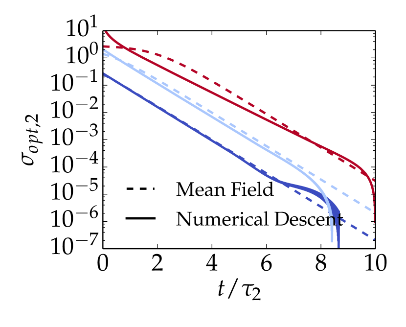
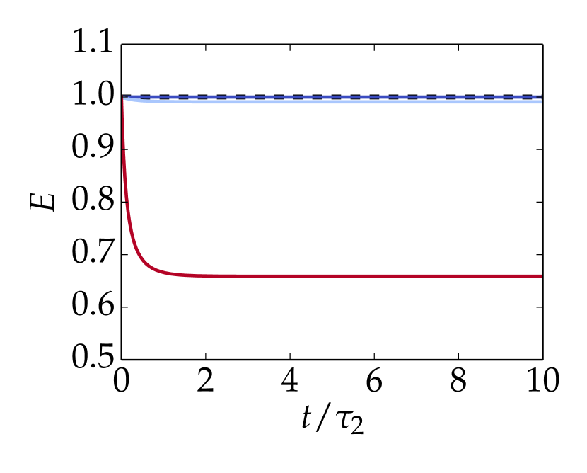
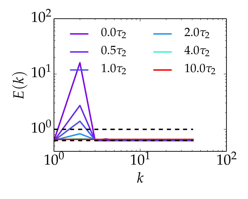
Figure 2: The left panel compares the mean-field (26) and the iterative determination of the optimal control $\sigma_{opt,2}$, that determines the stationary response to a single-mode disturbance of the mode $k=2$ out of $K=41$ active modes, for initial disturbances $b_{2}=\beta/1.1$ ($\bullet$) , $\beta/2$ ($\bullet$) and $\beta/16$ ($\bullet$). The upper right panel shows the time evolution of the total energy as determined by the numerical optimization. The lower right panel shows the corresponding evolution of the normalized energy spectrum $E(k)=\beta/b_{k}$ from the highest initial perturbation $b_{2}=\beta/16$ towards a “wrong” equipartition state. The descent optimizes the cost between $0$ and $t=10\tau_{2}$, the initial total energy is $1$, and convergence is declared when the amplitude of the cost gradient becomes smaller than $g_{tol}=10^{-6}$.

3.4 Constrained minimization and Augmented Lagrangian formalism.

Several strategies can be used to tie the final equipartition state to the initial value of the ensemble energy, either at the level of the trial densities or at the level of the optimization problem. We decide for the latter option. We redefine the optimal control as the solution to the following constrained minimization problem, where the statistical conservation of the energy is imposed by a constraint $\mathcal{C}({\bf b},{\boldsymbol{\sigma}})$ that depends on the state and the control :

$$\underset{[{\boldsymbol{\sigma}}]}{\inf}\int_{0}^{t}\text{d}s\;L_{lof}\left({\bf b}(s),{\boldsymbol{\sigma}}(s)\right)\text{~{}subject to ~{}}\begin{cases}&{\bf b}[t=0]={\bf b}_{0},\\ &\dot{\bf b}={\boldsymbol{\phi}}({\bf b},{\boldsymbol{\sigma}})\text{~{}with ~{}}\phi_{l}({\bf b},{\boldsymbol{\sigma}})=b_{l}\sigma_{l},\\ &\text{and~{}}0=\dot{E}=\mathcal{C}({\bf b},{\boldsymbol{\sigma}})=-\sum_{l=1}^{K}\sigma_{l}/b_{l}.\end{cases}$$ (27)

Robust numerical algorithms are documented to solve such globally constrained optimization problems, one example being the augmented Lagrangian method (see [31, Chapters 12 and 17] and references therein). To enforce energy conservation, we use a time-dependent Lagrange multuplier $\lambda(s)$ and a scalar penalty factor $\mu$ in the augmented objective function :

$$\begin{split}&\tilde{\mathcal{J}}_{\lambda,\mu}[[{\boldsymbol{\sigma}}],t]=\int_{0}^{t}\text{d}s\;\left(\dot{\bf b}(s)\cdot{\boldsymbol{\pi}}(s)-\mathcal{H}_{P,\lambda,\mu}({\bf b}(s),{\boldsymbol{\pi}}(s),{\boldsymbol{\sigma}}(s))\right),\\ &\text{where ~{}}\mathcal{H}_{P,\lambda,\mu}={\boldsymbol{\phi}}\cdot{\boldsymbol{\pi}}-L_{lof}({\bf b},{\boldsymbol{\sigma}})+\lambda\mathcal{C}({\bf b},{\boldsymbol{\sigma}})-\dfrac{1}{2\mu}\mathcal{C}^{2}({\bf b},{\boldsymbol{\sigma}})\end{split}$$ (28)

now defines the augmented Hamilton-Pontryagin function. The descent algorithm and the updating scheme for $\lambda$ and $\mu$ are described in B (Algorithm 2). The convergence is declared when both the gradient of the objective cost and the constraint norm become smaller than pre-defined tresholds, say $g_{tol}$ and $c_{tol}$.

Figure 3 illustrates the algorithm’s consistency for the single-mode disturbance scenario, and shows the convergence towards the correct equipartition state. The departure from the mean-field prediction for the largest perturbations is due to the mean-field assumption that all the undisturbed modes remain exactly in equipartition.

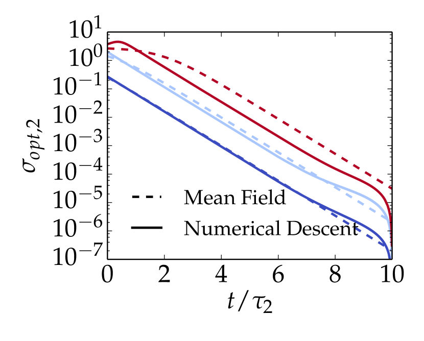
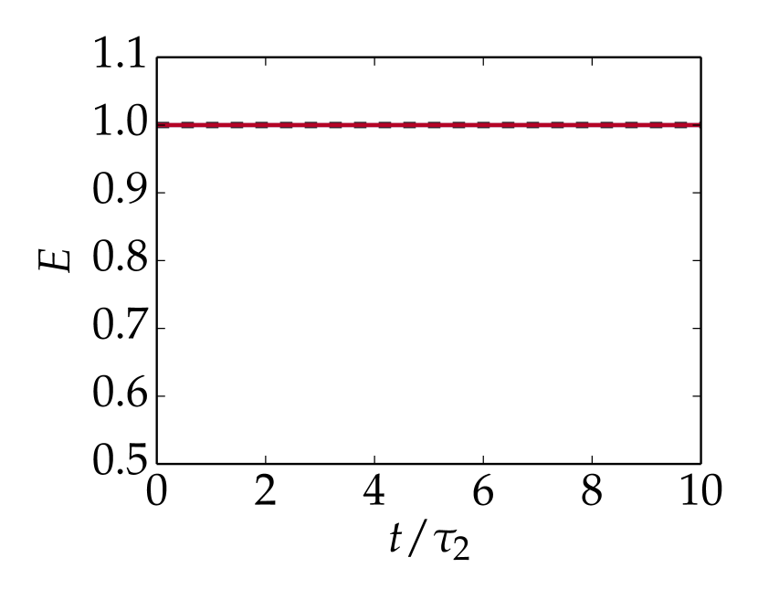
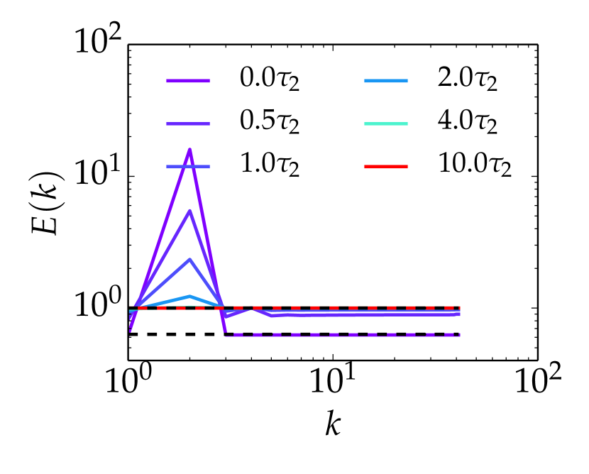
Figure 3: Same as Figure 2, but the iterative determination now incorporates the conservation of the energy through the augmented Lagrangian method. The lower right panel now shows the stationary evolution of the the normalized energy spectrum $E(k)=\beta/b_{k}$ from the highest initial perturbation $b_{2}=\beta/16$ towards the correct equipartition state. Convergence is declared when the amplitude of the augmented cost gradient becomes smaller than $g_{tol}=10^{-6}$, and the constraint norm is smaller than $c_{tol}=10^{-4}$.

3.5 The optimal response algorithm.

The optimal response algorithm (Algorithm 1) sequentially pieces together the augmented Lagrangian method and the non-linear conjugate gradient descent to compute the optimal response with the desired accuracies $g_{tol}$ and $c_{tol}$ up to time $t$. The process essentially consists in first approximating the envelope with loose convergence criteria, and then in refining the envelope up to the prescribed accuracy. The second step can be done in parallel.

Algorithm 1 The optimal response algorithm

1:  Set a sequence $T_{0}=0<T_{1}<\dots<T_{k}=t$ of final times. The $T_{i}$’s need not be linearly spaced.

2:  For each $T_{i}$, compute the shadow response $\tilde{b}(\cdot|T_{i})$ using the augmented Lagrangian algorithm up to relaxed convergence criterion $g_{tol}^{\prime}>g_{tol}$ and $c_{tol}^{\prime}>c_{tol}$ . As a first guess for the initial values of both the control and the augmentation weights, take the converged values corresponding to time $T_{i-1}$.

3:  For each $T_{i}$, use the previously “loosely” converged controls and augmentation weights to initialize the augmented-descent algorithm and reach the prescribed accuracies $g_{tol}$ and $c_{tol}$.

4:  Interpolate the final time values of the final states to obtain the optimal response.

4 Numerical experiments.

We now use the optimal response algorithm to examine the predictive skill of the optimal response framework for Burgers dynamics, and compare it to both direct numerical simulations (DNS) and F/D type predictions. More specifically, we study the non-equilibrium response to two specific types of perturbations (i) a “single-mode disturbance” away from equipartition, and (ii) a “many-mode disturbance”. For both scenarios, we find that the optimal and the F/D predictions have a comparable range of relevance.

4.1 Single-Mode vs Many-Mode disturbances.

In the single-mode perturbation scenario, a single mode $k$ carries most of the disturbance away from equipartition. This is the case previously described by Equation (30), which we here define in terms of the disturbance amplitude $\Delta_{0}$ as :

$${\bf b}_{0,l}=\beta/\Delta_{0}\text{~{}if $l=k$, and~{}}\dfrac{K-1}{K-\Delta_{0}}\beta\text{~{}~{}otherwise}.$$ (29)

In the many-mode perturbation scenario, the $k-1$ modes graver than $k$ carry the same amount of disturbance away from equipartition. The initial ensemble is then taken as :

$${\bf b}_{0,l}=\beta/\Delta_{0}\text{~{}if $l<k$, and~{}}\dfrac{K-k+1}{K-k\Delta_{0}}\beta\text{~{}~{}otherwise}.$$ (30)

In both cases, the (average) equipartition energy contained in each shell is $E_{eq}=1/\beta$, so that the total energy is $E=K/\beta$. In our numerics, we systematically set the total energy to $1$. The amplitude $\Delta_{0}$ represents the excess energy in the disturbed modes $k$ : at initial time, they each have the same energy $E_{k}=\langle|v_{k}|^{2}\rangle=\Delta_{0}E_{eq}$.

4.2 Computing Averages.

For both scenarios (single-mode and many-mode disturbances), we estimate the relaxation of the energy spectrum in three different ways : using DNS to estimate the true ensemble averages, using the F/D estimate (7), and using the optimal response algorithm for the optimal estimate (19).

DNS.

True non-equilibrium averages are estimated by making ensemble averages from individual realizations of the relaxation, computed with DNS. The TBH dynamics (1) is integrated in time with a standard $4^{th}$-order Runge- Kutta algorithm. The non-linear terms are estimated with a pseudo-spectral method, that uses the 2/3-rule dealiasing [32]. The results that we report here correspond to DNS with spatial resolutions of $N=128$ and $N=512$ grid points. The corresponding cutoffs in Fourier space are then exactly $K=42$ and $K=170$. The time-steps are taken as $\delta t=3.9\times 10^{-3}$ and $9.8\times 10^{-4}$, and guarantee an accurate conservation of the energy. Averages are taken over 20,000 realizations.

F/D estimate.

To estimate the energy spectrum relaxation with the F/D relations, we need to determine numerically the response functions $R_{k}^{l}$. This is done by performing averages of DNS realizations sampled from equipartition, with parameters similar to those defined in the previous paragraph. To improve the statistical accuracy, we use the symmetric part of the correlation functions $\langle|v_{k}(t)|^{2}|v_{l}(0)|^{2}\rangle_{DNS}$ to determine the response function. This is justified, provided that the underlying statistics are indeed stationary. Figure 4 shows the short time-behavior of the so-determined response functions for a $512$ resolution.

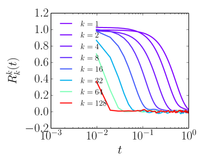
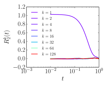
Figure 4: Short-time behavior of the diagonal elements (left) and the two-mode correlation $(2,k)$ (right) of the response function, computed by averaging over 20,000 realizations of 512-resolved DNS.

Optimal Response.

The optimal estimates of the non-equilibrium averages are obtained from the optimal response algorithm. The numerical precisions are set to $g_{tol}=10^{-6}$ and $c_{tol}=10^{-4}$. The time-steps are $\delta t^{\prime}=1.2\times 10^{-2}$ for the 128 case, and $\delta t^{\prime}=7.8\times 10^{-4}$ for the 512 case. The final times $T$ at which the shadow responses are computed are taken to be logarithmically spaced between $T_{1}=4\delta t$ and $T_{f}=5.$ For the 128 case, we refine the short-time computation of the optimal enveloppe by determining additional shadow responses between $T=4\delta t^{\prime}$ and $T=0.1$. For those additional points, we use the value $\delta t^{\prime}$ for the time-steps of the shadow responses.

4.3 Results.

Single-mode disturbances.

We show the responses to single-mode perturbations for both low and high modes, namely $k=1,2,4,8,16$ and $32$, and using $\Delta_{0}=1.1,2,4$ and $8$ for the amplitude of the initial disturbances. The numerical outcomes are summarized in Figures (5) and (6), which display the decay towards equipartition of the three estimates for the non-equilibrium averages of the disturbed energy at mode $k$. We use as the natural time-scale the mean-field time $\tau_{k}=k^{-1}E^{-1/2}$ previously encountered in Equation (26).

Figure 5: The figures show the decay of the most perturbed mode $k$ back to equipartition after single-mode disturbance, for $\Delta_{0}=1.1,2,4,8$ (from left to right and top to bottom). The energies are normalized to their equipartition value $1/\beta$. The DNS resolution is $N=128$. The colors code the wavenumber of the disturbed mode. The symbols code the averages : DNS (solid line), F/D (diamonds) and optimal (circles). The insets show the corresponding energy spectra, which is perturbed at initial time and undistinguishable from equipartition at final time.

Figure 6: Same as Figure 5, for a DNS resolution $N=512$. Only the respones to the single-mode disturbances $\Delta_{0}=2$ (left) and $\Delta_{0}=4$ (right).

For the smallest perturbations $\Delta_{0}=1.1$ and $2$, the three averages (true, F/D and optimal) are indistinguishable from one another. This is visible for both the $N=128$ and $N=512$ cases. The collapse is perfect in all of the three stages of the energy relaxation : the initial stage up to $t\approx 0.2\tau_{k}$ where the energy remains essentially constant, the intermediate relaxation stage $0.2\tau_{k}\lesssim t\lesssim\tau_{k}$ and the final equilibrium stage after $\tau_{k}$. Discrepancies start to be noticeable for the two highest initial disturbances. The optimal responses capture the natural time scaling and the collapse of the relaxation profiles when the time is normalized by $\tau_{k}$. However, the initial stage of zero dissipation of energy ends too soon, and the intermediate stage is slightly longer than in the DNS. This feature is particularly visible for the 512 runs (see Figure 6, right panel).

Many-mode disturbances.

The same qualitative features are observed for the many-mode disturbance scenario, as displayed on Figure 7. For the small amplitude perturbations $\Delta_{0}=2$ displayed on the top panel, the agreement between the three types of averages is excellent, whether the number of disturbed modes is small or large. Discrepancies are apparent for larger initial perturbations (bottom panel), for which the “undisturbed” higher modes are initially far away from their thermalized values. For the case where only the first three modes are disturbed, we observe as in the single-mode case that the optimal response has a good qualitative behavior but starts to decay too fast compared to DNS. In that case, the F/D estimate apparently gives a correct prediction of the DNS averages. When a significant number of modes are taken away from equipartition, however, both the F/D and the optimal responses break down. It is interesting to observe that in that case, the optimal responses do not collapse any longer with the time scale $\tau_{k}$, and nor do the DNS. The qualitative behavior of the optimal response is surprising. It predicts an energy transfer from the low modes to the high modes during the initial stage, resulting in a too fast decay of the high modes and a too slow decay for the low modes, characterized by an initial bump in the energy profile.

Figure 7: The figures show the decay of the $k-1$ most perturbed modes back to equipartition after a many-mode disturbance, for $\Delta_{0}=2$ (top) and $8$ (bottom) and $k=2$ (left) and $16$ (right) . The energies are normalized to their equipartition value $1/\beta$. The DNS resolution is $N=512$. The colors code the wavenumber of the disturbed modes. The symbols code the averages : DNS (solid line), F/D (diamonds) and optimal (circles). The insets show the corresponding energy spectra, which is perturbed at initial time and undistinguishable from equipartition at final time.

We therefore conclude that the optimal response is accurate for perturbations of moderate amplitudes, in which case it displays a mean-field behavior and is indistinguishable from the true DNS. For higher perturbations, the skill of the optimal response theory breaks down, as seemingly non-physical inverse energy transfers are predicted. It appears that the range of applicability of the optimal responses is slightly more restricted than that of the F/D approach.

5 Conclusion.

In this paper we have shown that the best-fit dynamical optimization recently exposed in a series of papers provides a fully predictive theory, as one can use standard optimization algorithms to determine the optimal response. The optimal response algorithm described in Section 3 achieves such a task. We were able to test the skill of the best-fit theory per se, without relying to further approximations (mean-field, perturbation expansions) to solve the underlying Hamilton-Jacobi equation. In the near-equilibrium regime, the optimal estimates are consistent with DNS, and share a similar range of applicability as linear F/D estimates – although perhaps slightly more restricted. In contrast to the latter, we emphasize that the optimal responses are computed self-consistenly and independently from DNS. This makes the optimal response an approximate but fully predictive theory.

From a more conceptual point of view, the use of the optimal response algorithm beyond the mean-field regime revealed a flaw of the original dynamical optimization, namely that the optimal responses fail to conserve energy in general. The defect is an undesired consequence of the degeneracy of the lack-of-fit potential, but can be easily fixed by imposing energy conservation in the optimization principle. Perhaps, the origin of the degeneracy relates to the single-time nature of the theory.

We have restricted our exposition to simple quasi-Gibbsian trial densities. In principle, patience is the only virtue required to compute the lack-of-fit Hamiltonian associated to more accurate trial densities. The optimal response algorithm provides a a systematic way to compute the associated best-fit response and can in principle be used to investigate more refined Ansätze that include non-Gibbsian parts. We hope that those could prove efficient to model the decay of far-from-equilibrium disturbances. Let us however observe that the algorithm performs a multi-layer optimization descent on a high dimensional space. In the quasi-Gibbsian case, the underlying assumption is that the many-mode correlations need not be modeled to give accurate estimates, so that the number of variables in the optimization problem scales linearly with the size of the problem. This hypothesis will break down further away from equilibrium. In order to optimize over many-mode correlations, an appropriate modeling effort will therefore be required at the level of the trial densities themselves, in order to make the numerical optimization computationally tractable.

Appendix A The mean-field approximation to the lack-of-fit Hamiltonian

The optimal response for a single-mode perturbation $k$ away from equipartition can be obtained via a mean-field argument, that consists in putting $b_{l}(t)=\beta$ for the non-perturbed modes in the lack-of-fit Hamiltonian (17) The resulting reduced lack-of-fit Hamiltonian now depends on a single pair of conjugate variables $(b_{k},\pi_{k})$, which we write suggestively as follows :

$$\begin{split}&\mathcal{H}_{lof}(b_{k},\pi_{k})=\dfrac{\pi_{k}^{2}b_{k}^{2}}{2}-\mathcal{U}[b_{k}],\text{~{}with~{}~{}}\mathcal{U}[b_{k}]=C_{1}\left(\dfrac{1}{b_{k}}-\dfrac{1}{\beta}\right)+C_{2}\left(\dfrac{b_{k}}{\beta^{2}}-\dfrac{1}{\beta}\right)\\ &\text{and}~{}C_{1}=k^{2}K\left(1-\dfrac{k+7}{2K}\right)~{},~{}C_{2}=k^{2}K\left(1-\dfrac{k+3}{2K}\right).\end{split}$$ (31)

For $k/K\ll 1$ , which corresponds to a large-scale perturbation, we can recast the lack-of-fit potential as

$$\begin{split}&\mathcal{U}[b_{k}]=\dfrac{\beta}{\tau_{k}^{2}b_{k}}\left(1-\dfrac{b_{k}}{\beta}\right)^{2}\text{~{}with~{}}\tau_{k}=k^{-1}E^{-1/2}\text{~{}and $E$ the total energy.}\\ \end{split}$$ (32)

The stationary shadow path is then defined by the equality $\mathcal{H}_{lof}(b_{k},\pi_{k})=\mathcal{H}_{lof}(\beta,0)=0$, which leads directly to (26). In the mean-field approximation, the non-perturbed modes $l\neq k$ act as a thermal bath that sinks the excess energy induced by the initial perturbation. As such, the total energy is not conserved.

Appendix B Discrete formulation of the optimal response algorithm.

In this appendix, we expose the details of the optimal response algorithm. The practical implementation relies on a discrete approximation, which is performed directly at the level of the objective cost. Standard algorithms can then be used to solve the discrete optimization problems.

B.1 Discretizing the optimization problem.

In this subsection, we define a discrete version of the minimization problem (27). We define a discrete counterpart to the augmented objective cost, that involve a discrete augmented lack-of-fit Pontryagin Hamiltonian.

Discrete Notations.

We write $t$ the final time involved in (27). We define the time step $h=t/{N_{t}}$, and discretize the time interval $[0;t[$ into the ${N_{t}}$ time intervals $[t_{i};t_{i+1}[$, delimited by the discrete times $t_{i}=ih$. We write ${\bf s}_{i}={\bf s}(t_{i})$, ${\boldsymbol{\pi}}_{i}={\boldsymbol{\pi}}(t_{i})$ and ${\boldsymbol{\sigma}}_{i}={\boldsymbol{\sigma}}(t_{i})$, the values of the state, co-state and control variables at the discrete times $t_{i}$. The notation ${\bf s}$, without subscript, denotes ${\bf s}=({\bf s}_{i})_{0\leq i\leq{N_{t}}}$. Recall that the $({\bf s}_{i})$’s are $\mathbb{R}^{K}$ vectors, so that for example $s_{i,l}$ denotes the $l^{th}$ component of the state variable at time $t_{i}$, and that we use the notation ${\bf a}_{i}\cdot{\bf b}_{i}=\sum_{l=1}^{K}a_{i,l}b_{i,l}$. Note that we here prefer to use the symbol ${\bf s}$ to denote the state variable, so that the latter is not necessarily taken to be the inverse temperature ${\bf b}$, as was the case in Section (3).

We use the trapezoidal rule to estimate the time integrals. The discrete counterpart to the minimization problem (27) is then

$$\underset{{\boldsymbol{\sigma}}}{\inf}~{}h\sum_{i=0}^{{N_{t}}-1}\dfrac{L_{i}+L_{i+1}}{2}\text{~{}subject to ~{}}\begin{cases}&{\bf s}[t=0]={\bf s}_{0},\\ &{\bf s}_{i+1}-{\bf s}_{i}=h\,{\boldsymbol{\phi}}({\bf s}_{i},{\boldsymbol{\sigma}}_{i})=h{\boldsymbol{\phi}}_{i},\\ &\text{and~{}}0=\mathcal{C}({\bf s}_{i},{\boldsymbol{\sigma}}_{i})=\mathcal{C}_{i}.\end{cases}$$ (33)

where we use the short-hand notation $L_{i}=L_{lof}\left({\bf s}_{i},{\boldsymbol{\sigma}}_{i}\right)$. $\phi$ and $\mathcal{C}$ are prescribed functions of their arguments. If ${\bf s}$ is the inverse temperature vector, the state equation reads $\phi_{l}({\bf s}_{i},{\boldsymbol{\sigma}}_{i})=s_{i,l}\sigma_{i,l}$ and $\mathcal{C}({\bf s}_{i},{\boldsymbol{\sigma}}_{i})=-{\boldsymbol{\sigma}}_{i}\cdot{\bf s}_{i}^{-1}$. In practice, a convenient choice is to take the state as the neg-entropy vector, namely ${\bf s}=\log{\bf b}/\beta$. This choice guarantees that the algorithm will not optimize over non-realizable negative inverse temperature vectors. if ${\bf s}$ is the neg-entropy, the state equation is $\phi_{l}({\bf s}_{i},{\boldsymbol{\sigma}}_{i})=\sigma_{i,l}$ and the energy dissipation constraint reads $\mathcal{C}({\bf s}_{i},{\boldsymbol{\sigma}}_{i})={\boldsymbol{\sigma}}_{i}\cdot e^{-{\bf s}_{i}}$.

The Discrete augmented cost and its gradient.

To solve the optimization problem (33), we define the discrete augmented cost as a counterpart to (28) :

$$\begin{split}&\mathcal{J}_{\lambda,\mu}[{\boldsymbol{\sigma}}]=\sum_{i=0}^{{N_{t}}-1}\dfrac{{\boldsymbol{\pi}}_{i}+{\boldsymbol{\pi}}_{i+1}}{2}\cdot\left({\bf s}_{i+1}-{\bf s}_{i}\right)-h\dfrac{H_{i}+H_{i+1}}{2},\\ &\text{where~{}}H_{i}={\boldsymbol{\pi}}_{i}\cdot{\boldsymbol{\phi}}_{i}-L_{i}+\lambda_{i}\mathcal{C}_{i}-\dfrac{1}{2\mu}\mathcal{C}_{i}^{2}=\mathcal{H}_{P,\lambda_{i},\mu}({\bf s}_{i},{\boldsymbol{\pi}}_{i},{\boldsymbol{\sigma}}_{i}).\end{split}$$ (34)

denotes the discrete counterpart to the augmented Hamilton-Pontryagin function. For the notation (34) to be self-consistent, and for the cost to be a function of the control only, the state and the co-state need to be enslaved to it. The good prescription is to define the states and the co-states recursively as follows :

$$\begin{split}{\bf s}_{0}={\bf s}[t=0],~{}{\bf s}_{1}={\bf s}_{0}+h\nabla_{{\boldsymbol{\pi}}_{0}}H_{0}\text{~{}~{}and~{}~{}}{\bf s}_{i}={\bf s}_{i-1}+2h\nabla_{{\boldsymbol{\pi}}_{i}}H_{i}\text{~{}~{}($i>1$)};\\ \pi_{N_{t}}=0,~{}{\boldsymbol{\pi}}_{{N_{t}}-1}=h\nabla_{{\bf s}_{N_{t}}}H_{N_{t}}\text{~{}~{}and~{}~{}}{\boldsymbol{\pi}}_{i-1}={\boldsymbol{\pi}}_{i+1}+2h\nabla_{{\bf s}_{i}}H_{i}\text{~{}~{}($i<{N_{t}}-1$)}.\end{split}$$ (35)

Those two equations are the discrete counterpart to Equation (23). The gradient of the augmented cost with respect to the ${N_{t}}\times K$ control variables $\sigma_{i,l}$ is then obtained as

$$\nabla_{\boldsymbol{\sigma}}\mathcal{J}_{\lambda,\mu}=\left(\dfrac{\partial\mathcal{J}_{\lambda,\mu}}{\partial\sigma_{i,l}}\right)_{\begin{subarray}{c}0\leq i\leq{N_{t}}\\ 1\leq l\leq K\end{subarray}}\text{with }\dfrac{\partial\mathcal{J}_{\lambda,\mu}}{\partial\sigma_{i,l}}=\begin{cases}&-h\dfrac{\partial\mathcal{H}_{i}}{\partial\sigma_{i,l}}\text{~{}~{}if $0<i<{N_{t}}$},\\ &-\dfrac{h}{2}\dfrac{\partial\mathcal{H}_{i}}{\partial\sigma_{i,l}}\text{~{}~{}if $i=0$ or $i={N_{t}}$}.\\ \end{cases}$$ (36)

To see that the prescription (35) is correct and leads to the gradient (36), it suffices to obtain the infinitesimal variation of the cost with respect to the state, co-state and control variables as :

$$\begin{split}2\delta\mathcal{J}=&\sum_{i=1}^{{N_{t}}-1}\delta{\boldsymbol{\pi}}_{i}\cdot\left({\bf s}_{i+1}-{\bf s}_{i-1}-2h\nabla_{{\boldsymbol{\pi}}_{i}}H_{i}\right)+\delta{\bf s}_{i}\cdot\left({\boldsymbol{\pi}}_{i-1}-{\boldsymbol{\pi}}_{i+1}-2h\nabla_{{\bf s}_{i}}H_{i}\right)\\ &+\delta{\boldsymbol{\pi}}_{N_{t}}\cdot\left({\bf s}_{{N_{t}}}-{\bf s}_{{N_{t}}-1}-h\nabla_{{\boldsymbol{\pi}}_{N_{t}}}H_{N_{t}}\right)+\delta{\boldsymbol{\pi}}_{0}\cdot\left({\bf s}_{1}-{\bf s}_{0}-h\nabla_{{\boldsymbol{\pi}}_{0}}H_{0}\right)\\ &+\delta{\bf s}_{N_{t}}\cdot\left({\boldsymbol{\pi}}_{{N_{t}}}+{\boldsymbol{\pi}}_{{N_{t}}-1}-h\nabla_{{\bf s}_{N_{t}}}H_{N_{t}}\right)+\delta{\bf s}_{0}\cdot\left(-{\boldsymbol{\pi}}_{0}-{\boldsymbol{\pi}}_{1}-h\nabla_{{\bf s}_{0}}H_{0}\right)\\ &-2\sum_{i=1}^{{N_{t}}-1}h\delta{\boldsymbol{\sigma}}_{i}\cdot\nabla_{{\boldsymbol{\sigma}}_{i}}H_{i}-h\delta{\boldsymbol{\sigma}}_{0}\cdot\nabla_{{\boldsymbol{\sigma}}_{0}}H_{0}-h\delta{\boldsymbol{\sigma}}_{N_{t}}\cdot\nabla_{{\boldsymbol{\sigma}}_{N_{t}}}H_{N_{t}}.\end{split}$$

With the prescription (35), the first three lines of the previous expression vanish. The last line leads directly to (36).

Norms.

To control the convergence of the numerics and define stopping criteria, we define norms for both the cost gradient (36) and the constraint. We use for the gradient :

$$||\nabla_{\sigma}\mathcal{J}||=\dfrac{1}{K}\left(\sum_{i=0}^{{N_{t}}}\sum_{l=1}^{K}\left(\dfrac{\partial\mathcal{J}_{\lambda,\mu}}{\partial\sigma_{i,l}}\right)^{2}\right)^{1/2}$$ (37)

As for the constraint satisfiability, that determines how well the energy is conserved :

$$||\mathcal{C}||=\sup_{0\leq i\leq{N_{t}}}|\mathcal{C}_{i}|.$$ (38)

B.2 Implementation of the optimal response algorithm.

Augmented Lagrangian descent.

Algorithm 2 describes the augmented Lagrangian descent method involved in the optimal response algorithm (3.5). As previously explained, the augmented Lagrangian method provides a strategy to determine iteratively the Lagrange multiplier $\lambda$ and the scalar penalty factor $\mu$, so that the norms of both the constraint and the cost gradient utlimately become lower than some prescribed convergence levels $c_{tol}$ and $g_{tol}$. We use a simplified version of the LANCELOT method of multipliers described in [31] (Chapter 17, algorithm 17.4). In a nutshell, it consists in decreasing $\mu$ when the constraint is not sufficiently satisfied and updating $\lambda$ otherwise, so that the latter mimics the behavior of Lagrange multiplier.

Algorithm 2 Augmented descent with the LANCELOT method of multipliers

1:  $\mu\leftarrow\mu^{(0)}$ {Initialize the weigths}

2:  $\lambda\leftarrow\lambda^{(0)}$

3:  $\tilde{g}_{tol}\leftarrow\max\,\left\{\mu,\,g_{tol}\right\}$ {Initialize loosened tolerances}

4:  $\tilde{c}_{tol}\leftarrow\max\,\left\{\mu^{{\alpha_{2}}},\,c_{tol}\right\}$

5:  while $||\nabla_{\boldsymbol{\sigma}}J||>g_{tol}$ or $||\mathcal{C}||>c_{tol}$ do

6:     Determine ${\boldsymbol{\sigma}}_{\lambda,\mu}^{\star}=\arg\inf J_{\lambda,\mu}$ with precision $\tilde{g}_{tol}$ {Unconstrained Descent}

7:     if $||\mathcal{C}||<c_{tol}$  then

8:        $\lambda_{i}\leftarrow\lambda_{i}-\dfrac{\mathcal{C}_{i}}{\mu}$ {Update $\lambda$}

9:        $\tilde{c}_{tol}\leftarrow\max\left\{\tilde{c}_{tol}\mu^{\alpha_{1}}\,,\,c_{tol}\right\}$ {Tighten tolerances}

10:        $\tilde{g}_{tol}\leftarrow\max\left\{\tilde{g}_{tol}\mu\,,\,g_{tol}\right\}$

11:     else

12:        $\mu\leftarrow\tau\mu$ with $\tau=\min\left\{0.2,\,\sqrt{\mu}\right\}$ {Update $\mu$}

13:        $\tilde{c}_{tol}\leftarrow\max\left\{\tilde{c}_{tol}\mu^{\alpha_{2}},\,c_{tol}\right\}$ {Tighten tolerances}

14:        $\tilde{g}_{tol}\leftarrow\max\left\{\mu,g_{tol}\right\}$

15:     end if

16:  end while

17:  return  ${\boldsymbol{\sigma}}_{\lambda,\mu}^{\star}$ {Return the optimal control}

For all of our numerics, we used the empirical values ${\alpha_{1}}=0.9$ and ${\alpha_{2}}=0.1$ to control the tightening of the tolerances. If no initial guess was provided, we used $\mu^{(0)}=0.1$ and $\lambda^{(0)}=0$.

Unconstrained descent.

The success of the augmented descent method is dependent upon having an efficient unconstrained descent solver, to determine the minimum of the augmented cost $J_{\lambda,\mu}$ up to the desired tolerances $\tilde{g}_{tol}$ and $\tilde{c}_{tol}$. We found that the non-linear conjugate gradient method with Polak-Ribière⁺ updates (see Chapter 5 and Formula (5.43) of [31]) is here suited for the task. This is a standard and well-documented method, which we describe in Algorithm (3) for the sake of clarity.

Algorithm 3 The non-linear conjugate gradient descent

1:  ${\boldsymbol{\sigma}}\leftarrow{\boldsymbol{\sigma}}_{\lambda,\mu}^{(0)}$ {Initial guess}

2:  $J\leftarrow\mathcal{J}_{\lambda,\mu}({\boldsymbol{\sigma}},t)$ {From Equations (35) and (34)}

3:  $\nabla J\leftarrow\nabla_{\boldsymbol{\sigma}}\mathcal{J}_{\lambda,\mu}({\boldsymbol{\sigma}})$ {Using Equation (36)}

4:  ${\bf p}\leftarrow-\nabla J$ {Initial guess for the descent direction}

5:  while $||\nabla J||>g_{tol}$ do

6:     Find $\alpha$ such that ${\boldsymbol{\sigma}}+\alpha{\bf p}$ satisfies the strong Wolfe Conditions, namely

$$J({\boldsymbol{\sigma}}+\alpha{\bf p})\leq J+c_{1}\alpha\nabla J\cdot{\bf p}\text{~{}and~{} }\nabla_{\boldsymbol{\sigma}}\mathcal{J}_{\lambda,\mu}({\boldsymbol{\sigma}}+\alpha{\bf p})\cdot{\bf p}\geq c_{2}\nabla J\cdot{\bf p}.$$ (39)

7:     ${\boldsymbol{\sigma}}\leftarrow{\boldsymbol{\sigma}}+\alpha{\bf p}$.

8:     $J\leftarrow\mathcal{J}_{\lambda,\mu}({\boldsymbol{\sigma}},t)$

9:     $\nabla J^{\prime}\leftarrow\nabla J$ and $\nabla J\leftarrow\nabla_{\boldsymbol{\sigma}}\mathcal{J}_{\lambda,\mu}({\boldsymbol{\sigma}},t)$

10:     ${\bf p}\leftarrow\gamma{\bf p}-\nabla J$ with $\gamma=\max\left\{\gamma^{PR},0\right\}$ and $\gamma^{PR}=\dfrac{\nabla J\cdot\left(\nabla J-\nabla J^{\prime}\right)}{\nabla J^{\prime}\cdot\nabla J^{\prime}}$

11:  end while

12:  return  ${\boldsymbol{\sigma}}$

The non-linear conjugate gradient descent uses yet another layer of optimization. As apparent on on lines 6 and 7 of Algorithm (3), it requires to perform a unidimensional optimization, in order to find a scalar $\alpha$ that verifies the so-called strong Wolfe conditions (39), for prescribed parameters $c_{1}$ and $c_{2}$. Fortunately, this kind of optimization is very standard, and a suited value for the scalar $\alpha$ can be found using the default line-search algorithms implemented in most programming languages. In this work, we used the Python programming language (Python Software Foundation, https://www.python.org/). The line-search function available from the scipy.optimize package implements Algorithm 3.2 of [31, Chapter 3 ]) and performs a unidimensional optimization thats finds a scalar $\alpha$ that verifies the strong Wolfe conditions. In our numerics, we have used $c_{1}=10^{-3}$ and $c_{2}=0.5$.

References

References

- [1] Ryogo Kubo, Morikazu Toda, and Natsuki Hashitsume. Statistical physics II: nonequilibrium statistical mechanics, volume 31. Springer Science & Business Media, 2012.
- [2] David Chandler. Introduction to modern statistical mechanics. Introduction to Modern Statistical Mechanics, by David Chandler, pp. 288. Foreword by David Chandler. Oxford University Press, Sep 1987. ISBN-10: 0195042778. ISBN-13: 9780195042771, 1, 1987.
- [3] Hannes Risken. Fokker-planck equation. In The Fokker-Planck Equation, pages 63–95. Springer, 1984.
- [4] Christian Maes. On the second fluctuation- dissipation theorem for nonequilibrium baths. Journal of Statistical Physics, 154(3):705–722, 2014.
- [5] Robert H. Kraichnan. Irreversible Statistical Mechanics of Incompressible Hydromagnetic Turbulence. Phys. Rev., 109(5):1407–1422, 1958.
- [6] Robert H. Kraichnan. Classical Fluctuation-Relaxation Theorem. Phys. Rev., 113(5):1181–1182, 1959.
- [7] L. Biferale, I. Daumont, G. Lacorata, and A. Vulpiani. Fluctuation-response relation in turbulent systems. Phys. Rev. E, 65(1):016302, 2001.
- [8] Robert H. Kraichnan. Lagrangian History Closure Approximation for Turbulence. Physics of Fluids (1958-1988), 8(4):575–598, 1965.
- [9] Robert H. Kraichnan. Lagrangian History Statistical Theory for Burgers’ Equation. Physics of Fluids (1958-1988), 11(2):265–277, 1968.
- [10] Gregory Eyink and Uriel Frisch. Robert H. Kraichnan. In A Voyage Through Turbulence. Cambridge University Press, 2010.
- [11] C. E. Leith. Climate Response and Fluctuation Dissipation. J. Atmos. Sci., 32(10):2022–2026, 1975.
- [12] Thomas L. Bell. Climate Sensitivity from Fluctuation Dissipation: Some Simple Model Tests. J. Atmos. Sci., 37(8):1700–1707, 1980.
- [13] Andrey Gritsun, Grant Branstator, and Andrew Majda. Climate response of linear and quadratic functionals using the fluctuation-dissipation theorem. Journal of the Atmospheric Sciences, 65(9):2824–2841, 2008.
- [14] Andrew J. Majda. Challenges in Climate Science and Contemporary Applied Mathematics. Comm. Pure Appl. Math., 65(7):920–948, 2012.
- [15] Bruce Turkington and Petr Plechac. Best-fit quasi-equilibrium ensembles: a general approach to statistical closure of underresolved Hamiltonian dynamics. arXiv:1010.4362 [math-ph], 2010. arXiv: 1010.4362.
- [16] Bruce Turkington. An Optimization Principle for Deriving Nonequilibrium Statistical Models of Hamiltonian Dynamics. J Stat Phys, 152(3):569–597, 2013.
- [17] Richard Kleeman and Bruce E. Turkington. A Nonequilibrium Statistical Model of Spectrally Truncated Burgers-Hopf Dynamics. Commun. Pur. Appl. Math., 67(12):1905–1946, 2014.
- [18] Bruce Turkington, Qian-Yong Chen, and Simon Thalabard. Coarse-graining two-dimensional turbulence via dynamical optimization. Nonlinearity, 29(10):2961, 2016.
- [19] Simon Thalabard and Bruce Turkington. Optimal thermalization in a shell model of homogeneous turbulence. Journal of Physics A: Mathematical and Theoretical, 49(16):165502, 2016.
- [20] Andrew J. Majda and Ilya Timofeyev. Remarkable statistical behavior for truncated Burgers–Hopf dynamics. Proceedings of the National Academy of Sciences, 97(23):12413–12417, 2000.
- [21] Cyril Cichowlas, Pauline Bonaïti, Fabrice Debbasch, and Marc Brachet. Effective dissipation and turbulence in spectrally truncated Euler flows. Physical review letters, 95(26):264502, 2005.
- [22] Giorgio Krstulovic and Marc Brachet. Two-fluid model of the truncated Euler equations. Physica D: Nonlinear Phenomena, 237(14):2015–2019, 2008.
- [23] Debarghya Banerjee and Samriddhi Sankar Ray. Transition from dissipative to conservative dynamics in equations of hydrodynamics. Physical Review E, 90(4):041001, 2014.
- [24] Vishwanath Shukla, Stephan Fauve, and Marc Brachet. Statistical theory of reversals in two-dimensional confined turbulent flows. arXiv preprint arXiv:1607.01038, 2016.
- [25] Rafail V. Abramov, Gregor Kovac ic , and Andrew J. Majda. Hamiltonian structure and statistically relevant conserved quantities for the truncated Burgers-Hopf equation. Comm. Pure Appl. Math., 56(1):1–46, 2003.
- [26] Samriddhi Sankar Ray, Uriel Frisch, Sergei Nazarenko, and Takeshi Matsumoto. Resonance phenomenon for the Galerkin-truncated Burgers and Euler equations. Physical Review E, 84(1):016301, 2011.
- [27] Samriddhi Sankar Ray. Thermalized solutions, statistical mechanics and turbulence: An overview of some recent results. Pramana, 84(3):395–407, 2015.
- [28] G. F. Carnevale, M. Falcioni, S. Isola, R. Purini, and A. Vulpiani. Fluctuation- response relations in systems with chaotic behavior. Physics of Fluids A: Fluid Dynamics (1989-1993), 3(9):2247–2254, 1991.
- [29] G. Boffetta, G. Lacorata, S. Musacchio, and A. Vulpiani. Relaxation of finite perturbations: Beyond the fluctuation-response relation. Chaos: An Interdisciplinary Journal of Nonlinear Science, 13(3):806–811, 2003.
- [30] Arthur E Bryson, Yu-Chi Ho, and George M Siouris. Applied optimal control: Optimization, estimation, and control. IEEE Transactions on Systems, Man, and Cybernetics, 9(6):366–367, 1979.
- [31] Jorge Nocedal and Stephen Wright. Numerical optimization. Springer Science & Business Media, 2006.
- [32] Steven A. Orszag. On the elimination of aliasing in finite-difference schemes by filtering high-wavenumber components. Journal of the Atmospheric sciences, 28(6):1074–1074, 1971.