Efficient Metric Learning
for the Analysis of Motion Data

Abstract

We investigate metric learning in the context of dynamic time warping (DTW), the by far most popular dissimilarity measure used for the comparison and analysis of motion capture data. While metric learning enables a problem-adapted representation of data, the majority of methods has been proposed for vectorial data only. In this contribution, we extend the popular principle offered by the large margin nearest neighbors learner (LMNN) to DTW by treating the resulting component-wise dissimilarity values as features. We demonstrate that this principle greatly enhances the classification accuracy in several benchmarks. Further, we show that recent auxiliary concepts such as metric regularization can be transferred from the vectorial case to component-wise DTW in a similar way. We illustrate that metric regularization constitutes a crucial prerequisite for the interpretation of the resulting relevance profiles.

1 Introduction

Motion capture (Mocap) systems rely on a variety of different principles such as magnetic or mechanical sensors, optical markers, poseable mannequins, dedicated technology for hand or facial expression tracking, and low-cost marker-less technology [2, 3]. Powerful analysis software enables the reconstruction of the underlying skeleton when dealing with human motion [4, 5, 6]. These developments cause an increasingly important role of Mocap in diverse areas such as entertainment, sports, or medical applications. When Mocap information is used in complex systems such as virtual trainers or interactive Mocap databases for medical analysis, intelligent data analysis, and machine learning technology become necessary. Proposed methods range from the independent component analysis (ICA) up to deep learning [7, 8].

Within such systems, distance-based methods are often used for the initial analysis or motion retrieval [9, 10, 11]. Due to its capability of adjusting to different durations, dynamic time warping (DTW) constitutes the by far most popular dissimilarity measure in this context [12, 13, 14].

Like any other dissimilarity measure or metric, the results of DTW crucially rely on the choice of its intrinsic parameters; Crucial metric parameters for DTW and similar measures such as alignment are the parameters which determine how two single sequence entries are compared. This is often referred to as the scoring matrix provided a discrete alphabet is chosen, such as DNA or protein sequences. When it comes to sequence alignment in bioinformatics, lots of effort has been made for its correct choice based on biological insight [15]. Provided such insight is not always available, so-called inverse alignment can help to infer metric parameters from given, optimum alignments [16][17]. In general, no such information is present, rather only weak learning signals such as motion labeling or grouping are available. In such cases, the adaptation of metric parameters can be solved by metric learning within a machine learning framework.

Metric learning constitutes a matured field of research for the standard vectorial setting (data represented by feature vectors), e.g., see  [18, 19, 20, 21]. In these approaches, usually, quadratic forms are inferred from the given auxiliary information. This vectorial metric adaptation does not only provide increased model accuracy, but it also dramatically facilitates model interpretability, and it can lead to additional functionalities such as a direct data visualization [22, 23, 24]. Recently, some researches have focussed on the validity of the interpretation of metric parameters as relevance weights, and it has been shown that there exist problems in particular for high-dimensional or highly correlated data [25, 26]. It is possible to avoid these problems by an efficient form of metric regularization as detailed in the approaches[25, 26].

These developments mainly focus on the context of vectorial data; therefore, they are not applicable to distance-based measures, e.g, in the case of DTW. Recently, a few approaches have been proposed which address metric-parameter learning for complex non-vectorial data, in particular sequences and sequence alignment [27, 18, 28]. While these approaches lead to an increased model accuracy and interpretability, they have the drawback that their training complexity is very costly: typically, these techniques adapt metric parameters within sequence alignment, such that pairwise distances of all data samples have to be recomputed after every metric adaptation step.

In this contribution, we take a different point of view for the sake of a significantly reduced computational load: we rely on a representation of sequential data in terms of pairwise dissimilarity vectors as provided by component-wise DTW. This strategy is similar to the popular treatment of dissimilarity data as ‘features’, which is detailed in the monograph [29]. This mathematical formulation enables us to transfer the powerful large margin nearest neighbors (LMNN) metric learner [21] to a metric adaptation for DTW, which is able to adjust the relevance of single joints and their correlations in the Mocap data according to a given specific classification task. Further, we demonstrate that a recent metric regularization framework can be transferred to Mocap DTW results based on the same principle, this way guaranteeing a valid interpretation of the resulting relevance profiles. We demonstrate the efficiency and effectiveness of the proposed methodology for different benchmark datasets.

This contribution is structured as follows: first, we introduce LMNN and its transfer to component-wise DTW, dubbed DTW-LMNN. Afterward, we discuss how the resulting metric can be regularized to avoid its dependency on random effects caused by correlations in the observed data. Finally, we demonstrate the suitability of the proposed methodology in a couple of benchmark Mocap data, where we demonstrate the increased classification accuracy of DTW-LMNN in comparison to alternatives. Finally, we demonstrate the increased interpretability and robustness of the results when metric regularization takes place.

2 Dissimilarity based metric learning

In this section, we review the LMNN algorithm and the DTW distance computation. Then we introduce the proposed algorithm to use the DTW metric along with metric learning optimization, and we discuss how to regularise the resulting dissimilarities to diminish random effects caused by data correlations. Note that DTW is not a metric since the triangle inequality does not hold, rather it is a pairwise symmetric distance function, which can serve as a data dissimilarity measure. Nevertheless, we carelessly refer to DTW as a metric in some places, although strong metric properties do not apply.

2.1 Large margin nearest neighbors metric learning

LMNN is a metric learning algorithm which learns a quadratic form from given labeled data $(\vec{x}^{i},y_{i})\in\mathbb{R}^{n}\times\{1,\ldots,c\}$, $i=1,\ldots,m$, $c=$ number of classes, to improve the classification accuracy of the well-known $k$-nearest neighbors (KNN) method. As a distance-based approach, the accuracy of KNN fundamentally relies on its underlying distance measure which defines the $k$ nearest neighbors of a given data point. LMNN tries to robustly adjust this neighborhood structure by learning a parameterized form

$${\cal D}(\vec{x}^{i},\vec{x}^{j})=(\mathbf{L}(\vec{x}^{i}-\vec{x}^{j}))^{2}=(\vec{x}^{i}-\vec{x}^{j})^{\top}\mathbf{L}^{\top}\mathbf{L}(\vec{x}^{i}-\vec{x}^{j})$$ (1)

with adjustable linear transformation matrix $\mathbf{L}$ which induces a quadratic form characterized by $\mathbf{M}:=\mathbf{L}^{\top}\mathbf{L}$. The objective function of LMNN is based on a fixed $k$-neighborhood structure characterized by $\eta_{ij}\in\{0,1\}$ where $\eta_{ij}=1$ iff point $\vec{x}^{j}$ is within the $k$ closest neighbors of $\vec{x}^{i}$. Based on the intuition of having dense neighborhoods, while maximizing distances of a data point to its neighbors with different labeling, the costs of LMNN become

$$\begin{array}[]{l}\epsilon({\mathbf{L}}):=\sum_{ij}\eta_{ij}{\cal D}(\vec{x}^{i},\vec{x}^{j})+c\sum_{ijl}\eta_{ij}(1-\delta_{y_{i}}^{y_{l}})\cdot\\ \left[1+{\cal D}(\vec{x}^{i},\vec{x}^{j})-{\cal D}(\vec{x}^{i},\vec{x}^{l})\right]_{+}\end{array}$$ (2)

where $[\cdot]_{+}$ refers to the Hinge loss and $c>0$ is an adjustable meta parameter. This objective can be interpreted as the goal to adjust the metric such that all points with different class labels are located outside of the data neighborhood with a margin. It has been shown in [21] that this optimization problem is equivalent to the following semi-definite optimization:

$$\begin{array}[]{ll}\mathrm{min}&\sum_{ij}{\cal D}(\vec{x}^{i},\vec{x}^{j})+c\sum_{ijl}\eta_{ij}(1-\delta_{y_{i}}^{y_{l}})\xi_{ijl}\\ \mathrm{where}&{\cal D}(\vec{x}^{i},\vec{x}^{l})-{\cal D}(\vec{x}^{i},\vec{x}^{j})\geq 1-\xi_{ijl}\\ &\xi_{ijl}\geq 0\\ &\mathbf{M}\geq 0\end{array}$$ (3)

which can be optimized efficiently w.r.t. the matrix $\mathbf{M}$. Note that it is possible to choose a low-rank matrix $\mathbf{M}$ which corresponds to a low-dimensional projection $\mathbf{L}$ of the data vectors.

2.2 Dynamic time warping

Rather than vectors, we deal with sequential data $X^{i}=(\vec{x}^{i}(1)\ldots\,\vec{x}^{i}(T))\in(\mathbb{R}^{n})^{*}$ where $T$ denotes the length of the time series. DTW aligns two time series of possibly different lengths according to warping paths such that the aligned points match as much as possible, respecting the temporal ordering of the sequence entries. Dynamic programming enables efficient computation of an optimum match in quadratic time with respect to sequence lengths. For the exact formulas as well as ways to speed up the computation, we refer to [30]. The following facts are of interest to us:

(I) Given two time series of possibly different length $X^{i}$ and $X^{j}$, DTW provides a dissimilarity ${\cal D}_{\mathrm{DTW}}(X^{i},X^{j})$.

(II) There exist two different ways to treat the vectorial nature of the sequence entries:

(II.1) We can directly compute DTW on vectorial sequences. Then, the outcome of DTW is determined by choosing the parameters of the metric which is used to compare vectorial sequence entries along the warping path. meaning that crucial metric parameters are those involved in computing ${\cal D}(\vec{x}^{i}(t_{1}),\vec{x}^{j}(t_{2}))$ where the warping path determines the time points $(t_{1},t_{2})$, and ${\cal D}:\mathbb{R}^{n}\times\mathbb{R}^{n}\to\mathbb{R}$ is a vectorial metric used to compare the vectorial sequences.

(II.2) We can compute DTW separately for every dimension of a given time series $X^{i}_{k}=(x_{k}^{i}(1)\ldots\,x_{k}^{i}(T))\in\mathbb{R}^{*}$, where $k\in\{1,\dots,n\}$ refers to the component $k$ of the vectorial sequence entries. For two time series, we thus get a vector of distances

$$\vec{D}^{ij}:=({\cal D}_{\mathrm{DTW}}(X^{i}_{1},X^{j}_{1}),\ldots,{\cal D}_{\mathrm{DTW}}(X^{i}_{n},X^{j}_{n}))\in\mathbb{R}^{n}$$ (4)

of dimensionality $n$. A real-valued dissimilarity can be computed thereof by a standard quadratic form:

$$\begin{array}[]{l}{\cal D}_{\mathrm{LMNN-DTW}}(X^{i},X^{j}):=({\mathbf{L}}\cdot\vec{D}^{ij})^{2}=\\ \left(\mathbf{L}\cdot({\cal D}_{\mathrm{DTW}}(X^{i}_{1},X^{j}_{1}),\ldots,{\cal D}_{\mathrm{DTW}}(X^{i}_{n},X^{j}_{n}))\right)^{2}\end{array}$$ (5)

which is parameterized by a linear mapping $\mathbf{L}:\mathbb{R}^{n}\to\mathbb{R}^{n}$ (or a low-dimensional counterpart $\mathbf{L}:\mathbb{R}^{n}\to\mathbb{R}^{n^{\prime}}$ where $n^{\prime}<n$). In both cases, metric parameters are in the form of a linear transformation $\mathbf{L}$ or corresponding quadratic matrix $\mathbf{M}=\mathbf{L}^{\top}\mathbf{L}$, which have to be adapted according to the given problem for an optimal result. Recently, a few approaches have been proposed which deal with the question how to learn an optimum transformation $\mathbf{L}$ provided DTW is used for vectors (e.g., regarding (II.1)), e.g., see [27, 18, 28]. These techniques, however, face the problem that metric adaptation can change the form of an optimum warping path, e.g., a computationally costly recalculation of the warping path is necessary to obtain stable results.

Therefore, we propose an approach in the following which is based on the strategy (II.2) to deal with vectorial data: we adapt the metric according to component-wise DTW vectors (5). This formulation has the benefit that not only LMNN can efficiently be transferred to a novel dissimilarity-based setting, but also recent concepts for metric regularization apply to such problems, as we see in the following.

2.3 DTW-LMNN

For a sequence metric such as ${\cal D}_{\mathrm{LMNN-DTW}}$, the LMNN costs (2) become:

$$\begin{array}[]{l}\epsilon({\mathbf{L}})=\sum_{ij}\eta_{ij}{\cal D}_{\mathrm{LMNN-DTW}}(X^{i},X^{j})+c\sum_{ijl}\eta_{ij}(1-\delta_{y_{i}}^{y_{l}})\\ \left[1+{\cal D}_{\mathrm{LMNN-DTW}}(X^{i},X^{j})\mbox{}-{\cal D}_{\mathrm{LMNN-DTW}}(X^{i},X^{l})\right]_{+}.\end{array}$$ (6)

Using the distance computation (Eq. 5), we obtain an optimization problem which is similar to (Eq. 3):

$$\begin{array}[]{ll}\mathrm{min}&\sum_{ij}(\vec{D}^{ij})^{\top}{\mathbf{M}}\vec{D}^{ij}+c\sum_{ijl}\eta_{ij}(1-\delta_{y_{i}}^{y_{l}})\xi_{ijl}\\ \mathrm{where}&(\vec{D}^{il})^{\top}{\mathbf{M}}\vec{D}^{il}-(\vec{D}^{ij})^{\top}{\mathbf{M}}\vec{D}^{ij}\geq 1-\xi_{ijl}\\ &\xi_{ijl}\geq 0\\ &\mathbf{M}\geq 0.\end{array}$$ (7)

This problem can be solved by means of semi-definite programming. Again, a restriction to low-rank matrices $\mathbf{M}$ and $\mathbf{L}$ is possible, provided the relevant information is located in a low-rank subspace of the full data space only. Note that the computational complexity of this method is the same as for vectorial LMNN; further, the convexity of the problem is preserved.

2.4 Metric regularization

The adaptation of a quadratic form as present in LMNN does not only enhance the classification accuracy, but it can also give rise to increased interpretability of the results. A quadratic form corresponds to the linear data transformation ${\vec{x}^{i}\mapsto\mathbf{L}}\vec{x}^{i}$. Hence the diagonal terms of the matrix $\mathbf{M}$

$$M_{kk}=\sum_{i}L_{ik}^{2}$$ (8)

summarise the influence of feature $k$ on the mapping. Due to this observation, metric learners are often accompanied by the relevance profile which is provided by the diagonal entries of ${\mathbf{M}}$; this gives insight into relevant features for the given task, such as potential biomarkers for medical diagnostics [31]. For DTW-LMNN, this interpretation directly transfers to a relevance profile for the sequential data related to each feature component, such as single joints in the case of Mocap data: for the metric (Eq. 5), the entry $M_{kk}$ summarises the influence of distances which are based on the feature sensor $k$.

It has recently been pointed out that this interpretation has problems provided high dimensional or highly correlated data are analyzed: in such cases, the relevance profile and the underlying linear transformation $\mathbf{L}$ are not unique, rather data correlations can give rise to random, spurious relevance peaks. We expect this effect for Mocap data due to a high correlation of neighboring joints. For vectorial data, this effect is caused by the following observation, as pointed out in [26]: assume $\mathbf{X}=[\vec{x}^{1},\ldots,\vec{x}^{m}]$ refers to the data matrix. Then two linear transformations $\mathbf{L}_{1}$ and $\mathbf{L}_{2}$ are equivalent with respect to $\mathbf{X}$ iff $\mathbf{L}_{1}\mathbf{X}=\mathbf{L}_{2}\mathbf{X}$. This relationship is equivalent to the fact that the difference $(\mathbf{L}_{1}-\mathbf{L}_{2})\mathbf{X}$ vanishes. Hence, by considering the squared form

$$(\mathbf{L}_{1}-\mathbf{L}_{2})\mathbf{XX}^{\top}(\mathbf{L}_{1}-\mathbf{L}_{2})^{\top}=0,$$ (9)

we can relate this property to the fact that the differences of the rows are given by vectors which lie in the null space of the data correlation matrix $\mathbf{C}:=\mathbf{X}\mathbf{X}^{\top}$. This fact gives us a unique characterization of the equivalence class of matrix $\mathbf{L}$ with respect to the data transformations for $\mathbf{X}$: equivalent matrices, e.g., matrices which map data $\mathbf{X}$ in the same way as matrix $\mathbf{L}$, differ from $\mathbf{L}$ by multiples of eigenvectors related to $0$ eigenvalues of $\mathbf{C}$. Provided the metric learning method does not take this fact into account, its outcome matrix is random as concerns contributions of this null space.

For LMNN, costs are invariant to null space contributions, e.g., the matrix $\mathbf{L}$ is random in this respect. Albeit this property does not affect the training data $\mathbf{X}$, it influences the result in two aspects: for test data, the null space is usually different, e.g., the generalization ability of the model is affected by random effects of the training data correlation and the initialization point $\mathbf{L}$ for the optimization problem. Second, more severely, random contributions of the null space of $\mathbf{C}$ change the relevance profile $M_{kk}$ and can give rise to spurious effects such as high values which are not supported by any ‘real’ relevance of the feature $k$.

Therefore, it is advisable to regularise the matrix $\mathbf{L}$ by relying on the representative of the equivalence class of $\mathbf{L}$ with the smallest Frobenius norm. Equivalently we can consider a projection of $\mathbf{L}$ to the space of eigenvectors of $\mathbf{C}$ with non-vanishing eigenvalues, or more precisely, the unique transformation

$$\begin{array}[]{l}\tilde{\mathbf{L}}:=\mathbf{L}\Phi\\ \mbox{where }\Phi:=\sum_{j=1}^{J}\vec{u}^{j}(\vec{u}^{j})^{\top}\mbox{ with the eigenvectors }\\ \vec{u}^{1},\ldots,\vec{u}^{j}\mbox{ of }\mathbf{C}\mbox{ with nonvanishing eigenvalues}.\end{array}$$ (10)

For vectorial data, the same effect can be obtained by deleting the null space from the data vectors in the first place employing the principal component analysis (PCA), as a very popular preprocessing approach. However, the reformulation as matrix regularization has the benefit that this principle can directly be transferred to more general data such as the alignment vectors $\vec{D}^{ij}$, as we see in the following.

For alignment vectors (Eq. 4) and the distance (Eq. 5), we find

$$\begin{array}[]{l}\mathbf{L}_{1}\vec{D}^{ij}=\mathbf{L}_{2}\vec{D}^{ij}\mbox{ for all }i,j\\ \iff(\mathbf{L}_{1}-\mathbf{L}_{2})\vec{D}^{ij}=0\mbox{ for all }i,j.\end{array}$$ (11)

Hence, similar to (Eq. 9), transformations are equivalent with respect to the given data iff their difference lies in the null space of the correlation matrix $\mathbf{D}\mathbf{D}^{\top}$ for the distance matrix $\mathbf{D}:=[\vec{D}^{11},\ldots,\vec{D}^{1m},\ldots,\vec{D}^{m1},\ldots,\vec{D}^{mm}]$, consisting of all $n$-dimensional vectors of pairwise distances. Note that this observation enables an effective regularization of the matrix $\mathbf{L}$ (and $\mathbf{M}=\mathbf{L}^{\top}\mathbf{L}$) in the same way as for the vectorial case, relying on the regularization (Eq. 10):

$$\begin{array}[]{l}\tilde{\mathbf{L}}:=\mathbf{L}\Phi\\ \mbox{where }\Phi=\sum_{j=1}^{J}\vec{u}^{j}(\vec{u}^{j})^{\top}\mbox{ with the eigenvectors }\\ \vec{u}^{1},\ldots,\vec{u}^{j}\mbox{ of }\mathbf{D}\mathbf{D}^{\top}\mbox{ with nonvanishing eigenvalues}.\end{array}$$ (12)

As for the vectorial case, this yields the equivalent matrix $\tilde{\mathbf{L}}$ of $\mathbf{L}$ with the smallest Frobenius norm, for which an interpretation of the diagonal entries becomes possible. Thereby, this principle is applicable for full-rank matrices as well as low-rank counterparts. We see in the experiments section that matrix regularization has a substantial effect on the variance of the resulting relevance profile. Further, it can also enable a slightly better generalization ability since it suppresses noise in the given data.

3 Datasets and Experiments

We compare DTW-LMNN to alternatives with a focus on two different aspects: its classification accuracy when used within a KNN method, and its capability to lead to dimensionality reduction by a reduced relevance profile. In this section, we first specify the different training models which are compared to the method LMNN-DTW. Afterward, we explain the used benchmark data. Experiments are conducted in three steps for these data: first, we compare the classification accuracy of the proposed method. Then we investigate its low-rank counterparts. Finally, we discuss the effect of regularization on the obtained relevance profiles. The code of DTW-LMNN algorithm is available in an online public repository.

3.1 Methods

We use the following main pipelines for comparison:

• DTW-LMNN: We use component-wise DTW (4) together with metric learning by LMNN (6). Based on the found distances (5), a KNN classifier with $k=3$ is evaluated. We use this technique with a full-rank matrix, as well as a low-rank matrix with rank $3$, to investigate LMNN’s ability to infer a low-dimensional representation of the data with high accuracy.

• DTW-KNN: We use the plain DTW distance together with a KNN classifier, without any metric adaptation. Again, $k=3$. This setting can serve as a baseline to evaluate the improvement obtained by metric learning for sequential data.

• Euclidean LMNN: As the second comparison, we use LMNN based on the standard Euclidean metric instead of DTW, together with a subsequent KNN classifier with $k=3$. More precisely, we use the LMNN formulation (7) with the choice

  $$\vec{D}^{ij}:=({\cal D}_{\mathrm{Euc}}(\vec{X}^{i}_{1},\vec{X}^{j}_{1}),\ldots,{\cal D}_{\mathrm{Euc}}(\vec{X}^{i}_{n},\vec{X}^{j}_{n}))\in\mathbb{R}^{n}$$ (13)

  where ${\cal D}_{\mathrm{Euc}}$ refers to the standard Euclidean distance of the vectors $\vec{X}^{i}_{k}$. One problem consists in the fact that the considered time series $X^{i}$ and $X^{j}$ have different length, and we have to compute a vectorial representation $\vec{X}^{i}_{k}$ and $\vec{X}^{j}_{k}$ of equal dimensionality for every component $k$. Hence, we select the entries $\vec{X}^{i}_{k}:=(x^{i}_{k}(1),\ldots x^{i}_{k}(T))$ for the shorter time series, and we subsample $T$ entries $(x^{j}_{k}(t_{1}),\ldots x^{j}_{k}(t_{T}))$ of $X^{j}$ at equal time intervals $1=t_{1}<\ldots<t_{T}$ to turn the second time series into vectors of the same dimensionality. This setting allows us to judge the effect of DTW as compared to the standard Euclidean distance, equipped with metric learning. Again, we investigate this setting with a full-rank and a low-rank adapted matrix with rank $3$.

  

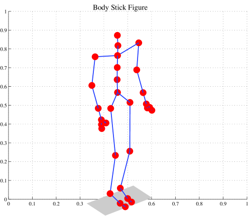
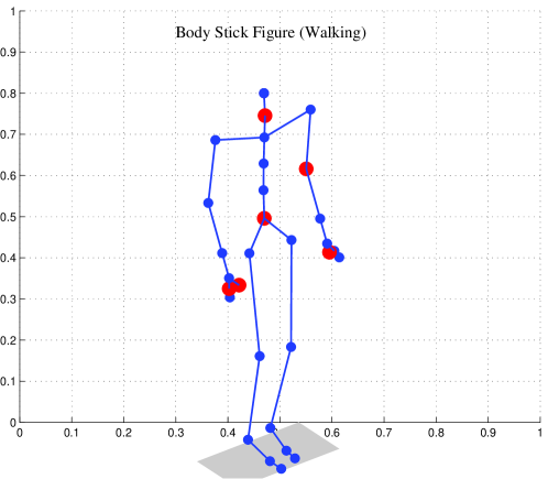
  Figure 1: A stick-figure of the human body showing $41$ markers (red spheres) placed on different parts of the body in order to capture the motion data. Captured data are related to movements of the different joints during the human’s basic activities.

• PCA-DTW-KNN: For the dimension reduction experiment in section 3.6, we compare the low-rank representation found by low-rank LMNN with a dimensionality reduction by classical Principle Component Analysis (PCA) [32]. Thereby, PCA is applied directly to the vectorial sequence entries from the training set. Afterward, DTW is applied on the first 3 principal components of the data, followed by a KNN classifier.

We use $10$-fold cross-validations with $10$ repetitions for evaluation. All experiments are carried out using the same cross-validation partitions.

For evaluation and comparison of the proposed approach, we consider $3$ different Mocap databases based on human motions. These data give rise to the following four different training sets:

3.2 CMU Mocap dataset:

We use the Human motion capture dataset from the CMU graphics laboratory [33]. The data is captured by Vicon infra-red cameras using $41$ markers placed at different parts of the body, close to the joints (Fig.1). Afterward, the images are augmented to 3D data and transferred to kinematic information such as joint rotation/translation based on skeleton information. The result consists of $62$ body features leading to $62$-dimensional time series with a high correlation of their dimensions. We select two classification scenarios from the full data set to investigate different aspects of the proposed method.

• Walking: This dataset contains data from $7$ different walking styles (normal, fast, slow, turn right, turn left, veer right and veer left) carried out by $4$ different subjects. the dataset consists of $49$ samples ($7$ samples per class) with a $62$-dimensional representation.

• Dance: We use $35$ samples of data related to two different styles of dancing: Modern and Indian; these are available from CMU graphics laboratory as participant subjects $5$ and $94$ [33]. Each class contains various dance performances related to subcategories of the class; as a result, the variations among the data within the classes produce overlapping between the two classes, which makes the classification very challenging.

Figure 2: Eigenvalue profile sorted according to the size of the eigenvalues of matrix $\mathbf{L}$. The green circle indicates the selected dimension as the effective dimension for the regularised coefficients.

3.3 Cricket Umpire’s Signals

Cricket as a bat-and-ball team game is the world’s second most popular sport[34]. An umpire is a person in the game who makes decisions and announces different events going on on the cricket field. The umpire communicates using his arm movements. As an example, the event ‘No-Ball’ is signaled by holding one arm out at shoulder height to indicate that the ball is delivered along with the player’s fault(s); in order to announce the start of the last hour of the play, the umpire taps his wrist and his watch [35].

For our classification task, we use the dataset which is provided by [36]. This dataset contains $12$ umpire signals, each performed by four different persons in $3$ to $4$ repetitions. Data are captured via accelerometers on the umpire’s wrists while performing the signals[37]. This way, data sequences are recorded in a 3D spatial format (with $X$, $Y$, and $Z$ coordination) providing $6$ features per time step for the classification task. The classification task is to distinguish between $12$ classes of different cricket umpire’s signals using the available $6$ motion features and a total number of $180$ data samples.

Table 1: Classification accuracy(%) for the proposed DTW-LMNN approach and its comparison to the regular Euclidean-LMNN and DTW-kNN methods for the four data sets. Variances are reported in parentheses, and a paired t-test checks the hypothesis that DTW-KNN and DTW-LMNN do not differ.

	Euclidean LMNN	DTW-KNN	DTW-LMNNN	p-value
Walking	92 (0.87)	95 (0.77)	100 (0)	–
Dance	80 (1.49)	77.5 (1.51)	90 (1.03)	0.01
Cricket Signals	95.56 (0.38)	99.44 (0.18)	100 (0)	–
Words	97.30 (1.20)	98.61 (1.05)	99.06 (1.11)	$<0.01$

Table 2: Accuracy of the KNN classifier used for low-rank data/distance representations as obtained by PCA, low-rank Euclidean LMNN, and low-rank LMNN with DTW, choosing rank $3$. A paired t-test evaluates the hypothesis that the results of a PCA projection together with DTW and LMNN are the same as low-rank DTW-LMNN learning.

	low-rank Euclidean LMNN	PCA with DTW-KNN	low-rank DTW-LMNNN	p-value
Walking	86.6 (1.10)	96 (1.08)	98.8 (1.80)	$<0.01$
Dance	75 (1.52)	76 (1.51)	95 (0.80)	0.012
Cricket Signals	96.11 (0.46)	99.44 (0.18)	100 (0)	–
Words	98.60 (0.14)	94.24 (0.25)	99.12 (0.17)	$<0.01$

3.4 Articulatory Words

People can have oral communication difficulties based on different reasons; one example is the treatment of larynx cancer via surgery, after which it is probable that the patient has significant vocal impairments. One practical solution to facilitate this issue is to benefit from silent ‘speech’ recognition [38, 39, 40]: this technology uses facial data (such as lips and tongue movements) to recognize the person’s voiceless uttered words or phrases [39]. The required motion information can be captured by attaching Electromagnetic Articulograph (EMA) sensors to the person’s articulators such as lips and tongues [41]. The given task is to classify the uttered word from this movement data reliably.

For our experiments, we use the articulatory dataset from [38], which consists of EMA data related to $25$ words uttered by different native English speakers. For the motion capture process, $12$ EMA sensors are used to capture the 3D information ($X$, $Y$, and $Z$ positions) of various facial organs as time series data. As it is explained in [38], the sensors are placed at different parts of forehead, lips, and tongues shaping up $36$ available features, out of which we use $9$ specific dimensions for our classification task collected from markers on the tongue tip, the upper lip, and lower lip. More precisely, we used the 3D spatial data ($X$, $Y$, and $Z$) related to the tip of the tongue (T1), upper lip (UL) and lower lip (LL) which results in $9$ features in total [42]. Hence the classification task can be characterized as categorizing $25$ classes of different words using $575$ samples of data which are represented based on $9$ motion-based features.

3.5 Classification Accuracy

In this section, we study the proposed methods as concerns their classification accuracies. We compare the classification accuracy of the DTW-LMNN algorithm, Euc-LMNN, and DTW-KNN. We accompany the resulting accuracies by the variance, and by the p-value from a paired t-test testing the hypothesis that plain DTW and the metric adaptation technique DTW-LMNN yield the same result [43]. All results from the classification task are displayed in Table 1.

According to the classification results 1, DTW-LMNN outperforms the Euclidean version of the algorithm for all data sets. This observation supports the expectation that DTW constitutes a suitable dissimilarity measure for motion data due to its ability to account for different motion durations. From another point of view, metric adjustment enables an improvement of the classification accuracy for all cases. Interestingly, it causes a slight superiority of the Euclidean metric as compared to DTW without metric adjustment for the dance dataset. For all settings, metric adjustment leads to an improvement of the classification in connection to DTW.

Figure 3: Classification accuracy for training and test set of the dance dataset based on regularized coefficients. The green diamond represents the highest accuracy for the test set for $12$ effective dimensions. The green circle refers to the non-regularized coefficients, and the triangle to only one effective dimension.

3.6 low-rank matrix representation

We study the dimensionality reduction performance of DTW-LMNN using the datasets introduced in section 3, in order to obtain a compressed representation of the data for the classification tasks. As discussed in section 2 we can use a low-rank matrix $\mathbf{M}$ or $\mathbf{L}$, corresponding to low-rank constraints in the optimization problem (Eq. 7). Apart from a compressed representation, this can lead to a significant increase in the time performance of the kNN classification in the low-dimensional projection space [44]. We use a rank $3$ matrix $\mathbf{L}$ corresponding to a projection into the space $\mathbb{R}^{3}$. For comparison, we also investigate the effect of a rank restriction for the Euclidean version of LMNN, and we investigate the result of classical PCA for dimensionality reduction of the data before classification. The results of these low-rank classification pipelines are reported in Table 2.

Figure 4: Average (blue bars) and deviation (red lines) of the relevance values for features of the dance dataset calculated according to the normalised diagonal values of $(\mathbf{L}^{t}\mathbf{L})$. Top: Regularised relevance profile. Bottom: Non-regularised relevance profile.

As reported in Table 2, low rank DTW-LMNN preserves the good classification accuracy of DTW-LMNN for the reported data sets. In contrast, PCA does not achieve the same accuracy, nor does Euclidean LMNN. Interestingly, rank restrictions improve the classification accuracy for DTW-LMNN for the Dance data set. Conversely, PCA reduces the classification accuracy for the Articulatory words data set. Hence projection directions which are learned by LMNN optimization can enhance the discriminative aspects of DTW alignment for a low-rank matrix representation. As an interesting point in the results, the DTW-LMNN algorithm managed to classify the Cricket dataset with $100\%$ accuracy while obtaining a compressed representation as well.

3.7 Regularized Relevance Profile:

In this section, we investigate the resulting relevance profiles for two of the introduced datasets for the metrics obtained by DTW-LMNN. We restrict the analysis to DTW-LMNN due to its superior performance for all data sets. Further, we investigate only two of the four datasets to focus on the notable effects of the matrix regularization. The data sets Articulatory Words and Cricket Signals are of minor interest for this section due to their comparably low-dimensionality ($9$ and $6$ sensors only, without considerable correlations). On the contrary, the two human body datasets (Dance and Walking) have a high number of features ($62$) with substantial correlations among the joints. Hence we can expect interesting effects when regularizing the learned matrix.

Matrix regularization has different effects: (I) It enables a valid interpretation of the feature relevance profile since it avoids spurious relevance peaks and random effects due to data correlations – we evaluate this effect by an inspection of the sparsity and variance of the relevance profile within cross-validation. (II) It suggests the possible ways to reduce the data dimensionality by eliminating the most irrelevant features according to the found relevance profile. We investigate this effect by evaluating the classification performance if the feature dimensions are iteratively deleted according to their relevance.

Figure 5: Classification performance of dance dataset based on the selected features according to the regularised profile

3.7.1 Dance dataset

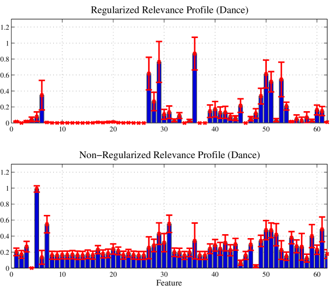
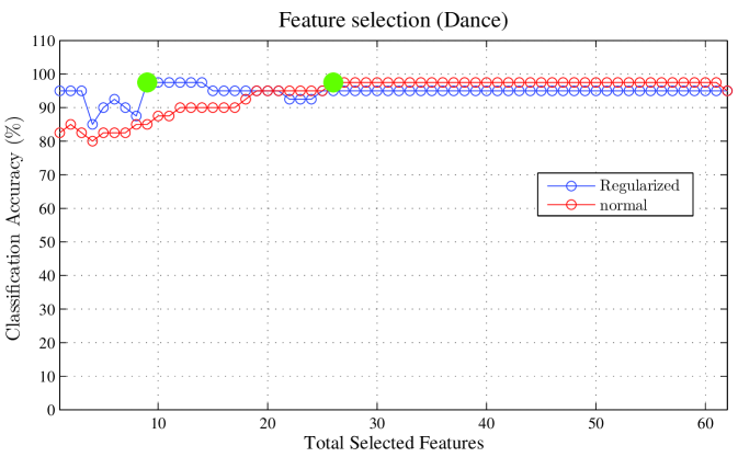
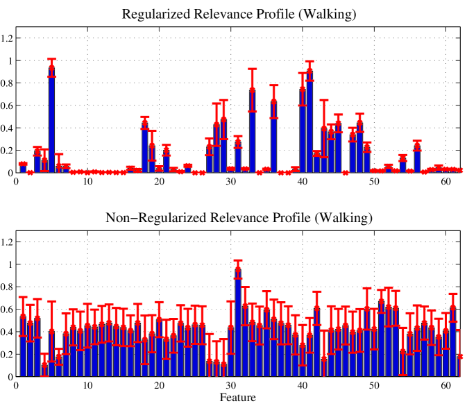
For the dance dataset, we calculate the relevance value of features as $\mathrm{diag}(\mathbf{L}^{t}\mathbf{L})$ based on the transformation matrix $\mathbf{L}$ which is obtained via DTW-LMNN, see section 3.5. For the graphical display, we normalize the profiles to the range $[0,1]$. Since $\mathbf{L}$ is different for different cross-validation partitions, we report the average and variance of each diagonal value. The resulting relevance profile without regularization is displayed in Fig. 4-bottom. The total variance of this profile is $4.47$.

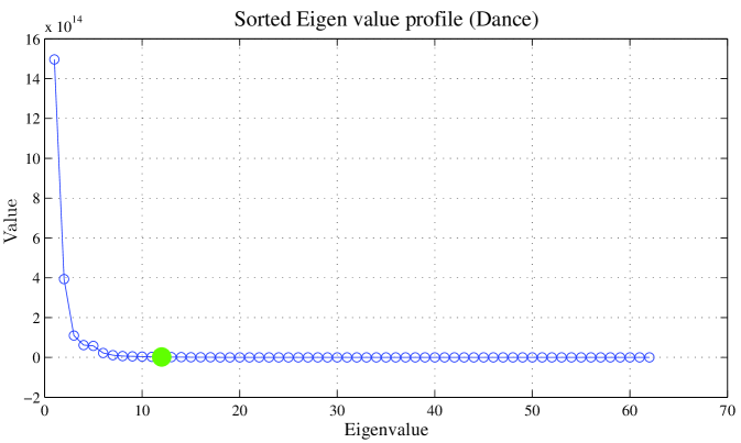
In comparison, we regularize the matrix $\mathbf{L}$ according to Eq. 12. Thereby, the eigenvectors $\vec{u}^{i}$ of the vectors of the distance matrix $\mathbf{D}$ for the eigenvalue $0$ are determined based on the training set. We report the result for the choice of $12$ effective dimensions of the eigenvectors by showing the corresponding eigenvalue profile in Fig. 2. The resulting regularized profile is shown in Fig. 3-top. Clearly, much fewer features are singled out as relevant. Further, the variance of the profile is reduced to $2.86$.

Figure 6: Stick figure of different body parts related to the dance dataset. Red markers are the selected important inputs according to the regularised relevance profile of the features.

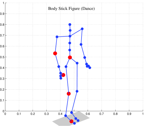
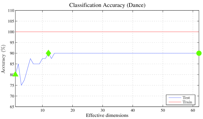
We test the ability of metric learning to induce a feature selection by sorting the input dimensions (features) according to their relevance values in each of the two relevance profiles in Fig. 4. Then we select the important features according to this order and report the resulting classification accuracy on the test set (Fig. 5). Interestingly, both relevance profiles let us to remove a large number of sensors without a reduction of the classification accuracy. This feature reduction can be iterated until only $9$ features are left for the regularized profile, and $26$ features for the non-regularized one. Hence regularization greatly enhances the feature selection ability of the technique. The resulting $9$ features are displayed based on the skeleton information in Fig. 6. The semantic meaning of these features is reported in Table. 3.

Table 3: Total variance in the regularized and non-regularized relevance profiles along with the feature selection results for the Dance dataset.

Total variance of profile (before regularization): 4.47

Total variance of regularized profile: 2.86

Selected Joints and related feature number: rhumerus(27,28,29),

rthumb(36), rfemur(49,50,51), rfoot(53) and root(6)

According to Fig. 4, the regularization matrix has positive effects on the relevance profile. While it retains the classification performance at its highest rate (see Fig. 3), it reduces redundancy in the profile and produces a sparse representation for the relevance values of inputs (features). Besides, based on the variance measure for the relevance profile over different cross-validation partitions, the regularized profile has less variance and thus is more reliable than the normal one.

As a semantic interpretation, it can be concluded from Fig. 6 that hands and feet are both important discriminative features for this dancing task. From another point of view, this is a difficult task because each class has different subcategories within itself which account for overlaps with other class; hence the combination of both (hand and foot) is required to distinguish between the two dance categories. Furthermore, as another interesting semantic interpretation, only the data related to one side of the body (right side) is necessary to achieve the highest classification performance. This interpretation coincides with the fact that dancing is typically a symmetrical whole body movement in which symmetry can be found between the left and right sides of the body.

3.7.2 Walking dataset

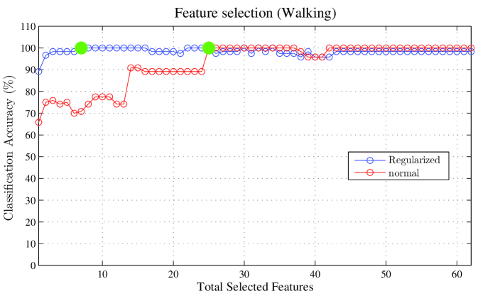
We repeat this experimental setting for the walking dataset, which leads to $14$ effective dimensions selected from the regularization matrix. The obtained regularized profile can be seen in Fig. 7. The total variances of the relevance profiles before and after the regularization are $10.7$ and $2.51$, respectively. Again, similar to the dance dataset, the most relevant features, and the resulting classification accuracies are displayed in Fig. 8. The essential joints are listed in Tab. 4.

Figure 7: Average (blue bars) and deviation (red lines) of the relevance values for features of the Walking dataset calculated according to the normalised diagonal values of $(\mathbf{L}^{t}\mathbf{L})$. Top: Regularised relevance profile. Bottom: Non-regularised relevance profile.

Table 4: Total variance of the regularized and non-regularized relevance profiles and selected features for the Walking dataset.

Total variance of plain profile: 10.70

Total variance of regularized profile: 2.51

Selected Joints and feature number: root(5), lhumerus(40,41),

rhand(33), rthumb(36), lowerneck(18) and lthumb (48)

Similar to the results for the dance dataset, regularization of the learned metric results in a sparse representation of the relevance profile and a reduced variance. Furthermore, according to Fig. 8, a classification accuracy of $100\%$ can be achieved while choosing fewer features ($7$ features for the regularized profile instead of $25$ for the standard one).

Based on the observations from Fig. 9, for this dataset (and this classification task), hands are more important than feet. In addition, as the classes are very similar (all of them are connected to walking), the classification algorithm also needs some information about both sides of the body in order to carry out the classification task with a perfect result. We tested this hypothesis by using Lhand instead of Rhand or deleting Rthumb (since we already have Lthumb), but in both cases, the performance decreased (around $3$ to $4\%$) showing that those selected features are all necessary even though they are symmetrical in the skeleton structure.

According to the results given in section 3.7, after applying the regularization matrix, both datasets showed improved results. The regularization enhances the reliability of the relevance profiles, corresponding to a smaller variance. In addition, regularization enables a more efficient feature selection strategy.

Figure 8: Classification performance of walking dataset based on the selected features according to the regularised profile

Figure 9: Stick figure of different body parts related to the walking dataset. Red markers are the selected important inputs according to the regularised relevance profile of the features.

4 Conclusions and Future Work

In this paper we introduced a distance based extension (DTW-LMNN) to the popular metric learning method LMNN in a very generic way, opening up the possibility to also transfer auxiliary concepts such as metric regularization. This framework enables us to benefit from the DTW dissimilarity measure which is particularly suited to the analysis of Mocap data. While dealing with multi-dimensional motion data such as human movements, the component-wise dissimilarity values achieved by the DTW measure can be treated as different features to obtain a semi-vectorial representation for the dissimilarities among the data. Therefore, the representation can be combined with the LMNN framework to efficiently adapt the feature ranking and correlation according to the classification tasks at hand. The mentioned dissimilarity representation for the motion data also conserves the convexity of the optimization problem Eq.3.

The strong results achieved with DTW-LMNN show that augmenting the LMNN approach with the DTW dissimilarity measure can significantly improve the metric learning performance. For both, classification and dimensionality reduction tasks, the proposed approach outperforms the Euclidean version of LMNN as well as the DTW based K-nearest neighbor method. Therefore, it can be concluded that DTW-LMNN can benefit from the strength of the DTW dissimilarity metric and LMNN metric learning together. According to our encouraging results across diverse motion-based benchmarks, the DTW-LMNN framework offers a suitable discriminative method to achieve high-performance classifications and compressed representations dealing with motion-based datasets.

As another contribution of this paper, we devised a way to transfer the concept of metric regularization to alignment based representations; this concept has recently been proposed for the vectorial case[26]. According to the results in section 3.7, this regularization step is a crucial prerequisite for a valid interpretation of the relevance profile. To that end, we managed to use the dissimilarity-based information in order to remove the highly correlated dimensions related to the null space contributions. According to the results, the dissimilarity-based regularization brings significant effects to the relevance profile; further, it increases the semantic interpretability of the resulting discriminative models. It is important to mention that the proposed regularization step can be applied to any other dissimilarity-based metric framework as well.

Relying on these promising results achieved by the proposed DTW-LMNN framework, there is considerable potential for future research in dissimilarity-based metric learning: the principle can be transferred to other metric learning methods which are not linked to KNN. In addition to that, a promising research line could be to investigate more advanced regularization techniques to achieve a further enriched relevance profile, such as proposed in [25].

References

- [1] B. Hosseini and B. Hammer. Efficient metric learning for the analysis of motion data. In IEEE International Conference on Data Science and Advanced Analytics (DSAA), 2015.
- [2] Ian Spiro, Thomas Huston, and Christoph Bregler. Markerless motion capture in the crowd. CoRR, abs/1204.3596, 2012.
- [3] Yebin Liu, Juergen Gall, Carsten Stoll, Qionghai Dai, Hans-Peter Seidel, and Christian Theobalt. Markerless motion capture of multiple characters using multiview image segmentation. IEEE Trans. Pattern Anal. Mach. Intell., 35(11):2720–2735, 2013.
- [4] Christoph Bregler. Kinematic motion models. In Computer Vision, A Reference Guide, pages 437–440. 2014.
- [5] Jong Sze Joon. Reviewing principles and elements of animation for motion capture-based walk, run and jump. In Computer Graphics, Imaging and Visualization (CGIV), 2010 Seventh International Conference on, pages 55–59, Aug 2010.
- [6] Andrea Fossati, Juergen Gall, Helmut Grabner, Xiaofeng Ren, and Kurt Konolige, editors. Consumer Depth Cameras for Computer Vision, Research Topics and Applications. Advances in Computer Vision and Pattern Recognition. Springer, 2013.
- [7] Arjun Jain, Jonathan Tompson, Yann LeCun, and Christoph Bregler. Modeep: A deep learning framework using motion features for human pose estimation. In Computer Vision - ACCV 2014 - 12th Asian Conference on Computer Vision, Singapore, Singapore, November 1-5, 2014, Revised Selected Papers, Part II, pages 302–315, 2014.
- [8] Birgitta Burger and Petri Toiviainen. MoCap Toolbox – A Matlab toolbox for computational analysis of movement data. In Roberto Bresin, editor, Proceedings of the 10th Sound and Music Computing Conference, pages 172–178, Stockholm, Sweden, 2013. KTH Royal Institute of Technology.
- [9] A.W. Vieira, T. Lewiner, W.R. Schwartz, and M. Campos. Distance matrices as invariant features for classifying mocap data. In Pattern Recognition (ICPR), 2012 21st International Conference on, pages 2934–2937, Nov 2012.
- [10] Jan Sedmidubsky and Jakub Valcik. Retrieving similar movements in motion capture data. In Nieves Brisaboa, Oscar Pedreira, and Pavel Zezula, editors, Similarity Search and Applications, volume 8199 of Lecture Notes in Computer Science, pages 325–330. Springer Berlin Heidelberg, 2013.
- [11] Bastian Demuth, Tido Röder, Meinard Müller, and Bernhard Eberhardt. An information retrieval system for motion capture data. In Mounia Lalmas, Andy MacFarlane, Stefan M. Rüger, Anastasios Tombros, Theodora Tsikrika, and Alexei Yavlinsky, editors, Advances in Information Retrieval, 28th European Conference on IR Research, ECIR 2006, London, UK, April 10-12, 2006, Proceedings, volume 3936 of Lecture Notes in Computer Science, pages 373–384. Springer, 2006.
- [12] Feng Zhou and Fernando De la Torre Frade. Generalized time warping for multi-modal alignment of human motion. In IEEE Conference on Computer Vision and Pattern Recognition (CVPR), June 2012.
- [13] K. Adistambha, C.H. Ritz, and I.S. Burnett. Motion classification using dynamic time warping. In Multimedia Signal Processing, 2008 IEEE 10th Workshop on, pages 622–627, Oct 2008.
- [14] François Petitjean, Germain Forestier, Geoffrey I. Webb, Ann E. Nicholson, Yanping Chen, and Eamonn J. Keogh. Dynamic time warping averaging of time series allows faster and more accurate classification. In Ravi Kumar, Hannu Toivonen, Jian Pei, Joshua Zhexue Huang, and Xindong Wu, editors, 2014 IEEE International Conference on Data Mining, ICDM 2014, Shenzhen, China, December 14-17, 2014, pages 470–479. IEEE, 2014.
- [15] Mark P. Styczynski, Kyle L. Jensen, Isidore Rigoutsos, and Gregory Stephanopoulos. BLOSUM62 miscalculations improve search performance. Nature Biotechnology, 26(3):274–275, March 2008.
- [16] Robert C. Edgar. Optimizing substitution matrix choice and gap parameters for sequence alignment. BMC Bioinformatics, 10:396, 2009.
- [17] L. Boyer, Y. Esposito, A. Habrard, J. Oncina, and M. Sebban. Sedil: Software for edit distance learning. Lect. Notes Comput. Sci., 5212 LNAI(2):672–677, 2008.
- [18] Aurélien Bellet, Amaury Habrard, and Marc Sebban. A survey on metric learning for feature vectors and structured data. CoRR, abs/1306.6709, 2013.
- [19] Brian Kulis. Metric learning: A survey. Foundations and Trends in Machine Learning, 5(4):287–364, 2013.
- [20] Petra Schneider, Michael Biehl, and Barbara Hammer. Adaptive relevance matrices in learning vector quantization. Neural Computation, 21(12):3532–3561, 2009.
- [21] Kilian Q. Weinberger and Lawrence K. Saul. Distance metric learning for large margin nearest neighbor classification. Journal of Machine Learning Research, 10:207–244, 2009.
- [22] Michael Biehl, Kerstin Bunte, and Petra Schneider. Analysis of flow cytometry data by matrix relevance learning vector quantization. Plos One, 8(3), 2013.
- [23] Andreas Backhaus and Udo Seiffert. Classification in high-dimensional spectral data: Accuracy vs. interpretability vs. model size. Neurocomputing, 131:15–22, 2014.
- [24] Kerstin Bunte, Petra Schneider, Barbara Hammer, Frank-Michael Schleif, Thomas Villmann, and Michael Biehl. Limited rank matrix learning, discriminative dimension reduction and visualization. Neural Networks, 26:159–173, 2012.
- [25] Benoît Frénay, Daniela Hofmann, Alexander Schulz, Michael Biehl, and Barbara Hammer. Valid interpretation of feature relevance for linear data mappings. In 2014 IEEE Symposium on Computational Intelligence and Data Mining, CIDM 2014, Orlando, FL, USA, December 9-12, 2014, pages 149–156. IEEE, 2014.
- [26] Marc Strickert, Barbara Hammer, Thomas Villmann, and Michael Biehl. Regularization and improved interpretation of linear data mappings and adaptive distance measures. In IEEE Symposium on Computational Intelligence and Data Mining, CIDM 2013, Singapore, 16-19 April, 2013, pages 10–17. IEEE, 2013.
- [27] M. Bernard, L. Boyer, A. Habrard, and M. Sebban. Learning probabilistic models of tree edit distance. Pattern Recognition, 41(8):2611–2629, 2008.
- [28] Bassam Mokbel, Benjamin Paaßen, Frank-Michael Schleif, and Barbara Hammer. Metric learning for sequences in relational lvq. Neurocomputing, (accepted/in press), 2015.
- [29] E. Pekalska and B. Duin. The Dissimilarity Representation for Pattern Recognition. Foundations and Applications. World Scientific, 2005.
- [30] Ghazi Al-Naymat, Sanjay Chawla, and Javid Taheri. Sparsedtw: A novel approach to speed up dynamic time warping. CoRR, abs/1201.2969, 2012.
- [31] W. Arlt, M. Biehl, A. E. Taylor, S. Hahner, R. Libe, B. A. Hughes, P. Schneider, D. J. Smith, H. Stiekema, N. Krone, E. Porfiri, G. Opocher, J. Bertherat, F. Mantero, B. Allolio, M. Terzolo, P. Nightingale, C. H. L. Shackleton, X. Bertagna, M. Fassnacht, and P. M. Stewart. Urine steroid metabolomics as a biomarker tool for detecting malignancy in adrenal tumors. J Clinical Endocrinology and Metabolism, 96:3775–3784, 2011.
- [32] Ian Jolliffe. Principal component analysis. Wiley Online Library, 2002.
- [33] CMU. Carnegie mellon university graphics lab: Motion cap- ture database. http://mocap.cs.cmu.edu, Mar. 2007.
- [34] Khabir Uddin Mughal. Top 10 most popular sports in the world. http://sporteology.com/top-10-popular-sports-world/. Published: 2015-03-07.
- [35] D Shepherd. Bbc sport academy cricket umpire signals. 2005.
- [36] M. H. Ko, G. W. West, S. Venkatesh, and M. Kumar. Online context recognition in multisensor systems using dynamic time warping. In ISSNIP’05, pages 283–288. IEEE, 2005.
- [37] Graeme S Chambers, Svetha Venkatesh, Geoff AW West, and Hung Hai Bui. Segmentation of intentional human gestures for sports video annotation. In Multimedia Modelling Conference, 2004. Proceedings. 10th International, pages 124–129. IEEE, 2004.
- [38] Jun Wang, Arvind Balasubramanian, Luis Mojica de La Vega, Jordan R Green, Ashok Samal, and Balakrishnan Prabhakaran. Word recognition from continuous articulatory movement time-series data using symbolic representations. In SLPAT’13 Workshop, pages 119–127, 2013.
- [39] Jun Wang, Ashok Samal, and Jordan Green. Preliminary test of a real-time, interactive silent speech interface based on electromagnetic articulograph. In SLPAT’14, pages 38–45, 2014.
- [40] Jun Wang, Ashok Samal, Jordan R Green, and Frank Rudzicz. Whole-word recognition from articulatory movements for silent speech interfaces. 2012.
- [41] Yana Yunusova, Jordan R Green, and Antje Mefferd. Accuracy assessment for ag500, electromagnetic articulograph. Journal of Speech, Language, and Hearing Research, 52(2):547–555, 2009.
- [42] Mohammad Shokoohi-Yekta, Bing Hu, Hongxia Jin, Jun Wang, and Eamonn Keogh. On the non-trivial generalization of dynamic time warping to the multi-dimensional case. In SDM, 2015.
- [43] Mary C Seiler and Fritz A Seiler. Numerical recipes in c: the art of scientific computing. Risk Analysis, 9(3):415–416, 1989.
- [44] Kilian Q Weinberger and Lawrence K Saul. Fast solvers and efficient implementations for distance metric learning. In Proceedings of the 25th international conference on Machine learning, pages 1160–1167. ACM, 2008.