Entanglement distribution and quantum discord

Abstract

Establishing entanglement between distant parties is one of the most important problems of quantum technology, since long-distance entanglement is an essential part of such fundamental tasks as quantum cryptography or quantum teleportation. In this lecture we review basic properties of entanglement and quantum discord, and discuss recent results on entanglement distribution and the role of quantum discord therein. We also review entanglement distribution with separable states, and discuss important problems which still remain open. One such open problem is a possible advantage of indirect entanglement distribution, when compared to direct distribution protocols.

I Introduction

This lecture presents an overview of the task of establishing entanglement between two distant parties (Alice and Bob) and its connection to quantum discord Ollivier and Zurek (2001); Henderson and Vedral (2001); Modi et al. (2012); Streltsov (2015); Adesso et al. (2016). Surprisingly, it is possible for the two parties to perform this task successfully by exchanging an ancilla which has never been entangled with Alice and Bob. This puzzling quantum protocol was already suggested in Cubitt et al. (2003), but a thorough study Streltsov et al. (2012a); Chuan et al. (2012); Kay (2012); Streltsov et al. (2014, 2015a); Zuppardo et al. (2016) and experimental verification Fedrizzi et al. (2013); Vollmer et al. (2013); Peuntinger et al. (2013) (see also Silberhorn (2013)) had to wait for almost ten years until recently, when interest in general quantum correlations arose and led to insights about their role in the entanglement distribution protocol.

A composite quantum system does not need to be in a product state for the subsystems, but it can also occur as a superposition of product states, or as a mixture of such superpositions. This feature does not exist in the classical world, and a state exhibiting it is called entangled. In general, a state is said to contain entanglement if it cannot be written as a mixture of projectors onto product states. It is said to contain quantum correlations, if it cannot be written as a mixture of projectors onto product states with local orthogonality properties. And it is said to contain correlations (classical or quantum), if it cannot be written as a product state.

Let us formalize these notions. In the following definitions we will consider for simplicity only bipartite quantum systems (with superscripts $A$ and $B$ for Alice and Bob, respectively); the generalization to composite quantum systems with more than two subsystems is straightforward. Let us denote by $\{\ket{e_{i}}\}$ a complete set of orthogonal basis states (which could also be interpreted as classical states), i.e. $\braket{e_{i}}{e_{j}}=\delta_{ij}$, while Greek letters indicate quantum states which are not necessarily orthogonal, i.e., for the ensemble $\{\ket{\psi_{i}}\}$ in general $\braket{\psi_{i}}{\psi_{j}}\neq\delta_{ij}$ holds.

A separable state $\rho_{\mathrm{sep}}$ can be written as Werner (1989)

$$\rho_{\mathrm{sep}}^{AB}=\sum_{i,j}p_{ij}\ket{\psi_{i}}\!\bra{\psi_{i}}^{A}\otimes\ket{\phi_{j}}\!\bra{\phi_{j}}^{B},$$ (1)

where $p_{ij}$ are probabilities with $\sum_{i,j}p_{ij}=1$. The set of all separable states will be denoted by $\mathcal{S}$. Any separable state can be produced with local operations and classical communication (LOCC). An entangled state cannot be written as in Eq. (1). In order to produce an entangled state, a non-local operation is needed. In Section II we will review different ways to quantify the amount of entanglement in a given state.

A state is called classically correlated (CC) if it can be written as Piani et al. (2008)

$$\rho_{\mathrm{cc}}^{AB}=\sum_{i,j}p_{ij}\ket{e_{i}}\!\bra{e_{i}}^{A}\otimes\ket{e_{j}}\!\bra{e_{j}}^{B},$$ (2)

with $\braket{e_{i}}{e_{j}}=\delta_{ij}$. Measuring $\rho_{\mathrm{cc}}$ in the local bases $\{\ket{e_{i}}^{A}\}$ and $\{\ket{e_{j}}^{B}\}$ does not change the state, i.e.,

$$\Pi^{A}\otimes\Pi^{B}[\rho_{\mathrm{cc}}^{AB}]=\rho_{\mathrm{cc}}^{AB},$$ (3)

where the von Neumann measurement $\Pi$ is defined as

$$\Pi[\sigma]=\sum_{i}\ket{e_{i}}\!\bra{e_{i}}\sigma\ket{e_{i}}\!\bra{e_{i}}.$$ (4)

The set of all classically correlated states will be denoted by $\mathcal{CC}$. A quantum correlated state cannot be written as in Eq. (2). The eigenbasis of a quantum correlated state is not a product basis with the property that the sets of local states are orthogonal ensembles.

It is also possible to combine the aforementioned frameworks of separability and classicality, thus arriving at classical-quantum (CQ) states Piani et al. (2008):

$$\rho_{\mathrm{cq}}^{AB}=\sum_{i,j}p_{ij}\ket{e_{i}}\bra{e_{i}}^{A}\otimes\ket{\psi_{j}}\bra{\psi_{j}}^{B}.$$ (5)

The set of all classical-quantum states will be denoted by $\mathcal{CQ}$. For any CQ state, there exists a local von Neumann measurement on the subsystem $A$ which leaves the state unchanged, i.e.,

$$\Pi^{A}\otimes\openone^{B}[\rho_{\mathrm{cq}}^{AB}]=\rho_{\mathrm{cq}}^{AB},$$ (6)

where the von Neumann measurement $\Pi$ is given in Eq. (4). If a state cannot be written as in Eq. (5), we say that the state has nonzero quantum discord with respect to the subsystem $A$. Measuring a state with nonzero discord in any orthogonal basis on the subsystem $A$ necessarily changes the state. In Section III we will present different ways to quantify the amount of discord in a given state.

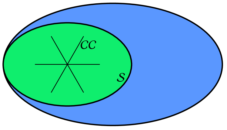
Figure 1: State space for composite quantum systems Ferraro et al. (2010): classically correlated states form a connected set $\mathcal{CC}$ of measure zero; separable states form a convex set $\mathcal{S}$ (green, containing $\mathcal{CC}$). Quantum correlated states are all states outside of $\mathcal{CC}$, and entangled states (blue) are all states outside of $\mathcal{S}$.

From the above definitions it is clear that classically correlated states are a subset of separable states, and that entangled states are a subset of quantum correlated states. These different types of states for composite quantum systems therefore form a nested structure Ferraro et al. (2010) which is sketched in Fig. 1. Note that separable states form a convex set, due to their definition in Eq. (1). However, classically correlated states do not form a convex set: one can produce a quantum correlated state by mixing two classically correlated states.

Those states which are not entangled, but nevertheless possess quantum correlations a la discord, may exhibit puzzling features. They can be produced via LOCC, but nevertheless they carry quantum properties. Namely, in order to produce them one has to create quantumness in the form of non-orthogonality. This makes them a potential resource for quantum information processing protocols. Counterintuitively, even though they do not carry entanglement, they may be used for the distribution of entanglement, as we will see below.

The structure of this lecture is as follows: in Section II we review different measures of quantum entanglement, discord quantifiers are reviewed in Section III. In Section IV we review recent results on entanglement distribution and discuss the role of quantum discord therein. Conclusions in Section V complete our lecture.

II Quantum entanglement

Here, we will review different entanglement measures, mainly focusing on measures which are used in this lecture. More detailed reviews, also containing other entanglement measures, can be found in Bruß (2002); Plenio and Virmani (2007); Horodecki et al. (2009). In general, we require that a measure of entanglement $\mathcal{E}$ fulfills the following two properties Vedral et al. (1997); Vedral and Plenio (1998):

• Nonnegativity: $\mathcal{E}(\rho)\geq 0$ for all states $\rho$ with equality for all separable states ,

• Monotonicity: $\mathcal{E}(\Lambda[\rho])\leq\mathcal{E}(\rho)$ for any LOCC operation $\Lambda$.

Many entanglement measures also have additional properties such as strong monotonicity in the sense that entanglement does not increase on average under selective LOCC operations Vedral et al. (1997); Vedral and Plenio (1998): $\sum_{i}p_{i}\mathcal{E}(\sigma_{i})\leq\mathcal{E}(\rho)$, where the states $\sigma_{i}$ are obtained from the state $\rho$ by the means of LOCC with the corresponding probabilities $p_{i}$. Moreover, many entanglement measures are also convex in the state, i.e., $\mathcal{E}(\sum_{i}p_{i}\rho_{i})\leq\sum_{i}p_{i}\mathcal{E}(\rho_{i})$ Vedral et al. (1997); Vedral and Plenio (1998).

From now on we will focus on the bipartite scenario with two parties $A$ and $B$ of the same dimension $d$. In this case, any entanglement measure is maximal on states of the form

$$\ket{\phi_{d}^{+}}=\frac{1}{\sqrt{d}}\sum_{i=0}^{d-1}\ket{ii},$$ (7)

since from this state any quantum state can be created via LOCC operations Horodecki et al. (2009). Of particular importance is the two-qubit singlet state $(\ket{01}-\ket{10})/\sqrt{2}$, which can be obtained from the state $\ket{\phi_{2}^{+}}$ via local unitaries. In entanglement theory local unitaries do not change the properties of a state, and thus we will refer to the state $\ket{\phi_{2}^{+}}$ as a singlet.

Operational measures of entanglement are distillable entanglement and entanglement cost. Distillable entanglement quantifies the maximal rate for extracting singlets from a state via LOCC operations Plenio and Virmani (2007); Horodecki et al. (2009):

$$\mathcal{E}_{\mathrm{d}}(\rho)=\sup\left\{R:\lim_{n\rightarrow\infty}\left(\inf_{\Lambda}\left\|\Lambda\left[\rho^{\otimes n}\right]-\left(\phi_{2}^{+}\right)^{\otimes nR}\right\|_{1}\right)=0\right\},$$ (8)

where $||M||_{1}=\mathrm{Tr}\sqrt{M^{\dagger}M}$ is the trace norm, $\phi_{2}^{+}$ is the projector onto the state $\ket{\phi_{2}^{+}}$ , and the infimum is performed over all LOCC operations $\Lambda$. Entanglement cost on the other hand quantifies the minimal singlet rate required for creating a state via LOCC operations Plenio and Virmani (2007); Horodecki et al. (2009):

$$\mathcal{E}_{\mathrm{c}}(\rho)=\inf\left\{R:\lim_{n\rightarrow\infty}\left(\inf_{\Lambda}\left\|\Lambda\left[\left(\phi_{2}^{+}\right)^{\otimes nR}\right]-\rho^{\otimes n}\right\|_{1}\right)=0\right\}\,.$$ (9)

For pure states $\ket{\psi}=\ket{\psi}^{AB}$ these two quantities coincide and are equal to the von Neumann entropy of the reduced state Bennett et al. (1996a): $\mathcal{E}_{\mathrm{d}}(\psi)=\mathcal{E}_{\mathrm{c}}(\psi)=S(\rho^{A})=-\mathrm{Tr}[\rho^{A}\log_{2}\rho^{A}]$. This implies that the resource theory of entanglement is reversible for pure states Plenio and Virmani (2007); Horodecki et al. (2009). In general, it holds that $\mathcal{E}_{\mathrm{d}}(\rho)\leq\mathcal{E}_{\mathrm{c}}(\rho)$, and there exist states which have zero distillable entanglement but nonzero entanglement cost. This phenomenon is also known as bound entanglement Horodecki et al. (1998).

An important family of entanglement measures is obtained by taking the minimal distance to the set of separable states $\mathcal{S}$ Vedral et al. (1997); Vedral and Plenio (1998):

$$\mathcal{E}(\rho)=\inf_{\sigma\in\mathcal{S}}D(\rho,\sigma).$$ (10)

Here, $D(\rho,\sigma)$ can be an arbitrary functional which is nonnegative and monotonic under quantum operations, i.e., $D(\Lambda[\rho],\Lambda[\sigma])\leq D(\rho,\sigma)$ for any quantum operation $\Lambda$ . Examples for such distances are the trace distance $||\rho-\sigma||_{1}/2$, the infidelity $1-F(\rho,\sigma)$ with fidelity $F(\rho,\sigma)=||\sqrt{\rho},\sqrt{\sigma}||_{1}^{2}$, and the quantum relative entropy $S(\rho||\sigma)=\mathrm{Tr}[\rho\log_{2}\rho]-\mathrm{Tr}[\rho\log_{2}\sigma]$. In the latter case, the corresponding measure is known as the relative entropy of entanglement Vedral et al. (1997); Vedral and Plenio (1998):

$$\mathcal{E}_{\mathrm{r}}(\rho)=\min_{\sigma\in\mathcal{S}}S(\rho||\sigma).$$ (11)

The second important family of measures are convex roof measures defined as Uhlmann (1998)

$$\mathcal{E}(\rho)=\inf\sum_{i}p_{i}\mathcal{E}(\psi_{i}),$$ (12)

where the infimum is taken over all pure state decompositions of $\rho=\sum_{i}p_{i}\psi_{i}$. If for pure states entanglement is defined as the von Neumann entropy of the reduced state $\mathcal{E}(\psi)=S(\rho^{A})$, the corresponding convex roof measure is known as the entanglement of formation Bennett et al. (1996b):

$$\mathcal{E}_{\mathrm{f}}(\rho)=\min\sum_{i}p_{i}S\left(\mathrm{Tr}_{A}\left[\psi_{i}\right]\right).$$ (13)

In general, the relative entropy of entanglement is between the distillable entanglement and the entanglement of formation Horodecki et al. (2000):

$$\mathcal{E}_{\mathrm{d}}(\rho)\leq\mathcal{E}_{\mathrm{r}}(\rho)\leq\mathcal{E}_{\mathrm{f}}(\rho).$$ (14)

Moreover, the regularized entanglement of formation is equal to the entanglement cost Hayden et al. (2001): $\mathcal{E}_{\mathrm{c}}(\rho)=\lim_{n\rightarrow\infty}\mathcal{E}_{\mathrm{f}}(\rho^{\otimes n})/n$. We also mention that the geometric measure of entanglement defined as

$$\mathcal{E}_{\mathrm{g}}(\rho)=1-\max_{\sigma\in\mathcal{S}}F(\rho,\sigma)$$ (15)

is a distance-based and a convex roof measure simultaneously Wei and Goldbart (2003); Streltsov et al. (2010).

Another important entanglement measure which will be used in this lecture is the logarithmic negativity. For a a bipartite state $\rho=\rho^{AB}$ it is defined as Życzkowski et al. (1998); Vidal and Werner (2002)

$$\mathcal{E}_{\mathrm{n}}(\rho)=\log_{2}\left\|\rho^{T_{A}}\right\|_{1}$$ (16)

with the partial transposition $T_{A}$. The logarithmic negativity is zero for states which have positive partial transpose, and thus there exist entangled states which have zero logarithmic negativity Horodecki (1997). Nevertheless, these states cannot be distilled into singlets Horodecki et al. (1998). Interestingly, the logarithmic negativity is not convex Plenio (2005), and is related to the entanglement cost under quantum operations preserving the positivity of the partial transpose Audenaert et al. (2003).

Several entanglement measures discussed above are subadditive, i.e., they fulfill the inequality

$$\mathcal{E}\left(\rho\otimes\sigma\right)\leq\mathcal{E}\left(\rho\right)+\mathcal{E}\left(\sigma\right)$$ (17)

for any two states $\rho$ and $\sigma$. Examples for subadditive measures are entanglement cost, entanglement of formation, and relative entropy of entanglement. The logarithmic negativity is additive, i.e., it fulfills Eq. (17) with equality. It is conjectured Shor et al. (2001) that the distillable entanglement violates Eq. (17) .

III Quantum discord

Quantum discord was introduced in Ollivier and Zurek (2001); Henderson and Vedral (2001) as a quantifier for correlations different from entanglement. In the modern language of quantum information theory, quantum discord of a state $\rho=\rho^{AB}$ can be expressed in the following compact way Streltsov and Zurek (2013); Streltsov et al. (2015b):

$$\delta(\rho)=I(\rho)-\sup_{\Lambda_{\mathrm{eb}}}I(\Lambda_{\mathrm{eb}}\otimes\openone\left[\rho\right]).$$ (18)

Here, $I(\rho^{AB})=S(\rho^{A})+S(\rho^{B})-S(\rho^{AB})$ is the quantum mutual information and the supremum is performed over all entanglement breaking channels $\Lambda_{\mathrm{eb}}$ . Quantum discord vanishes on CQ-states and is larger than zero otherwise Datta (2010). The quantity $I(\rho)-\delta(\rho)$ was initially introduced in Henderson and Vedral (2001) as a measure of classical correlations. Interestingly, quantum discord is closely related to the entanglement of formation via the Koashi-Winter relation Koashi and Winter (2004); Fanchini et al. (2011):

$$\delta(\rho^{AB})=E_{\mathrm{f}}(\rho^{BC})-S(\rho^{AB})+S(\rho^{A}),$$ (19)

where the total state $\rho^{ABC}$ is pure .

Similar as for entanglement, we can define distance-based measures of discord :

$$\mathcal{D}(\rho)=\inf_{\Pi}D(\rho,\Pi\otimes\openone[\rho]),$$ (20)

where the infimum is performed over all local von Neumann measurements $\Pi$ and $D(\rho,\sigma)$ is a suitable distance between $\rho$ and $\sigma$, such as the relative entropy. In the latter case, the corresponding quantity is called relative entropy of discord Modi et al. (2010):

$$\mathcal{D}_{\mathrm{r}}(\rho)=\min_{\Pi}S(\rho||\Pi\otimes\openone[\rho]),$$ (21)

and has also been studied earlier in the context of thermodynamics Oppenheim et al. (2002); Horodecki et al. (2005). If the distance is chosen to be the squared Hilbert-Schmidt distance $\mathrm{Tr}(\rho-\sigma)^{2}$, the corresponding measure is known as the geometric discord Dakić et al. (2010); Luo and Fu (2010). Interestingly, the geometric discord can increase under local operations on any of the subsystems Piani (2012). It was also shown to play a role for remote state preparation Dakić et al. (2012).

The role of quantum discord in quantum information theory has been studied extensively in the last years Modi et al. (2012); Streltsov (2015). Several alternative quantifiers of discord have been presented Adesso et al. (2016), and criteria for good discord measures have also been discussed Brodutch and Modi (2012). As an important example, we mention the interferometric power Girolami et al. (2014), which is a computable measure of discord and a figure of merit in the task of phase estimation with bipartite states. Further results on the role of quantum discord in quantum metrology have been presented in Modi et al. (2011); Girolami et al. (2013). The relation between quantum discord and entanglement creation in the quantum measurement process has also been investigated, both theoretically Streltsov et al. (2011a); Piani et al. (2011) and experimentally Adesso et al. (2014). Monogamy of quantum discord Streltsov et al. (2012b); Dhar et al. (2016) and its behavior under local noise Streltsov et al. (2011b) and non-Markovian dynamics Fanchini et al. (2010) have also been studied. Experimentally friendly measures of discord were presented in Auccaise et al. (2011); Girolami and Adesso (2012), and the possibility of local detection of discord has been reported in Gessner et al. (2014). As we will see in the next section, quantum discord also plays an important role for entanglement distribution Streltsov et al. (2012a); Chuan et al. (2012).

IV Entanglement distribution

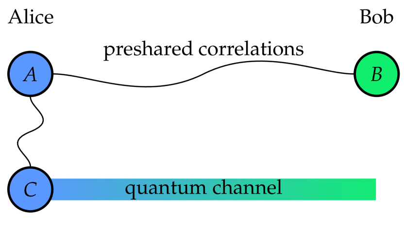
Figure 2: Indirect entanglement distribution. Alice and Bob initially share the state $\rho=\rho^{ABC}$, where Alice holds the particles $A$ and $C$, and Bob holds the particle $B$. Entanglement distribution is achieved by sending the particle $C$ from Alice to Bob via a (possibly noisy) quantum channel. The figure is taken from Streltsov et al. (2015a).

In the following discussion we will distinguish between direct and indirect entanglement distribution between two parties (Alice and Bob) Streltsov et al. (2015a); Zuppardo et al. (2016). Direct entanglement distribution is achieved if Alice prepares two particles in an entangled state $\rho$ and sends one of them to Bob. The amount of distributed entanglement is then given by $\mathcal{E}(\openone\otimes\Lambda[\rho])$, where $\Lambda$ describes the corresponding quantum channel, and $\mathcal{E}$ is a suitable entanglement measure.

Indirect entanglement distribution is a more general scenario where Alice and Bob already share correlations initially. In this case the total initial state is a tripartite state $\rho=\rho^{ABC}$, where Alice is in possession of the particles $A$ and $C$, and the particle $B$ is in Bob’s hands. Entanglement distribution is then achieved by sending the particle $C$ from Alice to Bob, see Fig. 2. The amount of distributed entanglement is then given by $\mathcal{E}^{A|BC}(\openone^{AB}\otimes\Lambda_{C}[\rho])-\mathcal{E}^{AC|B}(\rho)$. In the following, we will discuss recent results on these two types of entanglement distribution Streltsov et al. (2015a); Zuppardo et al. (2016).

IV.1 Direct entanglement distribution

What is the maximal amount of entanglement that can be directly distributed via a given quantum channel $\Lambda$? For answering this question, we first introduce the corresponding figure of merit:

$$\mathcal{E}_{\mathrm{direct}}(\Lambda)=\sup_{\sigma}\mathcal{E}\left(\openone\otimes\Lambda[\sigma]\right).$$ (22)

In general, the supremum is performed over all bipartite quantum states $\sigma$. However, if the entanglement quantifier $\mathcal{E}$ is convex, we can restrict ourselves to pure states.

If the distribution channel is noiseless, i.e., $\Lambda=\openone$, then Eq. (22) reduces to

$$\mathcal{E}_{\mathrm{direct}}(\openone)=\mathcal{E}(\phi_{d}^{+}),$$ (23)

where $d$ is the dimension of the carrier particle. It is tempting to believe that this also extends to noisy channels, i.e., that for any noisy channel the optimal performance is achieved by sending one half of a maximally entangled state. Quite surprisingly, this procedure is not optimal in general Ziman and Bužek (2007); Pal et al. (2014); Streltsov et al. (2015a). In particular, for any convex entanglement measure $\mathcal{E}$ there exists a noisy channel $\Lambda$ and a bipartite state $\rho$ such that Ziman and Bužek (2007)

$$\mathcal{E}(\openone\otimes\Lambda[\rho])>\mathcal{E}(\openone\otimes\Lambda[\phi_{d}^{+}]).$$ (24)

Even more, if entanglement is quantified via the logarithmic negativity, then states with arbitrary little entanglement can outperform maximally entangled states for some noisy channels Streltsov et al. (2015a). Nevertheless, maximally entangled states are still optimal in various scenarios, e.g. if the carrier particle is a qubit and entanglement quantifier is the entanglement of formation or the geometric entanglement Streltsov et al. (2015a). If the distribution channel is a single-qubit Pauli channel, i.e.,

$$\Lambda_{\mathrm{p}}[\rho]=\sum_{i=0}^{3}p_{i}\sigma_{i}\rho\sigma_{i},$$ (25)

where $\sigma_{i}$ are Pauli matrices with $\sigma_{0}=\openone$, then maximally entangled states are optimal for entanglement distribution, regardless of the particular entanglement measure Streltsov et al. (2015a):

$$\mathcal{E}_{\mathrm{direct}}(\Lambda_{\mathrm{p}})=\mathcal{E}(\openone\otimes\Lambda_{\mathrm{p}}[\phi_{2}^{+}]).$$ (26)

This result also holds if entanglement distribution is performed via a combination of (possibly different) Pauli channels, also in this case sending one half of a maximally entangled state is the best strategy. Finally, if entanglement is quantified via the logarithmic negativity, maximally entangled states are optimal for all unital single-qubit channels .

This completes our discussion on direct entanglement distribution, and we will present the more general scenario in the following.

IV.2 Indirect entanglement distribution

Can Alice and Bob gain an advantage if they share some correlations initially? To answer this question, we first introduce a figure of merit for indirect entanglement distribution:

$$\mathcal{E}_{\mathrm{indirect}}(\Lambda)=\sup_{\rho}\left\{\mathcal{E}^{A|BC}(\openone^{AB}\otimes\Lambda_{C}[\rho])-\mathcal{E}^{AC|B}(\rho)\right\},$$ (27)

where the supremum is taken over all tripartite states $\rho=\rho^{ABC}$. In particular, we are interested in the question if $\mathcal{E}_{\mathrm{indirect}}$ is larger than $\mathcal{E}_{\mathrm{direct}}$ for some noisy channel and some entanglement measure.

Note that so far no general answer to this question is known, and partial results have been presented in Streltsov et al. (2015a); Zuppardo et al. (2016). In particular, if the channel used for entanglement distribution is a single-qubit Pauli channel given in Eq. (25) and entanglement is quantified via a subadditive measure $\mathcal{E}$, then indirect entanglement distribution does not provide any advantage Streltsov et al. (2015a):

$$\mathcal{E}_{\mathrm{indirect}}(\Lambda_{\mathrm{p}})=\mathcal{E}_{\mathrm{direct}}(\Lambda_{\mathrm{p}})=\mathcal{E}(\openone\otimes\Lambda_{\mathrm{p}}[\phi_{2}^{+}]).$$ (28)

This means that in this case sending one half of a singlet state is the optimal distribution strategy. This result can be generalized to the case where entanglement is distributed via a combination of (possibly different) Pauli channels Streltsov et al. (2015a).

However, not all entanglement measures are subadditive. An important example is the distillable entanglement $\mathcal{E}_{\mathrm{d}}$ which was defined in Eq. (8) and is conjectured Shor et al. (2001) to violate subadditivity. Interestingly, if this conjecture is true, then indirect entanglement distribution provides an advantage for the distribution of distillable entanglement Streltsov et al. (2015a).

Finally, we note that entanglement breaking channels cannot be used for entanglement distribution for any entanglement measure $\mathcal{E}$ Zuppardo et al. (2016):

$$\mathcal{E}_{\mathrm{indirect}}(\Lambda_{\mathrm{eb}})=\mathcal{E}_{\mathrm{direct}}(\Lambda_{\mathrm{eb}})=0$$ (29)

for any entanglement breaking channel $\Lambda_{\mathrm{eb}}$. This can be seen by noting that any entanglement breaking channel is equivalent to an LOCC protocol Horodecki et al. (2003).

IV.3 Entanglement distribution with separable states

Entanglement can also be distributed by sending a carrier particle which is not entangled with the rest of the system. In particular, there exist tripartite states $\rho=\rho^{ABC}$ such that

$$\mathcal{E}^{AC|B}(\rho)=\mathcal{E}^{AB|C}(\rho)=0, \mathcal{E}^{A|BC}(\rho)>0.$$ (30)

The first example for a state fulfilling Eqs. (30) was presented in Cubitt et al. (2003), and can be written as

$$\eta=\frac{1}{3}\ket{\Psi_{\mathrm{GHZ}}}\!\bra{\Psi_{\mathrm{GHZ}}}+\sum_{i,j,k=0}^{1}\beta_{ijk}\Pi_{ijk},$$ (31)

with $\ket{\Psi_{\mathrm{GHZ}}}=(\ket{000}+\ket{111})/\sqrt{2}$, $\Pi_{ijk}=\ket{ijk}\!\bra{ijk}$, and all $\beta_{ijk}$ are zero apart from $\beta_{001}=\beta_{010}=\beta_{101}=\beta_{110}=1/6$. These results were extended to Gaussian states in Mišta and Korolkova (2008), and experiments verifying this phenomenon have also been reported Fedrizzi et al. (2013); Vollmer et al. (2013); Peuntinger et al. (2013).

Motivated by this result, Zuppardo et al. Zuppardo et al. (2016) proposed a classification of entanglement distribution protocols. In particular, a noiseless distribution protocol is called excessive if the amount of distributed entanglement is larger than the amount of entanglement between the carrier and the rest of the system, i.e.,

$$\mathcal{E}^{A|BC}(\rho)-\mathcal{E}^{AC|B}(\rho)>\mathcal{E}^{AB|C}(\rho).$$ (32)

Otherwise, the protocol is called nonexcessive. As discussed above, the state $\eta$ in Eq. (31) gives rise to an excessive distribution protocol.

It is natural to ask if such entanglement distribution with separable states can provide an advantage when compared to scenarios where the carrier particle is entangled with the rest of the system. In particular, one might ask if a separable state can show a better performance for entanglement distribution when compared to maximally entangled states. This question could be especially relevant if the distribution channel is noisy. Despite attempts by several authors Kay (2012); Fedrizzi et al. (2013), the question has not yet been settled.

Finally, we mention that rank two separable states are not useful for entanglement distribution if entanglement is quantified via logarithmic negativity Streltsov et al. (2014).

IV.4 Role of quantum discord for entanglement distribution

As was shown in Streltsov et al. (2012a); Chuan et al. (2012), the amount of entanglement that can be distributed via a noiseless channel by using a tripartite quantum state $\rho=\rho^{ABC}$ is bounded above by the discord between the carrier particle $C$ and the rest of the system:

$$\mathcal{E}^{A|BC}(\rho)-\mathcal{E}^{AC|B}(\rho)\leq\mathcal{D}^{C|AB}(\rho).$$ (33)

This inequality is true for any distance-based measure of entanglement and discord given in Eqs. (10) and (20) if the corresponding distance does not increase under quantum operations and fulfills the triangle inequality. Moreover, it is also true for the relative entropy of entanglement and discord Streltsov et al. (2012a); Chuan et al. (2012).

The inequality (33) immediately implies that zero-discord states cannot be used for entanglement distribution. Moreover, this result can also be used to bound the amount of entanglement in one cut of a tripartite state $\rho=\rho^{ABC}$ in terms of entanglement and discord in the other cuts Streltsov et al. (2012a); Chuan et al. (2012):

$$\mathcal{E}^{AC|B}(\rho)+\mathcal{D}^{C|AB}(\rho)\geq\mathcal{E}^{A|BC}(\rho)\geq\mathcal{E}^{AC|B}(\rho)-\mathcal{D}^{C|AB}(\rho).$$ (34)

For the relative entropy of entanglement and discord, the inequality (33) is saturated for pure states of the form $\ket{\psi}^{AC}\otimes\ket{\phi}^{B}$ and also for the state $\eta$ given in Eq. (31) Streltsov et al. (2012a).

If the channel used for entanglement distribution is noisy, we get the following generalized inequality Streltsov et al. (2015a):

$$\mathcal{E}^{A|BC}(\rho^{\prime})-\mathcal{E}^{AC|B}(\rho) \leq\min\left\{\mathcal{D}^{C|AB}(\rho),\mathcal{D}^{C|AB}(\rho^{\prime})\right\}.$$ (35)

Here, we used the notation $\rho^{\prime}=\openone^{AB}\otimes\Lambda_{C}[\rho]$, and $\mathcal{E}$ and $\mathcal{D}$ are any measures of entanglement and discord which fulfill Eq. (33).

V Conclusions

In this lecture we discussed recent results on entanglement distribution and the role of quantum discord in this task. Despite substantial progress in recent years, several important questions in this research field still remain open. In particular, it is still unclear if indirect entanglement distribution can provide an advantage in comparison to direct distribution protocols. The question also concerns entanglement distribution with separable states: also in this case it remains unclear if such scheme can be more useful than any direct distribution procedure.

We also mention that studying entanglement distribution in relation to the resource theory of coherence Baumgratz et al. (2014); Winter and Yang (2016); Streltsov et al. (2016) and its extension to distributed scenarios Bromley et al. (2015); Streltsov et al. (2015c); Chitambar et al. (2016); Ma et al. (2016); Chitambar and Hsieh (2016); Matera et al. (2016); Streltsov et al. (2015); Yadin et al. (2015) could potentially shed new light on these questions, and also lead to new independent results.