On the structure and statistical theory of turbulence of extended magnetohydrodynamics

Abstract

Recent progress regarding the noncanonical Hamiltonian formulation of extended magnetohydrodynamics (XMHD), a model with Hall drift and electron inertia, is summarized. The advantages of the Hamiltonian approach are invoked to study some general properties of XMHD turbulence, and to compare them against their ideal MHD counterparts. For instance, the helicity flux transfer rates for XMHD are computed, and Liouville’s theorem for this model is also verified. The latter is used, in conjunction with the absolute equilibrium states, to arrive at the spectra for the invariants, and to determine the direction of the cascades, e.g., generalizations of the well-known ideal MHD inverse cascade of magnetic helicity. After a similar analysis is conducted for XMHD by inspecting second order structure functions and absolute equilibrium states, a couple of interesting results emerge. When cross helicity is taken to be ignorable, the inverse cascade of injected magnetic helicity also occurs in the Hall MHD range - this is shown to be consistent with previous results in the literature. In contrast, in the inertial MHD range, viz.  at scales smaller than the electron skin depth, all spectral quantities are expected to undergo direct cascading. The consequences and relevance of our results in space and astrophysical plasmas are also briefly discussed.

I Introduction

In most areas of fusion, space and astrophysical plasmas, fluid models have proven to be highly useful in capturing the relevant physics (Dungey, 1958; Krall and Trivelpiece, 1973; Goedbloed and Poedts, 2004; Freidberg, 2014). Amongst them, the simplest and most widely used is ideal magnetohydrodynamics (MHD). Although MHD has proven to be very successful in predicting many phenomena, it is known to be valid only in certain regimes. There exist a wide class of systems, particularly in astrophysics and space science, which are collisionless with non-ideal MHD effects becoming important. For instance, one such notable contribution is the Hall effect that becomes non-negligible when the characteristic frequencies become comparable to, or greater than, the ion cyclotron frequency $\omega_{ci}$ (Bellan, 2008). Another crucial effect worth highlighting is due to electron inertia, which becomes important when one considers characteristic length scales that are smaller than the electron skin depth $d_{e}=c/\omega_{pe}$ with $\omega_{pe}$ denoting the electron plasma frequency.

Thus, it is advantageous to seek fluid models containing the above two effects. Extended MHD, henceforth referred to as XMHD, is a model that is endowed with both the Hall drift and electron inertia (Lüst, 1959). It can be rigorously derived from two-fluid theory through a series of systematic orderings and expansions, as shown in Dungey (1958); Goedbloed and Poedts (2004); Keramidas Charidakos et al. (2014). Although it has long since been known that ideal MHD has both action principle (Newcomb, 1962) and Hamiltonian (Morrison and Greene, 1980) formulations, the XMHD equivalents proved to be quite elusive until recently - the former was presented in Keramidas Charidakos et al. (2014); D’Avignon et al. (2016) and the latter in Abdelhamid et al. (2015); Lingam et al. (2015a). At this stage, it is important and instructive to pose two crucial questions. What general benefits do the Hamiltonian and Action Principle (HAP) formulations accord? Secondly, what are the physical systems and phenomena where extended MHD has been successfully employed?

The first question has already been explored extensively, and we refer the reader to the reviews by Serrin (1959); Morrison (1982); Zakharov et al. (1985); Holm et al. (1985); Salmon (1988); Zakharov et al. (1992); Morrison (1998, 2005). Some of the chief advantages, apart from their inherent mathematical elegance and simplification, include:

• A systematic and rigorous means of constructing equilibria and obtaining sufficient conditions for their stability (Holm et al., 1985). This was recently applied to ideal MHD in a series of works by Andreussi et al. (2013, 2016); see also Morrison et al. (2013).

• A clear derivation of reduced models without the loss of the Hamiltonian nature, and thereby avoiding ‘spurious’ dissipation; for e.g., Morrison and Hazeltine (1984); Hazeltine et al. (1987); Morrison et al. (2014); Lingam (2015); Keramidas Charidakos et al. (2015).

• The extraction of important invariants such as the magnetic helicity and its generalizations (Calkin, 1963; Holm et al., 1985; Padhye and Morrison, 1996; Lingam et al., 2016). This is done by means of the particle relabelling symmetry (Padhye and Morrison, 1996) in the action principle approach and via the degeneracy of the noncanonical Poisson bracket in the Hamiltonian formulation (Yoshida et al., 2014). It is also possible to establish and elucidate topological properties of XMHD by means of the HAP approach, as recently shown in D’Avignon et al. (2016); Lingam et al. (2016).

• A detailed understanding of how magnetic reconnection operates by taking advantage of the underlying Hamiltonian structure, such as the aforementioned invariants (Ottaviani and Porcelli, 1993; Cafaro et al., 1998; Grasso et al., 2001; Tassi et al., 2008; Comisso et al., 2012, 2013; Hirota et al., 2015).

• A natural means of arriving at weak turbulence theories, as described in Zakharov et al. (1992); Zakharov and Kuznetsov (1997); Nazarenko (2011). This methodology was applied to Hall MHD by Sahraoui et al. (2003). The reader is directed to the analysis by Abdelhamid et al. (2016) that drew extensively upon the HAP approach (for e.g., to construct nonlinear wave solutions), and thereby arrived at the energy and helicity spectra of XMHD. We also point out the recent beatification procedure of Viscondi et al. (2016) as an elegant alternative, that explicitly relies on the Hamiltonian formulation.

• The knowledge of the HAP structures has proven to be highly useful numerically for constructing structure preserving integrators (variational and symplectic) (Candy and Rozmus, 1991; Qin and Guan, 2008; Evstatiev and Shadwick, 2013; Ellison et al., 2015; Tronko et al., 2016; Kraus et al., 2016). These integrators have (definitively) outperformed other conventional choices, as the latter lack the unique conservation laws and geometric properties of the former.

In addition to these (admittedly representative) benefits, we also observe that the HAP approach has been tangentially employed in astrophysical phenomena such as Hall MHD dynamos (Mininni et al., 2003; Lingam and Bhattacharjee, 2016a, b) and jets (Lingam and Mahajan, 2015). Thus, it is quite evident that a thorough understanding of the Hamiltonian and Action Principle (HAP) formalisms for XMHD is quite warranted. However, this brings us to the second point, concerning the physical relevance and importance of the model (XMHD) itself.

Fortunately, there are several instances where XMHD has proven to be a very useful physical model. From the perspective of fundamental plasma phenomena, both turbulence and reconnection results have been radically altered since the Hall term (and electron inertia) was taken into account. In the case of the latter field in particular, it is not an exaggeration to say that the whole field was revitalized through the inclusion of this one simple term. The reader may consult the excellent texts by Biskamp (2000); Birn and Priest (2007) on this subject. In turbulence, it has been shown that the introduction of Hall drift (and electron inertia) leads to the steepening of spectra (Krishan and Mahajan, 2004; Galtier, 2006; Galtier and Buchlin, 2007; Shaikh and Shukla, 2009; Abdelhamid et al., 2016). Each of these theoretical consequences has been confirmed through detailed observations of the Earth’s magnetosphere (Kivelson and Russell, 1995; Burch et al., 2016), and the solar wind and corona (Sahraoui et al., 2009; Parnell and De Moortel, 2012; Bruno and Carbone, 2013; Sahraoui et al., 2013; Alexandrova et al., 2013; Narita et al., 2016). Lastly, we also wish to note that certain fusion phenomena, such as sawtooth crashes (Hastie, 1997), have also been explained well by utilizing XMHD.

The outline of our paper is as follows. In Sec. II, we discuss the noncanonical Hamiltonian structure of XMHD, and some of its salient features. We follow this up by using some of these aspects to gain a better understanding XMHD turbulence. In Sec. III, we generalize the results of Banerjee and Galtier (2016) on helicity flux transfer rates to include electron inertia, and we also briefly raise the issue of the directional nature of the cascades. This matter is addressed in more detail in Sec. IV, where we predict that the inverse cascade of magnetic helicity operates in the Hall MHD regime, but is absent when we consider the inertial MHD range that is valid at sub-electron skin depth scales. Finally, we conclude with a summary of our results and their implications in Sec. V.

II The Hamiltonian formulation of extended MHD

In the present section, we introduce the equations of the extended MHD model, and discuss its Hamiltonian structure as well as the insights that follow as a natural consequence.

II.1 Preliminary model considerations

Although the correct form of the equations of XMHD has been known since the 1950s (Dungey, 1958; Lüst, 1959), many different variants exist in the literature. Of these, it is worth remarking that some of them are incorrect and do not conserve energy (Kimura and Morrison, 2014).

The XMHD equations comprise of the continuity equation, the momentum equation and the generalized Ohm’s law (Goedbloed and Poedts, 2004; Birn and Priest, 2007). They are respectively given by

$$\frac{\partial\rho}{\partial t}+\nabla\cdot\left(\rho{\bf V}\right)=0,$$ (1)

$$\rho\left(\frac{\partial{\bf V}}{\partial t}+{\bf V}\cdot\nabla{\bf V}\right)=-\nabla p+{\bf J}\times{\bf B}\,-\frac{m_{e}}{e^{2}}{\bf J}\cdot\nabla\left(\frac{{\bf J}}{n}\right),$$ (2)

$${\bf E}+{\bf V}\times{\bf B}-\frac{{\bf J}\times{\bf B}-\nabla p_{e}+\mu\nabla p_{i}}{en}=\frac{m_{e}}{ne^{2}}\left[\frac{\partial{\bf J}}{\partial t}+\nabla\cdot\left({\bf V}{\bf J}+{\bf J}{\bf V}-\frac{1}{en}{\bf J}{\bf J}\right)\right].$$ (3)

Here, note that the one-fluid variables $\rho$, ${\bf V}$ and ${\bf J}=\mu_{0}^{-1}\nabla\times{\bf B}$ are the total mass density, the centre-of-mass velocity and the current respectively. ${\bf E}$ and ${\bf B}$ denote the electric and magnetic fields, whilst $p_{s}$ is the pressure of species ‘$s$’ and $p=p_{i}+p_{e}$ is the total pressure. The variables $m_{e}$ and $e$ are the electron mass and charge, whilst $\mu=m_{e}/m_{i}$ is the mass ratio. An inspection of (3) reveals that it is far more complex than the ideal MHD Ohm’s law that follows by setting all terms except the first two (on the LHS) to zero.

The next step is to render the above equations dimensionless. This is done by normalizing everything in terms of Alfvénic units, and the reader is directed to Abdelhamid et al. (2015); Lingam et al. (2016) for further details. We also introduce the dynamical variable

$${\bf B}^{*}={\bf B}+d_{e}^{2}\,\nabla\times\left[\frac{\nabla\times{\bf B}}{\rho}\right],$$ (4)

which is well known from previous theories that relied upon electron inertia, such as Ottaviani and Porcelli (1993); Cafaro et al. (1998). After some algebraic manipulation (2) and (3) can be expressed in a simpler manner as follows.

$$\frac{\partial{\bf V}}{\partial t}+\left(\nabla\times{\bf V}\right)\times{\bf V}=-\nabla\left(h+\frac{V^{2}}{2}\right)+\frac{\left(\nabla\times{\bf B}\right)\times{\bf B}^{*}}{\rho}-d_{e}^{2}\nabla\left[\frac{\left(\nabla\times{\bf B}\right)^{2}}{2\rho^{2}}\right],$$ (5)

$$\frac{\partial{\bf B}^{*}}{\partial t}=\nabla\times\left({\bf V}\times{\bf B}^{*}\right)-d_{i}\nabla\times\left(\frac{\left(\nabla\times{\bf B}\right)\times{\bf B}^{*}}{\rho}\right)+d_{e}^{2}\nabla\times\left[\frac{\left(\nabla\times{\bf B}\right)\times\left(\nabla\times{\bf V}\right)}{\rho}\right].$$ (6)

In obtaining the above two equations, we observe that a barotropic pressure was implicitly assumed; for a non-barotropic treatment, we refer the reader to Keramidas Charidakos et al. (2014); D’Avignon et al. (2016). In the above expressions, note that $d_{s}=c/(\omega_{ps}L)$ is the skin depth of species ‘$s$’ normalized to the characteristic length scale $L$, and $\omega_{ps}$ is the corresponding plasma frequency. All of these values are in terms of the fiducial units that were adopted for the purpose of normalization.

II.2 The Hamiltonian structure of extended MHD

We are now in a position to present the Hamiltonian formulation of extended MHD. A detailed derivation of this structure can be found in Abdelhamid et al. (2015); Lingam et al. (2015a); D’Avignon et al. (2016) and a recent overview was provided in Lingam et al. (2016).

Firstly, we observe that (1), (5) and (6) can be used to show that the following energy functional is conserved.

$$H=\int_{D}d^{3}x\,\left[\frac{\rho V^{2}}{2}+\rho U(\rho)+\frac{B^{2}}{2}+d_{e}^{2}\frac{\left(\nabla\times{\bf B}\right)^{2}}{2\rho}\right],$$ (7)

where $D\subset\mathbb{R}^{3}$ (Morrison, 1982). It is worth remarking that there is no $d_{i}$ dependence, but there is a $d_{e}$-dependent term, which stems from the electron fluid velocity. Upon setting $d_{e}\rightarrow 0$, we will obtain the famous ideal MHD energy (Newcomb, 1962).

From basic classical mechanics, we know that a system can be rendered Hamiltonian if one has a conserved “energy” and a suitable Poisson bracket. The Poisson bracket must satisfy the properties of (i) bilinearity, (ii) antisymmetry, (iii) the Leibniz product rule, and (iv) the Jacobi identity (Sudarshan and Mukunda, 2016). Even though our Poisson bracket is infinite-dimensional (and degenerate), it must still satisfy these properties.

It is instructive to first begin with Hall MHD (HMHD), which is the best known of all the extended magnetofluid models. As noted earlier, it has proven to be highly useful in explaining phenomena such as magnetic reconnection, dynamos, and turbulence. The correct noncanonical Poisson bracket was provided by Yoshida and Hameiri (2013), and is given by

$$\{F,G\}^{HMHD} = -\int_{D}d^{3}x\,\Bigg{\{}\left[F_{\rho}\nabla\cdot G_{\bf V}+F_{\bf V}\cdot\nabla G_{\rho}\right]-\frac{\left(\nabla\times{\bf V}\right)}{\rho}\cdot\left(F_{\bf V}\times G_{\bf V}\right)$$

$$\hskip 50.58878pt-\frac{{\bf B}}{\rho}\cdot\left(F_{\bf V}\times\left(\nabla\times G_{\bf B}\right)\right)+\frac{{\bf B}}{\rho}\cdot\left(G_{\bf V}\times\left(\nabla\times F_{\bf B}\right)\right)\Bigg{\}}$$

$$-\,d_{i}\int_{D}d^{3}x\,\frac{{\bf B}}{\rho}\cdot\left[\left(\nabla\times F_{\bf B}\right)\times\left(\nabla\times G_{\bf B}\right)\right],$$

where $F_{\phi}:=\delta F/\delta\phi$ is the functional derivative (Morrison, 1982) with respect to $\phi$. It is more transparent to write the above equation as

$$\{F,G\}^{HMHD}=\{F,G\}^{MHD}+\{F,G\}^{Hall},$$ (8)

where the first two lines of (II.2) constitute the classic MHD bracket $\{F,G\}^{MHD}$ that was first derived by Morrison and Greene (1980). The last line of (II.2), with the factor of $d_{i}$ in front, gives rise to the Hall contributions in the Ohm’s law.

Next, let us turn our attention to (3) once more. The Hall MHD Ohm’s law follows by setting everything on the RHS alone to zero. Instead, suppose we consider a case where the third term, with a factor of $en$ in the denominator, is set to zero. In our choice of normalized units, this amounts to setting $d_{i}\rightarrow 0$ but not $d_{e}\rightarrow 0$ as well. This may appear counterintuitive, but we observe that $d_{i}$ and $d_{e}$ must be perceived as independent variables. The resultant model has sometimes been referred to as inertial MHD (Kimura and Morrison, 2014; Lingam et al., 2015b), because it encompasses electron inertia but not the Hall term.

Although inertial MHD (IMHD) may appear somewhat ad hoc at this stage, it can be derived through a rigorous ordering procedure as discussed in Kimura and Morrison (2014); Lingam et al. (2016). Moreover, it is particularly useful in deriving reduced models for reconnection (Ottaviani and Porcelli, 1993; Fitzpatrick and Porcelli, 2004, 2007). It has also proven to be useful in studying dynamo action (Kleva, 1994), as the inertial MHD Ohm’s law is linear in ${\bf B}$. In Lingam et al. (2015a, 2016), it was shown that a remarkable equivalence between the Hall and inertial MHD Poisson brackets exists. This equivalence can be expressed as

$$\{F,G\}^{IMHD}\equiv\{F,G\}^{HMHD}\left[\mp 2d_{e};\,\bm{\mathcal{B}}_{\pm}^{(I)}\right],$$ (9)

where the LHS is to be understood as follows. Replace ${\bf B}$ everywhere in the Hall MHD bracket (II.2) with $\bm{\mathcal{B}}_{\pm}^{(I)}:={\bf B}^{*}\pm d_{e}\nabla\times{\bf V}$ and $d_{i}$ with $\mp 2d_{e}$, where ${\bf B}^{*}$ was defined in (4). Owing to the presence of the ‘$\pm$’, it is clear that there are two such transformations which lead to the equivalence. In Sec. II.3, we shall comment on the nature of these transformations further.

Finally, let us consider extended MHD (XMHD) in its entirety, i.e., where no terms are dropped from the Ohm’s law (3). The noncanonical Poisson bracket for this model was derived by Abdelhamid et al. (2015), and Lingam et al. (2015a) showed that another beautiful equivalence between the Hall and extended MHD brackets existed. In mathematical terms, it amounts to

$$\{F,G\}^{XMHD}\equiv\{F,G\}^{HMHD}\left[d_{i}-2\kappa_{\pm};\,\bm{\mathcal{B}}_{\pm}\right],$$ (10)

where the RHS indicates that the substitutions

$${\bf B}\rightarrow\bm{\mathcal{B}}_{\pm}:={\bf B}^{*}+\kappa_{\pm}\nabla\times{\bf V},$$ (11)

and $d_{i}\rightarrow d_{i}-2\kappa_{\pm}$ in (II.2) lead to the XMHD bracket. Again, there are two such transformations since $\kappa_{\pm}$ follow from determining the two roots of the quadratic equation

$$\kappa^{2}-d_{i}\kappa-d_{e}^{2}=0.$$ (12)

Here, observe that setting $d_{i}=0$ leads us to the inertial-Hall MHD equivalence discussed above, and also transforms (11) to $\bm{\mathcal{B}}_{\pm}^{(I)}$.

Before proceeding further, a comment on why these connections between the different models are remarkable is in order. In Hall MHD, there is no electron inertia but there is a finite Hall drift. In inertial MHD, the situation is exactly reversed, i.e. there is no Hall drift but there is electron inertia. Thus, it is not at all intuitively obvious that the two models could share a common Hamiltonian structure, since their effects are mutually exclusive. Yet, the above relations show that there does exist a deep, and non-trivial, equivalence between the two models. This equivalence is also shared by extended MHD, which has both Hall drift and electron inertia. Here, it must be understood that the “equivalence” referred to thus far between Hall MHD and inertial MHD is only concerned with their respective Poisson brackets. The corresponding Hamiltonians for these two models are not identical, as they differ by a single term, i.e. the last one in (7).

Subsequently, we shall explore the different predictions regarding the behavior of turbulent cascades in Sections IV.3 and IV.4.

II.3 On the topological properties of extended MHD

We have seen earlier that the variable (11) lies at the heart of the equivalence between the different models. To understand why, it is instructive to take a step backwards and consider ideal MHD. In any introductory textbook, the frozen-flux property of ideal MHD and the conservation of magnetic helicity $\int_{D}d^{3}x\,{\bf A}\cdot{\bf B}$ are presented. Thus, it is natural to ask if one can seek generalizations of these properties to XMHD, since both of these features are present in two-fluid theory (Spencer and Kaufman, 1982; Steinhauer and Ishida, 1997) and in Hall MHD (Turner, 1986).

In ideal MHD, the frozen-flux constraint can be expressed as

$${\bf B}\cdot d{\bf S}={\bf B}^{0}\cdot d{\bf S}^{0},$$ (13)

where $d{\bf S}$ is the area element, and the superscript ‘$0$’ denotes the values at $t=0$ (Newcomb, 1962). It is also possible to view the above expression as the statement that the magnetic flux (in ideal MHD) is a Lie-dragged 2-form; for more details, the reader may consult Tur and Yanovsky (1993).

In XMHD, there are two such generalized frozen-flux constraints, given by

$$\bm{\mathcal{B}}_{\pm}\cdot d{\bf S}_{\pm}=\bm{\mathcal{B}}_{\pm}^{0}\cdot d{\bf S}^{0}_{\pm},$$ (14)

where $\bm{\mathcal{B}}_{\pm}$ was defined in (11) and $d{\bf S}_{\pm}$ denotes the corresponding area element. This elegant property was first recognized in Lingam et al. (2015a), later proven in Lingam et al. (2016) and utilized further in D’Avignon et al. (2016).

Next, let us consider the helicity. In ideal MHD, the magnetic helicity is conserved, but it is no ordinary invariant. Instead, it is both a Casimir invariant and a topological invariant. Casimir invariants are special invariants that follow from the degeneracy of the (noncanonical) Poisson bracket, and they are found via $\{F,C\}=0\,\,\forall\,F$, with $C$ denoting the Casimir invariant. They play an important role in regulating the phase space dynamics, as discussed in Morrison (1998), and have played an important role in reconnection over the years (Ottaviani and Porcelli, 1993; Cafaro et al., 1998; Grasso et al., 2001). Magnetic helicity is also a topological invariant since it is closely connected with the linking and twisting of field lines - more precisely, it shares close connections with the Gauss linking number as discussed in Moreau (1961); Moffatt (1969); Berger and Field (1984).

Thus, one can obtain the generalized counterparts of the magnetic helicity in extended MHD by seeking out the Casimir invariants that resemble it. There are two such invariants

$$\mathcal{K}_{\pm}=\int_{D}d^{3}x\,\bm{\mathcal{A}}_{\pm}\cdot\bm{\mathcal{B}}_{\pm},$$ (15)

where $\bm{\mathcal{B}}_{\pm}=\nabla\times\bm{\mathcal{A}}_{\pm}$, and the LHS is given by (11). It is clear that these generalized helicities have the same form of the magnetic and fluid helicities (for MHD and HD respectively), and hence one may expect them to share similar topological properties. This conjecture was confirmed in Lingam et al. (2016), where the authors also established some unusual connections with Chern-Simons theory, a ubiquitous (topological) quantum field theory that appears in high-energy and condensed matter physics.

From the preceding discussion, it is clear that the variable $\bm{\mathcal{B}}_{\pm}$ that facilitates the equivalence between the different extended magnetofluid models is not arbitrary. It has close connections with the generalized frozen-fluxes, helicities and Lie-dragged 2-forms all of which have clear mathematical and physical significance. Lastly, it is also possible to manipulate (5) and (6) directly to arrive at

$$\partial_{t}\bm{\mathcal{A}}_{\pm}=\mathbf{V}_{\pm}\times\bm{\mathcal{B}}_{\pm}+\nabla\psi_{\pm}\quad\text{and}\quad\partial_{t}\bm{\mathcal{B}}_{\pm}=\nabla\times(\mathbf{V}_{\pm}\times\bm{\mathcal{B}}_{\pm}),$$ (16)

where $\mathbf{V}_{\pm}:=\bm{V}-\kappa_{\mp}\nabla\times\bm{B}$ and

$$\psi_{\pm}:=\kappa_{\mp}h_{e}-\Big{(}\kappa_{\pm}+\frac{d_{e}^{2}}{d_{i}}\Big{)}h_{i}-\phi+\kappa_{\mp}d_{e}^{2}\,\frac{J^{2}}{2\rho}-d_{e}^{2}\frac{\mathbf{J}\cdot\mathbf{V}}{\rho},$$ (17)

as shown in Lingam et al. (2016). Upon inspection, it is clear that the second set of equations in (16) exactly resemble the induction equation in ideal MHD, thereby emphasizing the role of $\bm{\mathcal{B}}_{\pm}$ as the generalization of the magnetic field. It is, however, more common to refer to it as the generalized (or canonical) vorticity.

Thus, to summarize our discussion up to this point, we have seen that the Hamiltonian formulation of XMHD has led us to two important conclusions.

• There exists a high degree of mathematical similarity between the different models, even though they have contrasting (and sometimes exclusive) physical effects. This mathematical equivalence between the models is rendered very clear when written in Hamiltonian form. Hence, the latter approach serves as a means of unifying the different extended MHD models.

• The similarities between extended MHD and ideal MHD can be understood further by means of the HAP formulations, which lead us to the generalizations of the helicity, flux, and induction equation.

Bearing these advantages in mind, we shall now proceed to study some pertinent features of XMHD turbulence in the subsequent sections.

III Flux transfer rates

In the recent work by Banerjee and Galtier (2016), expressions for the dissipation rates for Hall MHD were computed. Their analysis assumed that the Hall MHD turbulence was homogeneous, but did not rely on the further assumption of isotropy. As noted above, an important limitation of Hall MHD is that it becomes invalid when electron inertia effects start to dominate, i.e.  when one considers length scales comparable to the electron skin depth. In such an instance, it makes sense to use extended MHD instead, on account of the fact that it is endowed with electron inertia effects.

In recent times, there has also been a great deal of interest focused on the solar wind at sub-electron scales, mostly because of the fact that observations have now become possible in this regime (Sahraoui et al., 2009; Alexandrova et al., 2009; Sahraoui et al., 2011; Bruno and Carbone, 2013; Sahraoui et al., 2013). Hence, in the present section, we shall generalize the results of Banerjee and Galtier (2016) by including electron inertia.

III.1 Mean helicity flux rates

In 3D fluid turbulence, it has been known since the famous works by Kolmogorov (1941), and subsequent numerical and experimental tests (Frisch, 1995; Sreenivasan and Antonia, 1997; Biskamp, 2003), that the energy input at large scales flows to small dissipative scales. This phenomenon is often referred to as a direct Kolmogorov-Richardson cascade (Frisch, 1995) - a pictorial description of this phenomenon has been provided in Fig. 1.

Figure 1: Schematics of the standard Richardson-Kolmogorov direct cascade. Energy injected at low $k$, e.g.  via large scale stirring, cascades through the inertial range and dissipates at small scales (large $k$). Upon reversal of the arrows along with the driving and dissipative ranges, the mechanism of the inverse cascade is obtained.

In MHD, the direct cascade of energy and the inverse cascade of magnetic helicity (Frisch et al., 1975) have been widely explored, and are thus well established (Biskamp, 2003). In the inertial range, it must be borne in mind that the dissipation does not play a role. Hence, it is expected that, in the stationary regime, the same flux (of the energy or helicity, for example) flows through each wave number $k$. This principle was recently employed to conduct a complementary study of XMHD turbulence in Abdelhamid et al. (2016).

In our analysis, we are interested in the flux rate of the generalized helicities (15) within the framework of XMHD that are injected at some length scale. By following the steps outlined in Banerjee and Galtier (2016), we first introduce the symmetric two-point correlation function

$$R_{\mathcal{K}_{\pm}}=R_{\mathcal{K}_{\pm}}^{\prime}=\Bigg{\langle}\frac{\bm{\mathcal{A}}^{\prime}_{\pm}\cdot\bm{\mathcal{B}}_{\pm}+\bm{\mathcal{A}}_{\pm}\cdot\bm{\mathcal{B}}^{\prime}_{\pm}}{2}\Bigg{\rangle},$$ (18)

where primed quantities are functions of $\mathbf{x}^{\prime}=\mathbf{x}+\mathbf{r}$, unprimed quantities depend on $\mathbf{x}$, and the brackets $\langle\ \rangle$ are a shorthand notation for ensemble averaging. When the turbulence is homogeneous this can be equivalent to the spatial average. Upon manipulation we find

$$\partial_{t}\big{\langle}\bm{\mathcal{A}}^{\prime}_{\pm}\cdot\bm{\mathcal{B}}_{\pm}+\bm{\mathcal{A}}_{\pm}\cdot\bm{\mathcal{B}}^{\prime}_{\pm}\big{\rangle}=\big{\langle}\nabla\cdot[(\mathbf{V}_{\pm}\times\bm{\mathcal{B}}_{\pm})\times\bm{\mathcal{A}}^{\prime}_{\pm}]+\nabla^{\prime}\cdot[(\mathbf{V}_{\pm}^{\prime}\times\bm{\mathcal{B}}_{\pm}^{\prime})\times\bm{\mathcal{A}}_{\pm}]$$

$$\hskip 56.9055pt+\ \mathbf{V}_{\pm}^{\prime}\times\bm{\mathcal{B}}_{\pm}^{\prime}\cdot\bm{\mathcal{B}}_{\pm}+\mathbf{V}_{\pm}\times\bm{\mathcal{B}}_{\pm}\cdot\bm{\mathcal{B}}_{\pm}^{\prime}+\nabla\psi_{\pm}\cdot\bm{\mathcal{B}}_{\pm}^{\prime}+\nabla^{\prime}\psi_{\pm}^{\prime}\cdot\bm{\mathcal{B}}_{\pm}\big{\rangle}\,.$$ (19)

At this stage, we shall digress a little to explain how the principle of statistical homogeneity can be gainfully employed. Our discussion mirrors the one presented in George (2013). We introduce the change-of-variables $\bm{\xi}=\mathbf{x}^{\prime}+\mathbf{x}$ and $\mathbf{r}=\mathbf{x}^{\prime}-\mathbf{x}$, which implies that $\partial/\partial\mathbf{x}=\partial/\partial\bm{\xi}-\partial/\partial\bm{r}$ and $\partial/\partial\mathbf{x}^{\prime}=\partial/\partial\bm{\xi}+\partial/\partial\mathbf{r}$. For a given vector field ${\bf u}$, this implies that

$$\Big{\langle}u_{j}(\mathbf{x}^{\prime},t)\frac{\partial u_{i}(\mathbf{x},t)}{\partial x_{i}}\Big{\rangle} = \frac{\partial}{\partial x_{i}}\langle u_{j}(\mathbf{x}^{\prime},t)\,u_{i}(\mathbf{x},t)\rangle=-\frac{\partial}{\partial r_{i}}\langle u_{j}(\mathbf{x}^{\prime},t)\,u_{i}(\mathbf{x},t)\rangle$$ (20)

$$= -\frac{\partial}{\partial x_{i}^{\prime}}\langle u_{j}(\mathbf{x}^{\prime},t)\,u_{i}(\mathbf{x},t)\rangle=-\Big{\langle}\frac{\partial u_{j}(\mathbf{x}^{\prime},t)}{\partial x_{i}^{\prime}}u_{i}(\mathbf{x},t)\Big{\rangle}\,.$$

Upon using the above identity in (III.1), we obtain

$$\big{\langle}\nabla\cdot[(\mathbf{V}_{\pm}\times\bm{\mathcal{B}}_{\pm})\times\bm{\mathcal{A}}^{\prime}_{\pm}]+\nabla^{\prime}\cdot[(\mathbf{V}_{\pm}^{\prime}\times\bm{\mathcal{B}}_{\pm}^{\prime})\times\bm{\mathcal{A}}_{\pm}]\big{\rangle}$$

$$\hskip 42.67912pt=-\,\big{\langle}\nabla^{\prime}\cdot[(\mathbf{V}_{\pm}\times\bm{\mathcal{B}}_{\pm})\times\bm{\mathcal{A}}^{\prime}_{\pm}]+\nabla\cdot[(\mathbf{V}_{\pm}^{\prime}\times\bm{\mathcal{B}}_{\pm}^{\prime})\times\bm{\mathcal{A}}_{\pm}]\big{\rangle}$$

$$\hskip 42.67912pt=\big{\langle}\mathbf{V}_{\pm}\times\bm{\mathcal{B}}_{\pm}\cdot\bm{\mathcal{B}}^{\prime}_{\pm}+\mathbf{V}_{\pm}^{\prime}\times\bm{\mathcal{B}}_{\pm}^{\prime}\cdot\bm{\mathcal{B}}_{\pm}\rangle=-\langle\delta(\mathbf{V_{\pm}\times\bm{\mathcal{B}}_{\pm}})\cdot\delta\bm{\mathcal{B}}_{\pm}\big{\rangle}\,,$$ (21)

where $\delta f:=f^{\prime}-f$. Likewise, it is possible to show that

$$\big{\langle}\nabla^{\prime}\psi^{\prime}_{\pm}\cdot\bm{\mathcal{B}}_{\pm}+\nabla\psi_{\pm}\cdot\bm{\mathcal{B}}_{\pm}^{\prime}\big{\rangle}=-\big{\langle}\psi^{\prime}_{\pm}\nabla\cdot\bm{\mathcal{B}}_{\pm}+\psi_{\pm}\nabla^{\prime}\cdot\bm{\mathcal{B}}_{\pm}^{\prime}\big{\rangle}=0.$$ (22)

Thus, upon combining everything together, we get

$$\frac{\partial}{\partial t}\Big{[}\frac{1}{2}\,\big{\langle}\bm{\mathcal{A}}^{\prime}_{\pm}\cdot\bm{\mathcal{B}}_{\pm}+\bm{\mathcal{A}}_{\pm}\cdot\bm{\mathcal{B}}^{\prime}_{\pm}\big{\rangle}\Big{]}=-\big{\langle}\delta(\mathbf{V_{\pm}\times\bm{\mathcal{B}}_{\pm}})\cdot\delta\bm{\mathcal{B}}_{\pm}\big{\rangle}+D\,,$$ (23)

where we have introduced the phenomenological damping $D$ that occurs at the sink scale, following the approach of Banerjee and Galtier (2016). In the limit of infinite kinetic and magnetic Reynolds numbers, under the assumption of stationarity, the LHS of the above expression vanishes due to the ruggedness of the helicity invariants (Matthaeus and Goldstein, 1982). Hence, the large scale dissipation equals the mean generalized helicity flux rate

$$\eta_{\pm}=\big{\langle}\delta(\mathbf{V_{\pm}\times\bm{\mathcal{B}}_{\pm}})\cdot\delta\bm{\mathcal{B}}_{\pm}\big{\rangle}\,,$$ (24)

which closely resembles the expression of Banerjee and Galtier (2016). However, it must be noted that our expression is more general as it duly encompasses electron inertial contributions as well via the definition of $\bm{\mathcal{B}}_{\pm}$. In the Hall MHD limit with $d_{e}\rightarrow 0$, we have verified that our result is in exact agreement with the expression of Banerjee and Galtier (2016).

Although (24) is quite compact, a great deal of information can be extracted from it. For instance, it follows that the dissipation rates vanish when the Beltrami condition $\bm{\mathcal{B}}_{\pm}\parallel\mathbf{V}_{\pm}$ is attained. These (multi) Beltrami states are non-trivial, as they are also equilibria of XMHD (Abdelhamid et al., 2016). This is easy to verify by inspecting the second set of equations in (16), and substituting the above condition. Thus, this result serves as a consistency check indicating that the dissipation vanishes when the system has settled into this equilibrium (in the limit of infinite Reynolds numbers).

In Banerjee and Galtier (2016) a phenomenological argument for the direction of the cascades was presented. First, let us recall that the generalized helicities become the magnetic and ion canonical helicities in Hall MHD (Turner, 1986). The first is essentially a copy of the MHD magnetic helicity, while the other is a superposition of MHD cross helicity and fluid helicity after some rearrangement. In the former, it is argued that the inverse cascade is expected just as in ideal MHD. In contrast, the direction of the cascade for the ion canonical helicity (of Hall MHD) can go either way, as it is dependent on the energy budget of the system. It is assumed to exhibit an inverse cascade if the magnetic energy is dominant over the kinetic (and thermal) energy.

Therefore, we see that there is an ambiguity regarding the directionality of the cascade for one of the helicities. The problem becomes far more acute when we include electron inertia effects via XMHD. In that case, the magnetic helicity is not conserved as there is also a (smaller) fluid helicity contribution. If we apply the above line of reasoning, we would expect to witness the direct and inverse cascades of both helicities in XMHD. This is because of the fact that the two helicities are not fundamentally different, other than the fact that they are associated with different species (Lingam et al., 2015a, 2016). Thus, this raises an interesting question: how is it possible to get the Hall MHD limit from XMHD? In other words, why is the direct cascade of one helicity, that corresponds to the magnetic helicity in the HMHD limit, lost? One possible resolution of this paradox is by suggesting that the existence of direct or inverse cascades depends on the length scale we are considering. This question is addressed in more detail in Sec. IV that follows.

IV Direction of Cascades

IV.1 Liouville’s theorem for XMHD

The direction of a cascade can be determined by inspecting the general equilibrium states that the turbulence would tend to relax to, if not for the continual input of energy (Biskamp, 2003). Although turbulence as a phenomenon is far from equilibrium, absolute equilibria have been used to predict the direction of the spectral flux Biskamp (2003). Such equilibria can be obtained from the ideal invariants described in Sec. II.3. The approach delineated in the present section is a generalization of the pioneering studies in hydrodynamic (Lee, 1952; Kraichnan, 1967, 1973) and MHD (Lee, 1952; Frisch et al., 1975) turbulence. It is important to bear in mind the fact that the resultant equilibrium spectra are merely tools for predicting direction of cascades, and are far removed from the expected spectra of Kolmogorov type (Kraichnan, 1973; Frisch, 1995; Biskamp, 2003). For the treatment of the latter issue in XMHD, the reader may refer to Abdelhamid et al. (2016) instead.

However, before applying equilibrium statistical mechanics to the Fourier modes of XMHD, it is necessary to show that their governing equations satisfy Liouville’s theorem, as was first done in hydrodynamics by Burgers (1933). It is then possible to apply the conventional assumption of equal a priori probabilities in phase space $(z_{1},z_{2},\dots,z_{n})$ (Landau and Lifshitz, 1980), which in turn enables one to express an equilibrium phase space probability density $\mathscr{P}=\mathscr{P}(z_{1},z_{2},\dots,z_{n})$ as a function of constants of motion; for XMHD, they are further discussed in Sec. IV.2. Liouville’s theorem was reproven and used for 2D fluids by Kraichnan and Montgomery (1980), quasi-geostrophy by Salmon et al. (1976), incompressible MHD by Lee (1952), and more recently similar statistical approaches have been employed in plasma models (Krommes, 2002), such as two-fluid theory (Zhu et al., 2014) and gyrokinetics (Zhu and Hammett, 2010).

For an $N$-dimensional dynamical system $\dot{z}_{i}=V_{i}(z)$, for some vector field $V$, with $i=1,2,\dots N$, Liouville’s theorem (e.g. Khinchin (1949)) states that any phase space volume is preserved provided $\sum_{i}\partial\dot{z}_{i}/\partial z_{i}=\sum_{i}\partial V_{i}/\partial z_{i}=0$, which is true for any canonical Hamiltonian system. However, incompressible XMHD is a noncanonical Hamiltonian system, which can be shown through the use of Dirac brackets (Dirac, 1958). Because Liouville’s theorem is variable dependent and the natural (Eulerian) variables are noncanonical, one must check its validity directly. The idea of Burgers and Lee was to do this in terms of Fourier amplitudes, which play the role of the particle degrees of freedom of statistical mechanics. Thus, for XMHD we write the system (5) and (6), after assuming incompressibility, in terms of the coefficients of a Fourier series; i.e., the velocity and magnetic fields are expanded as $\bm{F}(\bm{x})=\sum_{\bm{k}}\bm{f}_{k}(t)\,e^{i\bm{k}\cdot\bm{x}}$. Then the equations of motion for the Fourier amplitudes are given by

$$\dot{\bm{v}}_{\bm{k}}=i\,\Big{(}\bm{I}-\frac{\bm{k}\,\bm{k}}{k^{2}}\Big{)}\cdot\sum_{\bm{k}^{\prime}}\Bigg{(}\bm{v}_{\bm{k}-\bm{k}^{\prime}}\times[\bm{k}^{\prime}\times\bm{v}_{\bm{k}^{\prime}}]-\frac{\bm{b}^{*}_{\bm{k}-\bm{k}^{\prime}}\times[\bm{k}^{\prime}\times\bm{b}^{*}_{\bm{k}^{\prime}}]}{1+{k^{\prime}}^{2}d_{e}^{2}}\Bigg{)},$$ (25)

where $k^{2}=\bm{k}\cdot\bm{k}$ and the gradient terms were eliminated via $\nabla\cdot\bm{V}=0$, and

$${\dot{\bm{b}}_{\bm{k}}}^{*} = \sum_{\bm{k}^{\prime}}\Bigg{(}i\,\bm{k}\times[\bm{v}_{\bm{k}^{\prime}}\times\bm{b}^{*}_{\bm{k}-\bm{k}^{\prime}}]-\frac{d_{i}\,\bm{k}\times\big{[}\bm{b}^{*}_{\bm{k}-\bm{k}^{\prime}}\times[\bm{k}^{\prime}\times\bm{b}^{*}_{\bm{k}^{\prime}}]\big{]}}{1+{k^{\prime}}^{2}d_{e}^{2}}$$

$$\hskip 28.45274pt+\ \frac{i\,d_{e}^{2}}{1+{k^{\prime}}^{2}d_{e}^{2}}\big{[}\bm{k}\times\bm{k}^{\prime}\;\bm{v}_{\bm{k}-\bm{k}^{\prime}}\cdot\bm{k}^{\prime}\times\bm{b}^{*}_{\bm{k}^{\prime}}+\bm{k}\times\bm{v}_{\bm{k}-\bm{k}^{\prime}}\;\bm{b}^{*}_{\bm{k}^{\prime}}\cdot\bm{k}\times\bm{k}^{\prime}\big{]}\Bigg{)}.$$

Notice that $\bm{k}\cdot\bm{v}_{\bm{k}}=0=\bm{k}\cdot\bm{b}^{*}_{\bm{k}}$. Technically, our phase space consists of real and complex parts of the vectors $\bm{v}_{\bm{k}}=\overline{\bm{v}}_{-\bm{k}}$ and $\bm{b}^{*}_{\bm{k}}=\overline{\bm{b}^{*}}_{-\bm{k}}$, where the overbar denotes complex conjugation. However, it is more straightforward to work with their linear combinations $(\bm{v}_{\bm{k}},\overline{\bm{v}_{\bm{k}}},\bm{b}^{*}_{\bm{k}},\overline{\bm{b}^{*}_{\bm{k}}})$, and the same results are obtained. After some algebra one arrives at

$$\sum_{l,\bm{k}}\frac{\partial\dot{v}_{l\bm{k}}}{\partial v_{l\bm{k}}}=-2i\sum_{\bm{k}}\bm{k}\cdot\bm{v}_{\bm{0}}=0,$$ (27)

where $l$ indexes the components of $\bm{v}_{\bm{k}}$ and $\bm{v}_{\bm{0}}$ denotes the $k=0$ Fourier component. Even if this component is present, the sum is still zero since it is odd in $\bm{k}$. Similarly, we get

$$\sum_{l,\bm{k}}\frac{\partial\dot{b^{*}}_{l\bm{k}}}{\partial{b^{*}}_{l\bm{k}}}=-2\sum_{\bm{k}}\Big{(}i\,\bm{k}\cdot\bm{v}_{\bm{0}}+\frac{d_{i}\,\bm{b}^{*}_{\bm{0}}-i\,d_{e}^{2}\,\bm{k}\times\bm{v}_{\bm{0}}}{1+k^{2}d_{e}^{2}}\cdot\bm{k}\times\bm{k}\Big{)}=0.$$ (28)

Thus, clearly the sum of (27) and (28) vanishes so we have shown that Liouville’s theorem holds true in XMHD. Taking the appropriate limits, it is easy to verify that it also holds true for Hall MHD, electron MHD, and inertial MHD as well. It must be recognized that several past studies of Hall and electron MHD turbulence implicitly relied upon the assumption that Liouville’s theorem was valid, without having verified it explicitly. To the best of our knowledge, we have verified it for the first time for XMHD and its simpler variants.

IV.2 Absolute Equilibrium States

In principle, one can proceed to calculate a partition function for absolute equilibria by using the Hamiltonian and the two invariants of XMHD, given by  (15). However, because we wish to compare our results with those in the literature by taking the MHD limit, viz. $d_{i}\rightarrow 0$ and $d_{e}\rightarrow 0$, and because the generalized helicities of (15) become degenerate in this limit, reducing to the magnetic helicity in both instances with a loss of the cross helicity, it is convenient to use linear combinations of the helicities (15). Thus we consider the following two Casimirs:

$$H_{M} := \frac{1}{2}\frac{\kappa_{+}\mathcal{K}_{-}-\kappa_{-}\mathcal{K}_{+}}{\kappa_{+}-\kappa_{-}}=\frac{1}{2}\int d^{3}x\,(\bm{A}^{*}\cdot\bm{B}^{*}+d_{e}^{2}\,\bm{V}\cdot\nabla\times\bm{V}),$$ (29)

$$H_{C} := \frac{1}{2}\frac{\mathcal{K}_{+}-\mathcal{K}_{-}}{\kappa_{+}-\kappa_{-}}=\int d^{3}x\,(\bm{V}\cdot\bm{B}^{*}+\frac{d_{i}}{2}\,\bm{V}\cdot\nabla\times\bm{V}),$$ (30)

where (29) was also presented in Abdelhamid et al. (2015, 2016). The helicities (29) and (30) are natural generalizations of the cross and magnetic helicities of ideal MHD where the second terms in each of these relations can be seen as “corrections” that vanish in the MHD limit. Here, we have used incompressibility - also a common assumption in most Hall MHD studies (Krishan and Mahajan, 2004; Galtier, 2006) - ensuring that the two dynamical fields are solenoidal in nature. In Fourier series representation the three invariants become

$$H = \frac{1}{2}\sum_{l,\bm{k}}\Big{(}v_{l\bm{k}}\overline{v}_{l\bm{k}}+\frac{b^{*}_{l\bm{k}}\overline{b^{*}}_{l\bm{k}}}{1+k^{2}d_{e}^{2}}\Big{)},$$ (31)

$$H_{M} = \frac{i}{2}\sum_{l,m,n,\bm{k}}\epsilon_{lmn}k_{l}\Big{(}d_{e}^{2}\,v_{m\bm{k}}\overline{v}_{n\bm{k}}+\frac{b^{*}_{m\bm{k}}\overline{b^{*}}_{n\bm{k})}}{k^{2}}\Big{)},$$ (32)

$$H_{C} = \frac{1}{2}\sum_{l,\bm{k}}\Big{(}v_{l\bm{k}}\overline{b^{*}}_{l\bm{k}}+b^{*}_{l\bm{k}}\overline{v}_{l\bm{k}}+i\sum_{m,n}\,d_{i}\,\epsilon_{lmn}k_{l}v_{m\bm{k}}\overline{v}_{n\bm{k}}\Big{)}.$$ (33)

Notice that the energy as well as the helicities are quadratic in ${\bf v}$ and ${\bf b}^{*}$. At this stage, a few important remarks are in order. Firstly, the statistical mechanics of a large finite number of $k$-modes is considered. But, at a later stage, the implicit continuum limit will be taken. Second, we wish to reiterate the central arguments presented in Kraichnan and Montgomery (1980). Equilibrium statistical mechanics of classical fields usually results in the ultraviolet (UV) catastrophe. As a result, the analysis that follows is valid only if the system is truncated. This is done by choosing an appropriate cutoff parameter such that $k<k_{max}$. In any realistic system, the dissipation scale yields a natural cutoff, thereby preventing the UV catastrophe. Alternatively, in certain systems, second quantization can be duly performed. However, the actual mechanism for preventing condensate formation (inverse cascade) or UV catastrophe (direct cascade) is not considered in this study as it only pertains to the inertial range.

The absolute equilibrium distribution function is constructed as follows:

$$\mathscr{P}=Z^{-1}\exp[-\alpha H-\beta H_{M}-\gamma H_{C}]=:Z^{-1}\exp[-A_{i,j}u^{i}u^{j}/2],$$ (34)

with $Z$ being the partition function. We observe that the above distribution function is divergent in the limit of large $k$. But, as we have remarked above, the dissipation range sets a natural cutoff for $k$, and thereby ensures that the distribution function does not blow up, since $k$ is bounded. This divergence arises because of the fact that $H$ is not in a ‘coercive’ form - a similar feature was pointed out for Hall MHD in Yoshida and Mahajan (2002). Some of the above issues have been addressed successfully in the MHD context by Ito and Yoshida (1996) and Jordan et al. (1998). Given that we have considered only the inertial range, with a cutoff on $k$, the following discussion does not necessarily encompass absolute equilibria for the complete phase space.

In the second equality of (34), note that the vector ${\bf u}$ is chosen to consist of 8 entries corresponding to 4 components (two real, two complex) of $\bm{v}_{\bm{k}}$ and $\bm{b}^{*}_{\bm{k}}$. We shall comment on the parameters $\alpha$, $\beta$ and $\gamma$ at a later stage in our discussion. The reduction in the total number degrees of freedom is due to solenoidal property of both fields: $\bm{k}\cdot\bm{b}^{*}_{\bm{k}}=0=\bm{k}\cdot\bm{v}_{\bm{k}}$. Using (34) we calculate the average of a quantity $F$ according to

$$\langle F\rangle=\int\prod_{\bm{k}}d\bm{v}_{\bm{k}}\,d\overline{\bm{v}}_{\bm{k}}\,d\bm{b}^{*}_{\bm{k}}\,d\overline{\bm{b}^{*}}_{\bm{k}}\;F\,\mathscr{P}\,,$$ (35)

which will be used for all averages in the present section. Because all invariants are quadratic in $\bm{u}$ the integrations of (35) are all Gaussian, allowing us to achieve our goal of finding correlations of the form $\langle u_{i}u_{j}\rangle=A^{-1}_{i,j}$; however, this requires the inversion of the 8 by 8 matrix

$$A=\begin{pmatrix}a&0&0&f\ &c&0&0&0\\ 0&a&-f&0\ &0&c&0&0\\ 0&-f&a&0\ &0&0&c&0\\ f&0&0&a\ &0&0&0&c\\ c&0&0&0\ &d&0&0&b\\ 0&c&0&0\ &0&d&-b&0\\ 0&0&c&0\ &0&-b&d&0\\ 0&0&0&c\ &b&0&0&d\end{pmatrix}\,,$$ (36)

where $a:=\alpha$, $b=\beta/k$, $c=\gamma$, $f:=k(\beta d_{e}^{2}+\gamma d_{i})$ and $d:=\alpha/(1+k^{2}d_{e}^{2})$. The inverse matrix fortunately has the same form as the simpler MHD case, and is given by

$$A^{-1}=\frac{1}{\Delta}\begin{pmatrix}P&0&0&X&Q&0&0&Y\\ 0&P&-X&0&0&Q&-Y&0\\ 0&-X&P&0&0&-Y&Q&0\\ X&0&0&P&Y&0&0&Q\\ Q&0&0&Y&R&0&0&W\\ 0&Q&-Y&0&0&R&-W&0\\ 0&-Y&Q&0&0&-W&R&0\\ Y&0&0&Q&W&0&0&R\end{pmatrix}\,,$$ (37)

where the new coefficients are

$$P:=a(d^{2}-b^{2})-c^{2}d\quad\text{and}\quad X:=f(b^{2}-d^{2})-c^{2}b,$$ (38)

$$Q:=c(c^{2}-ad-bf)\quad\text{and}\quad Y:=c(ab+df),$$ (39)

$$R:=d(a^{2}-f^{2})-c^{2}a\quad\text{and}\quad W:=b(f^{2}-a^{2})-c^{2}f,$$ (40)

$$\sqrt{\det{A}}=:\Delta=(fb+ad-c^{2})^{2}-(ab+fd)^{2}.$$ (41)

The matrix $A$ has to be positive definite for the procedure to work, i.e., all of the eigenvalues must be positive (Frisch et al., 1975). The corresponding identities can be rearranged after a fair amount of algebra to arrive at the final set of positivity conditions

$$a>|f|,\quad d>|b|\quad\text{and}\quad c^{2}<(a-|f|)(d-|b|).$$ (42)

A less strict, albeit useful, set of conditions can be derived as well:

$$ad+bf>c^{2}\quad\text{and}\quad|af+db|<(ad+bf-c^{2})\quad\text{and}\quad|c|<\frac{a+d}{2}.$$ (43)

From these inequalities, we see that $\Delta>0,P>0$ and $R>0$ as expected, ensuring that the autocorrelations are positive. Because of the normalized Alfvén scaling, it is clear that $k>1$ must be valid, as otherwise we are concerning ourselves with length scales greater than the size of the system. Finally, the spectral quantities can be duly evaluated.

We write the Hamiltonian as the sum of kinetic and magnetic energies, $H=H_{K}+H_{B}$, with the spectra of each given, respectively, by

$$E_{K} = 2\pi k^{2}\sum_{l}\big{\langle}v_{l\bm{k}}\,\overline{v}_{l\bm{k}}\big{\rangle}=\frac{8\pi k^{2}P}{\Delta},$$ (44)

$$E_{B} = \frac{2\pi k^{2}}{1+k^{2}d_{e}^{2}}\sum_{l}\big{\langle}b^{*}_{l\bm{k}}\,\overline{b^{*}}_{l\bm{k}}\big{\rangle}=\frac{8\pi k^{2}}{1+k^{2}d_{e}^{2}}\frac{R}{\Delta}.$$ (45)

Similarly, the spectra of the generalized magnetic and cross helicities, respectively, are

$$E_{M} = 2\pi k^{2}\sum_{l,m,n}\epsilon_{lmn}k_{l}\bigg{(}d_{e}^{2}\big{\langle}v_{m\bm{k}}\,\overline{v}_{n\bm{k}}\big{\rangle}+\frac{\big{\langle}b^{*}_{m\bm{k}}\,\overline{b^{*}}_{n\bm{k}}\big{\rangle}}{k^{2}}\bigg{)}=8\pi k\,\frac{d_{e}^{2}k^{2}X+W}{\Delta},$$ (46)

$$E_{C} = 2\pi k^{2}\sum_{l}\Big{(}2\big{\langle}v_{l\bm{k}}\,\overline{b^{*}}_{l\bm{k}}\big{\rangle}+\sum_{m,n}d_{i}\,\epsilon_{lmn}k_{l}\big{\langle}v_{m\bm{k}}\,\overline{v}_{n\bm{k}}\big{\rangle}\Big{)}=8\pi k^{2}\,\frac{2Q+d_{i}kX}{\Delta}.$$ (47)

It is easy to obtain the spectra of the original generalized helicities via the relation $\mathcal{K}_{\pm}=2(\kappa_{\pm}H_{C}+H_{M})$, i.e., by

$$K_{\pm}:=2\big{(}\kappa_{\pm}E_{C}+E_{M}\big{)}\,.$$ (48)

.

IV.3 Hall MHD Cascades

If we consider the Hall MHD limit as $1<k\ll d_{e}^{-1}$, i.e. the range where Hall effects are important, we obtain the following conditions

$$\alpha>k|\gamma|d_{i}\quad\text{and}\quad\alpha>\frac{|\beta|}{k}\quad\text{and}\quad\gamma^{2}<(\alpha-k|\gamma|d_{i})\Big{(}\alpha-\frac{|\beta|}{k}\Big{)}.$$ (49)

In addition, we also have

$$\alpha^{2}+\beta\gamma d_{i}>\gamma^{2}\quad\text{and}\quad\alpha>|\gamma|\quad\text{and}\quad\alpha^{2}>|\beta\gamma|d_{i}.$$ (50)

During the process of computing the last inequality in (49) for $k$, we also computed the discriminant

$$\mathcal{D}:=(\alpha^{2}+|\gamma\beta|d_{i}-\gamma^{2})^{2}-4\alpha^{2}|\gamma\beta|d_{i}.$$ (51)

Requiring the existence of a $k$-spectrum ($\mathcal{D}>0$) leads us to a stricter version of the first inequality in (50):

$$\alpha>|\gamma|+\sqrt{|\gamma\beta|d_{i}}.$$ (52)

To see how this inequality is obtained, let us rewrite (51) as

$$0<\mathcal{D}=\big{(}(\alpha-\sqrt{|\gamma\beta|d_{i}})^{2}-\gamma^{2}\big{)}(\alpha^{2}+|\gamma\beta|d_{i}-\gamma^{2}+2\alpha\sqrt{|\gamma\beta|d_{i}}).$$ (53)

The second term in the product is clearly positive according to (50). Thus, one requires the first term to be positive which leads us to (52). In turn, this leads us to stricter requirements on $k$ than the ones of the first two inequalities in (49). Our bounds are thus given by

$$\frac{|\beta|}{\alpha}<\frac{\alpha^{2}+|\beta\gamma|d_{i}-\gamma^{2}-\sqrt{\mathcal{D}}}{2\alpha|\gamma|d_{i}}<k<\frac{\alpha^{2}+|\beta\gamma|d_{i}-\gamma^{2}+\sqrt{\mathcal{D}}}{2\alpha|\gamma|d_{i}}<\frac{\alpha}{|\gamma|d_{i}}.$$ (54)

The lower bound on $k$ is also present in ideal MHD, but the upper limit appears to be solely due to the inclusion of the Hall term. Notice that if we wish to extend the range of $k$ much further beyond $d_{i}^{-1}$ it is reasonable to impose $\alpha\gg|\gamma|$. Therefore, since $d_{i}\ll 1$ is typically valid, the assumption $\alpha^{2}-\gamma^{2}\gg|\gamma\beta|d_{i}$ is also justified. If we use this, along with an expansion in $d_{i}$, the limits can be approximated as

$$\frac{\alpha|\beta|}{\alpha^{2}-\gamma^{2}}\lesssim k\lesssim\frac{\alpha^{2}-\gamma^{2}}{\alpha|\gamma|d_{i}}$$ (55)

so that the parameters can be adjusted to allow for $1<k\ll d_{e}^{-1}$.

In the Hall limit the different spectral densities are given by

$$E_{K} = 8\pi\alpha\frac{k^{2}(\alpha^{2}-\gamma^{2})-\beta^{2}}{(\alpha^{2}+\beta\gamma d_{i}-\gamma^{2})^{2}-\alpha^{2}(k\gamma d_{i}+\beta/k)^{2}},$$ (56)

$$E_{B} = 8\pi\alpha k^{2}\frac{\alpha^{2}-\gamma^{2}-\gamma^{2}k^{2}d_{i}^{2}}{(\alpha^{2}+\beta\gamma d_{i}-\gamma^{2})^{2}-\alpha^{2}(k\gamma d_{i}+\beta/k)^{2}},$$ (57)

$$E_{M} = 8\pi\frac{\gamma^{2}d_{i}(\beta d_{i}-\gamma)k^{2}-\beta\alpha^{2}}{(\alpha^{2}+\beta\gamma d_{i}-\gamma^{2})^{2}-\alpha^{2}(k\gamma d_{i}+\beta/k)^{2}},$$ (58)

$$E_{C} = 8\pi\gamma k^{2}\frac{d_{i}^{2}(\beta^{2}-\alpha^{2}k^{2})-\gamma\beta d_{i}-2(\alpha^{2}+\beta\gamma d_{i}-\gamma^{2})}{(\alpha^{2}+\beta\gamma d_{i}-\gamma^{2})^{2}-\alpha^{2}(k\gamma d_{i}+\beta/k)^{2}}.$$ (59)

We note that each of these spectra are identical to the previous expressions obtained by Servidio et al. (2008) (see their Eqs. (26)-(29)), after undertaking a minor change of variables. This is not surprising as the authors had derived them using the same approach, viz. by constructing the absolute equilibrium states. We also wish to point out an important result that has also been predicted by many others before - the absence of equipartition between the kinetic and magnetic spectra in Hall MHD (Ghosh et al., 1996; Krishan and Mahajan, 2004; Galtier, 2006; Galtier and Buchlin, 2007; Servidio et al., 2008; Shaikh and Shukla, 2009; Lingam and Bhattacharjee, 2016a, b). This trait is unique to Hall MHD, as it is absent both in ideal MHD and inertial MHD; we shall demonstrate the latter in Sec. IV.4.

Notice that the average total energy spectrum $E=E_{K}+E_{B}$ can be computed from (56) and (57), and has the form

$$E=8\pi\alpha k^{2}\frac{2(\alpha^{2}+\beta\gamma d_{i}-\gamma^{2})-(k\gamma d_{i}+\beta/k)^{2}}{(\alpha^{2}+\beta\gamma d_{i}-\gamma^{2})^{2}-\alpha^{2}(k\gamma d_{i}+\beta/k)^{2}},$$ (60)

which is also equal to the formula provided in Servidio et al. (2008). The parameters $\alpha$, $\beta$, and $\gamma$ are found by matching the integrated spectral quantities with their actual spatial values, e.g., by using $\int_{k_{min}}^{k_{max}}E_{K}\,dk$, where we imagine a continuum limit. Thus, it is obvious that one cannot provide simple expressions for these parameters, since they will be complicated transcendental equations in general.

As noted earlier, the dependence of the spectral quantities on $k$ will reveal the directionality of the cascades. The direct cascade of some invariant can be expected if the spectral density is peaked at high wavenumbers and vice-versa. Based on the complexity of the above formulae even for Hall MHD, it appears as though any definitive statements are not possible. It is reasonable to expect that the same quantity may undergo both cascades depending on the length scale at which the energy is supplied to the system.

The simplest case one can investigate is to consider cases where the cross-helicity vanishes, viz.  $E_{C}=0\Rightarrow\gamma=0$. For this case we have verified that the standard MHD results presented in Frisch et al. (1975) are obtained, i.e., the direct cascade of energy and the inverse cascade of magnetic helicity. This result is not at all surprising because the magnetic helicity is an invariant of both ideal and Hall MHD. Our analysis confirms that, in the absence of global cross-helicity, when magnetic helicity is injected at length scales much larger than the electron skin depth, it undergoes an inverse cascade within the framework of Hall MHD.

Let us consider another simple limit, where $\beta=0$. At first glimpse, it doesn’t have such a simple interpretation. We can make the picture more transparent by introducing the definitions

$$\frac{\gamma}{\alpha}=:\sin{\phi}\quad\text{and}\quad\frac{\cos^{2}{\phi}}{|\sin{\phi}|\,d_{i}}=:k_{*}>k,$$ (61)

where the second equality follows from the second relation in (55). The corresponding spectral quantities in these new variables are thus given by

$$E_{K}=\frac{8\pi}{\alpha\cos^{2}{\phi}}\frac{k^{2}}{1-\dfrac{k^{2}}{k_{*}^{2}}}\quad\text{and}\quad E_{B}=E_{K}\Big{(}1-\frac{k^{2}}{k_{*}^{2}}\cos^{2}{\phi}\Big{)},$$ (62)

together with

$$E_{M}=-d_{i}E_{K}\sin{\phi}\tan^{2}{\phi}\quad\text{and}\quad E_{C}=-E_{K}\sin{\phi}\Big{(}2+\frac{k^{2}}{k_{*}^{2}}\cot^{2}{\phi}\Big{)}.$$ (63)

After a careful inspection and evaluation, one can verify that these expressions yield direct cascades of energy and cross-helicity.

In order to visualize these relations, we have plotted the different spectra in Fig. 2. It is particularly noteworthy that the magnetic helicity cascade becomes increasingly complex in the presence of strong cross-helicity. This is purely due to the additional perturbation coming from the Hall term, as the ideal MHD range remains completely in the inverse cascade mode.

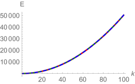
(a) Total Energy

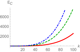
(b) Cross Helicity

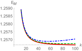
(c) Magnetic Helicity

Figure 2: Plots of absolute equilibrium states for absolute values of spectral quantities for Hall MHD. The parameters chosen are $\alpha=10$, $\beta=5$, $d_{i}=0.1$. The third parameter is varied with the solid red line corresponding to $\gamma=0.01$ with $\langle H_{C}\rangle/\langle H\rangle\approx 0.03$, the dashed green line corresponding to $\gamma=0.03$ with $\langle H_{C}\rangle/\langle H\rangle\approx 0.09$, and the dot-dashed blue line corresponding to $\gamma=0.05$ with $\langle H_{C}\rangle/\langle H\rangle\approx 0.16$. The spectral range is chosen to be $1<k<d_{i}^{-2}$.

Hence, we sum up this preliminary analysis by observing that $\mathcal{K}_{+}$ can undergo both forward and inverse cascades as predicted by Banerjee and Galtier (2016). We have also verified that our XMHD spectra, in the Hall MHD limit, are equal to the ones obtained earlier by Servidio et al. (2008).

IV.4 Inertial MHD Cascades

We begin by recalling that inertial MHD is a model which lacks the Hall drift, but is endowed with electron inertia effects (Kimura and Morrison, 2014; Lingam et al., 2015b). Thus, the existence of the second condition implies that the model may become relevant in the range $k\gg d_{e}^{-1}$, i.e. at scales smaller than electron skin depth. Although this quantity is small in many fusion plasmas, recall that it is highly relevant in astrophysical and space plasmas, such as the Earth’s magnetosphere and the solar wind. With this choice of $k$, observe that $d\approx\alpha/k^{2}d_{e}^{2}$ holds true.

Following the same procedure as in Hall MHD, we analyze the necessary inequalities, and find that

$$\alpha>k|\beta|d_{e}^{2}\quad\text{and}\quad\alpha\gtrsim|\gamma|.$$ (64)

Although $d_{e}\ll 1$, we also have $kd_{e}\gg 1$ in this case, and hence the condition $\alpha\gtrsim|\beta|$ appears to be quite reasonable. We also must inspect a counterpart of the third inequality in (42), which according to the constraints listed above collapses to

$$|\gamma|<\frac{\alpha}{kd_{e}}-|\beta|d_{e}.$$ (65)

Upon computation, the spectra become

$$E_{K} = E_{B}=\frac{8\pi\alpha}{d_{e}^{2}}\frac{\dfrac{\alpha^{2}}{k^{2}d_{e}^{2}}-\beta^{2}d_{e}^{2}-\gamma^{2}}{\Big{(}\beta^{2}+\dfrac{\alpha^{2}}{k^{2}d_{e}^{2}}-\gamma^{2}\Big{)}^{2}-\dfrac{4\alpha^{2}}{\beta^{2}k^{2}}},$$ (66)

$$E_{M} = -16\pi\beta k^{2}d_{e}^{2}\frac{\dfrac{\alpha^{2}}{k^{2}d_{e}^{2}}+\gamma^{2}-\beta^{2}d_{e}^{2}}{\Big{(}\beta^{2}+\dfrac{\alpha^{2}}{k^{2}d_{e}^{2}}-\gamma^{2}\Big{)}^{2}-\dfrac{4\alpha^{2}}{\beta^{2}k^{2}}},$$ (67)

$$E_{C} = -16\pi\gamma k^{2}\frac{\beta^{2}d_{e}^{2}+\dfrac{\alpha^{2}}{k^{2}d_{e}^{2}}-\gamma^{2}}{\Big{(}\beta^{2}+\dfrac{\alpha^{2}}{k^{2}d_{e}^{2}}-\gamma^{2}\Big{)}^{2}-\dfrac{4\alpha^{2}}{\beta^{2}k^{2}}}.$$ (68)

An important and pleasing feature is immediately apparent. We see that inertial MHD restores the energy equipartition feature of ideal MHD (Shivamoggi, 2015). This is along expected lines, since inertial MHD and ideal MHD are very akin to each other. In fact, it was shown by Lingam et al. (2015b) in 2D that the Hamiltonian (Poisson bracket) structure of these two models is identical under the transformation ${\bf B}\rightarrow{\bf B}^{*}$.

We also see that the generalized magnetic and cross helicities vanish when $\beta$ and $\gamma$ are set to zero respectively. Hence, it is instructive to take these two limits and inspect the resultant expressions. When $\beta=0$, the total energy is

$$E=\dfrac{16\pi\alpha}{\dfrac{\alpha^{2}}{k^{2}}-\gamma^{2}d_{e}^{2}},$$ (69)

and the cross-helicity is

$$E_{C}=-E\frac{\gamma}{\alpha}k^{2}d_{e}^{2}.$$ (70)

The other case, with $\gamma=0$, corresponds to the state with zero cross-helicity. In this instance, we find that the spectra are

$$E=\dfrac{16\pi\alpha}{\dfrac{\alpha^{2}}{k^{2}}-\beta^{2}d_{e}^{4}}\quad\text{and}\quad E_{M}=-E\frac{\beta}{\alpha}k^{2}d_{e}^{4}.$$ (71)

In each of these two limiting cases, we find that all spectral quantities undergo direct cascades in contrast to the MHD and Hall MHD limits. This appears to be consistent, to an extent, with previous results in the literature although most previous studies relied on 2D simulations as opposed to our 3D analysis (Biskamp et al., 1996, 1999; Dastgeer et al., 2000). We have plotted the spectra in Fig. 3, which confirms our theoretical predictions. Although the wavenumber range from $k$ to $1/d_{e}^{2}$, for inertial MHD is not applicable everywhere - instead, its presence is likely to be felt only when $k>1/d_{e}$. In reality, there is a finite Hall MHD range before this limit is attained.

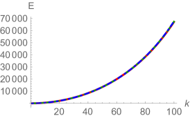
(a) Total Energy

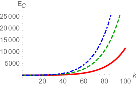
(b) Cross Helicity

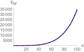
(c) Magnetic Helicity

Figure 3: Plots for absolute equilibria states of spectral quantities for inertial MHD. The parameters chosen are $\alpha=10$, $\beta=5$, $d_{e}=0.1$. The third parameter is varied with the solid red line corresponding to $\gamma=0.01$ with $\langle H_{C}\rangle/\langle H\rangle\approx 0.09$, the dashed green line to $\gamma=0.03$ with $\langle H_{C}\rangle/\langle H\rangle\approx 0.28$ and the dot-dashed blue line to $\gamma=0.05$ with $\langle H_{C}\rangle/\langle H\rangle\approx 0.46$. The spectral range is chosen to be $1<k<d_{e}^{-2}$.

We note, in passing, that the inclusion of a strong guide field can induce anisotropic turbulence, and the existence of both inverse and direct cascades, but this falls outside the scope of our present work.

V Discussion and Conclusion

There has been a great deal of attention in recent times focused on turbulence at ‘small’ scales, i.e., scales smaller than the electron or proton gyroradius (or skin depth). The two most notable examples in astrophysics are the Earth’s magnetosphere and the solar wind, respectively. The recently launched Magnetospheric Multiscale (MMS) Mission is known to be capable of probing such scales (Burch et al., 2016), and observational results in these regimes have also been recently published (Narita et al., 2016). We also note that probing such scales may also become feasible in the laboratory, such as the WiPAL (Forest et al., 2015).

Thus, in the coming years, it is likely that a thorough understanding of the physics at these scales will be necessary. To gain such an understanding, it is imperative to work with models that are applicable at such small scales. Neither ideal nor Hall MHD are valid when one approaches length scales on the order of the electron skin depth. As extended MHD (XMHD) is endowed with both the Hall drift and electron inertia, it constitutes a good physical model in this regime. Of course, we must caution the reader that it does not capture certain kinetic effects such as Landau damping, pressure anisotropy, etc. and also lacks dissipative effects.

In this paper, we have first focused on gaining a basic understanding of the salient mathematical properties of XMHD. This was done by taking recourse to the Hamiltonian formulation, which is endowed with several advantages. In particular, we discussed how the mutually exclusive effects of electron inertia and the Hall current can be unified into a single framework. We also presented the helicities of XMHD that are generalizations of the magnetic/fluid helicity. This was done by demonstrating that they are topological invariants of XMHD and can be determined through the Hamiltonian approach.

All of these facts were duly invoked in the subsequent sections, where we focused on some aspects on XMHD turbulence. Firstly, we generalized the results of Banerjee and Galtier (2016), where the dissipation rates of Hall MHD were computed by using second order structure functions. We showed that our results, with electron inertia, still resembled the Hall MHD case, and reduced to the latter when the electron skin depth was vanishingly small. We also showed that, in the limit of infinite Reynolds number, the dissipation rates vanished when the Beltrami conditions were satisfied, thereby confirming earlier predictions.

Table 1: Direction of cascades in MHD, HMHD and IMHD. *When $\langle H_{C}\rangle\ll\langle H\rangle$

	Ideal MHD	Hall MHD	Inertial MHD
$E$	direct	direct	direct
$E_{M}$	inverse	inverse*	direct
$E_{C}$	direct	direct	direct
${K}_{-}$	inverse	inverse*	direct
${K}_{+}$	inverse	both	direct

The central theme of the paper, however, revolved around the issue of the directionality of the cascades of the helicities and the energy. Unlike ideal MHD, where a direct cascade of the energy and the inverse cascade of the magnetic helicity can be unambiguously predicted, the situation is rendered far more complex due to the Hall drift and electron inertia. We commenced our analysis by proving Liouville’s theorem for the first time for XMHD, which was necessary for constructing the absolute equilibrium states of XMHD. The latter were used to study the cascades of XMHD in two limiting regimes: (i) where the Hall term is important and the electron inertia terms unimportant, and (ii) vice-versa.

In the Hall regime, the energy and the magnetic helicity still exhibit direct and inverse cascading, respectively. However, the ion canonical helicity $\int_{D}d^{3}x\,\left({\bf A}+d_{i}{\bf V}\right)\cdot\left({\bf B}+d_{i}\nabla\times{\bf V}\right)$, which is a conserved quantity in Hall MHD, can undergo a cascade in either direction. We also verified that the magnetic and kinetic energy spectra are characterized by a lack of equipartition, which constitutes a staple and unique feature of Hall MHD (that is absent in ideal MHD). Each of these results were shown to be consistent with, or identical to, previous studies; see, for e.g. Servidio et al. (2008).

When electron inertia effects were taken to be dominant over the Hall term (the inertial MHD regime) we found that equipartition was recovered. In addition, we also found that all of the quantities, viz.  the energy and the two helicities, undergo direct cascading in this regime. Hence, we expect that the (generalized) magnetic helicity undergoes inverse cascading up to a certain length scale (for a given choice of the free parameters), and then undergoes a reversal, consequently ending up as a direct cascade. A summary of these results can be found in Table 1.

In addition to the aforementioned systems such as the solar wind and Earth’s magnetosphere, our results may also have significant consequences in other areas. The presence of the inverse cascade of magnetic helicity is intimately linked to the generation of magnetic fields via the dynamo mechanism (Brandenburg, 2001; Brandenburg and Subramanian, 2005; Alexakis et al., 2006). The existence of an inverse cascade has already been investigated in the Hall regime by Mininni et al. (2003, 2007); Lingam and Bhattacharjee (2016b). But, if this feature were to be non-operational at smaller scales, it may lead to non-trivial, potentially far reaching, consequences in dynamo theory. Lastly, our analysis is also likely to be of some relevance in turbulent reconnection, which remains an active and unresolved area of research (Servidio et al., 2011; Lazarian et al., 2012). Hence, on account of the aforementioned reasons, we suggest further analyses of this kind are timely and warranted.

In closing, we describe a couple of important avenues that can be explored by means of our formalism. To begin with, the 2D version (reduced XMHD) can also be subjected to the same treatment since its Hamiltonian structure and invariants have been thoroughly studied and classified (Grasso et al., 2016). Alternatively, electron-positron plasmas, which are produced both via high-intensity lasers in the laboratory (Mourou et al., 2006), and also occur in many astrophysical settings (Harding and Lai, 2006), have attracted a great deal of interest recently. The dynamical equations for these plasmas are characterized by the absence of the Hall term, and can be derived by adopting a procedure akin to Dungey (1958) and Lüst (1959). It is, therefore, advantageous to utilize the Hamiltonian structure for this model (Kawazura et al., 2016), to derive the corresponding invariants (such as the generalized helicities), and to carry out an analysis of the cascades and spectra along the lines of our present work.

In recent times, there has been a great deal of interest on the study of relativistic turbulence, given its importance in laboratory and astrophysical plasmas. Most of the works thus far have focused on computational or phenomenological studies, as seen from the likes of Kumar and Narayan (2009); Zhang and Yan (2011); Inoue et al. (2011); Zrake (2014). In contrast, it has recently been shown that relativistic MHD possesses a noncanonical Hamiltonian formulation (D’Avignon et al., 2015). Thus, it is evident that a study akin to the one presented herein could be undertaken for relativistic MHD as well. We conclude by observing that one can combine relativity and two-fluid effects to arrive at relativistic extended MHD, which is also known to have a Hamiltonian structure (Kawazura et al., 2016). On account of the model’s generality, we suggest that this could be used for constructing the spectra and cascades, and most of the results (and models) discussed here would automatically follow as limiting cases.