Windowed Green Function Method for
Nonuniform Open-Waveguide Problems

Abstract

This contribution presents a novel Windowed Green Function (WGF) method for the solution of problems of wave propagation, scattering and radiation for structures which include open (dielectric) waveguides, waveguide junctions, as well as launching and/or termination sites and other nonuniformities. Based on use of a “slow-rise” smooth-windowing technique in conjunction with free-space Green functions and associated integral representations, the proposed approach produces numerical solutions with errors that decrease faster than any negative power of the window size. The proposed methodology bypasses some of the most significant challenges associated with waveguide simulation. In particular the WGF approach handles spatially-infinite dielectric waveguide structures without recourse to absorbing boundary conditions, it facilitates proper treatment of complex geometries, and it seamlessly incorporates the open-waveguide character and associated radiation conditions inherent in the problem under consideration. The overall WGF approach is demonstrated in this paper by means of a variety of numerical results for two-dimensional open-waveguide termination, launching and junction problems.

1 Introduction

This paper considers the problem of evaluation of wave propagation and scattering in nonuniform open-waveguide structures. This is a problem of fundamental importance in a wide range of areas, including modeling and design of dielectric antenna systems, photonic and optical devices, dielectric RF transmission lines, etc. The numerical simulation of such structures presents significant challenges—in view of the unbounded character of the associated dielectric boundaries and propagation domains as well as the presence of radiating fields, inhomogeneities, and scattering obstacles.

The present contribution introduces an effective methodology for the solution of such nonuniform open-waveguide problems. Based on use of Green functions and integral equations akin to those used in the Method of Moments [18], and incorporating as a main novel element a certain “slow-rise” windowing function, the proposed Windowed Green Function approach (WGF) can be used to model, with high-order accuracy, highly-complex waveguide structures—without recourse to use of mode matching (which can be quite challenging in the open-waveguide context), absorbing boundary conditions, staircasing or time-domain simulations.

The finite-difference time-domain method (FDTD) is one of the simplest and most reliable extant methods for solution of open-waveguide problems. In the FDTD approach, unbounded domains are truncated by relying on absorbing boundary conditions or absorbing layers such as the PML [1]. Further, subpixel smoothing techniques [12] are often used in FDTD implementations to model material interfaces while maintaining second order accuracy—in spite of the staircasing that accompanies Cartesian discretization of curved boundaries. In order to obtain the frequency response from a FDTD simulation, finally, Fourier transforms in time are typically used. In spite of its usefulness, the FDTD approach does present a number of difficulties in the context of waveguide problems [19, p. 223] concerning (i) Illumination by specified waveguide modes and inadvertent excitation of unwanted modes; (ii) Necessary use of sufficiently large computational domains to allow decay of reactive fields; (iii) Need for substantially prolonged simulation times in order for spectral energy above the waveguide cutoff frequency to reach a given interaction structure of interest; and (iv) Necessary use of fine spatial and temporal discretizations to mitigate the numerical dispersion associated with the second-order accuracy of the method.

A few Green function methods for open-waveguide problems have also been proposed. The recent boundary-element method [20], for example, in which a conductive absorber is used to truncate the unbounded waveguide structure, requires the excitation source to lie within the computational domain. The source then produces a radiation field that decays as $\mathcal{O}(1/r)$ and thus limits the accuracy of the implementation. Other approaches for open-waveguide problems include perturbation methods [7, 6] which can effectively handle limited types of (sufficiently small) localized inhomogeneities.

Relying on the free space Green function and associated integral equations along the dielectric boundaries, the WGF method presented in this paper utilizes a slow-rise window function to truncate the infinite integrals while providing super-algebraically small error (that is, errors smaller than any negative power of the window size). The method can easily incorporate bound modes and arbitrary beams as illuminating sources, and it can treat general inhomogeneities and multiple arbitrarily oriented waveguides without difficulty.

The proposed use of slow-rise window functions has been previously found highly effective in the contexts of scattering by periodic rough surfaces [15, 2, 4] and obstacles in presence of layered-media [3, 17] as well as long-range volumetric propagation [5]. The implementation details vary from problem to problem; in the present open-waveguide context, for example, the treatment of incident fields and windowed integral operators differs significantly from those used previously.

This paper is organized as follows: Notations and mathematical background on the open-waveguide problem are presented in Sec. 2. The WGF method is then introduced in Sec. 3, which includes, in particular, an integration example which demonstrates in a very simple context the properties of the slow-rise windowing function. A variety of applications of the open-waveguide WGF method are presented in Sec. 4, demonstrating applicability to waveguide junctions (including couplers and sharp bends), dielectric antennas, focused beam illumination, and, for reference, an unperturbed waveguide for which the exact solution is known. In all cases the WGF method provides high accuracies in computing times of the order of seconds. Significant additional acceleration could be incorporated on the basis of equivalent sources and Fast Fourier Transforms, along the lines of reference [4]; such acceleration methods are not considered here in view of the fast performance that the unaccelerated method already provides in the present two-dimensional case. Sec. 5, finally, highlights the properties of the method, and presents a few concluding remarks.

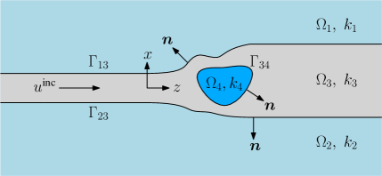
(a) Schematic depiction of a typical waveguide scattering problem.

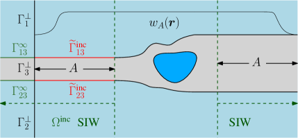
(b) Notations associated with this paper’s WGF method.

Figure 1: The open-waveguide problem and geometrical structures utilized in the WGF method presented in this paper.

2 Mathematical Framework for 2D Open Waveguides

This paper considers the problem of electromagnetic wave propagation and scattering induced by two-dimensional ($zx$-plane) nonuniform open (dielectric) waveguides, with application to nonuniformities such as waveguide junctions, illumination and termination regions. In Fig. 1 a schematic depiction of the problem is presented.

General two-dimensional structures consisting of spatial arrangements of two-dimensional dielectric waveguides and bounded dielectric structures can be considered within the proposed framework—including, for example, configurations which are constructed as a combination of a given finite number of “semi-infinite waveguide” structures (SIW) and additional bounded dielectric bodies. Here a SIW is one of the two portions that result as a fully uniform waveguide is cut by a straight line (plane) orthogonal to the waveguide axis. A simple such configuration is depicted in Fig. 1.

Additionally, it is useful to identify connected (bounded or unbounded) regions that are occupied by a given dielectric material; as illustrated in Fig. 1, in this paper these regions are denoted by $\Omega_{j}$ ($j=1,\dots,N$). The electrical permittivity, magnetic permeability, refractive indices and wavenumbers in $\Omega_{j}$ are denoted $\varepsilon_{j}$, $\mu_{j}$, $n_{j}$ and $k_{j}=\omega\sqrt{\varepsilon_{j}\mu_{j}}=n_{j}\omega/c$ ($c$ being the speed of light in vacuum), respectively.

The structure may be illuminated by arbitrary combinations of bound waveguide modes supported on a single component SIW (or, more precisely, by the restriction to the given SIW of a mode of the corresponding fully uniform waveguide). By linearity, simultaneous illumination by several SIWs can be obtained directly by addition of the corresponding solutions for single SIW illumination. Letting $\boldsymbol{r}=(z,x)$ and denoting by $\mathbf{\chi}^{\text{inc}}$ the indicator function of a SIW region $\Omega^{\text{inc}}$ that contains the prescribed illuminating field,

$$\mathbf{\chi}^{\text{inc}}(\boldsymbol{r})=\begin{cases}1&\text{for }\boldsymbol{r}\in\Omega^{\text{inc}}\\ 0&\text{for }\boldsymbol{r}\not\in\Omega^{\text{inc}},\end{cases}$$ (1)

the total electric field $\boldsymbol{E}$ is given by $\boldsymbol{E}=\boldsymbol{E}^{\text{inc}}\mathbf{\chi}^{\text{inc}}+\boldsymbol{E}^{\text{scat}}$. (See Fig. 1b, where the region $\Omega^{\text{inc}}=\{z<0\}$ is such that the waveguide boundaries are flat within $\Omega^{\text{inc}}$, and thus, a bound mode can be prescribed in this region as an incident field.) The scattered field $\boldsymbol{E}^{\text{scat}}$ is assumed to satisfy an appropriate radiation condition (which, roughly, states that the scattered field propagates away from all inhomogeneities as either outward waveguide modes or cylindrical waves; see [16, Eq. (24)] for details) in each component $\Omega_{j}$ that is not bounded —in addition to the Maxwell equations which, in the two-dimensional case considered in what follows, reduce to the Helmholtz equation.

Assuming a time-harmonic temporal dependence of the form $\operatorname{e}^{-i\omega t}$ (which is suppressed in all expressions in this paper) and letting $u$ (resp. $u^{\text{scat}}$) denote either the $y$-component of the total (resp. scattered) electric field in TE-polarization or the $y$-component of the total (resp. scattered) magnetic field in TM-polarization, the field component $u=u^{\text{inc}}\chi^{\text{inc}}+u^{\text{scat}}$ is the unique [16] radiating solution of the problem

$$\left\{\begin{array}[]{rcccc}\Delta u+k_{j}^{2}u&=&0&\text{in}&\Omega_{j},\vskip 3.0pt plus 1.0pt minus 1.0pt\\ u_{+}-u_{-}&=&0&\text{on}&\Gamma_{j\ell}\;\;(j<\ell),\vskip 6.0pt plus 2.0pt minus 2.0pt\\ \displaystyle\frac{\partial u_{+}}{\partial\boldsymbol{n}}-{\nu_{j\ell}}\frac{\partial\displaystyle u_{-}}{\partial\boldsymbol{n}}&=&0&\text{on}&\Gamma_{j\ell}\;\;(j<\ell).\end{array}\right.$$ (2)

Here $\nu_{j\ell}=1$ in TE-polarization and $\nu_{j\ell}=(k_{j}/k_{\ell})^{2}$ in TM-polarization; for each pair $(j,\ell)$ with $j<\ell$, $\Gamma_{j\ell}$ denotes the boundary between $\Omega_{j}$ and $\Omega_{\ell}$; for $\boldsymbol{r}\in\Gamma_{j\ell}$, $\boldsymbol{n}=\boldsymbol{n}(\boldsymbol{r})$ denotes the unit normal vector to $\Gamma_{j\ell}$ which points into the “plus side” $\Omega_{j}$ of $\Gamma_{j\ell}$ (the plus side of $\Gamma_{j\ell}$ is defined by the aforementioned condition $j<\ell$); and for $\boldsymbol{r}\in\Gamma_{j\ell}$, finally,

$$u_{\pm}(\boldsymbol{r})=\lim_{\delta\to 0^{+}}\big{[}u(\boldsymbol{r}\pm\delta\boldsymbol{n}(\boldsymbol{r}))\big{]}\quad\mbox{and}\quad\frac{\partial u_{\pm}}{\partial\boldsymbol{n}}(\boldsymbol{r})=\lim_{\delta\to 0^{+}}\big{[}\nabla u(\boldsymbol{r}\pm\delta\boldsymbol{n}(\boldsymbol{r}))\cdot\boldsymbol{n}(\boldsymbol{r})\big{]}.$$ (3)

Remark 2.1.

A few comments concerning notations are in order: (i) $\Gamma_{j\ell}$ may be empty for a number of pairs $(j,\ell)$: for example $\Gamma_{12}=\emptyset$ for the geometry displayed in Fig. 1a, and $\Gamma_{j\ell}$ is necessarily empty, by definition, whenever $j\geq\ell$. (ii) The use of indicator functions (1) makes it possible to conveniently specify incident fields in an adequately selected SIW region $\Omega^{\text{inc}}$ (which equals the half plane containing the SIW that supports the incident field). (iii) Once $u$ is determined by solving (2), the total electromagnetic field in the domain $\Omega_{j}$ ($j=1,2\dots N$) is given by $\boldsymbol{E}=(0,u,0)$, $\boldsymbol{H}=\frac{i}{\omega\mu_{j}}\left(\frac{\partial u}{\partial z},0,-\frac{\partial u}{\partial x}\right)$ in TE-polarization, and $\boldsymbol{E}=\frac{i\omega\mu_{j}}{k_{j}^{2}}\left(-\frac{\partial u}{\partial z},0,\frac{\partial u}{\partial x}\right)$, $\boldsymbol{H}=\left(0,u,0\right)$ in TM-polarization.

3 Windowed Green Function Method (WGF)

3.1 Integral Equation Formulation

This section presents an integral equation formulation for the propagation and scattering problem considered in Sec. 2. For simplicity, it is assumed that the structure is illuminated by means of an arbitrary superposition of bound modes incoming from a single SIW whose optical axis coincides with the $z-$axis; the generalization to structures containing multiple arbitrarily-oriented waveguides is straightforward. Under this assumption, the incident field is prescribed by

$$u^{\text{inc}}(z,x)=\sum_{m=1}^{M}A^{\text{inc}}_{m}u^{m}_{\perp}(x)\operatorname{e}^{ik^{m}_{z}z},$$ (4)

where $M$ is the total number of bound modes supported by the waveguide structure, $A^{\text{inc}}_{m}$ denotes the $m$-th modal coefficient, $u^{m}_{\perp}(x)$ is the transverse profile of the mode, and $k^{m}_{z}$ is the corresponding propagation constant for the $m$-th mode. Note that $u^{m}_{\perp}(x)$ and $k^{m}_{z}$ can be easily found by solving a one dimensional eigenvalue problem by means of the method of separation of variables [14]. For example, the bound mode solutions for a single waveguide centered at $x=0$, with half-width $h$ and with core and cladding wavenumbers $k_{\text{co}}>k_{\text{cl}}$ respectively, are given by [14]

$$u_{\perp}^{m}(x)=\begin{cases}v\left(\gamma_{\text{co}}~{}h\right)e^{-\gamma_{\text{cl}}(x-h)}&,\quad x>h\\ v\left(\gamma_{\text{co}}~{}x\right)&,\quad|x|\leq h\\ v\left(-\gamma_{\text{co}}~{}h\right)e^{\gamma_{\text{cl}}(x+h)}&,\quad x<-h,\\ \end{cases}$$ (5)

where $\gamma_{\text{co}}=\sqrt{k_{\text{co}}^{2}-{(k_{z}^{m})}^{2}}$ and $\gamma_{\text{cl}}=\sqrt{{(k_{z}^{m})}^{2}-k_{\text{cl}}^{2}}$. Here $v(\tau)=\cos(\tau)$ for the symmetric modes, $v(\tau)=\sin(\tau)$ for the antisymmetric modes, and $k^{m}_{z}$ ($k_{\text{cl}}<k^{m}_{z}<k_{\text{co}}$) is the $m$-th solution of the transcendental equation

$$\begin{cases}\displaystyle\gamma_{\text{cl}}=\nu_{\text{wg}}\gamma_{\text{co}}\tan{\left(\gamma_{\text{co}}h\right)}&\text{(symmetric mode),}\\ \displaystyle\nu_{\text{wg}}\gamma_{\text{co}}=-\gamma_{\text{cl}}\tan{\left(\gamma_{\text{co}}h\right)}&\text{(antisymmetric mode),}\end{cases}$$ (6)

with $\nu_{\text{wg}}=1$ for TE-polarization and $\nu_{\text{wg}}=(k_{\text{cl}}/k_{\text{co}})^{2}$ for TM-polarization. As indicated in Sec. 4, further, additional incident fields such as plane waves, and finite beams can also be incorporated easily in this context.

In order to introduce the desired system of integral equations, let $\Gamma_{j}=\left(\bigcup_{\ell=1}^{j-1}\Gamma_{\ell j}\right)\bigcup\left(\bigcup_{\ell=j+1}^{N}\Gamma_{j\ell}\right)$ denote the boundary of the domain $\Omega_{j}$ and let $\Gamma=\bigcup_{j=1}^{N}\Gamma_{j}$ denote the union of all domain boundaries. Then, calling

$$\varphi(\boldsymbol{r})\equiv u_{+}(\boldsymbol{r})\quad\text{and}\quad\psi(\boldsymbol{r})\equiv\frac{\partial u_{+}}{\partial\boldsymbol{n}}(\boldsymbol{r}),\quad\boldsymbol{r}\in\Gamma,$$ (7)

and using Green’s theorem in a manner akin to [11] together with the boundary conditions in (2), the representation formula

$$u(\boldsymbol{r})=\mathscr{D}[\beta_{j}\varphi](\boldsymbol{r})-\mathscr{S}\left[\beta_{j}\nu_{j}^{-1}\psi\right](\boldsymbol{r}),\quad\boldsymbol{r}\in\Omega_{j}$$ (8)

results, where

$$\beta_{j}(\boldsymbol{r})=\begin{cases}\;\;\;1,&\text{for }\boldsymbol{r}\in\Gamma_{j\ell}\;(j<\ell)\\ -1,&\text{for }\boldsymbol{r}\in\Gamma_{\ell j}\;(j>\ell)\end{cases},\quad \quad\nu_{j}(\boldsymbol{r})=\begin{cases}1,&\text{for }\boldsymbol{r}\in\Gamma_{j\ell}\;(j<\ell)\\ \nu_{\ell j},&\text{for }\boldsymbol{r}\in\Gamma_{\ell j}\;(j>\ell)\end{cases},$$ (9)

$$\nu(\boldsymbol{r})=\nu_{\ell j},\quad\text{for }\boldsymbol{r}\in\Gamma_{j\ell}\;(j<\ell),$$ (10)

and where, letting $G_{j}(\boldsymbol{r},\boldsymbol{r}^{\prime})=\frac{i}{4}H_{0}^{(1)}(k_{j}|\boldsymbol{r}-\boldsymbol{r}^{\prime}|)$ denote the free-space Green function for the Helmholtz equation with wavenumber $k_{j}$, the single and double layer potentials $\mathscr{S}$ and $\mathscr{D}$ for a given density $\eta$ defined in $\Gamma$ are given by

$$\mathscr{S}[\eta](\boldsymbol{r})=\int_{\Gamma_{j}}G_{j}(\boldsymbol{r},\boldsymbol{r}^{\prime})\eta(\boldsymbol{r}^{\prime}){d}s_{\boldsymbol{r}^{\prime}}\quad\text{and}\quad\displaystyle\mathscr{D}[\eta](\boldsymbol{r})=\int_{\Gamma_{j}}\frac{\partial G_{j}}{\partial\boldsymbol{n}(\boldsymbol{r}^{\prime})}(\boldsymbol{r},\boldsymbol{r}^{\prime})\eta(\boldsymbol{r}^{\prime}){d}s_{\boldsymbol{r}^{\prime}},\quad\text{for }\boldsymbol{r}\in\Omega_{j}.$$ (11)

The densities $\varphi$ and $\psi$ in the representation formula (8), which, in view of equation (7), are given in terms of the total field, can be expressed as a sum of their incident and scattered components. In other words $\varphi=\varphi^{\text{inc}}+\varphi^{s}$ and $\psi=\psi^{\text{inc}}+\psi^{\text{scat}}$ where, using the indicator function (1),

$$\varphi^{\text{inc}}(\boldsymbol{r})\equiv\chi^{\text{inc}}u^{\text{inc}}_{+}(\boldsymbol{r})~{}~{} \text{and}~{}~{}\psi^{\text{inc}}(\boldsymbol{r})\equiv\chi^{\text{inc}}\frac{\partial u^{\text{inc}}_{+}}{\partial\boldsymbol{n}}(\boldsymbol{r}),~{}~{}\boldsymbol{r}\in\Gamma,$$ (12)

$$\varphi^{\text{scat}}(\boldsymbol{r})\equiv u^{\text{scat}}_{+}(\boldsymbol{r})~{}~{} \text{and}~{}~{}\psi^{\text{scat}}(\boldsymbol{r})\equiv\frac{\partial u^{\text{scat}}_{+}}{\partial\boldsymbol{n}}(\boldsymbol{r}),~{}~{}\boldsymbol{r}\in\Gamma.$$ (13)

The desired integral equations for the unknown densities $\varphi^{\text{scat}}$ and $\psi^{\text{scat}}$ are expressed in terms of certain free-space Green functions and various associated integral operators. The particular Green function used in the definition of each one of these operators depends on $\boldsymbol{r}$: for $\boldsymbol{r}\in\Gamma_{j\ell}$ a “plus” (resp. “minus”) operator uses the Green function $G_{j}$ (resp. $G_{\ell}$) corresponding to the refractive index on the plus side (resp. minus side) of $\Gamma_{j\ell}$. To streamline the notations in this context, for $\boldsymbol{r}\in\Gamma$ let $\Gamma^{\pm}(\boldsymbol{r})$ be defined as follows: if $\boldsymbol{r}\in\Gamma_{j\ell}$ then $\Gamma^{+}(\boldsymbol{r})=\Gamma_{j}$ and $\Gamma^{-}(\boldsymbol{r})=\Gamma_{\ell}$ (cf. Remark 2.1). The aforementioned integral operators are thus defined by

$$\begin{array}[]{r c l r c l}\displaystyle S^{\pm}[\eta](\boldsymbol{r})&=&\displaystyle\int_{\Gamma^{\pm}(\boldsymbol{r})}G^{\pm}(\boldsymbol{r},\boldsymbol{r}^{\prime})\eta(\boldsymbol{r}^{\prime})ds_{\boldsymbol{r}^{\prime}},&\displaystyle D^{\pm}[\eta](\boldsymbol{r})&=&\displaystyle\int_{\Gamma^{\pm}(\boldsymbol{r})}\frac{\partial G^{\pm}(\boldsymbol{r},\boldsymbol{r}^{\prime})}{\partial\boldsymbol{n}(\boldsymbol{r}^{\prime})}\eta(\boldsymbol{r}^{\prime})ds_{\boldsymbol{r}^{\prime}},\\[14.22636pt] \displaystyle K^{\pm}[\eta](\boldsymbol{r})&=&\displaystyle\int_{\Gamma^{\pm}(\boldsymbol{r})}\frac{\partial G^{\pm}(\boldsymbol{r},\boldsymbol{r}^{\prime})}{\partial\boldsymbol{n}(\boldsymbol{r})}\eta(\boldsymbol{r}^{\prime})ds_{\boldsymbol{r}^{\prime}},&\displaystyle N^{\pm}[\eta](\boldsymbol{r})&=&\displaystyle\int_{\Gamma^{\pm}(\boldsymbol{r})}\frac{\partial^{2}G^{\pm}(\boldsymbol{r},\boldsymbol{r}^{\prime})}{\partial\boldsymbol{n}(\boldsymbol{r})\partial\boldsymbol{n}(\boldsymbol{r}^{\prime})}\eta(\boldsymbol{r}^{\prime})ds_{\boldsymbol{r}^{\prime}}\end{array}(\boldsymbol{r}\in\Gamma).$$ (14)

As is known (cf. [9] theorems 3.1 and 3.2), the layer potentials (11) satisfy the jump conditions at $\boldsymbol{r}\in\Gamma$:

$$\begin{array}[]{r c l r c l}\displaystyle\lim_{\delta\to 0^{+}}\mathscr{S}[\eta](\boldsymbol{r}\pm\delta\boldsymbol{n}(\boldsymbol{r}))&=&S^{\pm}[\eta](\boldsymbol{r}),&\displaystyle\lim_{\delta\to 0^{+}}\mathscr{D}[\eta](\boldsymbol{r}\pm\delta\boldsymbol{n}(\boldsymbol{r}))&=&\displaystyle\pm\frac{1}{2}\eta(\boldsymbol{r})+D^{\pm}[\eta](\boldsymbol{r}),\\[14.22636pt] \displaystyle\lim_{\delta\to 0^{+}}\frac{\partial}{\partial\boldsymbol{n}}\mathscr{D}[\eta](\boldsymbol{r}\pm\delta\boldsymbol{n}(\boldsymbol{r}))&=&N^{\pm}[\eta](\boldsymbol{r}),&\displaystyle\lim_{\delta\to 0^{+}}\frac{\partial}{\partial\boldsymbol{n}}\mathscr{S}[\eta](\boldsymbol{r}\pm\delta\boldsymbol{n}(\boldsymbol{r}))&=&\displaystyle\mp\frac{1}{2}\eta(\boldsymbol{r})+K^{\pm}[\eta](\boldsymbol{r}).\end{array}$$ (15)

Thus, adding the limits of the fields (8) (resp. the normal derivatives of the fields (8)) on the plus and minus sides of $\Gamma$, the system of integral equations

$$E(\boldsymbol{r})\boldsymbol{\phi}^{\text{scat}}(\boldsymbol{r})+T[\boldsymbol{\phi}^{\text{scat}}](\boldsymbol{r})=-E(\boldsymbol{r})\boldsymbol{\phi}^{\text{inc}}(\boldsymbol{r})-T[\boldsymbol{\phi}^{\text{inc}}](\boldsymbol{r}),\quad\text{for }\boldsymbol{r}\in\Gamma,$$ (16)

results, where

$$E(\boldsymbol{r})=\text{diag}\left[1,\frac{1+\nu(\boldsymbol{r})}{2\nu(\boldsymbol{r})}\right],\quad T=\begin{bmatrix}\displaystyle D^{-}-D^{+}&\displaystyle S^{+}-(1/\nu)S^{-}\\ \displaystyle N^{-}-N^{+}&\displaystyle K^{+}-(1/\nu)K^{-}\end{bmatrix},$$ (17)

and where the density vectors are given by

$$\boldsymbol{\phi}^{\text{scat}}=[\varphi^{\text{scat}},\psi^{\text{scat}}]^{t},\quad\text{and}\quad\boldsymbol{\phi}^{\text{inc}}=[\varphi^{\text{inc}},\psi^{\text{inc}}]^{t}.$$ (18)

3.2 Oscillatory integrals and the slow-rise windowing function

Special considerations must be taken into account in order to solve the system of equations (16) numerically—mainly in view of the slow decay of the associated integrands (equation (14)) for a fixed target point $\boldsymbol{r}\in\Gamma$ as $\boldsymbol{r}^{\prime}\to\infty$. A direct truncation of the integration domain (i.e., replacement of the integrals in (14) by corresponding integrals over the domain $\Gamma^{\pm}(\boldsymbol{r})\cap\{|\boldsymbol{r}|\leq A\}$) yields slow convergence, on account of edge effects, as the size $A$ of the truncation domain tends to infinity. Relying on a certain slow-rise windowing technique that smoothly truncates the integration domain, the proposed approach addresses this difficulty—and, in fact, it gives rise to a super-algebraically convergent algorithm. The resulting windowed integral equations can be subsequently discretized by means of any integral solver, including, in particular, the Method of Moments [18], or, indeed, any Nyström, Galerkin or collocation approach. The particular implementations presented in this paper are based on the high-order Nyström method described in [9, Sec. 3.5].

The proposed methodology is based on use of an infinitely smooth function $w_{A}(z)$, defined for $z\in\mathbb{R}$, which satisfies the following properties: (i) $w_{A}(z)$ vanishes for $z$ outside the interval $[-A,A]$; (ii) $w_{A}(z)$ equals 1 for $z\in(-\alpha A,\alpha A)$ for some $\alpha$ satisfying $0<\alpha<1$; (iii) All of the derivatives $w_{A}^{(p)}(z)$ ($p$ a positive integer) vanish at $z=\pm A$ and $z=\pm\alpha A$; and (iv) $w_{A}(z)$ exhibits a “slow-rise” from $0$ to $1$ as $|z|$ goes from $|z|=\pm\alpha A$ to $|z|=A$—in the sense that each derivative of $w_{A}$, of any given order, tends to zero everywhere (and, in particular, in the rise intervals $\alpha A\leq|z|\leq A$) as $A\to\infty$. The windowing function used in this paper is given by

$$w_{A}(z)=\begin{cases}1,&s<0\\ \displaystyle\exp{\bigg{(}-2\frac{\exp{(-1/|s|^{2})}}{|1-s|^{2}}\bigg{)}},&\displaystyle 0\leq s\leq 1,\hskip 22.76228pts(z)=\frac{|z|-\alpha A}{A(1-\alpha)}\\ 0,&s>0\end{cases},$$ (19)

but other choices could be equally suitable [2]. As shown in that reference and demonstrated by means of a simple example in Sec. 3.3, such windowing functions can be used to evaluate, with super-algebraic accuracy, certain improper integrals with slowly decaying oscillatory integrands—like the integrands in equation (14); see Remark 3.1.

Remark 3.1.

In view of the asymptotic expressions for the Hankel function, each one of the integral kernels involved in the equation system (16) can be expressed in the form $h(t)\exp{(it)}$ where $t=k|\boldsymbol{r}-\boldsymbol{r}^{\prime}|=k|z-z^{\prime}|\sqrt{1+(\frac{x-x^{\prime}}{z-z^{\prime}})^{2}}$ and where $h(t)\sim t^{-1/2}$ ($t\to\infty$) is a function each one of whose derivatives is bounded for all $t>1$ [13, Sec. 5.11] (see also [10, 3]). On the other hand, the scattered densities $\varphi^{\text{scat}}$ approach oscillatory asymptotic functions as $\boldsymbol{r}^{\prime}=(z^{\prime},x^{\prime})$ tends to infinity along $\Gamma^{\pm}(\boldsymbol{r})$ [16]: $\varphi^{\text{scat}}\sim\sum_{m}A^{\text{scat}}_{m}u^{m}_{\perp}(x^{\prime})e^{-ik_{z}^{m}|z^{\prime}|}$ as $z^{\prime}\rightarrow-\infty$ and $\varphi^{\text{scat}}\sim\sum_{n}B^{\text{scat}}_{n}u^{n}_{\perp}(x^{\prime})e^{ik_{z}^{n}|z^{\prime}|}$ as $z^{\prime}\rightarrow\infty$, with similar expressions for the density $\psi^{\text{scat}}$. Combining the kernel and density asymptotics it follows, in particular, that the net integrands in the operators (14) equals a sum of slowly decaying oscillatory functions with wavenumbers $\pm(k+k_{z}^{n})$.

3.3 Error estimates for a simplified windowed integral

In order to illustrate the properties of the windowed-integration method used in this paper it is useful to consider here a simple integration problem presented in [2], namely, the problem of numerical evaluation of the integral

$$I=\int_{1}^{\infty}\frac{\operatorname{e}^{iaz}}{\sqrt{z}}dz;$$ (20)

see, in particular, [2, theorem 3.1]. Letting $I_{\text{tr}}(A)=\int_{1}^{A}\frac{\operatorname{e}^{iaz}}{\sqrt{z}}dz$, $I_{w}(A)=\int_{1}^{A}w_{A}(z)\frac{\operatorname{e}^{iaz}}{\sqrt{z}}dz,$ then, by definition $I=\lim_{A\rightarrow\infty}I_{\text{tr}}(A)$. As is known, the value of $I$ is finite—in spite of the slow decay of the integrand (the integral of the function $1/\sqrt{z}$ in the same domain is infinite!). The finiteness of the improper integral between $1$ and $\infty$, which results from cancellation of positive and negative contributions arising from the oscillatory factor $\operatorname{e}^{iaz}$, may be verified by integrating by parts the integral $I_{\text{tr}}(A)$ (differentiating $1/\sqrt{z}$ and integrating $\operatorname{e}^{iaz}$). This procedure produces two terms: (i) An integral with a more rapidly decaying integrand and whose convergence does not rely on cancellations, as well as (ii) Boundary contributions at $z=1$ and $z=A$. Besides establishing the existence of the the limit $\lim_{A\rightarrow\infty}I_{\text{tr}}(A)$, this expression tells us that the $z=A$ boundary contribution $1/(ia\sqrt{A})\operatorname{e}^{iaA}$ equals the error in the approximation of $I$ by $I_{\text{tr}}(A)$. On the other hand, use of integration by parts on $I_{w}(A)$ does not give rise to a boundary contribution for $z=A$—on account of the fact $w_{A}(A)=w_{A}^{\prime}(A)=0$. In fact, since all the derivatives of $w_{A}(z)$ vanish at $z=A$, the integration by parts procedure can be performed on $I_{w}(A)$ an arbitrary number $p$ of times without ever producing a boundary contribution—a fact which lies at the heart of the accuracy resulting from the slow-rise windowing approach. As shown in [2, theorem 3.1] this procedure leads to the error estimates

$$|I-I_{\text{tr}}(A)|=\mathcal{O}\left(\frac{1}{a\sqrt{A}}\right),$$ (21)

$$|I-I_{w}(A)|=\mathcal{O}\left(\frac{1}{\sqrt{a}(aA)^{p-\frac{1}{2}}}\right)\;\text{for every }p\geq 1,$$ (22)

which are corroborated by the results in Table 1.

A	$\displaystyle|I-I_{\text{tr}}(A)|$	$\displaystyle|I-I_{w}(A)|$
10	$5.0\times 10^{-2}$	$3.6\times 10^{-3}$
20	$3.6\times 10^{-2}$	$5.8\times 10^{-5}$
25	$3.2\times 10^{-2}$	$9.3\times 10^{-6}$
50	$2.2\times 10^{-2}$	$3.1\times 10^{-9}$
75	$1.8\times 10^{-2}$	$3.1\times 10^{-12}$
100	$1.6\times 10^{-2}$	$1.0\times 10^{-14}$

Table 1: Convergence of the windowed integrals $I_{\text{tr}}(A)$ and $I_{w}(A)$ with $a=2\pi$ and window parameter $\alpha=0.5$

3.4 Windowed integral equations

Per Remark 3.1, for a fixed $\boldsymbol{r}\in\Gamma$ the integrands associated with the operators on the left-hand side of equation (16) are oscillatory and slowly decaying at infinity—just like the integrand in the simplified example presented in Sec. 3.3. Thus, it is expected that use of windowing in the integrands of the aforementioned operators should result in convergence properties analogous to the ones described in that section. Since the integrands on the right-hand side (RHS) of equation (16) are known functions, and since, as shown below, the full RHS can be evaluated efficiently (by relying on equation (25)), the use of windowing may be restricted to the left-hand operators.

These considerations lead to the following system of “windowed” integral equations on the bounded domain $\widetilde{\Gamma}=\Gamma\cap\{w_{A}(\boldsymbol{r})\neq 0\}$:

$$E(\boldsymbol{r})\boldsymbol{\phi}_{w}^{\text{scat}}(\boldsymbol{r})+T[w_{A}\boldsymbol{\phi}_{w}^{\text{scat}}](\boldsymbol{r})=-E(\boldsymbol{r})\boldsymbol{\phi}^{\text{inc}}(\boldsymbol{r})-T[\boldsymbol{\phi}^{\text{inc}}](\boldsymbol{r}),\quad\text{for }\boldsymbol{r}\in\widetilde{\Gamma}.$$ (23)

A discrete version of equations (23) can be obtained by substituting all left-hand side integrals by adequate quadrature rules (as mentioned above, the Nyström method [9, Sec. 3.5] is used for this purpose in this paper). The windowing function $w_{A}(\boldsymbol{r})$ used here is selected as follows: (i) $w_{A}=1$ on any portion of $\Gamma$ that is not part of a SIW; (ii) $w_{A}$ varies smoothly, with values between 0 and 1, along any portion of $\Gamma$ contained in a SIW, in a manner akin to that inherent in the windowing function used in Sec. 3.3, and; (iii) on each SIW, the center of the $\{w_{A}(\boldsymbol{r})=1\}$ region lies at the edge of the SIW (see Fig. 1b). As demonstrated in Sec. 4 through a variety of numerical results, the solution $\boldsymbol{\phi}_{w}^{\text{scat}}$ of equation (23) provides a super-algebraically accurate approximation to $\boldsymbol{\phi}^{\text{scat}}$ throughout the region $\{w_{A}(\boldsymbol{r})=1\}$.

While in principle the integrals $T[\boldsymbol{\phi}^{\text{inc}}](\boldsymbol{r})$ on the RHS in equation (23) could be computed on the basis of windowing functions, an alternative numerical approach was found preferable. To introduce this alternative strategy consider the discussion leading to equation (16). Clearly, the first (resp. second) component in the quantity $(\xi,\eta)^{t}=T[\boldsymbol{\phi}^{\text{inc}}](\boldsymbol{r})$ for $\boldsymbol{r}\in\widetilde{\Gamma}$ is given by the limit as $\boldsymbol{r}$ tends to $\widetilde{\Gamma}$ of the field $u$ (resp. the normal derivative of the field $u$) that results as the pair $(\phi,\psi)^{t}$ in (8) is replaced by the incident densities $(\phi^{\text{inc}},\psi^{\text{inc}})^{t}(=\boldsymbol{\phi}^{\text{inc}})$. Note that, per equation (12), $\boldsymbol{\phi}^{\text{inc}}$ vanishes identically outside $\Gamma_{j}^{\text{inc}}=\Gamma_{j}\cap\Omega^{\text{inc}}$. Now, given that the illuminating structure is a single SIW whose optical axis coincides with the $z-$axis (as indicated in Sec. 3.1), the corresponding integration domain $\Gamma_{j}^{\text{inc}}$ can be decomposed as the union $\Gamma_{j}^{\text{inc}}=\widetilde{\Gamma}_{j}^{\text{inc}}\cup{\Gamma}_{j}^{\infty}$ of the two disjoint segments $\widetilde{\Gamma}_{j}^{\text{inc}}=\Gamma_{j}^{\text{inc}}\cap\{w_{A}(\boldsymbol{r})\neq 0\}$ and ${\Gamma}_{j}^{\infty}=\Gamma_{j}^{\text{inc}}\cap\{w_{A}(\boldsymbol{r})=0\}$. (With reference to Fig. 1b note that $\Gamma^{\text{inc}}_{j}=\left(\bigcup_{\ell=1}^{j-1}\Gamma_{\ell j}^{\text{inc}}\right)\bigcup\left(\bigcup_{\ell=j+1}^{N}\Gamma_{j\ell}^{\text{inc}}\right)$ where $\Gamma_{j\ell}^{\text{inc}}=\Gamma_{j\ell}\cap\Omega^{\text{inc}}$; similarly, $\widetilde{\Gamma}_{j}^{\text{inc}}$ and ${\Gamma}_{j}^{\infty}$ are decomposed as the unions of the curves $\widetilde{\Gamma}_{j\ell}^{\text{inc}}=\Gamma_{j\ell}^{\text{inc}}\cap\{w_{A}(\boldsymbol{r})\neq 0\}$ and $\Gamma_{j\ell}^{\infty}=\Gamma_{j\ell}^{\text{inc}}\cap\{w_{A}(\boldsymbol{r})=0\}$, respectively. Fig. 1b only displays the independent components $\widetilde{\Gamma}_{j\ell}^{\text{inc}}$ and $\Gamma_{j\ell}^{\infty}$.) Using the fact that the incident densities $\varphi^{\text{inc}}$ and $\psi^{\text{inc}}$ vanish outside $\Gamma_{j}^{\text{inc}}$, for $\boldsymbol{r}\in\Omega_{j}$ the relation

$$\displaystyle\mathscr{D}[\beta_{j}\varphi^{\text{inc}}](\boldsymbol{r})-\mathscr{S}\left[\beta_{j}\nu_{j}^{-1}\psi^{\text{inc}}\right](\boldsymbol{r})=\int_{\widetilde{\Gamma}_{j}^{\text{inc}}\cup{\Gamma}_{j}^{\infty}}\left[\frac{\partial G_{j}}{\partial\boldsymbol{n}(\boldsymbol{r}^{\prime})}(\boldsymbol{r},\boldsymbol{r}^{\prime})\varphi^{\text{inc}}(\boldsymbol{r}^{\prime})-G_{j}(\boldsymbol{r},\boldsymbol{r}^{\prime})\nu_{j}^{-1}\psi^{\text{inc}}(\boldsymbol{r}^{\prime})\right]\beta_{j}{d}s_{\boldsymbol{r}^{\prime}},$$ (24)

results. The evaluation of the right-hand integral is discussed in what follows.

The integral over the bounded curve $\widetilde{\Gamma}_{j}^{\text{inc}}$ in (24) can be computed using any of the standard singular-integration techniques mentioned in Sec. 3.2. The curve ${\Gamma}_{j}^{\infty}$ extends to infinity, on the other hand, with an integrand that decays slowly (see Remark 3.1). Fortunately, however, the ${\Gamma}_{j}^{\infty}$ integration problem can be significantly simplified by relying on the fact that $(\phi^{\text{inc}},\psi^{\text{inc}})^{t}(=\boldsymbol{\phi}^{\text{inc}})$ actually coincides with the boundary values of the incident field and its normal derivative, as indicated in equation (12). To evaluate the ${\Gamma}_{j}^{\infty}$ integral consider the identity

$$\int_{{\Gamma}_{j}^{\infty}} \left[\frac{\partial G_{j}}{\partial\boldsymbol{n}(\boldsymbol{r}^{\prime})}(\boldsymbol{r},\boldsymbol{r}^{\prime})\varphi^{\text{inc}}(\boldsymbol{r}^{\prime})-G_{j}(\boldsymbol{r},\boldsymbol{r}^{\prime})\nu_{j}^{-1}\psi^{\text{inc}}(\boldsymbol{r}^{\prime})\right]\beta_{j}{d}s_{\boldsymbol{r}^{\prime}}=$$

$$-\int_{\Gamma_{j}^{\perp}}\left[\frac{\partial G_{j}}{\partial\boldsymbol{n}(\boldsymbol{r}^{\prime})}(\boldsymbol{r},\boldsymbol{r}^{\prime})u_{+}^{\text{inc}}(\boldsymbol{r}^{\prime})-G_{j}(\boldsymbol{r},\boldsymbol{r}^{\prime})\nu_{j}^{-1}\frac{\partial u_{+}^{\text{inc}}}{\partial\boldsymbol{n}}(\boldsymbol{r}^{\prime})\right]\beta_{j}{d}s_{\boldsymbol{r}^{\prime}},\quad\text{for }\boldsymbol{r}\in\{z>-A\},$$ (25)

that results by using Green’s theorem in a manner akin to [11] (the corresponding bounded-domain result can be found e.g. in [8, theorem 3.1]). (Here $\Gamma_{j}^{\perp}=\Omega_{j}\cap\{z=-A\}$ is such that $\Gamma_{j}^{\perp}\cup{\Gamma}_{j}^{\infty}$ is the boundary of the region $\Omega_{j}\cap\{z<-A\}$, see Fig. 1b.) Equation (25) provides an alternative approach for the evaluation of the integrals over ${\Gamma}_{j}^{\infty}$ in equation (24). While some of the $\Gamma_{j}^{\perp}$ curves are unbounded, along such unbounded curves the fields decay exponentially fast (see equation (5)), and, thus, arbitrary accuracy can efficiently be achieved in the corresponding integrals by truncation of the integration domain to a relatively small bounded portion of $\Gamma_{j}^{\perp}$.

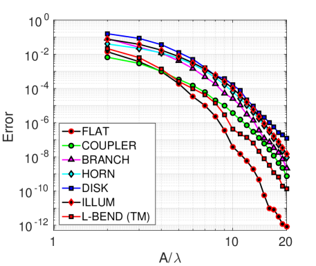
(a) Loglog plot

(b) Semilog plot

Figure 2: Super-algebraic convergence of the WGF method for various test configurations. In all cases a sufficiently fine numerical grid was used (eight to twelve points per wavelength) to ensure the leading error is caused by the WGF’s slow-rise boundary truncation. Here the scaled window size $A/\lambda$ is varied while $\lambda=\text{max}_{j}(2\pi/k_{j})$ is kept fixed (where the values of $k_{j}$ are described in the text for each test case).

The overall WGF method for open waveguides is summarized in points 1 to 3 below. As mentioned above in this paper, the bounded-interval numerical integrations mentioned in the points 1 to 3 can be effected by means of any numerical integration method applicable to the kinds of singular integrals (with singular kernels and, at corners, unknown singular densities) associated with the problems under consideration. The implementation used to produce the numerical results in Sec. 4 relies on numerical integration methods derived in a direct manner from those described in [9, Sec. 3.5].

The WGF algorithm proceeds as follows:

1. Evaluate the RHS of equation (23) by decomposing the integrals in the operators (17) into integrals over $\widetilde{\Gamma}_{j}^{\text{inc}}$ and ${\Gamma}_{j}^{\infty}$. The integrals involving the bounded integration domains $\widetilde{\Gamma}_{j}^{\text{inc}}$ are computed by direct numerical integration. Relying on the exponential decay of the integrands of the RHS of equation (25), on the other hand, the integrals over ${\Gamma}_{j}^{\infty}$ are obtained by truncation of the integrals over $\Gamma_{j}^{\perp}$.

2. Solve for $\boldsymbol{\phi}^{\text{scat}}_{w}$ in equation (23) by either inverting directly the corresponding discretized system (as is done in this paper), or by means of a suitable iterative linear-algebra solver, if preferred.

3. Evaluate the approximate fields $u_{w}$ using the representation formula (8) in conjunction with equation (25):

   $$u_{w}(\boldsymbol{r})= \mathscr{D}[\beta_{j}w_{A}\varphi_{w}^{\text{scat}}](\boldsymbol{r})-\mathscr{S}\left[\beta_{j}\nu_{j}^{-1}w_{A}\psi_{w}^{\text{scat}}\right](\boldsymbol{r})+\mathscr{D}[\beta_{j}\varphi^{\text{inc}}](\boldsymbol{r})-\mathscr{S}\left[\beta_{j}\nu_{j}^{-1}\psi^{\text{inc}}\right](\boldsymbol{r}),$$ (26)

   for $\boldsymbol{r}\in\Omega_{j}$, and where the layer potentials involving $\varphi^{\text{inc}}$ and $\psi^{\text{inc}}$ are computed as in point 1, that is, by direct evaluation of the integrals over $\widetilde{\Gamma}_{j}^{\text{inc}}$ and via equation (25) for the integrals over ${\Gamma}_{j}^{\infty}$.

It can be seen [3] that, as $A\to\infty$, the fields in point 3 are super-algebraically accurate in any bounded region in the plane.

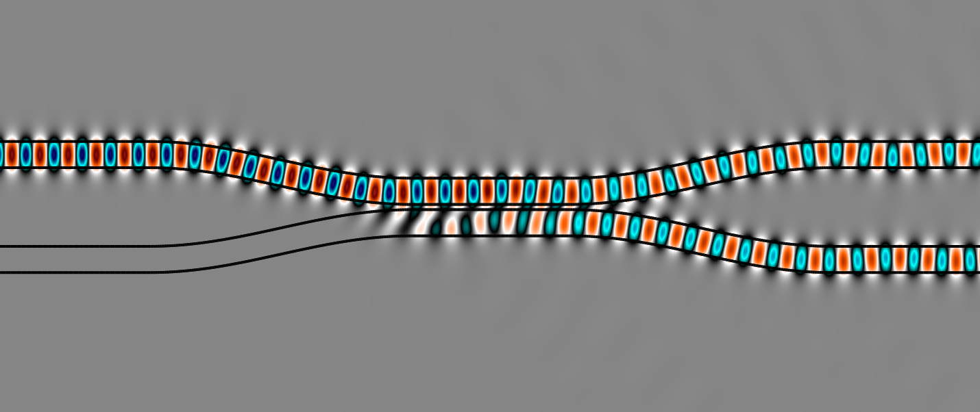
(a) COUPLER

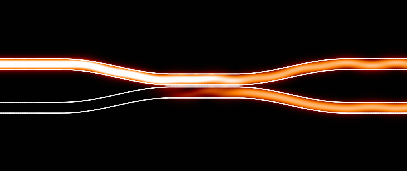
(b) COUPLER

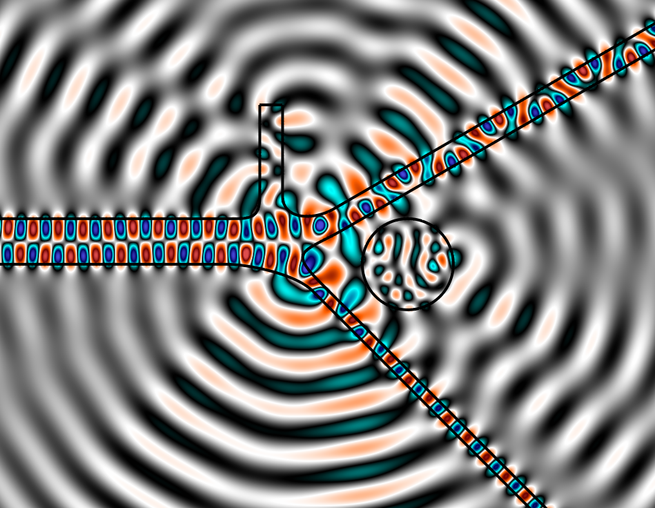
(c) BRANCH

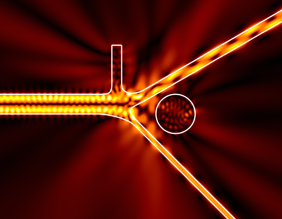
(d) BRANCH

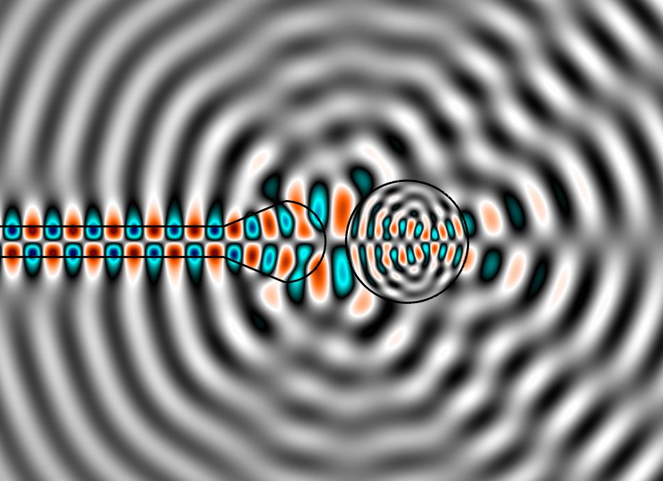
(e) HORN

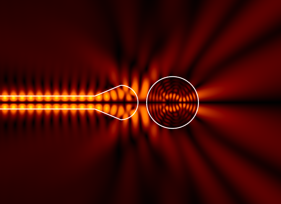
(f) HORN

(g) Colormap for $\text{Re}(u)$

(h) Colormap for $|u|$

Figure 3: Real part and absolute value of $u_{w}$ (left and right columns, respectively) produced by the WGF method for several open-waveguide problems.

4 Numerical examples

This section demonstrates the character of the WGF method introduced in Sec. 3 through a variety of numerical results. These results were obtained by means of a Matlab implementation of the algorithms described in Sec. 3.4 on a six-core 3.40 GHz Intel i7-4930K Processor with 12 Mb of cache and 32 Gb of RAM. As mentioned in Sec. 3.2, a Nyström method was utilized, where the number of points per wavelength was selected in such a way that the dominant error arises from the windowed truncation. The results in this paper were obtained by means of discretizations containing a number of eight to twelve points per wavelength, as needed to guarantee the accuracy reported for each numerical solution. The reported errors were evaluated by means of the expression

$$\displaystyle\text{Error}=\sqrt{\frac{\sum_{i=1}^{N_{d}}|u_{w}(\boldsymbol{r}_{i})-u^{\text{ref}}(\boldsymbol{r}_{i})|^{2}}{\sum_{i=1}^{N_{d}}|u^{\text{ref}}(\boldsymbol{r}_{i})|^{2}}}$$ (27)

with $N_{d}=100$, and where the $N_{d}$ points $\boldsymbol{r}_{i}$ lie along certain curves, selected in different manner for each test case, along which significant features of the numerically computed fields were observed. The errors in all the nonuniform waveguide problems were evaluated by means of equation (27) with reference solutions $u^{\text{ref}}$ produced by means of window functions $w_{A}$ with $A/\lambda>20$.

The first numerical example considered here is a simple uniform waveguide—for which, physically, a single mode (equation (5)), or even a superposition of such modes, can propagate from $-\infty$ to $+\infty$ without disturbance. This simple problem provides a direct test for the accuracy of the proposed WGF approach, for which errors were evaluated by using exact solutions as references: $u^{\text{ref}}=u$ in this case. The incident field was prescribed on the region $\Omega^{\text{inc}}=\{z\leq 0\}$. The observed error as a function of the window size is displayed in Fig. 2 under the label “FLAT”.

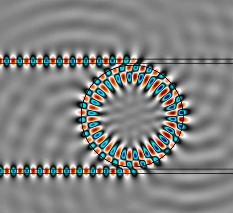
(a) DISK

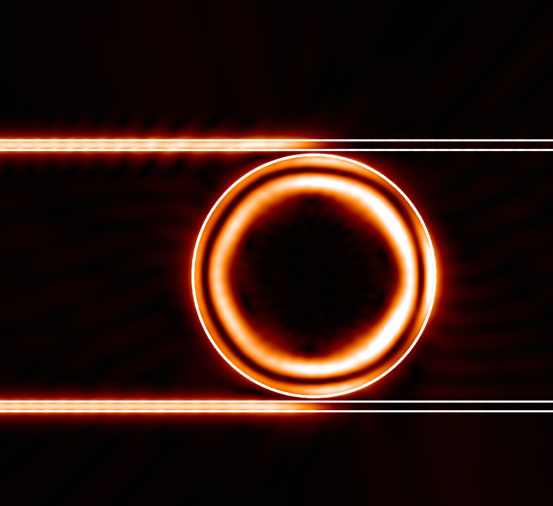
(b) DISK

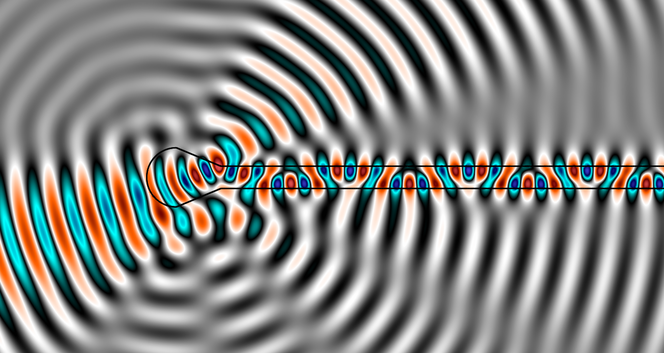
(c) ILLUM

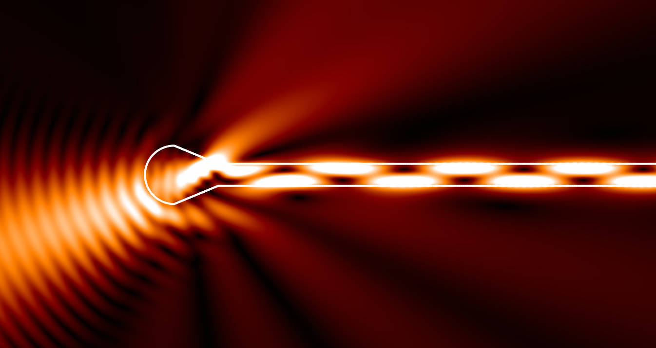
(d) ILLUM

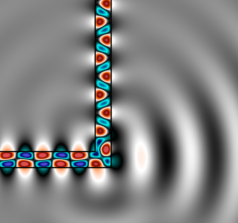
(e) L-BEND

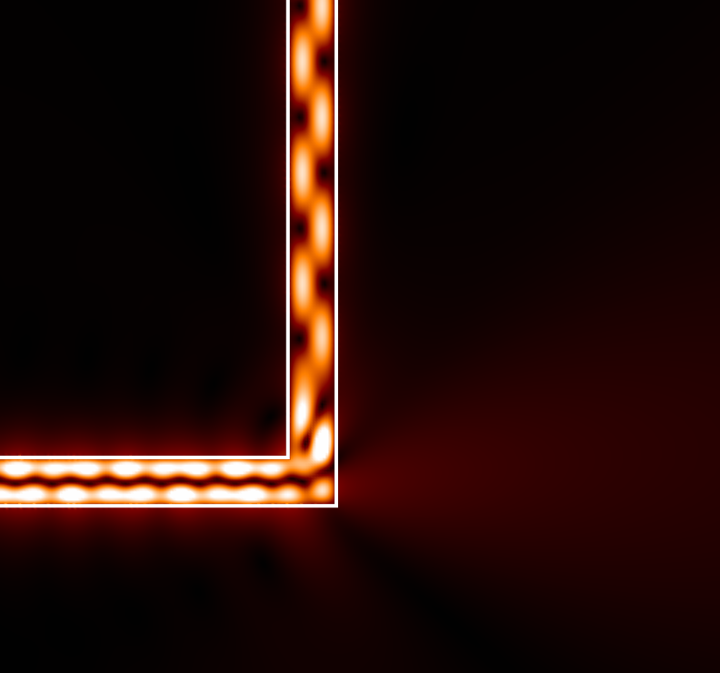
(f) L-BEND

(g) Colormap for $\text{Re}(u)$

(h) Colormap for $|u|$

Figure 4: Real part and absolute value of $u_{w}$ (left and right columns, respectively) produced by the WGF method for several open-waveguide problems.

Error curves for a number of additional configurations are also included in Fig. 2, and corresponding near field images are displayed in Figs. 3 and 4 . (The “trivial” near field image for the uniform waveguide mentioned above is not included in Figs. 3 and 4 .) The configurations considered (under TE or TM polarizations, as indicated in each case) are as follows:

• COUPLER (TE). Optical coupler illuminated by the first symmetric mode incoming from the top-left SIW. Waveguide core wavenumber $k_{\text{co}}=2\pi$, cladding wavenumber $k_{\text{cl}}=\pi$ and waveguide half-width $h=0.5$ were used. The waveguide separation in the cross-talk region was set to $0.2$.

• BRANCH (TE). Branching waveguide structure illuminated by the first antisymmetric mode incoming from the left SIW. The half-widths of the horizontal, top-right and bottom right SIWs are $1$, $0.5$ and $0.25$, respectively, and the angle between the two branching waveguides is $5\pi/12$ radians. The bottom-right SIW is a single-mode waveguide: only one specific mode can propagate along this structure. The wavenumbers in the core, cladding and circular obstacle regions are $k_{\text{co}}=2\pi$, $k_{\text{cl}}=\pi$ and $k_{\text{ob}}=5\pi/2$, respectively.

• HORN (TE). Terminated waveguide horn antenna illuminating a dielectric circular obstacle. The system is illuminated by the first antisymmetric mode of the waveguide. The core and cladding wavenumbers are $k_{\text{co}}=2\pi$ and $k_{\text{cl}}=4\pi/3$ respectively, and the circular obstacle wavenumber is $k_{\text{ob}}=4\pi$. The half-width of the waveguide is $h=0.5$ and the radius of the obstacle is $2$.

• DISK (TE). Circular disk resonator [19, Sec. 16.5]. The device is illuminated by the first symmetric mode incoming from the top-left waveguide. Both waveguides have core wavenumbers $k_{\text{co}}=250\pi/127$, the cladding wavenumber is $k_{\text{cl}}=125\pi/127$ and the disk has the same wavenumber as the core regions. The waveguide half-widths are both $h=0.2$, the disk has radius $5$, and separation between the waveguides and the disk is $0.2$. The wavenumbers were selected to excite a near resonance in the circular cavity.

• ILLUM (TE). Excitation of waveguide modes in a terminated waveguide. The structure is illuminated by a beam incoming from the left at an angle $\pi/10$ radians below the horizontal. (A description of the illuminating field is presented below.) The core and cladding wavenumbers are given by $k_{\text{co}}=2\pi$ and $k_{\text{cl}}=4\pi/3$ respectively, while the half-width of the waveguide is $h=0.5$.

• L-BEND (TM). Sharp $L-$bend illuminated by the first antisymmetric mode incoming from the left waveguide. The core and cladding wavenumbers are $k_{\text{co}}=2\pi$ and $k_{\text{cl}}=2\pi/3$ respectively, and the waveguide half-width is given by $h=0.5$.

The labels used here (COUPLER, BRANCH, etc.) correspond to those used in Figs. 2, 3, and 4. The computing times required to achieve an accuracy better than $1.0\times 10^{-6}$ are presented in Table 2.

The illuminating field used for the configuration ILLUM is given by the angular spectrum representation [11, Eq. (49)]

$$u^{\text{inc}}(r,\theta)=\int_{-\pi/2}^{\pi/2}F(\alpha)e^{ik_{1}r\cos{(\theta+\alpha)}}{d}\alpha,$$ (28)

with $F(\alpha)=e^{-12.5(\alpha+\pi/10)^{2}}$. Note that equation (16) does not directly apply in this case since the illuminating field used here is not a waveguide mode. But only slight modifications are necessary: the relevant equation in this case is

$$E(\boldsymbol{r})\boldsymbol{\phi}^{\text{scat}}(\boldsymbol{r})+T[\boldsymbol{\phi}^{\text{scat}}](\boldsymbol{r})=\boldsymbol{\phi}^{\text{inc}}(\boldsymbol{r}),\quad\boldsymbol{r}\in\Gamma.$$ (29)

This equation can be solved by a procedure analogous to that presented in Sec. 3.4.

Problem	#-Unknowns	$A/\lambda$	Time-$\boldsymbol{\phi}^{\text{scat}}$	Time-$u_{w}$
FLAT	1752	9	1.06	3.47
COUPLER	6450	12	13.05	9.23
BRANCH	5978	14	13.82	8.13
HORN	2902	15	3.28	7.69
DISK	6556	16	11.62	5.09
ILLLUM	1374	15	0.83	3.34
L-BEND	2516	12	2.03	3.80

Table 2: Computing times (in seconds) required by the WGF method to produce the densities $\boldsymbol{\phi}^{\text{scat}}$ (on the discretization grid) and to evaluate the fields $u_{w}$ (on a $128\times 128$ evaluation grid), with an accuracy better than $1.0\times 10^{-6}$, for the various test cases mentioned in the text.

5 Conclusions

The WGF method introduced in this paper provides super-algebraically accurate approximations as the window sizes $A$ are increased. The proposed approach retains the attractive qualities of boundary integral equation methods, such as reduced dimensionality, efficient parallelization and high-order accuracy for arbitrary geometries. And, while the present implementation is based on use of Nyström integral-equation solvers, any available boundary integral method for transmission problems, such as, e.g., those based on the Method of Moments, can be easily modified to incorporate the WGF methodology. The ideas presented here can be generalized to the three-dimensional case; such generalizations will be presented elsewhere.

References

- [1] J.-P. Berenger. A perfectly matched layer for the absorption of electromagnetic waves. Journal of Computational Physics, 114(2):185–200, Oct. 1994.
- [2] O. P. Bruno and B. Delourme. Rapidly convergent two-dimensional quasi-periodic Green function throughout the spectrum-including Wood anomalies. Journal of Computational Physics, 262:262–290, 2014.
- [3] O. P. Bruno, M. Lyon, C. Pérez-Arancibia, and C. Turc. Windowed Green Function Method for Layered-Media Scattering. SIAM Journal on Applied Mathematics, 76(5):1871–1898, Sept. 2016.
- [4] O. P. Bruno, S. P. Shipman, C. Turc, and S. Venakides. Superalgebraically convergent smoothly windowed lattice sums for doubly periodic green functions in three-dimensional space. Proceedings of the Royal Society of London A: Mathematical, Physical and Engineering Sciences, 472(2191), 2016.
- [5] J. Chaubell, O. P. Bruno, and C. O. Ao. Evaluation of em-wave propagation in fully three-dimensional atmospheric refractive index distributions. Radio Science, 44(1), 2009.
- [6] G. Ciraolo. Non-Rectilinear Waveguides: Analytical and Numerical Results Based on the Green’s Function. PhD thesis, Universita Degli Studi Di Firenze, 2005.
- [7] G. Ciraolo and R. Magnanini. Analytical results for 2-D non-rectilinear waveguides based on the Green’s function. Mathematical Methods in the Applied Sciences, 31(13):1–18, 2008.
- [8] D. Colton and R. Kress. Integral Equation Methods in Scattering Theory. 1983.
- [9] D. Colton and R. Kress. Inverse Acoustic and Electromagnetic Scattering Theory. Springer, New York, third edition, 2013.
- [10] L. Demanet and L. Ying. Scattering in flatland: efficient representations via wave atoms. Foundations of Computational Mathematics. The Journal of the Society for the Foundations of Computational Mathematics, 10(5):569–613, 2010.
- [11] J. DeSanto and P. A. Martin. On the derivation of boundary integral equations for scattering by an infinite one-dimensional rough surface. The Journal of the Acoustical Society of America, 102(1):67, 1997.
- [12] A. Farjadpour, D. Roundy, A. Rodriguez, M. Ibanescu, P. Bermel, J. D. Joannopoulos, S. G. Johnson, and G. W. Burr. Improving accuracy by subpixel smoothing in the finite-difference time domain. Optics Letters, 31(20):2972, Oct. 2006.
- [13] N. N. Lebedev. Special functions and their applications. Prentice-Hall, Inc., 1965.
- [14] R. Magnanini and F. Santosa. Wave Propagation in a 2-D Optical Waveguide. SIAM Journal on Applied Mathematics, 61(4):1237–1252, 2001.
- [15] J. A. Monro. A Super-Algebraically Convergent, Windowing-Based Approach to the Evaluation of Scattering from Periodic Rough Surfaces. PhD thesis, California Institute of Technology, 2007.
- [16] A. I. Nosich. Radiation conditions, limiting absorption principle, and general relations in open waveguide scattering. Journal of electromagnetic waves and applications, 8(3):329–353, 1994.
- [17] C. Perez-Arancibia. Windowed integral equation methods for problems of scattering by defects and obstacles in layered media. PhD thesis, California Institute of Technology, 2016.
- [18] S. Rao, D. Wilton, and A. Glisson. Electromagnetic scattering by surfaces of arbitrary shape. IEEE Transactions on Antennas and Propagation, 30(3):409–418, May 1982.
- [19] A. Taflove and S. C. Hagness. Computational Electrodynamics: The Finite-Difference Time-Domain Method. Artech House, Inc., third edition, 2005.
- [20] L. Zhang, J. H. Lee, A. Oskooi, A. Hochman, J. K. White, and S. G. Johnson. A Novel Boundary Element Method Using Surface Conductive Absorbers for Full-Wave Analysis of 3-D Nanophotonics. Journal of Lightwave Technology, 29(7):949–959, Apr. 2011.