Augmented Index and
Quantum Streaming Algorithms for Dyck(2) 

Abstract

We show how two recently developed quantum information theoretic tools can be applied to obtain lower bounds on quantum information complexity. We also develop new tools with potential for broader applicability, and use them to establish a lower bound on the quantum information complexity for the Augmented Index function on an easy distribution. This approach allows us to handle superpositions rather than distributions over inputs, the main technical challenge faced previously. By providing a quantum generalization of the argument of Jain and Nayak [IEEE TIT’14], we leverage this to obtain a lower bound on the space complexity of multi-pass, unidirectional quantum streaming algorithms for the Dyck(2) language.

1 Introduction

1.1 Streaming Algorithms and Augmented Index

The first bona fide quantum computers that are built are likely to involve a few hundred qubits, and be limited to short computations. This prompted much research into the capabilities of space bounded quantum computation, especially of quantum finite automata, during the early development of the theory of quantum computation (see, e.g., Refs. [MC00, KW97, AF98, ANTV02]). More recently, this has led to the investigation of quantum streaming algorithms [LG09, GKK⁺08, BCG14, Mon16].

Streaming algorithms were originally proposed as a means of processing massive real-world data that cannot be stored in their entirety in computer memory [Mut05]. Instead of random access to the input data, these algorithms receive the input in the form of a stream, i.e., one input symbol at a time. The algorithms attempt to solve some information processing task using as little space and time as possible, on occasion using more than one sequential pass over the input stream.

Streaming algorithms provide a natural framework for studying simple, small-space quantum computation beyond the scope of quantum finite automata. Some of the works mentioned above (e.g., LeGall [LG09]) show how quantum streaming algorithms can accomplish certain specially crafted tasks with exponentially smaller space, as compared with classical algorithms. This led Jain and Nayak [JN14] to ask how much more efficient such quantum algorithms could be for other, more natural problems. They focused on Dyck(2), a well-studied and important problem from formal language theory [CS63]. Dyck(2) consists of all well-formed expressions with two types of parenthesis, denoted below by $a,\overline{a}$ and $b,\overline{b}$, with the bar indicating a closing parenthesis. More formally, $\textsc{Dyck}(2)$ is the language over the alphabet $\Sigma=\left\{a,\overline{a},b,\overline{b}\right\}$ defined recursively as

$$\textsc{Dyck}(2)\quad=\quad\varepsilon+\bigl{(}a\cdot\textsc{Dyck}(2)\cdot\overline{a}+b\cdot\textsc{Dyck}(2)\cdot\overline{b}\bigr{)}\cdot\textsc{Dyck}(2)\enspace,$$

where $\varepsilon$ is the empty string, ‘$\cdot$’ indicates concatenation of strings (or subsets thereof) and ‘$+$’ denotes set union.

The related problem of recognizing whether a given expression with parentheses is well-formed was originally studied by Magniez, Mathieu, and Nayak [MMN14] in the context of classical streaming algorithms. They discovered a remarkable phenomenon, that providing bi-directional access to the input stream leads to an exponentially more space-efficient algorithm. They presented a randomized streaming algorithm that makes one pass over the input, uses ${\mathrm{O}}(\sqrt{n\log n}\,)$ bits, and makes polynomially small probability of error to determine membership of expressions of length ${\mathrm{O}}(n)$ in Dyck(2). Moreover, they proved that this space bound is optimal for error at most $1/(n\log n)$, and conjectured that a similar polynomial space bound holds for multi-pass algorithms as well. Magniez et al. complemented this with a second randomized algorithm that makes two passes in opposite directions over the input, uses only ${\mathrm{O}}(\log^{2}n)$ space, and has polynomially small probability of error. Later, two sets of authors [CCKM13, JN14] independently and concurrently proved the conjectured hardness of Dyck(2) for classical multi-pass streaming algorithms that read the input only in one direction. They showed that any unidirectional randomized $T$-pass streaming algorithm that recognizes length $n$ instances of Dyck(2) with a constant probability of error uses space $\Omega(\sqrt{n}/T)$.

The space lower bounds for Dyck(2) established in Refs. [MMN14, CCKM13, JN14] all rely on a connection with a two-party communication problem, Augmented Index, a variant of Index, a basic problem in two-party communication complexity. In the Index function problem, one party, Alice, is given a string $x\in\left\{0,1\right\}^{n}$, and the other party, Bob, is given an index $k\in[n]$, for some positive integer $n$. Their goal is to communicate with each other and compute $x_{k}$, the $k$th bit of the string $x$. In the Augmented Index function problem, Bob is given the prefix $x[1,k-1]$ (the first $k-1$ bits of $x$) and a bit $b$ in addition to the index $k$. The goal of the two parties is to determine if $x_{k}=b$ or not. The three works cited above (see also [CK11]) all prove information cost trade-offs for Augmented Index. As a result, in any bounded-error protocol for the function, either Alice reveals $\Omega(n)$ information about her input $x$, or Bob reveals $\Omega(1)$ information about the index $k$ (even under an easy distribution, the uniform distribution over zeros of the function).

Motivated by the abovementioned works, Jain and Nayak [JN14] studied quantum protocols for Augmented Index. They defined a notion of quantum information cost for distributions with a limited form of dependence, and then arrived at a similar tradeoff as in the classical case. This result, however, does not imply a lower bound on the space required by quantum streaming algorithms for Dyck(2). The issue is that the reduction from low information cost protocols for Augmented Index to small space streaming algorithms breaks down in the quantum case (for the notion of quantum information cost they proposed). This left open the possibility of more efficient unidirectional quantum streaming algorithms.

1.2 Overview of Results

We establish the following lower bound on the space complexity of $T$-pass, unidirectional quantum streaming algorithms for Dyck(2), thus solving the question posed by Jain and Nayak [JN14].

Theorem 1.1

For any $T\geq 1$, any unidirectional $T$-pass quantum streaming algorithm that recognizes $\textsc{Dyck}(2)$ with a constant probability of error uses space $\Omega(\sqrt{n}/T^{3})$ on length $n$ instances of the problem.

The space bound above holds for a general model for quantum streaming algorithms, one in which the computation is characterized by arbitrary quantum operations. In particular, the computation may be non-unitary, and may use “on-demand” ancillary qubits in addition to the allowed work space. Some earlier work showing strong limitations of bounded space, such as that on quantum finite automata [ANTV02], assumed unitary evolution.

Theorem 1.1 shows that, possibly up to logarithmic factors and the dependence on the number of passes, quantum streaming algorithms are no more efficient than classical ones for this problem. In particular, this provides the first natural example for which classical bi-directional streaming algorithms perform exponentially better than unidirectional quantum streaming algorithms.

Theorem 1.1 is a consequence of a lower bound that we establish on a measure of quantum information cost introduced by Touchette [Tou15]. (Henceforth, we use the term “quantum information cost” without any qualification to refer to this notion.) We consider this cost for any quantum protocol $\Pi$ computing the Augmented Index function, with respect to an “easy” distribution $\mu_{0}$: the uniform distribution over the zeros of the function. Due to the asymmetry of the Augmented Index function, we distinguish between the amount of information Alice transmits to Bob, denoted $\mathrm{QIC}_{{\mathrm{A}}\rightarrow{\mathrm{B}}}(\Pi,\mu_{0})$ and the amount of information Bob transmits to Alice, denoted $\mathrm{QIC}_{{\mathrm{B}}\rightarrow{\mathrm{A}}}(\Pi,\mu_{0})$; see Section 2.4 for formal definitions for these notions. Our main technical contributions are in proving the following trade-off.

Theorem 1.2

In any $t$-round quantum protocol $\Pi$ computing the Augmented Index function $f_{n}$ with constant error $\varepsilon\in[0,1/4)$ on any input, either $\mathrm{QIC}_{{\mathrm{A}}\rightarrow{\mathrm{B}}}(\Pi,\mu_{0})\in\Omega(n/t^{2})$ or $\mathrm{QIC}_{{\mathrm{B}}\rightarrow{\mathrm{A}}}(\Pi,\mu_{0})\in\Omega(1/t^{2})$.

A more precise statement is presented as Theorem 6.1. As in previous works, establishing a lower bound on the quantum information cost for such an easy distribution is necessary; the direct sum argument that links quantum streaming algorithms to quantum protocols for Augmented Index crucially hinges on this. (This phenomenon is common in such direct sum arguments.)

The high level intuition underlying the proof of Theorem 1.2 and its structure is the same as that in Ref. [JN14]. There are two principal challenges in their approach, and the choice of an appropriate measure of information cost is fundamental to overcoming both challenges. The first challenge is a direct sum argument that relates streaming algorithms for Dyck(2) and communication protocols for Augmented Index. The second challenge is establishing an information cost trade-off for Augmented Index. Jain and Nayak considered several notions of information cost, each one of which was effective in addressing one challenge but not the other. This was further complicated by the intrinsic correlation of the inputs for Augmented Index held by the two parties. Indeed, an important motivation behind the notion of quantum information cost used in Ref. [JN14] is the desire to avoid leaking information about the inputs by virtue of their preparation in superposition, instead of exchanging information through interaction alone. The notion they analyzed in detail admits an information cost trade-off, but not a connection between streaming algorithms and low information protocols. In particular, the notion does not seem to be bounded by communication complexity.

Quantum information cost, as proposed by Touchette [Tou15], turns out to be a suitable choice for quantifying the information content of messages in our context. It is defined in terms of conditional mutual information, conditioned on the recipient’s quantum state. Thus, this notion naturally avoids the difficulties arising from the intrinsic correlation between the two parties’ inputs. It is also relatively simple to derive low quantum information cost protocols for Augmented Index from small-space streaming algorithms for Dyck(2), through a direct sum argument. Remarkably, the properties of quantum information cost allow us to execute the reduction even for algorithms whose computation involves arbitrary quantum operations, including non-unitary evolution. However, a quantum information cost trade-off for Augmented Index still presents significant obstacles. In order to overcome these, we develop new tools for quantum communication complexity that we believe have broader applicability.

One tool is a generalization of the well-known Average Encoding Theorem of (classical and) quantum complexity theory [KNTZ07], which formalizes the intuition that weakly correlated systems are nearly independent. We call this generalized version the Superposition-Average Encoding Theorem, as it allows us to handle arbitrary superpositions over inputs to quantum communication protocols (as opposed to classical distributions over inputs). The proof of this theorem builds on the breakthrough result by Fawzi and Renner [FR15], linking conditional quantum mutual information to the optimal recovery map acting on the conditioning system. Note that there is an obvious generalization of the Average Encoding Theorem to an analogous result for conditional quantum mutual information implied by the Fawzi-Renner inequality together with the Uhlmann theorem. This cannot directly be used in a proof à la Ref. [JN14]. For one, such a generalization would give us a unitary operation that acts on one part of a (pure) “reconstructed” state, and maps it to a state close to a target state. The hybrid argument in Ref. [JN14] relies on the commutativity of such unitary operations corresponding to successive messages in a protocol, whereas the operations obtained by the obvious generalization do not commute.

Another key ingredient in the proof of Theorem 1.2 is a Quantum Cut-and-Paste Lemma, a variant of a technique used in Refs. [JRS03, JN14], that allows us to deal with easy distributions over inputs. The cut-and-paste lemma for randomized communication protocols connects the distance between transcripts obtained by running protocols on inputs chosen from a two-by-two rectangle $\{x,x^{\prime}\}\times\{y,y^{\prime}\}$. The cut-and-paste lemma is very powerful, and a direct quantum analogue does not hold. We can nevertheless obtain the following weaker variant, linking any four possible pairs of inputs in a two-by-two rectangle: if the states for a fixed input $y$ to Bob are close up to a local unitary operator on Alice’s side and the states for a fixed input $x$ to Alice are close up to a local unitary operator on Bob’s side, then, up to local unitary operators on Alice’s and Bob’s sides, the states for all pairs $(x^{\prime\prime},y^{\prime\prime})$ of inputs in the rectangle $\{x,x^{\prime}\}\times\{y,y^{\prime}\}$ are close to each other. This lemma allows us to link output states of protocols on inputs from an easy distribution, all mapping to the same output value, to an output state corresponding to a different output value. This helps derive a contradiction to the assumption of low quantum information cost, as states corresponding to different outputs are distinguishable with constant probability.

We go a step further with the quantum information cost trade-off. We provide an alternative way to achieve a similar result, by using a notion of information cost tailored to the Augmented Index problem. An important stepping stone in this approach is the recently developed Information Flow Lemma due to Laurière and Touchette [LT17a, LT17b]. The lemma allows us to track the transfer of information due to interaction in quantum protocols, and provides insight into how information might be leaked due to a superposition over inputs. By conditioning on a suitable classical register, we avoid such leakage of information. Pushing these ideas further, we are able to bring the Average Encoding Theorem to bear in this context as well. This helps us obtain a slightly better round-dependence in the information cost trade-off.

Organization.

Background and definitions related to quantum communication, information theory, and streaming algorithms are presented in Section 2. We then adapt, in Section 3, the known two-step reduction from Augmented Index to Dyck(2) to the new notion for information cost due to Touchette [Tou15] and to the general model for streaming algorithms that we define. The technical tools that we develop and use are presented in Section 4. The main lower bound on the quantum information cost of the Augmented Index function is derived in Section 5. A lower bound with a slightly better dependence on the number of rounds is presented in Section 6.

Acknowlegements.

We are grateful to Mark Braverman, Ankit Garg, Young Kun Ko, and Jieming Mao for useful discussions related to the development of the Superposition-Average Encoding Theorem and Quantum Cut-and-Paste Lemma.

2 Preliminaries

We refer the reader to text books such as [Wat18, Wil13] for standard concepts and the associated notation from quantum information.

2.1 Quantum Communication Complexity

We use the following notation for interactive communication between two parties, called Alice and Bob by convention. For a register $S$, we denote the set of its possible quantum states by $\mathcal{D}(S)$. An $M$-message protocol $\Pi$ for a task with input registers $A_{\mathrm{in}}B_{\mathrm{in}}$ and output registers $A_{\mathrm{out}}B_{\mathrm{out}}$ is defined by a sequence of isometries $U_{1},\dotsc,U_{M+1}$ along with a pure state $\psi\in\mathcal{D}(T^{\mathrm{A}}T^{\mathrm{B}})$ shared between Alice and Bob, for some arbitrary but finite dimensional registers $T^{\mathrm{A}}T^{\mathrm{B}}$. We refer to $\psi$ as the shared entanglement. We have $M+1$ isometries in an $M$-message protocol, as one isometry is applied before each message, and a final isometry is applied after the last message is received. We assume that Alice sends the first message. In the case of even $M$, the registers $A_{1},A_{3},\dotsc,A_{M-1},A^{\prime}$ are held by Alice, the registers $B_{2},B_{4},\dotsc,B_{M-2},B^{\prime}$ are held by Bob, and the registers $C_{1}C_{2}C_{3}\cdots C_{M}$ represent the quantum messages exchanged by Alice and Bob. The $M+1$ isometries act on these registers as indicated by the superscripts below (also see Figure 1):

$$U_{1}^{A_{\mathrm{in}}T^{\mathrm{A}}\rightarrow A_{1}C_{1}},\qquad U_{2}^{B_{\mathrm{in}}T^{\mathrm{B}}C_{1}\rightarrow B_{2}C_{2}},\qquad U_{3}^{A_{1}C_{2}\rightarrow A_{3}C_{3}},\qquad U_{4}^{B_{2}C_{3}\rightarrow B_{4}C_{4}},$$

$$\;\cdots,\qquad U_{M}^{B_{M-2}C_{M-1}\rightarrow B_{\mathrm{out}}B^{\prime}C_{M}},\qquad U_{M+1}^{A_{M-1}C_{M}\rightarrow A_{\mathrm{out}}A^{\prime}}\enspace.$$

We adopt the convention that, at the outset, $A_{0}=A_{\mathrm{in}}T^{\mathrm{A}}$, $B_{0}=B_{\mathrm{in}}T^{\mathrm{B}}$; for odd $i$ with $1\leq i<M$, $B_{i}=B_{i-1}$; for even $i$ with $1<i\leq M$, $A_{i}=A_{i-1}$; also $B_{M}=B_{M+1}=B_{\mathrm{out}}B^{\prime}$, and $A_{M+1}=A_{\mathrm{out}}A^{\prime}$. In this way, after the application of $U_{i}$, Alice holds register $A_{i}$, Bob holds register $B_{i}$ and the communication register is $C_{i}$. In the case of an odd number of messages $M$, the registers corresponding to $U_{M},U_{M+1}$ are changed appropriately. We slightly abuse notation and also write $\Pi$ to denote the channel from $A_{\mathrm{in}}B_{\mathrm{in}}$ to $A_{\mathrm{out}}B_{\mathrm{out}}$ implemented by the protocol. That is, for any $\rho\in\mathcal{D}(A_{\mathrm{in}}B_{\mathrm{in}})$,

$$\Pi(\rho)\quad\coloneqq\quad\mathop{{\mathrm{Tr}}_{A^{\prime}B^{\prime}}}\left[U_{M+1}U_{M}\cdots U_{2}U_{1}(\rho\otimes\psi)\right]\,.$$

The registers $A^{\prime}$ and $B^{\prime}$ that are discarded by Alice and Bob, respectively, are two of the registers at the end of the protocol. As on the RHS above, we sometimes omit the superscript if the system is clear from context.

We restrict our attention to protocols with classical inputs $XY$, with $A_{\mathrm{in}}B_{\mathrm{in}}$ initialized to $XY$, and to so-called “safe protocols”. Safe protocols only use $A_{\mathrm{in}}B_{\mathrm{in}}$ as control registers. As explained in Section 2.4, this does not affect the results presented in this article.

We imagine that the joint classical input $XY$ is purified by a register $R$. We often partition the purifying register as $R=R_{X}R_{Y}$, indicating that the classical input $XY$, distributed as $\nu$, and represented by the quantum state $\rho_{\nu}$,

$$\rho_{\nu}^{XY}\quad\coloneqq\quad\sum_{x,y}\nu(x,y)\;\left|x\right\rangle\!\left\langle x\right|^{X}\otimes\left|y\right\rangle\!\left\langle y\right|^{Y}\enspace,$$

is purified as

$$\mathop{\left|\rho_{\nu}\right>}\nolimits\quad\coloneqq\quad\sum_{x,y}\sqrt{\nu(x,y)}\;\mathop{\left|xxyy\right>}\nolimits^{XR_{X}YR_{Y}}\enspace.$$

We also use other partitions more appropriate for our purposes, corresponding to particular preparations of the inputs $X$ and $Y$.

We define the quantum communication cost of $\Pi$ from Alice to Bob as

$${\mathrm{QCC}}_{{\mathrm{A}}\to{\mathrm{B}}}(\Pi)\quad\coloneqq\quad\sum_{i\in[0,(M-1)/2]}\log\left|C_{2i+1}\right|\,,$$

and the quantum communication cost of $\Pi$ from Bob to Alice as

$${\mathrm{QCC}}_{{\mathrm{B}}\to{\mathrm{A}}}(\Pi)\quad\coloneqq\quad\sum_{i\in[1,M/2]}\log\left|C_{2i}\right|\,,$$

where for a register $D$, the notation $\left|D\right|$ stands for the dimension of the state space associated with the register. The total communication cost of the protocol is then the sum of these two quantities.

\begin{overpic}[width=433.62pt]{int_prot_no_label.pdf} \put(0.0,65.0){Reference} \put(0.0,45.0){Alice} \put(0.0,22.0){Bob} \put(6.0,31.0){\footnotesize$\mathop{\left|\rho_{\nu}\right>}\nolimits$} \put(15.0,66.5){\footnotesize$R$} \put(15.0,54.0){\footnotesize$A_{{\mathrm{in}}}$} \put(15.0,13.8){\footnotesize$B_{{\mathrm{in}}}$} \put(15.0,44.0){\footnotesize$T^{\mathrm{A}}$} \put(15.0,19.0){\footnotesize$T^{\mathrm{B}}$} \put(22.1,49.5){\footnotesize$U_{1}$} \put(15.0,31.0){\footnotesize$\mathop{\left|\psi\right>}\nolimits$} \put(26.2,54.0){\footnotesize$A_{1}$} \put(26.2,48.0){\footnotesize$C_{1}$} \put(33.0,15.5){\footnotesize$U_{2}$} \put(37.2,54.0){\footnotesize$A_{2}$} \put(37.2,17.4){\footnotesize$C_{2}$} \put(37.2,13.7){\footnotesize$B_{2}$} \put(44.2,49.5){\footnotesize$U_{3}$} \put(48.2,54.0){\footnotesize$A_{3}$} \put(48.2,48.0){\footnotesize$C_{3}$} \put(48.2,13.7){\footnotesize$B_{3}$} \put(55.0,33.0){\footnotesize$\cdots$} \put(59.5,54.0){\footnotesize$A_{M-1}$} \put(59.5,48.0){\footnotesize$C_{M-1}$} \put(59.5,13.7){\footnotesize$B_{M-1}$} \put(66.5,15.5){\footnotesize$U_{M}$} \put(71.7,54.0){\footnotesize$A_{M}$} \put(73.5,23.0){\footnotesize$C_{M}$} \put(73.5,17.0){\footnotesize$B_{{\mathrm{out}}}$} \put(73.5,12.0){\footnotesize$B^{\prime}$} \put(75.9,49.5){\footnotesize$U_{M+1}$} \put(82.3,54.0){\footnotesize$A^{\prime}$} \put(82.3,50.9){\footnotesize$A_{{\mathrm{out}}}$} \put(92.0,33.0){\footnotesize$\Pi(\rho_{\nu})$} \end{overpic}

Figure 1: Depiction of an interactive quantum protocol, adapted from Ref. [Tou14, Figure 1], the full version of Ref. [Tou15].

2.2 Distance Measures

In order to distinguish between quantum states, we use two related distance measures: trace distance and Bures distance.

Trace Distance.

The trace distance between two quantum states $\rho$ and $\sigma$ in the same state space is denoted as $\|\rho-\sigma\|_{1}$ , where

$$\|O\|_{1}\quad\coloneqq\quad\mathop{{\mathrm{Tr}}}\left((O^{\dagger}O)^{\tfrac{1}{2}}\right)$$

is the trace norm for operators. In operational terms, the trace distance between the two states $\rho$ and $\sigma$ is four times the best possible bias with which we can distinguish between the two states, given a single copy of an unknown state out of the two.

We use the following properties of trace distance. First, it is a metric, so it is symmetric in $\rho,\sigma$, non-negative, evaluates to $0$ if and only if $\rho=\sigma$, and it satisfies the triangle inequality. Moreover, it is monotone under the action of channels: for any $\rho_{1},\rho_{2}\in\mathcal{D}(A)$ and channel $\mathcal{N}^{A\rightarrow B}$ from system $A$ to system $B$,

$$\|\mathcal{N}(\rho_{1})-\mathcal{N}(\rho_{2})\|_{1}\quad\leq\quad\|\rho_{1}-\rho_{2}\|_{1}\enspace.$$

For isometries, the inequality is tight, a property called isometric invariance of the trace distance. Hence, for any $\rho_{1}$, $\rho_{2}\in\mathcal{D}(A)$ and any isometry $U^{A\rightarrow B}$, we have

$$\|U(\rho_{1})-U(\rho_{2})\|_{1}\quad=\quad\|\rho_{1}-\rho_{2}\|_{1}\enspace.$$

Trace distance obeys a joint linearity property: for a classical system $X$ and two states

$$\begin{split}\rho_{1}^{XA}&\quad\coloneqq\quad\sum_{x}p_{X}(x)\,\left|x\right\rangle\!\left\langle x\right|^{X}\otimes\rho_{1,x}^{A}\enspace,\qquad\text{and}\\ \rho_{2}^{XA}&\quad\coloneqq\quad\sum_{x}p_{X}(x)\,\left|x\right\rangle\!\left\langle x\right|^{X}\otimes\rho_{2,x}^{A}\enspace,\end{split}$$ (2.1)

we have

$$\|\rho_{1}-\rho_{2}\|_{1}\quad=\quad\sum_{x}p_{X}(x)\;\|\rho_{1,x}-\rho_{2,x}\|_{1}\enspace.$$ (2.2)

Bures Distance.

Bures distance $\operatorname{{\mathfrak{h}}}$ is a fidelity based distance measure, defined for $\rho,\sigma\in\mathcal{D}(A)$ as

$$\operatorname{{\mathfrak{h}}}\!\left(\rho,\sigma\right)\quad\coloneqq\quad\sqrt{1-{\mathrm{F}}(\rho,\sigma)}\ ,$$

where fidelity ${\mathrm{F}}$ is defined as ${\mathrm{F}}(\rho,\sigma)\coloneqq\|\sqrt{\rho}\sqrt{\sigma}\|_{1}$.

We use the following properties of Bures distance. First, it is a metric, so it is symmetric in $\rho,\sigma$, non-negative, evaluates to $0$ if and only if $\rho=\sigma$, and satisfies the triangle inequality. Moreover, it is monotone under the action of a channel: for any $\rho_{1}$, $\rho_{2}\in\mathcal{D}(A)$ and quantum channel $\mathcal{N}^{A\rightarrow B}$,

$$\operatorname{{\mathfrak{h}}}\!\left(\mathcal{N}(\rho_{1}),\mathcal{N}(\rho_{2})\right)\quad\leq\quad\operatorname{{\mathfrak{h}}}\!\left(\rho_{1},\rho_{2}\right)\enspace.$$

For isometries, the inequality is tight, a property called isometric invariance of the Bures distance.

It is sometimes convenient to work with the square of the Bures distance. In particular, the square obeys a joint linearity property: for a classical system $X$ and two states $\rho_{1}^{XA},\rho_{2}^{XA}$ defined as in Eq. (2.1),

$$\operatorname{{\mathfrak{h}}}^{2}\!\left(\rho_{1},\rho_{2}\right)\quad=\quad\sum_{x}p_{X}(x)\,\operatorname{{\mathfrak{h}}}^{2}\!\left(\rho_{1,x},\rho_{2,x}\right)\enspace.$$ (2.3)

It also satisfies a weaker version of the triangle inequality: for any $\rho_{1}$, $\rho_{2}$ and $\sigma\in\mathcal{D}(A)$,

$$\operatorname{{\mathfrak{h}}}^{2}\!\left(\rho_{1},\rho_{2}\right)\quad\leq\quad 2\operatorname{{\mathfrak{h}}}^{2}\!\left(\rho_{1},\sigma\right)+2\operatorname{{\mathfrak{h}}}^{2}\!\left(\sigma,\rho_{2}\right)\enspace.$$ (2.4)

Local Transition Lemma.

The following lemma, a direct consequence of the Uhlmann theorem, is called the local transition lemma [KNTZ07], especially when expressed in terms of other metrics.

Lemma 2.1

Let $\rho_{1}$, $\rho_{2}\in\mathcal{D}(A)$ have purifications $\rho_{1}^{AR_{1}}$, $\rho_{2}^{AR_{2}}$, with $|R_{1}|\leq|R_{2}|$. Then, there exists an isometry $V^{R_{1}\rightarrow R_{2}}$ such that

$$\operatorname{{\mathfrak{h}}}\big{(}\rho_{1}^{A},\rho_{2}^{A}\big{)}\quad=\quad\operatorname{{\mathfrak{h}}}\Big{(}V\big{(}\rho_{1}^{AR_{1}}\big{)},\rho_{2}^{AR_{2}}\Big{)}\ .$$

Bures distance is related to trace distance through a generalization of the Fuchs-van de Graaf inequalities [FvdG99]: for any $\rho_{1}$, $\rho_{2}\in\mathcal{D}(A)$ , it holds that

$$\operatorname{{\mathfrak{h}}}^{2}\!\left(\rho_{1},\rho_{2}\right)\quad\leq\quad\frac{1}{2}\;\|\rho_{1}-\rho_{2}\|_{1}\quad\leq\quad\sqrt{2}\operatorname{{\mathfrak{h}}}\!\left(\rho_{1},\rho_{2}\right)\enspace.$$ (2.5)

2.3 Information Measures

In order to quantify the information content of a quantum state, we use a basic measure, von Neumann entropy, defined as

$${\mathrm{H}}(A)_{\rho}\quad\coloneqq\quad-\mathop{{\mathrm{Tr}}}\left(\rho\log\rho\right)$$

for any state $\rho\in\mathcal{D}(A)$. Here, we follow the convention that $0\log 0=0$, which is justified by a continuity argument. The logarithm is in base $2$. Note that ${\mathrm{H}}$ is invariant under isometries applied on $\rho$. If the state in question is clear from the context, we may omit the subscript. We also note that if system $A$ is classical, then von Neumann entropy reduces to Shannon entropy.

For a state $\rho^{ABC}\in\mathcal{D}(ABC)$, the mutual information between registers $A,B$ is defined as

$$\operatorname{{\mathrm{I}}}(A\!:\!B)_{\rho}\quad\coloneqq\quad{\mathrm{H}}(A)+{\mathrm{H}}(B)-{\mathrm{H}}(AB)\enspace,$$

and the conditional mutual information between them, given $C$, as

$$\operatorname{{\mathrm{I}}}(A\!:\!B\,|\,C)_{\rho}\quad\coloneqq\quad\operatorname{{\mathrm{I}}}(A\!:\!BC)-\operatorname{{\mathrm{I}}}(A\!:\!C)\enspace.$$

If $X$ is a classical system, $\operatorname{{\mathrm{I}}}(X\!:\!B)$ is also called the Holevo information.

Mutual information and conditional mutual information are symmetric in $A,B$, and invariant under a local isometry applied to $A,B$ or $C$. Since all purifications of a state are equivalent up to an isometry on the purification registers, we have that for any two pure states $\mathop{\left|\phi\right>}\nolimits^{ABCR^{\prime}}$ and $\mathop{\left|\psi\right>}\nolimits^{ABCR}$ such that $\phi^{ABC}=\psi^{ABC}$,

$$\operatorname{{\mathrm{I}}}(C\!:\!R^{\prime}\,|\,B)_{\phi}\quad=\quad\operatorname{{\mathrm{I}}}(C\!:\!R\,|\,B)_{\psi}\enspace.$$

For any state $\rho\in\mathcal{D}(ABC)$, we have the bounds

$$0\quad\leq\quad{\mathrm{H}}(A)\quad\leq\quad\log|A|\enspace,$$

$$0\quad\leq\quad\operatorname{{\mathrm{I}}}(A\!:\!B\,|\,C)\quad\leq\quad 2\;{\mathrm{H}}(A)\enspace.$$

For a multipartite quantum system $ABCD$, conditional mutual information satisfies a chain rule: for any $\rho\in\mathcal{D}(ABCD)$,

$$\operatorname{{\mathrm{I}}}(AB\!:\!C\,|\,D)\quad=\quad\operatorname{{\mathrm{I}}}(A\!:\!C\,|\,D)+\operatorname{{\mathrm{I}}}(B\!:\!C\,|\,AD)\enspace.$$

For any product state $\rho^{A_{1}B_{1}A_{2}B_{2}}\coloneqq\rho_{1}^{A_{1}B_{1}}\otimes\rho_{2}^{A_{2}B_{2}}$, entropy is additive across the bi-partition, so that, for example,

$${\mathrm{H}}(A_{1}A_{2})\quad=\quad{\mathrm{H}}(A_{1})+{\mathrm{H}}(A_{2})\enspace,$$

and the conditional mutual information between product systems vanishes:

$$\operatorname{{\mathrm{I}}}(A_{1}\!:\!A_{2}\,|\,B_{1}B_{2})\quad=\quad 0\enspace.$$

Two important properties of the conditional mutual information are non-negativity and the data processing inequality, both equivalent to a deep result in quantum information theory known as strong subadditivity [LR73]. For any state $\rho\in\mathcal{D}(ABC)$, channel $\mathcal{N}^{B\rightarrow B^{\prime}}$, and state $\sigma\coloneqq\mathcal{N}(\rho)$, we have

$$\operatorname{{\mathrm{I}}}(A\!:\!B\,|\,C)_{\rho} \quad\geq\quad 0,$$

$$\operatorname{{\mathrm{I}}}(A\!:\!B\,|\,C)_{\rho} \quad\geq\quad\operatorname{{\mathrm{I}}}(A\!:\!B^{\prime}\,|\,C)_{\sigma}\enspace.$$

For classical systems, conditioning is equivalent to taking an average: for any state

$$\rho^{ABCX}\quad\coloneqq\quad\sum_{x}p_{X}(x)\,\left|x\right\rangle\!\left\langle x\right|^{X}\otimes\rho_{x}^{ABC}$$

with a classical system $X$ and some states $\rho_{x}\in\mathcal{D}(ABC)$,

$$\operatorname{{\mathrm{I}}}(A\!:\!B\,|\,CX)_{\rho} \quad=\quad\sum_{x}p_{X}(x)\operatorname{{\mathrm{I}}}(A\!:\!B\,|\,C)_{\rho_{x}}\enspace.$$

Average Encoding Theorem.

The following lemma, known as the Average Encoding Theorem [KNTZ07, JRS03], formalizes the intuition that if a classical and a quantum registers are weakly correlated, then they are nearly independent.

Lemma 2.2

For any $\rho^{XA}\coloneqq\sum_{x}p_{X}(x)\,\left|x\right\rangle\!\left\langle x\right|^{X}\otimes\rho_{x}^{A}$ with a classical system $X$ and states $\rho_{x}\in\mathcal{D}(A)$,

$$\sum_{x}p_{X}(x)\operatorname{{\mathfrak{h}}}^{2}\!\left(\rho_{x}^{A},\rho^{A}\right) \quad\leq\quad\operatorname{{\mathrm{I}}}(X\!:\!A)_{\rho}\enspace.$$

Fawzi-Renner inequality.

We use the following breakthrough result by Fawzi and Renner [FR15]. It provides a lower bound on the quantum conditional mutual information in terms of the fidelity for the optimal recovery map.

Lemma 2.3

For any tripartite quantum state $\rho^{ACR}$, there exists a recovery map $\mathcal{R}^{A\rightarrow AC}$ from register $A$ to registers $AC$ satisfying

$$\operatorname{{\mathrm{I}}}(C\!:\!R\,|\,A)\quad\geq\quad-2\,\log_{2}{\mathrm{F}}(\rho^{ACR},\mathcal{R}(\rho^{AR}))\enspace.$$

In particular, it follows that

$$\operatorname{{\mathrm{I}}}(C\!:\!R\,|\,A)\quad\geq\quad\operatorname{{\mathfrak{h}}}^{2}\!\left(\rho^{ACR},\mathcal{R}(\rho^{AR})\right)\enspace.$$

2.4 Quantum Information Complexity

We rely on the notion of quantum information cost of a two-party communication protocol introduced by Touchette [Tou15]. We follow the notation and conventions associated with a two-party quantum communication protocol introduced in Section 2.1, and restrict ourselves to protocols with classical inputs $XY$ distributed as $\nu$.

Quantum information cost is defined in terms of the purifying register $R$, but is independent of the choice of purification. Given the asymmetric nature of the Augmented Index function, we consider the quantum information cost of messages from Alice to Bob and the ones from Bob to Alice separately. Such an asymmetric notion of quantum information cost was previously considered in Refs. [KLGR16, LT17a, LT17b].

Definition 2.4

Given a quantum protocol $\Pi$ with classical inputs distributed as $\nu$, the quantum information cost (of the messages) from Alice to Bob is defined as

$$\mathrm{QIC}_{{\mathrm{A}}\rightarrow{\mathrm{B}}}(\Pi,\nu)\quad\coloneqq\quad \sum_{i~{}\mathrm{odd}}\operatorname{{\mathrm{I}}}(R\!:\!C_{i}\,|\,B_{i})\enspace,$$

and the quantum information cost (of the messages) from Bob to Alice is defined as

$$\mathrm{QIC}_{{\mathrm{B}}\rightarrow{\mathrm{A}}}(\Pi,\nu)\quad\coloneqq\quad \sum_{i~{}\mathrm{even}}\operatorname{{\mathrm{I}}}(R\!:\!C_{i}\,|\,A_{i})\enspace.$$

It is immediate that quantum information cost is bounded above by quantum communication.

Remark 2.5

For any quantum protocol $\Pi$ with classical inputs distributed as $\nu$, the following hold:

$$\mathrm{QIC}_{{\mathrm{A}}\rightarrow{\mathrm{B}}}(\Pi,\nu) \quad\leq\quad 2\;{\mathrm{QCC}}_{A\rightarrow B}(\Pi)\enspace,\qquad\text{and}$$

$$\mathrm{QIC}_{{\mathrm{B}}\rightarrow{\mathrm{A}}}(\Pi,\nu) \quad\leq\quad 2\;{\mathrm{QCC}}_{B\rightarrow A}(\Pi)\enspace.$$

As a result, we may bound quantum communication complexity of a protocol from below by analysing its information cost.

We further restrict ourselves to “safe protocols”, in which the registers $A_{\mathrm{in}},B_{\mathrm{in}}$ are only used as control registers in the local isometries. This restriction does not affect the results in this article, for the following reason. Let $\Pi$ be any protocol with classical inputs distributed as $\nu$, in which the two parties may apply arbitrary isometries to their quantum registers. In particular, these registers include $A_{\mathrm{in}},B_{\mathrm{in}}$ which are initialized to the input. Let $\Pi^{\prime}$ be the protocol with the same registers as $\Pi$ and two additional quantum registers $A^{\prime}_{\mathrm{in}},B^{\prime}_{\mathrm{in}}$ of the same sizes as $A_{\mathrm{in}},B_{\mathrm{in}}\,$, respectively. In the protocol $\Pi^{\prime}$, the two parties each make a coherent local copy of their inputs into $A^{\prime}_{\mathrm{in}},B^{\prime}_{\mathrm{in}}\,$, respectively, at the outset. That is, Alice applies an isometry that maps

$$\mathop{\left|x\right>}\nolimits^{A_{\mathrm{in}}}\quad\mapsto\quad\mathop{\left|x\right>}\nolimits^{A^{\prime}_{\mathrm{in}}}\mathop{\left|x\right>}\nolimits^{A_{\mathrm{in}}}\enspace,$$

for each possible classical input $x$, and Bob applies a similar isometry to $B_{\mathrm{in}}$. The registers $A^{\prime}_{\mathrm{in}},B^{\prime}_{\mathrm{in}}$ are never touched hereafter, and the two parties simulate the original protocol $\Pi$ on the remaining registers. As Laurière and Touchette [LT17b, Proposition 9] show, the quantum information cost of $\Pi$ is at least as much as that of the protocol $\Pi^{\prime}$:

$$\mathrm{QIC}_{{\mathrm{A}}\rightarrow{\mathrm{B}}}(\Pi^{\prime},\nu)\quad \leq\quad\mathrm{QIC}_{{\mathrm{A}}\rightarrow{\mathrm{B}}}(\Pi,\nu)\enspace,\qquad\textrm{and}$$

$$\mathrm{QIC}_{{\mathrm{B}}\rightarrow{\mathrm{A}}}(\Pi^{\prime},\nu)\quad \leq\quad\mathrm{QIC}_{{\mathrm{B}}\rightarrow{\mathrm{A}}}(\Pi,\nu)\enspace.$$

Thus, the quantum information cost trade-off we show for safe protocols holds for arbitrary protocols as well.

We use another result due to Laurière and Touchette [LT17a, LT17b]. The result states that the total gain in (conditional) information by a party over all the messages is precisely the net (conditional) information gain at the end of the protocol. It allows us to keep track of the flow of information during interactive quantum protocols. For completeness, a proof is provided in Appendix B.

Lemma 2.6 (Information Flow Lemma)

Given a protocol $\Pi$, an input state $\rho$ with purifying register $R$ with arbitrary decompositions $R=R_{a}^{\mathrm{A}}R_{b}^{\mathrm{A}}R_{c}^{\mathrm{A}}=R_{a}^{\mathrm{B}}R_{b}^{\mathrm{B}}R_{c}^{\mathrm{B}}$, the following hold:

$$\sum_{i\geq 0}\operatorname{{\mathrm{I}}}(R_{a}^{\mathrm{B}}\!:\!C_{2i+1}\,|\,R_{b}^{\mathrm{B}}B_{2i+1})-\sum_{i\geq 1}\operatorname{{\mathrm{I}}}(R_{a}^{\mathrm{B}}\!:\!C_{2i}\,|\,R_{b}^{\mathrm{B}}B_{2i})\qquad$$

$$=\quad\operatorname{{\mathrm{I}}}(R_{a}^{\mathrm{B}}\!:\!B_{{\mathrm{out}}}B^{\prime}\,|\,R_{b}^{\mathrm{B}})-\operatorname{{\mathrm{I}}}(R_{a}^{\mathrm{B}}\!:\!B_{{\mathrm{in}}}\,|\,R_{b}^{\mathrm{B}})\enspace,\quad\textrm{and}$$

$$\sum_{i\geq 0}\operatorname{{\mathrm{I}}}(R_{a}^{\mathrm{A}}\!:\!C_{2i+2}\,|\,R_{b}^{\mathrm{A}}A_{2i+2})-\sum_{i\geq 0}\operatorname{{\mathrm{I}}}(R_{a}^{\mathrm{A}}\!:\!C_{2i+1}\,|\,R_{b}^{\mathrm{A}}A_{2i+1})$$

$$=\quad\operatorname{{\mathrm{I}}}(R_{a}^{\mathrm{A}}\!:\!A_{{\mathrm{out}}}A^{\prime}\,|\,R_{b}^{\mathrm{A}})-\operatorname{{\mathrm{I}}}(R_{a}^{\mathrm{A}}\!:\!A_{{\mathrm{in}}}\,|\,R_{b}^{\mathrm{A}})\enspace.$$

2.5 Quantum Streaming Algorithms

We refer the reader to the text [Mut05] for an introduction to classical streaming algorithms. Quantum streaming algorithms are similarly defined, with restricted access to the input, and with limited workspace.

In more detail, an input $x\in\Sigma^{n}\,$, where $\Sigma$ is some alphabet, arrives as a data stream, i.e., letter by letter in the order $x_{1},x_{2},\dotsc,x_{n}$. An algorithm is said to make a pass on the input, when it reads the data stream once in this order, processing it as described next. For an integer $T\geq 1$, a $T$-pass (unidirectional) quantum streaming algorithm ${\mathcal{A}}$ with space $s(n)$ and time $t(n)$ is a collection of quantum channels $\left\{{\mathcal{A}}_{i\sigma}:i\in[T],\sigma\in\Sigma\right\}$. Each operator ${\mathcal{A}}_{i\sigma}$ is a channel defined on a register of $s(n)$-qubits, and can be implemented by a uniform family of circuits of size at most $t(n)$. On input stream $x\in\Sigma^{n}\,$,

1. The algorithm starts with a register $W$ of $s(n)$ qubits, all initialized to a fixed state, say $\mathop{\left|0\right>}\nolimits$.

2. ${\mathcal{A}}$ performs $T$ sequential passes, $i=1,\dotsc,T$, on $x$ in the order $x_{1},x_{2},\dotsc,x_{n}$.

3. In the $i$th pass, when symbol $\sigma$ is read, channel ${\mathcal{A}}_{i\sigma}$ is applied to $W$.

4. The output of the algorithm is the state in a designated sub-register $W_{\mathrm{out}}$ of $W$, at the end of the $T$ passes.

We may allow for some pre-processing before the input is read, and some post-processing at the end of the $T$ passes, each with time complexity different from $t(n)$. As our work applies to streaming algorithms with any time complexity, we do not consider this refinement.

The probability of correctness of a streaming algorithm is defined in the standard way. If we wish to compute a family of Boolean functions $g_{n}:\Sigma^{n}\rightarrow\left\{0,1\right\}$, the output register $W_{\mathrm{out}}$ consists of a single qubit. On input $x$, let ${\mathcal{A}}(x)$ denote the random variable corresponding to the outcome when the output register is measured in the standard basis. We say ${\mathcal{A}}$ computes $g_{n}$ with (worst-case) error $\varepsilon\in[0,1/2]$ if for all $x$, $\Pr[{\mathcal{A}}(x)=g_{n}(x)]\geq 1-\varepsilon$.

In general, the implementation of a quantum channel used by a streaming algorithm with unitary operations involves one-time use of ancillary qubits (initialized to a fixed, known quantum state, say $\mathop{\left|0\right>}\nolimits$). These ancillary qubits are in addition to the $s(n)$-qubit register that is maintained by the algorithm. Fresh qubits may be an expensive resource in practice, for example, in NMR implementations, and one may argue that they be included in the space complexity of the algorithm. The lack of ancillary qubits severely restricts the kind of computations space-bounded algorithms can perform; see, for example, Ref. [ANTV02]. We choose the definition above so as to present the results we derive in the strongest possible model. Thus, the results also apply to implementations in which the “flying qubits” needed for implementing non-unitary quantum channels are relatively easy to prepare.

In the same vein, we may provide a quantum streaming algorithm arbitrary read-only access to a sequence of random bits. In other words, we may also provide the algorithm with a register $S$ of size at most $nTt(n)$ initialized to random bits from some distribution. Each quantum channel ${\mathcal{A}}_{i\sigma}$ now operates on registers $SW$, while using $S$ only as a control register. The bounds we prove hold in this model as well.

3 Reduction from Augmented Index to Dyck(2)

The connection between low-information protocols for Augmented Index and streaming algorithms for Dyck(2) contains two steps. The first is a reduction from an intermediate multi-party communication problem Ascension, and the second is the relationship of the latter with Augmented Index.

3.1 Reduction from Ascension to Dyck(2)

In this section, we describe the connection between multi-party quantum communication protocols for the problem Ascension$(m,n)$, and quantum streaming algorithms for Dyck(2). The reduction is an immediate generalization of the one in the classical case discovered by Magniez, Mathieu, and Nayak [MMN14], which also works with appropriate modifications for multi-pass classical streaming algorithms [CCKM13, JN14]. For the sake of completeness, we describe the reduction below.

Multi-party quantum communication protocols involving point-to-point communication may be defined as in the two-party case. In particular, we follow the convention that the initial joint state of all the parties is pure, and the local operations are isometries. So the joint state is pure throughout. As it is straightforward, and detracts from the thrust of this section, we omit a formal definition.

Let $m,n$ be positive integers. The $(2m)$-party communication problem Ascension$(m,n)$ consists of computing the logical OR of $m$ independent instances of $f_{n}\,$, the Augmented Index function. Suppose we denote the $2m$ parties by $\mathsf{A}_{1},\mathsf{A}_{2},\dotsc,\mathsf{A}_{m}$ and $\mathsf{B}_{1},\mathsf{B}_{2},\ldots,\mathsf{B}_{m}$. Player $\mathsf{A}_{i}$ is given $x^{i}\in\{0,1\}^{n}$, player $\mathsf{B}_{i}$ is given $k^{i}\in[n]$, a bit $z^{i}$, and the prefix $x^{i}[1,k^{i}-1]$ of $x^{i}$. Let $\mathbf{x}\coloneqq(x^{1},x^{2},\ldots,x^{m})$, $\mathbf{k}\coloneqq(k^{1},k^{2},\ldots,k^{m})$, and $\mathbf{z}\coloneqq(z^{1},z^{2},\ldots,z^{m})$. The goal of the communication protocol is to compute

$$F_{m,n}(\mathbf{x},\mathbf{k},\mathbf{z})\quad\coloneqq\quad\bigvee_{i=1}^{m}f_{n}(x^{i},k^{i},z^{i})\quad=\quad\bigvee_{i=1}^{m}(x^{i}[k^{i}]\oplus z^{i})\enspace,$$

which is $0$ if $x^{i}[k^{i}]=z^{i}$ for all $i$, and $1$ otherwise.

The communication between the $2m$ parties is required to be $T$ sequential iterations of communication in the following order, for some positive integer $T$:

$$\mathsf{A}_{1}\rightarrow\mathsf{B}_{1}\rightarrow\mathsf{A}_{2}\rightarrow\mathsf{B}_{2}\rightarrow\dotsb\mathsf{A}_{m}\rightarrow\mathsf{B}_{m}$$

$$\qquad\rightarrow\mathsf{A}_{m}\rightarrow\mathsf{A}_{m-1}\rightarrow\dotsb\rightarrow\mathsf{A}_{2}\rightarrow\mathsf{A}_{1}\enspace.$$ (3.1)

In other words, for $t=1,2,\dotsc,T$,

• for $i$ from $1$ to $m-1$, player $\mathsf{A}_{i}$ sends a register $C_{\mathsf{A}_{i},t}$ to $\mathsf{B}_{i}$, then $\mathsf{B}_{i}$ sends register $C_{\mathsf{B}_{i},t}$ to $\mathsf{A}_{i+1}$,

• $\mathsf{A}_{m}$ sends register $C_{\mathsf{A}_{m},t}$ to $B_{m}$, then $B_{m}$ sends register $C_{B_{m},t}$ to $\mathsf{A}_{m}$,

• for $i$ from $m$ down to 2, $\mathsf{A}_{i}$ sends register $C^{\prime}_{\mathsf{A}_{i},t}$ to $\mathsf{A}_{i-1}$.

At the end of the $T$ iterations, $\mathsf{A}_{1}$ computes the output.

There is a bijection between instances of Ascension$(m,n)$ and a subset of instances of Dyck(2) that we describe next. For any string $z\coloneqq z_{1}\dotsb z_{n}\in\left\{a,b\right\}^{n}$, let $\overline{z}$ denote the matching string $\overline{z_{n}}\,\overline{z_{n-1}}\,\dotsb\overline{z_{1}}$ corresponding to $z$. Let $z[i,j]$ denote the substring $z_{i}z_{i+1}\dotsb z_{j}$ if $1\leq i\leq j\leq n$, and the empty string $\varepsilon$ otherwise. We abbreviate $z[i,i]$ as $z[i]$ if $1\leq i\leq n$. Consider a string

$$w\quad\coloneqq\quad(x^{1}\,\overline{y^{1}}\,\overline{z^{1}}\,z^{1}\,y^{1})\,(x^{2}\,\overline{y^{2}}\,\overline{z^{2}}\,z^{2}\,y^{2})\dotsb\ (x^{m}\,\overline{y^{m}}\,\overline{z^{m}}\,z^{m}\,y^{m})\,\overline{x^{m}}\ \dotsb\ \overline{x^{2}}\ \overline{x^{1}}\enspace,$$ (3.2)

where for every $i$, $x^{i}\in\{a,b\}^{n}$, and $y^{i}$ is a suffix of $x^{i}$, i.e., $y^{i}={x^{i}[n-k^{i}+2,n]}$ for some $k^{i}\in\{1,2,\ldots,n\}$, and $z^{i}\in\{a,b\}$. The string $w$ is in $\textsc{Dyck}(2)$ if and only if, for every $i$, $z^{i}=x^{i}[n-k^{i}+1]$. Note that such instances have length in the interval $[2m(n+1),4mn]$.

The bijection between instances of Ascension$(m,n)$ and Dyck(2) arises from a partition of the string $w$ amongst the $2m$ players: player $\mathsf{A}_{i}$ is given $x^{i}$ (and therefore $\overline{x^{i}}$), and player $\mathsf{B}_{i}$ is given $y^{i},z^{i}$ (and therefore $\overline{y^{i}},\overline{z^{i}}$). See Figure 2 for a pictorial representation of the partition.

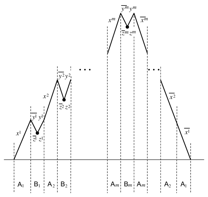
Figure 2: An instance of the form described in (3.2), as depicted in [MMN14, JN14]. A line segment with positive slope denotes a string over $\left\{a,b\right\}$, and a segment with negative slope denotes a string over $\left\{\overline{a},\overline{b}\right\}$. A solid dot depicts a pair of the form $\overline{z}z$ for some $z\in\left\{a,b\right\}$. The entire string is distributed amongst $2m$ players $\mathsf{A}_{1},\mathsf{B}_{1},\mathsf{A}_{2},\mathsf{B}_{2},\dotsc,\mathsf{A}_{m},\mathsf{B}_{m}$ in a communication protocol for ${\textsc{Ascension}}(m,n)$ as shown.

For ease of notation, the strings $x^{i}$ in ${\textsc{Ascension}}(m,n)$ are taken to be the ones in $\textsc{Dyck}(2)$ with the bits in reverse order. This converts the suffixes $y^{i}$ into prefixes of the same length.

As a consequence of the bijection above, any quantum streaming algorithm for Dyck(2) results in a quantum protocol for Ascension$(m,n)$, as stated in the following lemma.

Lemma 3.1

For any $\varepsilon\in[0,1/2]$, $n,m\in\mathbb{N}$, and for any $\varepsilon$-error (unidirectional) $T$-pass quantum streaming algorithm ${\mathcal{A}}$ for Dyck(2) that on instances of size $N\in\Theta(mn)$ uses $s(N)$ qubits of memory, there exists an $\varepsilon$-error, $T$-round sequential $(2m)$-party quantum communication protocol for Ascension$(m,n)$ in which each message is of length $s(N)$. The protocol may use public randomness, but does not use shared entanglement between any of the parties. Moreover, the local operations of the parties are memory-less, i.e., do not require access to the qubits used in generating the previous messages sent by that party.

Proof. Any random sequence of bits used by the streaming algorithm is provided as shared randomness to all the $2m$ parties in the communication protocol for Ascension$(m,n)$. Each input for the communication problem corresponds to an instance of Dyck(2), as described above. In each of the $T$ iterations, a player simulates the quantum streaming algorithm on appropriate part of the input for Dyck(2), and sends the length $s(N)$ workspace to the next player in the sequence. (If needed, non-unitary quantum operations may be replaced with an isometry, as follows from the Stinespring Representation theorem [Wat18].) The output of the protocol is the output of the algorithm, and is contained in the register held by the final party $\mathsf{A}_{1}$.   

3.2 Reduction from Augmented Index to Ascension

Recall that Ascension$(m,n)$ is composed of $m$ instances of Augmented Index on $n$ bits. Magniez, Mathieu, and Nayak [MMN14] showed how we may derive a low-information classical protocol for Augmented Index $f_{n}$ from one for Ascension$(m,n)$ through a direct sum argument (see Refs. [CCKM13, JN14] for the details of its working in the multi-pass case). This is not as straightforward to execute as it might first appear; it entails deriving a sequence of protocols for Augmented Index in which the communication from Alice to Bob corresponds to messages from different parties in the original multi-party protocol. We show that the same kind of construction, suitably adapted to the notion of quantum information cost we use, also works in the quantum case.

Let $\mu_{0}$ be the uniform distribution on the $0$-inputs of the Augmented Index function $f_{n}$. If $X$ is a uniformly random $n$-bit string, $K$ is a uniformly random index from $[n]$ independent of $X$, and the random variable $B$ is set as $B=X_{K}$, the joint distribution of $X,K,X[1,K-1],B$ is $\mu_{0}$. We denote the random variables $K,X[1,K-1],B$ given as input to Bob by $Y$. Since $X_{K}=B$ under this distribution, we abbreviate Bob’s input as $K,X[1,K]$. Let $\mu$ be the uniform distribution over all inputs. Under this distribution, the bit $B$ is uniformly random, independent of $XK$, while $XK$ are as above.

Lemma 3.2

Suppose $\varepsilon\in[0,1/2]$, $n,m\in\mathbb{N}$ and that there is an $\varepsilon$-error, $T$-round sequential quantum protocol $\Pi_{{\textsc{Asc}}}$ for Ascension$(m,n)$, that is memory-less, does not have shared entanglement between any of the parties (but might use public randomness), and only has messages of length at most $s$ (cf. Lemma 3.1). Then, there exists an $\varepsilon$-error, $2T$-message, two-party quantum protocol $\Pi_{{\textsc{AI}}}$ for the Augmented Index function $f_{n}$ that satisfies

$$\mathrm{QIC}_{{\mathrm{A}}\rightarrow{\mathrm{B}}}(\Pi_{\textsc{AI}},\mu_{0}) \quad\leq\quad 2sT\enspace,$$

$$\mathrm{QIC}_{{\mathrm{B}}\rightarrow{\mathrm{A}}}(\Pi_{\textsc{AI}},\mu_{0}) \quad\leq\quad 2sT/m\enspace.$$

Proof. Starting from the $(2m)$-party protocol $\Pi_{\textsc{Asc}}$ for Ascension$(m,n)$, we construct a protocol $\Pi_{j}$ for $f_{n}\,$, for each $j\in[m]$.

Fix one such $j$. Suppose Alice and Bob get inputs $x$ and $y$, respectively, where $y\coloneqq(k,x[1,k-1],b)$. They embed these into an instance of Ascension$(m,n)$: they set $x_{j}=x$, and $y_{j}=y$. They sample the inputs for the remaining $m-1$ coordinates independently, according to $\mu_{0}$. Let $X_{i}Y_{i}$, with $Y_{i}\coloneqq(K_{i},X_{i}[1,K_{i}])$, be registers corresponding to inputs drawn from $\mu_{0}$ in coordinate $i$. Let $R_{i}$ be a purification register for these, which we may decompose as $R_{i}^{X}R_{i}^{Y}$, denoting the standard purification of the $X_{i}Y_{i}$ registers. Let $S_{\mathrm{A}}S_{\mathrm{B}}$ be registers initialized to $\sum_{s}\sqrt{\nu_{s}}\mathop{\left|ss\right>}\nolimits$, so as to simulate the public random string $S\sim\nu$ used in the protocol $\Pi_{\textsc{Asc}}$.

For each $i\not=j$, we give $X_{i}$ to Alice, and $(K_{i},X_{i}[1,K_{i}])$ to Bob. For $i>j$, we give $R_{i}$ to Bob, and for $i<j$, we give $R_{i}$ to Alice. Then Alice and Bob simulate the roles of the $2m$ parties $(\mathsf{A}_{i},\mathsf{B}_{i})_{i\in[m]}$ in the following way for each of the $T$ rounds in $\Pi_{\textsc{Asc}}$. For $t=1,2,\dotsc,T$:

1. Alice simulates $\mathsf{A}_{1}\rightarrow\mathsf{B}_{1}\rightarrow\mathsf{A}_{2}\rightarrow\cdots\rightarrow\mathsf{A}_{j}$, accessing the inputs for $\mathsf{B}_{i}$, for $i<j$, in the register $R_{i}$. We denote the ancillary register she uses to implement $\mathsf{A}_{1}$’s local isometry via unitary operators by $D_{t1}$, and for all $i\in[2,j]$, the ancillary registers she uses for $\mathsf{B}_{i-1}$ and $\mathsf{A}_{i}$ together by $D_{ti}$.

2. Alice transmits the message from $\mathsf{A}_{j}$ to $\mathsf{B}_{j}$ to Bob.

3. Bob simulates $\mathsf{B}_{j}\rightarrow\mathsf{A}_{j+1}\rightarrow\cdots\rightarrow\mathsf{B}_{m}$, accessing the input for $\mathsf{A}_{i}$, for $i>j$, in the register $R_{i}$. For all $i$ such that $j\leq i<m$ we denote the ancillary registers Bob uses for implementing $\mathsf{B}_{i}$ and $\mathsf{A}_{i+1}$’s local isometry together by $D_{t(i+1)}$, and the ancillary register he uses for $\mathsf{B}_{m}$ by $D_{t(m+1)}$.

4. Bob transmits the message from $\mathsf{B}_{m}$ to $\mathsf{A}_{m}$ to Alice.

5. Alice simulates $\mathsf{A}_{m}\rightarrow\mathsf{A}_{m-1}\rightarrow\cdots\rightarrow\mathsf{A}_{1}$. We denote the ancillary registers Alice uses for implementing the local isometries of $\mathsf{A}_{m},\mathsf{A}_{m-1},\dotsc,\mathsf{A}_{2}$ together by $E_{t}$.

We let $E_{0}$ denote a dummy register initialized to a fixed state, say $\mathop{\left|0\right>}\nolimits$.

Since the inputs for Augmented Index for $i\neq j$ are distributed according to $\mu_{0}$, the protocol $\Pi_{j}$ computes Augmented Index for the instance $(x,y)$ with error at most $\varepsilon$.

The quantum information cost from Alice to Bob $\mathrm{QIC}_{{\mathrm{A}}\rightarrow{\mathrm{B}}}(\Pi_{j},\lambda)$ is bounded by $2sT$, for any distribution $\lambda$ over the inputs, as each of her $T$ messages has at most $s$ qubits.

The bound on quantum information cost from Bob to Alice arises from the following direct sum result. Suppose that the inputs for the protocol $\Pi_{j}$ for Augmented Index are drawn from the distribution $\mu_{0}$. Denote these inputs by $X_{j}Y_{j}$, with $Y_{j}\coloneqq(K_{j},X_{j}[1,K_{j}])$, and the corresponding purification register by $R_{j}$. We are interested in the quantum information cost $\mathrm{QIC}_{{\mathrm{B}}\rightarrow{\mathrm{A}}}(\Pi_{j},\mu_{0})$.

For $t\in[T]$, let $C_{t}$ denote the $t$th message from Bob to Alice in the protocol $\Pi_{j}$. At the time Alice receives message $C_{t}$, her other registers are $X_{1}\dotsb X_{m}$, $S_{\mathrm{A}}$, $R_{1}\dotsb R_{j-1}$, $(E_{r-1}D_{r1}D_{r2}\dotsb D_{rj})_{r\in[t]}$. Note that the corresponding state $\rho_{t}$ at that point on registers

$$X_{1}\dotsb X_{m}\;S_{\mathrm{A}}\;(E_{r-1}D_{r1}D_{r2}\dotsb D_{rm}D_{r(m+1)})_{r\in[t]}\;R_{1}\dotsb R_{m}\;C_{t}$$

is the same for all derived protocols $\Pi_{j}$, as all of them simulate $\Pi_{\textsc{Asc}}$ on the same input distribution, namely $\mu_{0}^{\otimes m}$, using the above registers.

We have

$$\mathrm{QIC}_{{\mathrm{B}}\rightarrow{\mathrm{A}}}(\Pi_{j},\mu_{0})$$

$$=\quad\sum_{t\in[T]}\operatorname{{\mathrm{I}}}(R_{j}\!:\!C_{t}\;|\;X_{1}\dotsb X_{m}S_{\mathrm{A}}(E_{r-1}D_{r1}D_{r2}\dotsb D_{rj})_{r\in[t]}R_{1}\dotsb R_{j-1})_{\rho_{t}}$$

$$\leq\quad\sum_{t\in[T]}\operatorname{{\mathrm{I}}}(R_{j}(D_{rj})_{r\in[t]}:C_{t}\;|\;X_{1}\dotsb X_{m}S_{\mathrm{A}}(E_{r-1}D_{r1}D_{r2}\dotsb D_{r(j-1)})_{r\in[t]}R_{1}\dotsb R_{j-1})_{\rho_{t}}\enspace.$$

Using the chain rule, we get

$$\sum_{j\in[m]}\mathrm{QIC}_{{\mathrm{B}}\rightarrow{\mathrm{A}}}(\Pi_{j},\mu_{0})$$

$$\leq\quad\sum_{t\in[T]}\operatorname{{\mathrm{I}}}(R_{1}\dotsb R_{m}(D_{r1}D_{r2}\dotsb D_{rm})_{r\in[t]}:C_{t}\;|\;X_{1}\dotsb X_{m}S_{\mathrm{A}}(E_{r-1})_{r\in[t]})_{\rho_{t}}\enspace.$$

Since each summand in the expression above is bounded by $2\log|C_{t}|$ and $\log|C_{t}|\leq s$, the sum is bounded by $2sT$. It follows that there exists an index $j^{*}$ such that

$$\mathrm{QIC}_{{\mathrm{B}}\rightarrow{\mathrm{A}}}(\Pi_{j^{*}},\mu_{0})\quad\leq\quad 2sT/m\enspace,$$

as desired. As noted before, $\mathrm{QIC}_{{\mathrm{A}}\rightarrow{\mathrm{B}}}(\Pi_{j^{*}},\mu_{0})\leq 2sT$. This completes the reduction.   

4 Key Technical Tools

In this section, we develop some tools needed to analyze the quantum information cost of protocols.

In analyzing safe quantum protocols with classical inputs in the rest of the paper, we deviate slightly from the notation for the registers used in the definition of two-party protocols in Section 2.1. We refer to the input registers $A_{\mathrm{in}},B_{\mathrm{in}}$ by $X,Y$, respectively. Since we focus on safe protocols, the registers $XY$ are only used as control registers. We express Alice’s local registers after the $i$th message is generated as $XA_{i}$, and the local registers of Bob by $YB_{i}$. As before, the message register is not included in any of the local registers, and is denoted by $C_{i}$.

4.1 Superposition-Average Encoding Theorem

We first generalize the Average Encoding Theorem [KNTZ07], to relate the quality of approximation of any intermediate state in a two-party quantum communication protocol to its information cost. This also allows us to analyze states arising from arbitrary superpositions over inputs in such protocols. Informally, the resulting statement is that if the incremental information contained in the messages received by a party is “small”, then she can approximate her part of the joint state “well”, without any assistance from the other party. The main technical ingredient of its proof is the Fawzi-Renner inequality [FR15].

Theorem 4.1 (Superposition-Average Encoding Theorem)

Given any safe quantum protocol $\Pi$ with input registers $XY$ initialized according to distribution $\nu$, let

$$\mathop{\left|\rho_{i}\right>}\nolimits\quad\coloneqq\quad\sum_{x,y}\sqrt{\nu(x,y)}\mathop{\left|xxyy\right>}\nolimits^{XR_{X}YR_{Y}}\mathop{\left|\rho_{i}^{xy}\right>}\nolimits^{A_{i}B_{i}C_{i}}$$

be the state of the registers $XYRA_{i}B_{i}C_{i}$ in round $i$ with the register $R$ initially purifying the registers $XY$, with a decomposition $R_{X}R_{Y}$ into coherent copies of $X$ and $Y$, respectively. Let $\varepsilon_{i}\coloneqq\operatorname{{\mathrm{I}}}(R\!:\!C_{i}\,|\,YB_{i})$ for odd $i$, and $\varepsilon_{i}\coloneqq\operatorname{{\mathrm{I}}}(R\!:\!C_{i}\,|\,XA_{i})$ for even $i$. There exist registers $E_{i}$, isometries $V_{i}$ and states $\mathop{\left|\theta_{i}\right>}\nolimits$ and $\mathop{\left|\theta^{y}_{i}\right>}\nolimits$ with

$$\mathop{\left|\theta_{i}\right>}\nolimits\quad=\quad\sum_{x,y}\sqrt{\nu(x,y)}\mathop{\left|xxyy\right>}\nolimits^{XR_{X}YR_{Y}}\mathop{\left|\theta_{i}^{y}\right>}\nolimits^{B_{i}C_{i}E_{i}}$$

for odd $i$ satisfying

$$\operatorname{{\mathfrak{h}}}\!\left(\rho_{i}^{RYB_{i}C_{i}},\theta_{i}^{RYB_{i}C_{i}}\right)\quad \leq\quad\sum_{p\leq i,~{}p~{}\mathrm{odd}}\sqrt{\varepsilon_{p}}\enspace,\qquad\textrm{and}$$ (4.1)

$$V_{i}\mathop{\left|y\right>}\nolimits^{Y}\quad =\quad\mathop{\left|y\right>}\nolimits^{Y}\otimes\mathop{\left|\theta_{i}^{y}\right>}\nolimits^{B_{i}C_{i}E_{i}}\enspace,$$

and states $\mathop{\left|\sigma_{i}\right>}\nolimits$ and $\mathop{\left|\sigma^{x}_{i}\right>}\nolimits$ with

$$\mathop{\left|\sigma_{i}\right>}\nolimits\quad=\quad\sum_{x,y}\sqrt{\nu(x,y)}\mathop{\left|xxyy\right>}\nolimits^{XR_{X}YR_{Y}}\mathop{\left|\sigma_{i}^{x}\right>}\nolimits^{A_{i}C_{i}E_{i}}$$

for even $i$ satisfying

$$\operatorname{{\mathfrak{h}}}\!\left(\rho_{i}^{RXA_{i}C_{i}},\sigma_{i}^{RXA_{i}C_{i}}\right)\quad \leq\quad\sum_{p\leq i,~{}p~{}\mathrm{even}}\sqrt{\varepsilon_{p}}\enspace,\qquad\textrm{and}$$ (4.2)

$$V_{i}\mathop{\left|x\right>}\nolimits^{X}\quad =\quad\mathop{\left|x\right>}\nolimits^{X}\otimes\mathop{\left|\sigma_{i}^{x}\right>}\nolimits^{A_{i}C_{i}E_{i}}\enspace.$$

Proof. The proofs for odd and even $i$’s are similar; we focus on even $i$’s. Given $\varepsilon_{p}\coloneqq\operatorname{{\mathrm{I}}}(R\!:\!C_{p}\,|\,XA_{p})$ for even $p$, let $\mathcal{R}_{p}^{XA_{p}\rightarrow XA_{p}C_{p}}$ be the recovery map given by the Fawzi-Renner inequality, Lemma 2.3, such that

$$\operatorname{{\mathfrak{h}}}\!\left(\rho_{p}^{RXA_{p}C_{p}},\mathcal{R}_{p}(\rho_{p}^{RXA_{p}})\right)\quad\leq\quad\sqrt{\varepsilon_{p}}\enspace,$$

and take $U_{\mathcal{R}_{p}}^{XA_{p}\rightarrow XA_{p}C_{p}F_{p}}$ to be an isometric extension of $\mathcal{R}_{p}$. Since register $R$ contains a coherent copy of $X$, we can assume without loss of generality that $U_{\mathcal{R}_{p}}^{XA_{p}\rightarrow XA_{p}C_{p}F_{p}}$ uses $X$ as a control register, i.e., acts as

$$U_{\mathcal{R}_{p}}^{XA_{p}\rightarrow XA_{p}C_{p}F_{p}}\mathop{\left|x\right>}\nolimits^{X}\mathop{\left|\phi\right>}\nolimits^{A_{p}G_{p}}\quad=\quad\mathop{\left|x\right>}\nolimits^{X}\mathop{\left|\phi_{x}\right>}\nolimits^{A_{p}C_{p}F_{p}G_{p}}\enspace,$$

for any state $\mathop{\left|\phi\right>}\nolimits$ of $A_{p}$ and ancillary register $G_{p}$, and any input $x$. Consider an isometry $V_{0}^{X\rightarrow XT_{\mathrm{A}}T_{\mathrm{B}}}$ such that for all $x$,

$$V_{0}\mathop{\left|x\right>}\nolimits^{X}\quad=\quad\mathop{\left|x\right>}\nolimits^{X}\mathop{\left|\psi\right>}\nolimits^{T_{\mathrm{A}}T_{\mathrm{B}}}\enspace,$$

i.e., $V_{0}$ is an isometry that locally creates the same state $\mathop{\left|\psi\right>}\nolimits^{T_{\mathrm{A}}T_{\mathrm{B}}}$, used as shared entanglement in $\Pi$, for any input $x$. Let $\rho_{\nu}$ denote the purified initial state of the protocol:

$$\mathop{\left|\rho_{\nu}\right>}\nolimits\quad\coloneqq\quad\sum_{x,y}\sqrt{\nu(x,y)}\mathop{\left|xxyy\right>}\nolimits^{XR_{X}YR_{Y}}\enspace.$$

We show that the isometry $V_{i}$, state $\sigma_{i}$, and register $E_{i}$ defined as follows

$$V_{i}\quad \coloneqq\quad U_{\mathcal{R}_{i}}U_{i-1}\cdots U_{\mathcal{R}_{4}}U_{3}U_{\mathcal{R}_{2}}U_{1}V_{0}\enspace,$$

$$\mathop{\left|\sigma_{i}\right>}\nolimits\quad \coloneqq\quad V_{i}\mathop{\left|\rho_{\nu}\right>}\nolimits\enspace,\qquad\textrm{and}$$

$$E_{i}\quad \coloneqq\quad T_{\mathrm{B}}\otimes C_{1}\otimes F_{2}\otimes C_{3}\otimes F_{4}\otimes\cdots\otimes C_{i-1}\otimes F_{i}$$

satisfy the conditions of the theorem. We show this by induction on $i$.

First, note that $V_{i}$ is of the desired form, and uses $X$ as a control register. For the base case, $i=2$, we start with

$$\mathop{\left|\rho_{0}\right>}\nolimits^{XYR_{X}R_{Y}T_{\mathrm{A}}T_{\mathrm{B}}}\quad=\quad V_{0}\mathop{\left|\rho_{\nu}\right>}\nolimits^{XYR_{X}R_{Y}}\enspace,$$

apply $U_{1}^{XT_{\mathrm{A}}\rightarrow XA_{1}C_{1}}$ to obtain $\mathop{\left|\rho_{1}\right>}\nolimits^{XYR_{X}R_{Y}A_{1}C_{1}T_{\mathrm{B}}}$, and furthermore apply $U_{2}^{YC_{1}T_{\mathrm{B}}\rightarrow YC_{2}B_{2}}$ to obtain $\mathop{\left|\rho_{2}\right>}\nolimits=U_{2}U_{1}V_{0}\mathop{\left|\rho_{\nu}\right>}\nolimits^{XYR_{X}R_{Y}}$. It holds that

$$\operatorname{{\mathfrak{h}}}\!\left(\rho_{2}^{RXA_{2}C_{2}},\mathcal{R}_{2}^{XA_{2}\rightarrow XA_{2}C_{2}}(\rho_{2}^{RXA_{2}})\right) \quad=\quad\operatorname{{\mathfrak{h}}}\!\left(\rho_{2}^{RXA_{2}C_{2}},\mathcal{R}_{2}^{XA_{1}\rightarrow XA_{2}C_{2}}(\rho_{1}^{RXA_{1}})\right)$$

$$\quad\leq\quad\sqrt{\varepsilon_{2}}\enspace,$$

in which we used that $\rho_{2}^{RXA_{2}}=\rho_{1}^{RXA_{1}}$ since the registers $YC_{2}B_{2}$ on which $U_{2}$ acts have been traced out, and $A_{2}=A_{1}$. Since it also holds that $\mathcal{R}_{2}(\rho_{1}^{RXA_{1}})=\mathop{{\mathrm{Tr}}_{YT_{\mathrm{B}}C_{1}F_{2}}}\left(U_{\mathcal{R}_{2}}U_{1}V_{0}\mathop{\left|\rho_{\nu}\right>}\nolimits\right)=\sigma_{2}^{RXA_{2}C_{2}}$, Eq. (4.2) follows.

For the induction step, we note that for even $i>2$, $V_{i}=U_{\mathcal{R}_{i}}U_{i-1}V_{i-2}$, $E_{i}=F_{i}\otimes C_{i-1}\otimes E_{i-2}$, and $\mathop{\left|\sigma_{i}\right>}\nolimits=U_{\mathcal{R}_{i}}U_{i-1}\mathop{\left|\sigma_{i-2}\right>}\nolimits$. Eq. (4.2) results from the following chain of inequalities, which are explained below:

$$\operatorname{{\mathfrak{h}}}\!\left(\rho_{i}^{RXA_{i}C_{i}},\sigma_{i}^{RXA_{i}C_{i}}\right)\quad\leq\quad \operatorname{{\mathfrak{h}}}\!\left(\rho_{i}^{RXA_{i}C_{i}},\mathcal{R}_{i}^{XA_{i}\rightarrow XA_{i}C_{i}}(\rho_{i}^{RXA_{i}})\right)$$

$$\mbox{}+\operatorname{{\mathfrak{h}}}\!\left(\mathcal{R}_{i}^{XA_{i}\rightarrow XA_{i}C_{i}}(\rho_{i}^{RXA_{i}}),\sigma_{i}^{RXA_{i}C_{i}}\right)$$

$$\quad\leq\quad \sqrt{\varepsilon_{i}}+\operatorname{{\mathfrak{h}}}\!\left(\rho_{i}^{RXA_{i}},\mathop{{\mathrm{Tr}}_{C_{i-1}YE_{i-2}}}\left(U_{i-1}\mathop{\left|\sigma_{i-2}\right>}\nolimits\right)\right)$$

$$\quad\leq\quad \sqrt{\varepsilon_{i}}+\operatorname{{\mathfrak{h}}}\!\left(\rho_{i-2}^{RXA_{i-2}C_{i-2}},\sigma_{i-2}^{RXA_{i-2}C_{i-2}}\right)$$

$$\quad\leq\quad \sqrt{\varepsilon_{i}}+\sum_{p\leq i-2,~{}p~{}\mathrm{even}}\sqrt{\varepsilon_{p}}\enspace.$$

The first step is an application of the triangle inequality, and the second follows by the definition of $\mathcal{R}_{i}$ and monotonicity of $h$ under the CPTP map $\mathcal{R}_{i}=\mathop{{\mathrm{Tr}}_{F_{i}}}\circ\,U_{\mathcal{R}_{i}}$. The third inequality holds because $\rho_{i}^{RXA_{i}}=\rho_{i-1}^{RXA_{i-1}}=\mathop{{\mathrm{Tr}}_{C_{i-1}YB_{i-2}}}\left(U_{i-1}\mathop{\left|\rho_{i-2}\right>}\nolimits\right)$, the isometry $U_{i-1}$ does not act on registers $E_{i-2}$ or $YB_{i-2}$, and by the monotonicity of $h$ under the map $\mathop{{\mathrm{Tr}}_{C_{i-1}}}\circ\,U_{i-1}$. The last inequality holds by the induction hypothesis. This completes the proof of the theorem.   

4.2 Quantum Cut-and-Paste Lemma

The direct quantum analogue to the Cut-and-Paste Lemma [BJKS04] from classical communication complexity does not hold. We can nevertheless obtain the following weaker property, linking the states in a two-party protocol corresponding to any four possible pairs of inputs in a two-by-two rectangle. The result implies that if the states corresponding to two inputs $x,x^{\prime}$ to Alice and a fixed input $y$ to Bob are close up to a local unitary operation on Alice’s side, and the states for two inputs $y,y^{\prime}$ to Bob and a fixed input $x$ to Alice are close up to a local unitary operation on Bob’s side, then, up to local unitary operations on Alice’s and Bob’s sides, the states for all pairs $(x^{\prime\prime},y^{\prime\prime})$ of inputs in the rectangle $\{x,x^{\prime}\}\times\{y,y^{\prime}\}$ are close. The lemma is a variant of the hybrid argument developed in Refs. [JRS03, JN14], and is proven along the same lines. A similar, albeit slightly weaker statement may be derived from the corresponding lemmas in these articles. For example, Lemma IV.10 from Ref. [JN14], when adapted to the setting described above and combined with a triangle inequality, implies bounds similar to those in Eqs. (4.4) and (4.6) below. However, in the notation of the lemma below, the bounds so derived are both larger by the additive term $2h_{i-1}$.

Lemma 4.2 (Quantum Cut-and-Paste)

Given any safe quantum protocol $\Pi$ with classical inputs, consider distinct inputs $x,x^{\prime}$ for Alice, and $y,y^{\prime}$ for Bob. Let $\mathop{\left|\rho_{0}\right>}\nolimits^{A_{0}B_{0}}$ be the shared initial state of Alice and Bob for any pair of inputs $(x^{\prime\prime},y^{\prime\prime})\in\{x,x^{\prime}\}\times\{y,y^{\prime}\}$. (The state $\rho_{0}$ may depend on the set $\{x,x^{\prime}\}\times\{y,y^{\prime}\}$.) Let $\mathop{\left|\rho_{i,x^{\prime\prime}y^{\prime\prime}}\right>}\nolimits^{A_{i}B_{i}C_{i}}$ be the state of registers $A_{i}B_{i}C_{i}$ after the $i$th message is sent, when the input is $(x^{\prime\prime},y^{\prime\prime})$. For odd $i$, let

$$h_{i}\quad\coloneqq\quad\operatorname{{\mathfrak{h}}}\!\left(\rho_{i,xy}^{B_{i}C_{i}},\rho_{i,x^{\prime}y}^{B_{i}C_{i}}\right)$$

and $V_{i,x\rightarrow x^{\prime}}^{A_{i}}$ denote the unitary operation acting on $A_{i}$ given by the Local Transition Lemma (Lemma 2.1) such that

$$h_{i}\quad=\quad\operatorname{{\mathfrak{h}}}\!\left(V_{i,x\rightarrow x^{\prime}}^{A_{i}}\mathop{\left|\rho_{i,xy}\right>}\nolimits\enspace,\mathop{\left|\rho_{i,x^{\prime}y}\right>}\nolimits\right)\enspace.$$

For even $i$, let

$$h_{i}\quad\coloneqq\quad\operatorname{{\mathfrak{h}}}\!\left(\rho_{i,xy}^{A_{i}C_{i}},\rho_{i,xy^{\prime}}^{A_{i}C_{i}}\right)$$

and $V_{i,y\rightarrow y^{\prime}}^{B_{i}}$ denote the unitary operation acting on $B_{i}$ given by the Local Transition Lemma such that

$$h_{i}\quad=\quad\operatorname{{\mathfrak{h}}}\!\left(V_{i,y\rightarrow y^{\prime}}^{B_{i}}\mathop{\left|\rho_{i,xy}\right>}\nolimits,\mathop{\left|\rho_{i,xy^{\prime}}\right>}\nolimits\right)\enspace.$$

Define $V_{0,y\rightarrow y^{\prime}}^{B_{0}}\coloneqq{\mathbb{I}}^{B_{0}}$ and $h_{0}\coloneqq 0$. Recall that $B_{i}=B_{i-1}$ for odd $i$ and $A_{i}=A_{i-1}$ for even $i$. It holds that for odd $i$,

$$\operatorname{{\mathfrak{h}}}\!\left(V_{i-1,y\rightarrow y^{\prime}}^{B_{i}}\mathop{\left|\rho_{i,xy}\right>}\nolimits,\mathop{\left|\rho_{i,xy^{\prime}}\right>}\nolimits\right) \quad=\quad h_{i-1}\enspace,$$ (4.3)

$$\operatorname{{\mathfrak{h}}}\!\left(V_{i,x\rightarrow x^{\prime}}^{A_{i}}V_{i-1,y\rightarrow y^{\prime}}^{B_{i}}\mathop{\left|\rho_{i,xy}\right>}\nolimits,\mathop{\left|\rho_{i,x^{\prime}y^{\prime}}\right>}\nolimits\right) \quad\leq\quad h_{i}+h_{i-1}+2\sum_{j=1}^{i-2}h_{j}\enspace,$$ (4.4)

and for even $i$,

$$\operatorname{{\mathfrak{h}}}\!\left(V_{i-1,x\rightarrow x^{\prime}}^{A_{i}}\mathop{\left|\rho_{i,xy}\right>}\nolimits,\mathop{\left|\rho_{i,x^{\prime}y}\right>}\nolimits\right) \quad=\quad h_{i-1}\enspace,$$ (4.5)

$$\operatorname{{\mathfrak{h}}}\!\left(V_{i,y\rightarrow y^{\prime}}^{B_{i}}V_{i-1,x\rightarrow x^{\prime}}^{A_{i}}\mathop{\left|\rho_{i,xy}\right>}\nolimits,\mathop{\left|\rho_{i,x^{\prime}y^{\prime}}\right>}\nolimits\right) \quad\leq\quad h_{i}+h_{i-1}+2\sum_{j=1}^{i-2}h_{j}\enspace.$$ (4.6)

Proof. We have $\mathop{\left|\rho_{0,x^{\prime\prime}y^{\prime\prime}}\right>}\nolimits=\mathop{\left|\rho_{0}\right>}\nolimits$, and define $C_{0}$ to be a trivial register. For odd $i$, let $U_{i,x^{\prime\prime}}$ be the protocol isometry $U_{i}$ conditional on the state of $X$ being $\mathop{\left|x^{\prime\prime}\right>}\nolimits$. Then we have

$$U_{i,x^{\prime\prime}}^{A_{i-1}C_{i-1}\rightarrow A_{i}C_{i}}\mathop{\left|\rho_{i-1,x^{\prime\prime}y^{\prime\prime}}\right>}\nolimits^{A_{i-1}B_{i-1}C_{i-1}}\quad=\quad\mathop{\left|\rho_{i,x^{\prime\prime}y^{\prime\prime}}\right>}\nolimits^{A_{i}B_{i}C_{i}}\enspace.$$

It follows by the isometric invariance of $h$ and because $V_{i-1,y\rightarrow y^{\prime}}$ and $U_{i,x}$ act on disjoint sets of registers that

$$\operatorname{{\mathfrak{h}}}\!\left(V_{i-1,y\rightarrow y^{\prime}}^{B_{i}}\mathop{\left|\rho_{i,xy}\right>}\nolimits,\mathop{\left|\rho_{i,xy^{\prime}}\right>}\nolimits\right) \quad=\quad\operatorname{{\mathfrak{h}}}\!\left(V_{i-1,y\rightarrow y^{\prime}}^{B_{i-1}}\mathop{\left|\rho_{i-1,xy}\right>}\nolimits,\mathop{\left|\rho_{i-1,xy^{\prime}}\right>}\nolimits\right)$$

$$\quad=\quad h_{i-1}\enspace.$$

Similarly, for even $i$,

$$U_{i,y^{\prime\prime}}^{B_{i-1}C_{i-1}\rightarrow B_{i}C_{i}}\mathop{\left|\rho_{i-1,x^{\prime\prime}y^{\prime\prime}}\right>}\nolimits^{A_{i-1}B_{i-1}C_{i-1}}\quad=\quad\mathop{\left|\rho_{i,x^{\prime\prime}y^{\prime\prime}}\right>}\nolimits^{A_{i}B_{i}C_{i}}$$

and

$$\operatorname{{\mathfrak{h}}}\!\left(V_{i-1,x\rightarrow x^{\prime}}^{A_{i}}\mathop{\left|\rho_{i,xy}\right>}\nolimits,\mathop{\left|\rho_{i,x^{\prime}y}\right>}\nolimits\right) \quad=\quad h_{i-1}\enspace.$$

This proves Eqs. (4.3) and (4.5).

We show by induction on $i$ that Eqs. (4.4) and (4.6) hold for odd and even $i$’s, respectively. For the base case ($i=1$), we have that

$$\mathop{\left|\rho_{1,x^{\prime\prime}y^{\prime\prime}}\right>}\nolimits^{A_{1}B_{1}C_{1}}\quad=\quad U_{x^{\prime\prime}}^{A_{0}\rightarrow A_{1}C_{1}}\mathop{\left|\rho_{0}\right>}\nolimits^{A_{0}B_{0}}\enspace,$$

and is independent of $y^{\prime\prime}$. So

$$\mathop{\left|\rho_{1,xy}\right>}\nolimits\quad=\quad\mathop{\left|\rho_{1,xy^{\prime}}\right>}\nolimits\enspace,\qquad\mathrm{and}\qquad\mathop{\left|\rho_{1,x^{\prime}y}\right>}\nolimits\quad=\quad\mathop{\left|\rho_{1,x^{\prime}y^{\prime}}\right>}\nolimits\enspace,$$

and Eq. (4.4) follows by taking $V_{0,y\rightarrow y^{\prime}}^{B_{0}}\coloneqq{\mathbb{I}}^{B_{0}}$:

$$\operatorname{{\mathfrak{h}}}\!\left(V_{1,x\rightarrow x^{\prime}}^{A_{1}}\mathop{\left|\rho_{1,xy}\right>}\nolimits,\mathop{\left|\rho_{1,x^{\prime}y^{\prime}}\right>}\nolimits\right) \quad=\quad h_{1}\enspace.$$

For the induction step (with $i\geq 2$), the case of even and odd $i$’s are proven similarly; we focus on even $i$’s. Assuming that Eq. (4.4) holds for $i-1$, we show Eq. (4.6) holds for $i$ by the following chain of inequalities which are explained below:

$$\operatorname{{\mathfrak{h}}}\!\left(V_{i,y\rightarrow y^{\prime}}^{B_{i}}V_{i-1,x\rightarrow x^{\prime}}^{A_{i}}\mathop{\left|\rho_{i,xy}\right>}\nolimits,\mathop{\left|\rho_{i,x^{\prime}y^{\prime}}\right>}\nolimits\right)\quad\leq\quad \operatorname{{\mathfrak{h}}}\!\left(V_{i,y\rightarrow y^{\prime}}^{B_{i}}V_{i-1,x\rightarrow x^{\prime}}^{A_{i}}\mathop{\left|\rho_{i,xy}\right>}\nolimits,V_{i-1,x\rightarrow x^{\prime}}^{A_{i}}\mathop{\left|\rho_{i,xy^{\prime}}\right>}\nolimits\right)$$

$$+\operatorname{{\mathfrak{h}}}\!\left(V_{i-1,x\rightarrow x^{\prime}}^{A_{i}}\mathop{\left|\rho_{i,xy^{\prime}}\right>}\nolimits,\mathop{\left|\rho_{i,x^{\prime}y^{\prime}}\right>}\nolimits\right)$$

$$\quad=\quad h_{i}+\operatorname{{\mathfrak{h}}}\!\left(V_{i-1,x\rightarrow x^{\prime}}^{A_{i-1}}\mathop{\left|\rho_{i-1,xy^{\prime}}\right>}\nolimits,\mathop{\left|\rho_{i-1,x^{\prime}y^{\prime}}\right>}\nolimits\right)$$

$$\quad\leq\quad h_{i}+\operatorname{{\mathfrak{h}}}\!\left(V_{i-1,x\rightarrow x^{\prime}}^{A_{i-1}}\mathop{\left|\rho_{i-1,xy^{\prime}}\right>}\nolimits,V_{i-1,x\rightarrow x^{\prime}}^{A_{i-1}}V_{i-2,y\rightarrow y^{\prime}}^{B_{i-1}}\mathop{\left|\rho_{i-1,xy}\right>}\nolimits\right)$$

$$+\operatorname{{\mathfrak{h}}}\!\left(V_{i-1,x\rightarrow x^{\prime}}^{A_{i-1}}V_{i-2,y\rightarrow y^{\prime}}^{B_{i-1}}\mathop{\left|\rho_{i-1,xy}\right>}\nolimits,\mathop{\left|\rho_{i-1,x^{\prime}y^{\prime}}\right>}\nolimits\right)$$

$$\quad\leq\quad h_{i}+h_{i-2}+h_{i-1}+h_{i-2}+2\sum_{j=1}^{i-3}h_{j}\enspace.$$

The first step is by the triangle inequality. In the second step, we used the unitary invariance of $\operatorname{{\mathfrak{h}}}$ along with the definition of $h_{i}$ for the first term, and with the property that $V_{i-1}^{A_{i}}$ and $U_{i,y^{\prime}}^{B_{i-1}C_{i-1}\rightarrow B_{i}C_{i}}$ act on disjoint sets of registers for the second term. The next step follows by the triangle inequality. The last step is by Eq. (4.3) for the second term, and by the induction hypothesis (Eq. (4.4)) for the third term.   

5 QIC Lower Bound for Augmented Index

In this section, we establish a lower bound for the quantum information cost of protocols for Augmented Index.

5.1 Relating Alice’s states to $\mathrm{QIC}_{{\mathrm{B}}\rightarrow A}$

We study the quantum information cost of protocols for Augmented Index on input distribution $\mu_{0}$ (the uniform distribution over $f_{n}^{-1}(0)$), and relate it to the distance between the states on two different inputs. We first focus on the quantum information cost from Bob to Alice, arising from the messages with even $i$’s. We show that if this cost is low, then Alice’s reduced states on different inputs for Bob are close to each other. (This high level intuition is the same as that described in Ref. [JN14].)

We state and prove our results for inputs with even length $n$; a similar result can be shown for odd $n$ by suitably adapting the proof.

We consider the following purification of the input registers, corresponding to a particular preparation method for the $K$ register, and to a preparation of the $X$ register also depending on the preparation of register $K$. Recall that the content $k$ of register $K$ is uniformly distributed in $[n]$. The following registers are each initialized to uniform superpositions over the domain indicated: $R_{S}^{1}$ over $\left\{0,1\right\}$ (with a coherent copy in $R_{S}^{2}$), register $R_{J}^{1}$ over indices $j\in[n/2]$ (with a coherent copy in $R_{J}^{2}$), register $R_{L}^{1}$ over $\ell\in[n/2+1,n]$ (with a coherent copy in $R_{L}^{2}$). Register $R_{K}$ holds a coherent copy of register $K$, whose content $k$ is set to the value $j$ in $R_{J}^{1}$ when $R_{S}^{1}$ is $0$, and to $\ell$ when $R_{S}^{1}$ is $1$. Depending on the value $\ell$ of $R_{L}^{1}$, the following registers are initialized to uniform superpositions to prepare the $X$ register, itself uniform over $\{0,1\}^{n}$: register $R_{Z}^{1}$ over $z\in\{0,1\}^{\ell}$, and register $R_{W}^{1}$ over $w\in\{0,1\}^{n-\ell}$. The register $X$ is set to $x=zw$, so together $R_{Z}^{1}R_{W}^{1}$ hold a coherent copy of $X$, and a second coherent copy is held in $R_{Z}^{2}R_{W}^{2}$. If $\ell$ is clear from the context, we sometimes use the notation $Z$ and $W$ to refer to the parts of the $X$ register holding $z$ and $w$, respectively. Depending on the value $j$ of $R_{J}^{1}$, we also refer to a further decomposition $z=z^{\prime}z^{\prime\prime}$ with $z^{\prime}\in\{0,1\}^{j}$ and $z^{\prime\prime}\in\{0,1\}^{\ell-j}$. We denote by $X_{1K}$ the register held by Bob, containing the first $k-1$ bits of $x$ and the verification bit $b$. The bit $b$ is always equal to $x_{k}$ under $\mu_{0}$; $X_{1K}$ thus contains the first $k$ bits of $x$ in this case. The register $X_{1K}$ is set to $z^{\prime}$ when $R_{S}^{1}$ is $0$, to $z$ when $R_{S}^{1}$ is 1, and register $R_{X_{1K}}$ holds a coherent copy of $X_{1K}$.

In summary, the resulting input state $\rho_{\mu_{0}}^{XKX_{1K}}$ distributed according to $\mu_{0}$ is purified by register $R$, which decomposes as

$$R\quad\coloneqq\quad R_{J}^{1}R_{J}^{2}R_{L}^{1}R_{L}^{2}R_{Z}^{1}R_{Z}^{2}R_{W}^{1}R_{W}^{2}R_{S}^{1}R_{S}^{2}R_{K}R_{X_{1K}}\enspace.$$

Using the normalization factor $c\coloneqq 1/\sqrt{(n/2)\cdot(n/2)\cdot 2^{\ell}\cdot 2^{n-\ell}\cdot 2}$, the purified state is:

$$\mathop{\left|\rho_{0}\right>}\nolimits^{RXKX_{1K}}\quad\coloneqq\quad c\sum_{j,\ell,z,w}\mathop{\left|jj\ell\ell zzww\right>}\nolimits\left(\mathop{\left|00\right>}\nolimits\mathop{\left|jz^{\prime}\right>}\nolimits\mathop{\left|zw\right>}\nolimits^{X}\mathop{\left|jz^{\prime}\right>}\nolimits^{KX_{1K}}+\mathop{\left|11\right>}\nolimits\mathop{\left|\ell z\right>}\nolimits\mathop{\left|zw\right>}\nolimits^{X}\mathop{\left|\ell z\right>}\nolimits^{KX_{1K}}\right)\enspace.$$ (5.1)

Starting with the above purification and using shared entanglement $\mathop{\left|\psi\right>}\nolimits^{T_{\mathrm{A}}T_{\mathrm{B}}}$ in the initial state, the state $\rho_{i}$ over the registers $RXKX_{1K}A_{i}B_{i}C_{i}$ after round $i$ in the protocol is

$$\mathop{\left|\rho_{i}\right>}\nolimits\quad\coloneqq\quad c\sum_{j,\ell,z,w}\mathop{\left|jj\ell\ell zzww\right>}\nolimits\left(\mathop{\left|00\right>}\nolimits\mathop{\left|jz^{\prime}\right>}\nolimits\mathop{\left|zw\right>}\nolimits\mathop{\left|jz^{\prime}\right>}\nolimits\mathop{\left|\rho_{i}^{zw,(j,z^{\prime})}\right>}\nolimits+\mathop{\left|11\right>}\nolimits\mathop{\left|\ell z\right>}\nolimits\mathop{\left|zw\right>}\nolimits\mathop{\left|\ell z\right>}\nolimits\mathop{\left|\rho_{i}^{zw,(\ell,z)}\right>}\nolimits\right)\enspace,$$ (5.2)

where $\mathop{\left|\rho_{i}^{x,(k,x[1,k])}\right>}\nolimits$ denotes the pure state in registers $A_{i}B_{i}C_{i}$ conditional on joint input $\left(x,(k,x[1,k])\right)$.

Define $R_{\mathrm{A}}\coloneqq R_{J}^{1}R_{L}^{1}R_{S}^{1}R_{K}R_{W}^{1}R_{W}^{2}$. All of $R_{\mathrm{A}}$’s sub-registers except $R_{W}^{1}R_{W}^{2}$ are classical in $\rho_{i}^{R_{A}XA_{i}C_{i}}$, since one of their coherent copies is traced out from the global purification register $R$. The $Z$ part of the $X$ register is also classical. We can write the reduced state of $\rho_{i}$ on registers $R_{A}XA_{i}C_{i}$ as

$$\rho_{i}^{R_{A}XA_{i}C_{i}}\quad=\quad c^{\prime}\sum_{j,\ell,z}\left|j\ell\right\rangle\!\left\langle j\ell\right|\otimes\left(\left|0j\right\rangle\!\left\langle 0j\right|\otimes\left|z\right\rangle\!\left\langle z\right|^{Z}\otimes\rho_{i,\ell zjz^{\prime}}+\left|1\ell\right\rangle\!\left\langle 1\ell\right|\otimes\left|z\right\rangle\!\left\langle z\right|^{Z}\otimes\rho_{i,\ell z\ell z}\right)\enspace,$$

in which we used normalization $c^{\prime}\coloneqq 1/((n/2)\cdot(n/2)\cdot 2^{\ell}\cdot 2)$ and the shorthands

$$\rho_{i,\ell zkx[1,k]}\quad\coloneqq\quad \mathop{{\mathrm{Tr}}_{B_{i}}}\left(\left|\rho_{i}^{\ell zkx[1,k]}\right\rangle\!\left\langle\rho_{i}^{\ell zkx[1,k]}\right|\right)\enspace,\qquad\textrm{where}$$ (5.3)

$$\mathop{\left|\rho_{i}^{\ell zkx[1,k]}\right>}\nolimits\quad\coloneqq\quad 1/\sqrt{2^{n-\ell}}\sum_{w}\mathop{\left|www\right>}\nolimits^{R_{W}^{1}R_{W}^{2}W}\mathop{\left|\rho_{i}^{zw,(k,x[1,k])}\right>}\nolimits^{A_{i}B_{i}C_{i}}\enspace.$$ (5.4)

The indices $\ell zkx[1,k]$ have the following meaning: $\ell$ and $z$ indicate that Alice’s input register $X$ is in superposition after the length $\ell$ prefix $z$ (with $z=x[1,\ell]$); $k$ and $x[1,k]$ tell us the index $k$ in Bob’s input, the prefix $x[1,k-1]$ of $x$ given as input to Bob, and Bob’s verification bit $b$ (which is equal to $x_{k}$ under $\mu_{0}$), respectively. Using this notation along with the superposition-average encoding theorem, we show the following result.

Lemma 5.1

Given any even $n\geq 2$, let $J$ and $L$ be random variables uniformly distributed in $[n/2]$ and $[n]\setminus[n/2]$, respectively. Conditional on some value $\ell$ for $L$, let $Z$ be a random variable chosen uniformly at random in $\{0,1\}^{\ell}$. The following then holds for any $M$-message safe quantum protocol $\Pi$ for Augmented Index $f_{n}\,$, for any even $i\leq M$:

$$\mathrm{QIC}_{{\mathrm{B}}\rightarrow A}(\Pi,\mu_{0})\quad\geq\quad\frac{1}{2M}\;\mathbb{E}_{j\ell z\sim JLZ}\left[\operatorname{{\mathfrak{h}}}^{2}\!\left(\rho_{i,\ell zjz^{\prime}}^{R_{W}^{1}R_{W}^{2}WA_{i}C_{i}},\rho_{i,\ell z\ell z}^{R_{W}^{1}R_{W}^{2}WA_{i}C_{i}}\right)\right]\enspace.$$

Proof. Considering the same purification of the input state as in Eq. (5.1), we get the following states from the superposition-average encoding theorem

$$\mathop{\left|\sigma_{i}\right>}\nolimits\quad\coloneqq\quad c\sum_{j,\ell,z,w}\mathop{\left|jj\ell\ell zzww\right>}\nolimits\left(\mathop{\left|00\right>}\nolimits\mathop{\left|jz^{\prime}\right>}\nolimits\mathop{\left|zw\right>}\nolimits\mathop{\left|jz^{\prime}\right>}\nolimits\mathop{\left|\sigma_{i}^{zw}\right>}\nolimits^{A_{i}C_{i}E_{i}}+\mathop{\left|11\right>}\nolimits\mathop{\left|\ell z\right>}\nolimits\mathop{\left|zw\right>}\nolimits\mathop{\left|\ell z\right>}\nolimits\mathop{\left|\sigma_{i}^{zw}\right>}\nolimits^{A_{i}C_{i}E_{i}}\right)\enspace,$$

satisfying

$$\operatorname{{\mathfrak{h}}}(\rho_{i}^{RXA_{i}C_{i}},\sigma_{i}^{RXA_{i}C_{i}})\quad\leq\quad \sum_{p\leq i,~{}p~{}\mathrm{even}}\sqrt{\operatorname{{\mathrm{I}}}(C_{p}\!:\!R\,|\,XA_{p})}\enspace.$$

The reduced state of $\sigma_{i}$ on registers $R_{\mathrm{A}}XA_{i}C_{i}$ is

$$\sigma_{i}^{R_{\mathrm{A}}XA_{i}C_{i}}\quad=\quad c^{\prime}\sum_{j,\ell,z}\left|j\ell\right\rangle\!\left\langle j\ell\right|\otimes\left(\left|0j\right\rangle\!\left\langle 0j\right|\otimes\left|z\right\rangle\!\left\langle z\right|^{Z}\otimes\sigma_{i,\ell z}+\left|1\ell\right\rangle\!\left\langle 1\ell\right|\otimes\left|z\right\rangle\!\left\langle z\right|^{Z}\otimes\sigma_{i,\ell z}\right)\enspace,$$

in which we use the shorthands

$$\sigma_{i,\ell z}\quad\coloneqq\quad \mathop{{\mathrm{Tr}}_{E_{i}}}\left(\left|\sigma_{i}^{\ell z}\right\rangle\!\left\langle\sigma_{i}^{\ell z}\right|\right)\enspace,\quad\textrm{where}$$

$$\mathop{\left|\sigma_{i}^{\ell z}\right>}\nolimits\quad\coloneqq\quad \frac{1}{\sqrt{2^{n-\ell}}}\;\sum_{w}\mathop{\left|www\right>}\nolimits^{R_{W}^{1}R_{W}^{2}W}\mathop{\left|\sigma_{i}^{zw}\right>}\nolimits^{A_{i}C_{i}E_{i}}\enspace.$$

The lemma then follows from the next chain of inequalities, as explained below:

$$\frac{i}{2}\sum_{p\leq i,~{}p~{}\mathrm{even}}\operatorname{{\mathrm{I}}}(C_{p}\!:\!R\,|\,XA_{p})\quad\geq\quad \left(\sum_{p\leq i,~{}p~{}\mathrm{even}}\sqrt{\operatorname{{\mathrm{I}}}(C_{p}\!:\!R\,|\,XA_{p})}\right)^{2}$$

$$\quad\geq\quad \operatorname{{\mathfrak{h}}}^{2}\!\left(\rho_{i}^{R_{\mathrm{A}}ZWA_{i}C_{i}},\sigma_{i}^{R_{\mathrm{A}}ZWA_{i}C_{i}}\right)$$

$$\quad=\quad \frac{1}{2}\;\mathbb{E}_{j\ell z\sim JLZ}\left[\operatorname{{\mathfrak{h}}}^{2}\!\left(\rho_{i,\ell zjz^{\prime}}^{R_{W}^{1}R_{W}^{2}WA_{i}C_{i}},\sigma_{i,\ell z}^{R_{W}^{1}R_{W}^{2}WA_{i}C_{i}}\right)\right]$$

$$+\frac{1}{2}\;\mathbb{E}_{j\ell z\sim JLZ}\left[\operatorname{{\mathfrak{h}}}^{2}\!\left(\rho_{i,\ell z\ell z}^{R_{W}^{1}R_{W}^{2}WA_{i}C_{i}},\sigma_{i,\ell z}^{R_{W}^{1}R_{W}^{2}WA_{i}C_{i}}\right)\right]$$

$$\quad\geq\quad \frac{1}{4}\;\mathbb{E}_{j\ell z\sim JLZ}\left[\operatorname{{\mathfrak{h}}}^{2}\!\left(\rho_{i,\ell zjz^{\prime}}^{R_{W}^{1}R_{W}^{2}WA_{i}C_{i}},\rho_{i,\ell z\ell z}^{R_{W}^{1}R_{W}^{2}WA_{i}C_{i}}\right)\right]\enspace.$$

The first inequality is by the concavity of the square root function and the Jensen inequality, and the second by the superposition-average encoding theorem along with the monotonicity of $\operatorname{{\mathfrak{h}}}$ under tracing out a part of register $R$. The equality is by the joint linearity of $\operatorname{{\mathfrak{h}}}^{2}$ (cf. Eq. (2.3)), by expanding the expectation over $R_{S}^{1}$ and by fixing $k$ accordingly. The last inequality is by the weak triangle inequality of $\operatorname{{\mathfrak{h}}}^{2}$ (cf. Eq. (2.4)).   

5.2 Relating Bob’s states to $\mathrm{QIC}_{{\mathrm{A}}\rightarrow{\mathrm{B}}}$

We continue with the notation from the previous section, and now focus on the quantum information cost from Alice to Bob, arising from messages with odd $i$’s. We go via an alternative notion of information cost used by Jain and Nayak [JN14], and studied further by Laurière and Touchette [LT17a, LT17b]. This notion is similar to the internal information cost of classical protocols (see, e.g., Refs. [BJKS04, BBCR13]), and is called the Holevo information cost in Ref. [LT17b].

Definition 5.2

Given a safe quantum protocol $\Pi$ with classical inputs, and distribution $\nu$ over inputs, the Holevo information cost (of the messages) from Alice to Bob in round $i$ is defined as

$$\widetilde{\mathrm{QIC}}_{{\mathrm{A}}\rightarrow{\mathrm{B}}}^{i}(\Pi,\nu)\quad=\quad \operatorname{{\mathrm{I}}}(X\!:\!B_{i}C_{i}\,|\,Y)\enspace,$$

and the cumulative Holevo information cost from Alice to Bob is defined as

$$\widetilde{\mathrm{QIC}}_{{\mathrm{A}}\rightarrow{\mathrm{B}}}(\Pi,\nu)\quad=\quad \sum_{i~{}\mathrm{odd}}\widetilde{\mathrm{QIC}}_{{\mathrm{A}}\rightarrow{\mathrm{B}}}^{i}(\Pi,\nu)\enspace.$$

Given a bit string $z$ of length at least $\ell\geq 1$, let $z^{(\ell)}$ denote the string obtained by flipping the $\ell$th bit of $z$. The following result can be inferred from the proof of Lemma 4.9 in Ref. [JN14].

Lemma 5.3

Given any even $n\geq 2$, let $J$ and $L$ be random variables uniformly distributed in $[n/2]$ and $[n]\setminus[n/2]$, respectively. Conditional on some value $\ell$ for $L$, let $Z$ be a random variable chosen uniformly at random in $\{0,1\}^{\ell}$. The following holds for any $M$-message safe quantum protocol $\Pi$ for the Augmented Index function $f_{n}\,$, for any odd $i\leq M$:

$$\frac{1}{n}\;\widetilde{\mathrm{QIC}}_{{\mathrm{A}}\rightarrow{\mathrm{B}}}^{i}(\Pi,\mu_{0})\quad\geq\quad\frac{1}{16}\;\mathbb{E}_{j\ell z\sim JLZ}\left[\operatorname{{\mathfrak{h}}}^{2}\!\left(\rho_{i,\ell zjz^{\prime}}^{B_{i}C_{i}}~{},~{}\rho_{i,\ell z^{(\ell)}jz^{\prime}}^{B_{i}C_{i}}\right)\right]\enspace,$$

with $\rho_{i,\ell zjz^{\prime}}$ defined by Eqs. (5.3) and (5.4).

For completeness, we provide a proof of this lemma in Appendix A using our notation.

Laurière and Touchette [LT17a, LT17b] prove that Holevo information cost is a lower bound on quantum information cost.

Lemma 5.4

Given any $M$-message quantum protocol $\Pi$ and any input distribution $\nu$, the following holds for any odd $i\leq M$:

$$\widetilde{\mathrm{QIC}}_{{\mathrm{A}}\rightarrow{\mathrm{B}}}^{i}(\Pi,\nu)\quad\leq\quad\mathrm{QIC}_{{\mathrm{A}}\rightarrow{\mathrm{B}}}(\Pi,\nu)\enspace.$$

This may be derived from the Information Flow Lemma (Lemma 2.6) by initializing the purification register $R$ so that $R_{a}^{\mathrm{B}}$ is a coherent copy of $X$ and $R_{b}^{\mathrm{B}}$ is a coherent copy of $Y$, and $R_{c}^{\mathrm{B}}$ is a coherent copy of both $X,Y$.

5.3 Lower bound on QIC

We are now ready to prove a slightly weaker variant of our main lower bound (Theorem 6.1) on the quantum information cost of Augmented Index.

Theorem 5.5

Given any even $n$, the following holds for any $M$-message safe quantum protocol $\Pi$ computing the Augmented Index function $f_{n}$ with error at most $\varepsilon$ on any input:

$$\frac{1}{4}(1-2\varepsilon)\quad\leq\quad \left(\frac{2(M+1)^{2}}{n}\cdot\mathrm{QIC}_{{\mathrm{A}}\rightarrow{\mathrm{B}}}(\Pi,\mu_{0})\right)^{1/2}+\left(\frac{M^{3}}{4}\cdot\mathrm{QIC}_{{\mathrm{B}}\rightarrow{\mathrm{A}}}(\Pi,\mu_{0})\right)^{1/2}\enspace.$$

The stronger version is proven similarly in Section 6 using a strengthening of Lemma 5.1. Our argument follows ideas similar to those in Ref. [JN14]. Using the notation from the two previous sections, we start by fixing values of $j,\ell,z$ in their respective domains, and defining $\hat{A}_{i}\coloneqq R_{W}^{1}R_{W}^{2}WA_{i}$. Define, for odd $i$,

$$h_{i}(j,\ell,z) \quad\coloneqq\quad\operatorname{{\mathfrak{h}}}\!\left(\rho_{i,\ell zjz^{\prime}}^{B_{i}C_{i}}~{},~{}\rho_{i,\ell z^{(\ell)}jz^{\prime}}^{B_{i}C_{i}}\right)$$

$$\quad=\quad\operatorname{{\mathfrak{h}}}\!\left(V_{i,z\rightarrow z^{(\ell)}}^{\hat{A}_{i}}\mathop{\left|\rho_{i}^{\ell zjz^{\prime}}\right>}\nolimits^{\hat{A}_{i}B_{i}C_{i}}\enspace,\mathop{\left|\rho_{i}^{\ell z^{(\ell)}jz^{\prime}}\right>}\nolimits^{\hat{A}_{i}B_{i}C_{i}}\right)\enspace,$$

and for even $i$,

$$h_{i}(j,\ell,z) \quad\coloneqq\quad\operatorname{{\mathfrak{h}}}\!\left(\rho_{i,\ell zjz^{\prime}}^{\hat{A}_{i}C_{i}},\rho_{i,\ell z\ell z}^{\hat{A}_{i}C_{i}}\right)$$

$$\quad=\quad\operatorname{{\mathfrak{h}}}\!\left(V_{i,(j,z^{\prime})\rightarrow(\ell,z)}^{B_{i}}\mathop{\left|\rho_{i}^{\ell zjz^{\prime}}\right>}\nolimits^{\hat{A}_{i}B_{i}C_{i}}\enspace,\mathop{\left|\rho_{i}^{\ell z\ell z}\right>}\nolimits^{\hat{A}_{i}B_{i}C_{i}}\right)\enspace,$$

where the unitary operations $V_{i,z\rightarrow z^{(\ell)}}^{\hat{A}_{i}}$ and $V_{i,(j,z^{\prime})\rightarrow(\ell,z)}^{B_{i}}$ are given by the Local Transition Lemma. We define the following states, analogous to the states consistent with $\mu_{0}$ in Eqs. (5.3) and (5.4):

$$\rho_{i,\ell z^{(\ell)}\ell z}\quad\coloneqq\quad \mathop{{\mathrm{Tr}}_{B_{i}}}\left(\left|\rho_{i}^{\ell z^{(\ell)}\ell z}\right\rangle\!\left\langle\rho_{i}^{\ell z^{(\ell)}\ell z}\right|\right)\enspace,$$

$$\mathop{\left|\rho_{i}^{\ell z^{(\ell)}\ell z}\right>}\nolimits\quad\coloneqq\quad \frac{1}{\sqrt{2^{n-\ell}}}\sum_{w}\mathop{\left|www\right>}\nolimits^{R_{W}^{1}R_{W}^{2}W}\mathop{\left|\rho_{i}^{z^{(\ell)}w,(\ell,z)}\right>}\nolimits^{A_{i}B_{i}C_{i}}\enspace.$$

Given protocol $\Pi$, we define a protocol $\Pi(j,\ell,z)$ that behaves as $\Pi$ but starts with shared entanglement $\mathop{\left|\psi\right>}\nolimits^{T_{\mathrm{A}}T_{\mathrm{B}}}\otimes\mathop{\left|\psi_{W}\right>}\nolimits$, with $\mathop{\left|\psi_{W}\right>}\nolimits\coloneqq\sqrt{1/2^{n-\ell}}\sum_{w}\mathop{\left|www\right>}\nolimits^{R_{W}^{1}R_{W}^{2}W}$ given to Alice. We consider runs of $\Pi(j,\ell,z)$ on four pairs of inputs: Alice gets inputs $u=z$ or $u^{\prime}=z^{(\ell)}$, and Bob gets inputs $y=(j,z^{\prime})$ or $y^{\prime}=(\ell,z)$. On these inputs $u,u^{\prime}$ of length $\ell$ for Alice, $\Pi(j,\ell,z)$ uses the content $w$ of register $W$ to obtain an input of length $n$ for Alice in order to run $\Pi$. Note that regardless of $w$, the only input pair for $\Pi(j,\ell,z)$ for which Augmented Index evaluates to $1$ is $(u^{\prime},y^{\prime})=(z^{(\ell)},(\ell,z))$.

If $M$ is even, denote by $\rho_{M,\ell z^{(\ell)}wkx[1,k]}^{A_{M}C_{M}}$ the reduced state of $\rho_{M,\ell z^{(\ell)}kx[1,k]}^{WA_{M}C_{M}}$ for a particular content $w$ of register $W$. The function $f_{n}$ has different values on inputs $(z^{(\ell)}w,(j,z^{\prime}))$ and $(z^{(\ell)}w,(\ell,z))$. Since the protocol $\Pi$ has error at most $\varepsilon$ on any input, we can distinguish between these two values with probability at least $1-\varepsilon$ for any $w$, by applying $U_{M+1,z^{(\ell)}w}$ to the corresponding states $\rho_{M,\ell z^{(\ell)}wjz^{\prime}}^{A_{M}C_{M}}$ and $\rho_{M,\ell z^{(\ell)}w\ell z}^{A_{M}C_{M}}$. By the relationship of trace distance with distinguishability of states, and its monotonicity under quantum operations, we get that

$$\left\|\rho_{M,\ell z^{(\ell)}jz^{\prime}}^{WA_{M}C_{M}}-\rho_{M,\ell z^{(\ell)}\ell z}^{WA_{M}C_{M}}\right\|_{1} \quad=\quad\frac{1}{2^{n-\ell}}\sum_{w}\left\|\rho_{M,\ell z^{(\ell)}wjz^{\prime}}^{A_{M}C_{M}}-\rho_{M,\ell z^{(\ell)}w\ell z}^{A_{M}C_{M}}\right\|_{1}$$

$$\quad\geq\quad 2-4\varepsilon\enspace.$$

Here we also used the joint linearity of the trace distance (cf. Eq. (2.2)) to expand over the values $W$ takes. We now link the quantities $h_{i}(j,\ell,z)$ to the above inequality, as explained below:

$$\frac{1}{\sqrt{2}}(1-2\varepsilon)$$

$$\leq\quad\frac{1}{2\sqrt{2}}\left\|\rho_{M,\ell z^{(\ell)}jz^{\prime}}^{WA_{M}C_{M}}-\rho_{M,\ell z^{(\ell)}\ell z}^{WA_{M}C_{M}}\right\|_{1}$$

$$\leq\quad\operatorname{{\mathfrak{h}}}\!\left(\rho_{M,\ell z^{(\ell)}jz^{\prime}}^{WA_{M}C_{M}}~{},~{}\rho_{M,\ell z^{(\ell)}\ell z}^{WA_{M}C_{M}}\right)$$

$$\leq\quad\operatorname{{\mathfrak{h}}}\!\left(V_{M,(j,z^{\prime})\rightarrow(\ell,z)}^{B_{M}}\mathop{\left|\rho_{M,\ell z^{(\ell)}jz^{\prime}}\right>}\nolimits^{\hat{A}_{M}B_{M}C_{M}},\mathop{\left|\rho_{M,\ell z^{(\ell)}\ell z}\right>}\nolimits^{\hat{A}_{M}B_{M}C_{M}}\right)$$

$$\leq\quad\operatorname{{\mathfrak{h}}}\!\left(V_{M,(j,z^{\prime})\rightarrow(\ell,z)}^{B_{M}}\mathop{\left|\rho_{M,\ell z^{(\ell)}jz^{\prime}}\right>}\nolimits^{\hat{A}_{M}B_{M}C_{M}},V_{M,(j,z^{\prime})\rightarrow(\ell,z)}^{B_{M}}V_{M-1,z\rightarrow z^{(\ell)}}^{\hat{A}_{M}}\mathop{\left|\rho_{M,\ell zjz^{\prime}}\right>}\nolimits^{\hat{A}_{M}B_{M}C_{M}}\right)$$

$$\qquad\mbox{}+\operatorname{{\mathfrak{h}}}\!\left(V_{M,(j,z^{\prime})\rightarrow(\ell,z)}^{B_{M}}V_{M-1,z\rightarrow z^{(\ell)}}^{\hat{A}_{M}}\mathop{\left|\rho_{M,\ell zjz^{\prime}}\right>}\nolimits^{\hat{A}_{M}B_{M}C_{M}},\mathop{\left|\rho_{M,\ell z^{(\ell)}\ell z}\right>}\nolimits^{\hat{A}_{M}B_{M}C_{M}}\right)$$

$$\leq\quad h_{M-1}(j,\ell,z)+h_{M}(j,\ell,z)+h_{M-1}(j,\ell,z)+2\sum_{i=1}^{M-2}h_{i}(j,\ell,z)$$

$$\leq\quad 2\sum_{i=1}^{M}h_{i}(j,\ell,z)\enspace.$$

The second inequality follows from Eq. (2.5), and the third from monotonicity of $\operatorname{{\mathfrak{h}}}$ under partial trace. The fourth inequality follows by the triangle inequality, and the fifth by the Quantum Cut-and-Paste Lemma using $\hat{A}_{i}=R_{W}^{1}R_{W}^{2}WA_{i}$ as Alice’s local register in round $i$.

In order to relate this to quantum information cost, we use Lemma 5.1 together with the concavity of the square root function and Jensen’s inequality to obtain, for any even $i$,

$$\sqrt{2M\cdot\mathrm{QIC}_{{\mathrm{B}}\rightarrow{\mathrm{A}}}(\Pi,\mu_{0})}\quad\geq\quad\mathbb{E}_{j\ell z\sim JLZ}[h_{i}(j,\ell,z)]\enspace.$$ (5.5)

Similarly, using Lemma 5.3 for any odd $i$,

$$\sqrt{\frac{16}{n}\cdot\widetilde{\mathrm{QIC}}_{{\mathrm{A}}\rightarrow{\mathrm{B}}}^{i}(\Pi,\mu_{0})}\quad\geq\quad\mathbb{E}_{j\ell z\sim JLZ}[h_{i}(j,\ell,z)]\enspace.$$

Combining the above and Lemma 5.4, we get

$$\frac{1}{4}(1-2\varepsilon)\quad\leq\quad \sum_{i\textrm{ odd}}\left(\frac{8}{n}\cdot\widetilde{\mathrm{QIC}}_{{\mathrm{A}}\rightarrow{\mathrm{B}}}^{i}(\Pi,\mu_{0})\right)^{1/2}+\sum_{i\textrm{ even}}\left(M\cdot\mathrm{QIC}_{{\mathrm{B}}\rightarrow{\mathrm{A}}}(\Pi,\mu_{0})\right)^{1/2}$$ (5.6)

$$\quad\leq\quad \left(\frac{4(M+1)}{n}\cdot\sum_{i\textrm{ odd}}\widetilde{\mathrm{QIC}}_{{\mathrm{A}}\rightarrow{\mathrm{B}}}^{i}(\Pi,\mu_{0})\right)^{1/2}+\left(\frac{M^{3}}{4}\cdot\mathrm{QIC}_{{\mathrm{B}}\rightarrow{\mathrm{A}}}(\Pi,\mu_{0})\right)^{1/2}$$ (5.7)

$$\quad\leq\quad \left(\frac{2(M+1)^{2}}{n}\cdot\mathrm{QIC}_{{\mathrm{A}}\rightarrow{\mathrm{B}}}(\Pi,\mu_{0})\right)^{1/2}+\left(\frac{M^{3}}{4}\cdot\mathrm{QIC}_{{\mathrm{B}}\rightarrow{\mathrm{A}}}(\Pi,\mu_{0})\right)^{1/2}\enspace,$$ (5.8)

which completes the proof in the case that $M$ is even.

The proof for odd $M$ is similar, and follows by comparing states $\rho_{M,\ell z\ell z}^{B_{M}C_{M}}$ and $\rho_{M,\ell z^{(\ell)}\ell z}^{B_{M}C_{M}}$. The different outputs can then be generated by applying $U_{M+1,(\ell,z)}$ to these states.

6 A Stronger QIC Trade-off for Augmented Index

In this section, we consider a different notion of quantum information cost, more specialized to the Augmented Index function, for which we obtain better dependence on $M$ for the information lower bound, from $M^{3}$ to $M$. We also show that this notion is at least $1/M$ times $\mathrm{QIC}_{{\mathrm{B}}\rightarrow{\mathrm{A}}}$, and thus we get an overall improvement by a factor of $M$ for the $M$-pass streaming lower bound. The following is a precise statement of Theorem 1.2.

Theorem 6.1

Given any even $n$, the following holds for any $M$-message quantum protocol $\Pi$ computing the Augmented Index function $f_{n}$ with error $\varepsilon$ on any input:

$$\frac{1}{4}(1-2\varepsilon)\quad\leq\quad \left(\frac{2(M+1)^{2}}{n}\cdot\mathrm{QIC}_{{\mathrm{A}}\rightarrow{\mathrm{B}}}(\Pi,\mu_{0})\right)^{1/2}+\left(\frac{M^{2}}{2}\cdot\mathrm{QIC}_{{\mathrm{B}}\rightarrow{\mathrm{A}}}(\Pi,\mu_{0})\right)^{1/2}\enspace.$$

Our lower bound on quantum streaming algorithms for $\textsc{Dyck}(2)$, Theorem 1.1, follows by combining this with Lemmas 3.1 and 3.2, and taking $m=n$ so that $N\in\Theta(n^{2})$.

We consider the same purification of the input registers as in Section 5.1, and the following alternative notion of quantum information cost.

Definition 6.2

Given a safe quantum protocol $\Pi$ for Augmented Index, the superposed-Holevo information cost (of the messages) from Bob to Alice in round $i$ is defined as

$$\widetilde{\mathrm{QIC}}_{{\mathrm{B}}\rightarrow{\mathrm{A}}}^{i}(\Pi,\mu_{0})\quad\coloneqq\quad \operatorname{{\mathrm{I}}}(R_{K}R_{J}^{1}R_{S}^{1}\!:\!R_{W}^{1}R_{W}^{2}WA_{i}C_{i}\,|\,R_{L}^{1}Z)_{\rho_{i}}\enspace,$$

with $\rho_{i}$ as defined in Eq. (5.2), and the cumulative superposed-Holevo information cost (of the messages) from Bob to Alice is defined as

$$\widetilde{\mathrm{QIC}}_{{\mathrm{B}}\rightarrow{\mathrm{A}}}(\Pi,\mu_{0})\quad\coloneqq\quad \sum_{i~{}\mathrm{even}}\widetilde{\mathrm{QIC}}_{{\mathrm{B}}\rightarrow{\mathrm{A}}}^{i}(\Pi,\mu_{0})\enspace.$$

We first show the following.

Lemma 6.3

Given any even $n\geq 2$, let $J$ and $L$ be random variables uniformly distributed in $[n/2]$ and $[n]\setminus[n/2]$, respectively. Conditional on some value $\ell$ for $L$, let $Z$ be a random variable chosen uniformly at random from $\{0,1\}^{\ell}$. The following then holds for any $M$-message safe quantum protocol $\Pi$ for the Augmented Index function $f_{n}\,$, for even $i\leq M$:

$$\widetilde{\mathrm{QIC}}_{{\mathrm{B}}\rightarrow{\mathrm{A}}}^{i}(\Pi,\mu_{0})\quad\geq\quad\frac{1}{4}\;\mathbb{E}_{j\ell z\sim JLZ}\left[\operatorname{{\mathfrak{h}}}^{2}\!\left(\rho_{i,\ell zjz^{\prime}}^{R_{W}^{1}R_{W}^{2}WA_{i}C_{i}},\rho_{i,\ell z\ell z}^{R_{W}^{1}R_{W}^{2}WA_{i}C_{i}}\right)\right]\enspace,$$

with $\rho_{i,\ell zkx[1,k]}$ defined by Eqs. (5.3) and (5.4).

Proof. The Average Encoding Theorem along with monotonicity of conditional mutual information gives us the desired bound, with $\rho_{i,\ell z}$ the state $\rho_{i,\ell zkx[1,k]}$ in registers $R_{W}^{1}R_{W}^{2}WA_{i}C_{i}$ averaged over registers $R_{K}R_{J}^{1}R_{S}^{1}$:

$$\operatorname{{\mathrm{I}}}(R_{K}R_{J}^{1}R_{S}^{1}\!:\!R_{W}^{1}R_{W}^{2}WA_{i}C_{i}\,|\,R_{L}^{1}Z)$$

$$\geq\quad \frac{1}{2}\;\mathbb{E}_{j\ell z\sim JLZ}\left[\operatorname{{\mathfrak{h}}}^{2}\!\left(\rho_{i,\ell zjz^{\prime}}^{R_{W}^{1}R_{W}^{2}WA_{i}C_{i}},\rho_{i,\ell z}^{R_{W}^{1}R_{W}^{2}WA_{i}C_{i}}\right)\right]$$

$$\mbox{ }+\frac{1}{2}\;\mathbb{E}_{j\ell z\sim JLZ}\left[\operatorname{{\mathfrak{h}}}^{2}\!\left(\rho_{i,\ell z\ell z}^{R_{W}^{1}R_{W}^{2}WA_{i}C_{i}},\rho_{i,\ell z}^{R_{W}^{1}R_{W}^{2}WA_{i}C_{i}}\right)\right]$$

$$\geq\quad \frac{1}{4}\;\mathbb{E}_{j\ell z\sim JLZ}\left[\operatorname{{\mathfrak{h}}}^{2}\!\left(\rho_{i,\ell zjz^{\prime}}^{R_{W}^{1}R_{W}^{2}WA_{i}C_{i}},\rho_{i,\ell z\ell z}^{R_{W}^{1}R_{W}^{2}WA_{i}C_{i}}\right)\right]\enspace.$$

 

We now show that this notion of information cost is a lower bound on $\mathrm{QIC}_{{\mathrm{B}}\rightarrow{\mathrm{A}}}(\Pi,\mu_{0})$.

Lemma 6.4

Given any $M$-message safe quantum protocol $\Pi$ for Augmented Index and any even $i\leq M$, the following holds:

$$\widetilde{\mathrm{QIC}}_{{\mathrm{B}}\rightarrow{\mathrm{A}}}^{i}(\Pi,\mu_{0})\quad\leq\quad\mathrm{QIC}_{{\mathrm{B}}\rightarrow{\mathrm{A}}}(\Pi,\mu_{0})\enspace.$$

Proof. The lemma is implied by the following chain of inequalities, which are explained below.

$$\operatorname{{\mathrm{I}}}(R_{K}R_{J}^{1}R_{S}^{1}\!:\!R_{W}^{1}R_{W}^{2}WA_{i}C_{i}\,|\,R_{L}^{1}Z)_{\rho_{i}}$$

$$=\quad\operatorname{{\mathrm{I}}}(R_{K}R_{J}^{1}R_{S}^{1}\!:\!R_{W}^{1}R_{W}^{2}\,|\,R_{L}^{1}Z)_{\rho_{i}}+\operatorname{{\mathrm{I}}}(R_{K}R_{J}^{1}R_{S}^{1}\!:\!WA_{i}C_{i}\,|\,R_{L}^{1}ZR_{W}^{1}R_{W}^{2})_{\rho_{i}}$$

$$\leq\quad\operatorname{{\mathrm{I}}}(R_{K}R_{J}^{1}R_{S}^{1}\!:\!ZWA_{i}C_{i}\,|\,R_{L}^{1}R_{W}^{1}R_{W}^{2})_{\rho_{i}}$$

$$=\quad\sum_{p\leq i,\ p~{}\mathrm{even}}\operatorname{{\mathrm{I}}}(R_{K}R_{J}^{1}R_{S}^{1}\!:\!C_{p}\,|\,ZWA_{p}R_{L}^{1}R_{W}^{1}R_{W}^{2})_{\rho_{p}}$$

$$\qquad\mbox{ }-\sum_{p\leq i,\ p~{}\mathrm{odd}}\operatorname{{\mathrm{I}}}(R_{K}R_{J}^{1}R_{S}^{1}\!:\!C_{p}\,|\,ZWA_{p}R_{L}^{1}R_{W}^{1}R_{W}^{2})_{\rho_{p}}+\operatorname{{\mathrm{I}}}(R_{K}R_{J}^{1}R_{S}^{1}\!:\!ZW\,|\,R_{L}^{1}R_{W}^{1}R_{W}^{2})_{\rho_{0}}$$

$$\leq\quad\sum_{p\leq i,\ p~{}\mathrm{even}}\operatorname{{\mathrm{I}}}(R_{K}R_{J}^{1}R_{S}^{1}R_{L}^{1}R_{W}^{1}R_{W}^{2}\!:\!C_{p}\,|\,ZWA_{p})_{\rho_{p}}+\operatorname{{\mathrm{I}}}(R_{K}R_{J}^{1}R_{S}^{1}\!:\!ZWR_{W}^{1}R_{W}^{2}\,|\,R_{L}^{1})_{\rho_{0}}$$

$$=\quad\sum_{p\leq i,\ p~{}\mathrm{even}}\operatorname{{\mathrm{I}}}(R_{K}R_{J}^{1}R_{S}^{1}R_{L}^{1}R_{W}^{1}R_{W}^{2}\!:\!C_{p}\,|\,ZWA_{p})_{\rho_{p}}$$

$$\qquad\mbox{ }+\operatorname{{\mathrm{I}}}(R_{K}R_{J}^{1}R_{S}^{1}\!:\!Z\,|\,R_{L}^{1})_{\rho_{0}}+\operatorname{{\mathrm{I}}}(R_{K}R_{J}^{1}R_{S}^{1}\!:\!WR_{W}^{1}R_{W}^{2}\,|\,ZR_{L}^{1})_{\rho_{0}}$$

$$=\quad\sum_{p\leq i,\ p~{}\mathrm{even}}\operatorname{{\mathrm{I}}}(R_{K}R_{J}^{1}R_{S}^{1}R_{L}^{1}R_{W}^{1}R_{W}^{2}\!:\!C_{p}\,|\,ZWA_{p})_{\rho_{p}}\enspace.$$

The first equality holds by the chain rule. The first inequality holds because the first term evaluates to zero, and because the second term is dominated by the subsequent expression (as may be seen by applying the chain rule). The second equality is from the information flow lemma, the second inequality follows from the chain rule and the non-negativity of the conditional mutual information, and the third equality is by the chain rule. The last equality follows because $R_{K}R_{J}^{1}R_{S}^{1}$ is independent of $Z$ and because the registers $R_{W}^{1}R_{W}^{1}W$ of $\rho_{0}$ are in a pure state.

The last term is seen to be upper bounded by $\mathrm{QIC}_{{\mathrm{B}}\rightarrow{\mathrm{A}}}(\Pi,\mu_{0})$ by applying the data processing inequality to the $R$ register.   

The improved lower bound on $\mathrm{QIC}$ follows along the same lines as in Section 5.3, but we use Lemma 6.3 instead of Lemma 5.1 for even $i$’s in Eq. (5.5). Then Eqs. (5.6) to (5.8) become

$$\frac{1}{4}(1-2\varepsilon)\quad\leq\quad \sum_{i~{}\textrm{odd}}\left(\frac{8}{n}\cdot\widetilde{\mathrm{QIC}}_{{\mathrm{A}}\rightarrow{\mathrm{B}}}^{i}(\Pi,\mu_{0})\right)^{1/2}+\sum_{i~{}\textrm{even}}\left(2\cdot\widetilde{\mathrm{QIC}}_{{\mathrm{B}}\rightarrow{\mathrm{A}}}^{i}(\Pi,\mu_{0})\right)^{1/2}$$

$$\quad\leq\quad \left(\frac{4(M+1)}{n}\cdot\sum_{i~{}\textrm{odd}}\widetilde{\mathrm{QIC}}_{{\mathrm{A}}\rightarrow{\mathrm{B}}}^{i}(\Pi,\mu_{0})\right)^{1/2}+\left(M\cdot\sum_{i~{}\textrm{even}}\widetilde{\mathrm{QIC}}_{{\mathrm{B}}\rightarrow{\mathrm{A}}}^{i}(\Pi,\mu_{0})\right)^{1/2}$$

$$\quad\leq\quad \left(\frac{2(M+1)^{2}}{n}\cdot\mathrm{QIC}_{{\mathrm{A}}\rightarrow{\mathrm{B}}}(\Pi,\mu_{0})\right)^{1/2}+\left(\frac{M^{2}}{2}\cdot\mathrm{QIC}_{{\mathrm{B}}\rightarrow{\mathrm{A}}}(\Pi,\mu_{0})\right)^{1/2}\enspace,$$

completing the proof of Theorem 6.1 for even $M$. The case of odd $M$ is similar.

Appendix A Relating Bob’s states to $\mathrm{QIC}_{{\mathrm{A}}\rightarrow{\mathrm{B}}}$

Lemma 5.3 can be inferred from the proof of Lemma 4.9 in Ref. [JN14]. For completeness, we provide a proof using our notation.

Lemma A.1

Given any even $n$, let $J$ and $L$ be random variables uniformly distributed in $[n/2]$ and $[n]\setminus[n/2]$, respectively. Conditional on some value $\ell$ for $L$, let $Z$ be a random variable chosen uniformly at random in $\{0,1\}^{\ell}$. Then the following holds for any $M$-message safe quantum protocol $\Pi$ for the Augmented Index function $f_{n}\,$, for any odd $i\leq M$:

$$\frac{1}{n}\;\widetilde{\mathrm{QIC}}_{{\mathrm{A}}\rightarrow{\mathrm{B}}}^{i}(\Pi,\mu_{0})\quad\geq\quad\frac{1}{16}\;\mathbb{E}_{j\ell z\sim JLZ}\left[\operatorname{{\mathfrak{h}}}^{2}\!\left(\rho_{i,\ell zjz^{\prime}}^{B_{i}C_{i}}~{},~{}\rho_{i,\ell z^{(\ell)}jz^{\prime}}^{B_{i}C_{i}}\right)\right]\enspace,$$

with $\rho_{i,\ell zjz^{\prime}}$ defined by Eqs. (5.3) and (5.4).

Proof. We start with the following chain of inequalities.

$$\widetilde{\mathrm{QIC}}_{{\mathrm{A}}\rightarrow{\mathrm{B}}}^{i}(\Pi,\mu_{0})$$

$$=\quad\operatorname{{\mathrm{I}}}(X\!:\!B_{i}C_{i}\,|\,KX[1,K])$$

$$\geq\quad\frac{1}{2}\;\operatorname{{\mathrm{I}}}(X\!:\!B_{i}C_{i}\,|\,JX[1,J])$$

$$=\quad\frac{1}{2}\cdot\frac{2}{n}\sum_{j\leq n/2}\frac{1}{2^{j}}\sum_{z^{\prime}}\operatorname{{\mathrm{I}}}(X[j+1,n]\!:\!B_{i}C_{i}\,|\,J=j,X[1,j]=z^{\prime})$$

$$\geq\quad\frac{1}{n}\sum_{j\leq n/2}\frac{1}{2^{j}}\sum_{z^{\prime}}\operatorname{{\mathrm{I}}}(X[n/2+1,n]\!:\!B_{i}C_{i}\,|\,X[j+1,n/2],J=j,X[1,j]=z^{\prime})$$

$$=\quad\frac{1}{n}\sum_{j\leq n/2,\ell>n/2}\frac{1}{2^{j}}\sum_{z^{\prime}}\operatorname{{\mathrm{I}}}(X_{\ell}\!:\!B_{i}C_{i}\,|\,X[j+1,\ell-1],J=j,X[1,j]=z^{\prime})$$

$$=\quad\frac{1}{n}\sum_{j\leq n/2,\ell>n/2}\frac{1}{2^{\ell-1}}\sum_{z[1,\ell-1]}\operatorname{{\mathrm{I}}}(X_{\ell}\!:\!B_{i}C_{i}\,|\,J=j,X[1,\ell-1]=z[1,\ell-1])\enspace.$$ (A.1)

The first equality holds by definition, the first inequality holds because we can generate the classical random variable $K$ by setting it equal to $J$ with probability one half (and then equal to $L$ also with probability one half), the second equality follows by expanding over $J$ and $X[1,J]$, the second inequality follows by the chain rule and non-negativity of mutual information, the third equality holds by the chain rule, and the last equality follows by expanding over $X[j+1,\ell-1]$.

We also get the following bound by the Average Encoding Theorem (Lemma 2.2) and the weak triangle inequality for $\operatorname{{\mathfrak{h}}}^{2}$ (cf. Eq. (2.4)), with $\rho_{i,\ell z[1,\ell-1]jz^{\prime}}$ being the state $\rho_{i,\ell z[1,\ell-1]x_{\ell}jz^{\prime}}$ in register $B_{i}C_{i}$ averaged over $X_{\ell}\,$.

$$\operatorname{{\mathrm{I}}}(X_{\ell}\!:\!B_{i}C_{i}\,|\,J=j,X[1,\ell-1]=z[1,\ell-1])$$

$$\geq\quad\frac{1}{2}\;\operatorname{{\mathfrak{h}}}^{2}\!\left(\rho_{i,\ell zjz^{\prime}}^{B_{i}C_{i}}~{},~{}\rho_{i,\ell z[1,\ell-1]jz^{\prime}}^{B_{i}C_{i}}\right)+\frac{1}{2}\;\operatorname{{\mathfrak{h}}}^{2}\!\left(\rho_{i,\ell z^{(\ell)}jz^{\prime}}^{B_{i}C_{i}}~{},~{}\rho_{i,\ell z[1,\ell-1]jz^{\prime}}^{B_{i}C_{i}}\right)$$

$$\geq\quad\frac{1}{4}\;\operatorname{{\mathfrak{h}}}^{2}\!\left(\rho_{i,\ell zjz^{\prime}}^{B_{i}C_{i}}~{},~{}\rho_{i,\ell z^{(\ell)}jz^{\prime}}^{B_{i}C_{i}}\right)\enspace.$$

Taking expectation over $JLZ$ in the above inequality and expanding, we get the desired result by comparing it with Eq. (A.1).

$${\mathbb{E}_{j\ell z\sim JLZ}\left[\operatorname{{\mathfrak{h}}}^{2}\!\left(\rho_{i,\ell zjz^{\prime}}^{B_{i}C_{i}}~{},~{}\rho_{i,\ell z^{(\ell)}jz^{\prime}}^{B_{i}C_{i}}\right)\right]}$$

$$\leq\quad 4\;\mathbb{E}_{j\ell z\sim JLZ}\;\operatorname{{\mathrm{I}}}(X_{\ell}\!:\!B_{i}C_{i}\,|\,J=j,X[1,\ell-1]=z[1,\ell-1])$$

$$=\quad 4\left(\frac{2}{n}\right)^{2}\sum_{j\leq n/2,\ell>n/2}\frac{1}{2^{\ell-1}}\sum_{z[1,\ell-1]}\operatorname{{\mathrm{I}}}(X_{\ell}\!:\!B_{i}C_{i}\,|\,J=j,X[1,\ell-1]=z[1,\ell-1])$$

$$\leq\quad\frac{16}{n}\;\widetilde{\mathrm{QIC}}_{{\mathrm{A}}\rightarrow{\mathrm{B}}}^{i}(\Pi,\mu_{0})\enspace.$$

 

Appendix B Information Flow Lemma

We use the following bound on the transfer of information in interactive quantum protocols, obtained in Ref. [LT17a, LT17b]. We include a proof for completeness.

Lemma B.1

Given a protocol $\Pi$, an input state $\rho$ with purifying register $R$ with arbitrary decompositions $R=R_{a}^{\mathrm{A}}R_{b}^{\mathrm{A}}R_{c}^{\mathrm{A}}=R_{a}^{\mathrm{B}}R_{b}^{\mathrm{B}}R_{c}^{\mathrm{B}}$, the following identities hold:

$$\sum_{i\geq 0}\operatorname{{\mathrm{I}}}(R_{a}^{\mathrm{B}}\!:\!C_{2i+1}\,|\,R_{b}^{\mathrm{B}}B_{2i+1})-\sum_{i\geq 1}\operatorname{{\mathrm{I}}}(R_{a}^{\mathrm{B}}\!:\!C_{2i}\,|\,R_{b}^{\mathrm{B}}B_{2i})$$

$$=\quad\operatorname{{\mathrm{I}}}(R_{a}^{\mathrm{B}}\!:\!B_{{\mathrm{out}}}B^{\prime}\,|\,R_{b}^{\mathrm{B}})-\operatorname{{\mathrm{I}}}(R_{a}^{\mathrm{B}}\!:\!B_{{\mathrm{in}}}\,|\,R_{b}^{\mathrm{B}})\enspace,$$

$$\sum_{i\geq 0}\operatorname{{\mathrm{I}}}(R_{a}^{\mathrm{A}}\!:\!C_{2i+2}\,|\,R_{b}^{\mathrm{A}}A_{2i+2})-\sum_{i\geq 0}\operatorname{{\mathrm{I}}}(R_{a}^{\mathrm{A}}\!:\!C_{2i+1}\,|\,R_{b}^{\mathrm{A}}A_{2i+1})$$

$$=\quad\operatorname{{\mathrm{I}}}(R_{a}^{\mathrm{A}}\!:\!A_{{\mathrm{out}}}A^{\prime}\,|\,R_{b}^{\mathrm{A}})-\operatorname{{\mathrm{I}}}(R_{a}^{\mathrm{A}}\!:\!A_{{\mathrm{in}}}\,|\,R_{b}^{\mathrm{A}})\enspace.$$

Proof. We focus on the first identity, that for the messages received by Bob; the identity for the messages received by Alice follows similarly. In the rest of the proof, we omit the superscripts on the purifying registers; they are meant to be ${\mathrm{B}}$.

We show that

$$\operatorname{{\mathrm{I}}}(R_{a}\!:\!B_{2k+1}C_{2k+1}\,|\,R_{b})$$

$$=\quad\sum_{0\leq i\leq k}\operatorname{{\mathrm{I}}}(R_{a}\!:\!C_{2i+1}\,|\,R_{b}B_{2i+1})-\sum_{1\leq i\leq k}\operatorname{{\mathrm{I}}}(R_{a}\!:\!C_{2i}\,|\,R_{b}B_{2i})+\operatorname{{\mathrm{I}}}(R_{a}\!:\!B_{{\mathrm{in}}}\,|\,R_{b})$$

by induction on $k$, with $2k+1\leq M$. If $M$ is odd, Bob receives the last message and $\operatorname{{\mathrm{I}}}(R_{a}\!:\!B_{{\mathrm{out}}}B^{\prime}\,|\,R_{b})=\operatorname{{\mathrm{I}}}(R_{A}\!:\!B_{M}C_{M}\,|\,R_{b})$, and the result follows. If $M$ is even and Bob sends the last message, the result follows since $B_{M}=B_{{\mathrm{out}}}B^{\prime}$ and $\operatorname{{\mathrm{I}}}(R_{a}\!:\!B_{M}\,|\,R_{b})=\operatorname{{\mathrm{I}}}(R_{a}\!:\!B_{M-1}C_{M-1}\,|\,R_{b})-\operatorname{{\mathrm{I}}}(R_{a}\!:\!C_{M}\,|\,R_{b}B_{M})$ by using the chain rule and isometric invariance under the map that takes $B_{M-1}C_{M-1}\rightarrow B_{M}C_{M}$.

The base case for the induction follows from

$$\operatorname{{\mathrm{I}}}(R_{a}\!:\!B_{1}C_{1}\,|\,R_{b}) \quad=\quad\operatorname{{\mathrm{I}}}(R_{a}\!:\!B_{1}\,|\,R_{b})+\operatorname{{\mathrm{I}}}(R_{a}\!:\!C_{1}\,|\,R_{b}B_{1})$$

$$\quad=\quad\operatorname{{\mathrm{I}}}(R_{a}\!:\!B_{{\mathrm{in}}}\,|\,R_{b})+\operatorname{{\mathrm{I}}}(R_{a}\!:\!C_{1}\,|\,R_{b}B_{1})\enspace.$$

Here, the first equality holds by the chain rule. The second holds because $B_{1}=B_{0}=B_{{\mathrm{in}}}T_{B}$, and because the state in $T_{B}$ is in tensor product with the initial state in the registers $R_{a}R_{b}B_{{\mathrm{in}}}$.

For the induction step, we have

$$\operatorname{{\mathrm{I}}}(R_{a}\!:\!B_{2k+3}C_{2k+3}\,|\,R_{b})$$

$$=\quad \operatorname{{\mathrm{I}}}(R_{a}\!:\!B_{2k+3}\,|\,R_{b})+\operatorname{{\mathrm{I}}}(R_{a}\!:\!C_{2k+2}\,|\,R_{b}B_{2k+2})+\operatorname{{\mathrm{I}}}(R_{a}\!:\!C_{2k+3}\,|\,R_{b}B_{2k+3})$$

$$\mbox{}-\operatorname{{\mathrm{I}}}(R_{a}\!:\!C_{2k+2}\,|\,R_{b}B_{2k+2})$$

$$=\quad \operatorname{{\mathrm{I}}}(R_{a}:B_{2k+2}C_{2k+2}\,|\,R_{b})+\operatorname{{\mathrm{I}}}(R_{a}\!:\!C_{2k+3}\,|\,R_{b}B_{2k+3})-\operatorname{{\mathrm{I}}}(R_{a}\!:\!C_{2k+2}\,|\,R_{b}B_{2k+2})$$

$$=\quad \operatorname{{\mathrm{I}}}(R_{a}:B_{2k+1}C_{2k+1}\,|\,R_{b})+\operatorname{{\mathrm{I}}}(R_{a}\!:\!C_{2k+3}\,|\,R_{b}B_{2k+3})-\operatorname{{\mathrm{I}}}(R_{a}\!:\!C_{2k+2}\,|\,R_{b}B_{2k+2})\enspace,$$

in which the first equality holds by the chain rule and by adding and subtracting the same term, the second also holds by the chain rule and because $B_{2k+3}=B_{2k+2}$, and the third holds by the isometric invariance under the map that takes $B_{2k+1}C_{2k+1}\rightarrow B_{2k+2}C_{2k+2}$. The induction step follows by comparing terms.

References

• [AF98] Andris Ambainis and Rūsiņš Freivalds. $1$-way quantum finite automata: Strengths, weaknesses and generalizations. In Proceedings of the 39th Annual IEEE Symposium on Foundations of Computer Science, pages 332–341, 1998.
• [ANTV02] Andris Ambainis, Ashwin Nayak, Amnon Ta-Shma, and Umesh Vazirani. Dense quantum coding and quantum finite automata. Journal of the ACM, 49(4):1–16, 2002.
• [BBCR13] Boaz Barak, Mark Braverman, Xi Chen, and Anup Rao. How to compress interactive communication. SIAM Journal on Computing, 42(3):1327–1363, 2013.
• [BCG14] Robin Blume-Kohout, Sarah Croke, and Daniel Gottesman. Streaming universal distortion-free entanglement concentration. IEEE Transactions on Information Theory, 60(1):334–350, 2014.
• [BJKS04] Ziv Bar-Yossef, T. S. Jayram, Ravi Kumar, and D. Sivakumar. An information statistics approach to data stream and communication complexity. Journal of Computer and System Sciences, 68(4):702–732, 2004. Special issue on FOCS 2002.
• [CCKM13] Amit Chakrabarti, Graham Cormode, Ranganath Kondapally, and Andrew McGregor. Information cost tradeoffs for Augmented Index and streaming language recognition. SIAM Journal on Computing, 42(1):61–83, 2013.
• [CK11] Amit Chakrabarti and Ranganath Kondapally. Everywhere-tight information cost tradeoffs for Augmented Index. In Proceedings of the 14th International Workshop on Approximation Algorithms for Combinatorial Optimization Problems, and the 15th International Workshop on Randomization and Computation, APPROX’11/RANDOM’11, pages 448–459, 2011.
• [CS63] Noam Chomsky and M. P. Schotzenberger. The algebraic theory of context-free languages. In P. Braffort and D. Hirschberg, editors, Computer Programming and Formal Languages, pages 118–161, 1963.
• [FR15] Omar Fawzi and Renato Renner. Quantum conditional mutual information and approximate Markov chains. Communications in Mathematical Physics, 340(2):575–611, 2015.
• [FvdG99] Christopher A. Fuchs and Jeroen van de Graaf. Cryptographic distinguishability measures for quantum-mechanical states. IEEE Transactions on Information Theory, 45(4):1216–1227, 1999.
• [GKK+08] Dmitry Gavinsky, Julia Kempe, Iordanis Kerenidis, Ran Raz, and Ronald de Wolf. Exponential separation for one-way quantum communication complexity, with applications to cryptography. SIAM Journal on Computing, 38(5):1695–1708, 2008.
• [JN14] Rahul Jain and Ashwin Nayak. The space complexity of recognizing well-parenthesized expressions in the streaming model: the index function revisited. IEEE Transactions on Information Theory, 60(10):6646–6668, 2014.
• [JRS03] Rahul Jain, Jaikumar Radhakrishnan, and Pranab Sen. A lower bound for the bounded round quantum communication complexity of Set Disjointness. In Proceedings of the 44th Annual IEEE Symposium on Foundations of Computer Science, pages 220–229, 2003.
• [KLGR16] Iordanis Kerenidis, Mathieu Laurière, François Le Gall, and Mathys Rennela. Information cost of quantum communication protocols. Quantum Information and Computation, 16(3-4):181–196, 2016.
• [KNTZ07] Hartmut Klauck, Ashwin Nayak, Amnon Ta-Shma, and David Zuckerman. Interaction in quantum communication. IEEE Transactions on Information Theory, 53(6):1970–1982, 2007.
• [KW97] Attila Kondacs and John Watrous. On the power of quantum finite state automata. In Proceedings of the 38th Annual IEEE Symposium on Foundations of Computer Science, pages 66–75, 1997.
• [LG09] François Le Gall. Exponential separation of quantum and classical online space complexity. Theory of Computing Systems, 45:188–202, 2009.
• [LR73] Elliott H. Lieb and Mary Beth Ruskai. Proof of the strong subadditivity of quantum mechanical entropy. Journal of Mathematical Physics, 14(12):1938–1941, 1973.
• [LT17a] Mathieu Laurière and Dave Touchette. The flow of information in interactive quantum protocols: the cost of forgetting. In Christos H. Papadimitriou, editor, 8th Innovations in Theoretical Computer Science Conference (ITCS 2017), volume 67 of Leibniz International Proceedings in Informatics (LIPIcs), pages 47:1–47:1, Dagstuhl, Germany, 2017. Schloss Dagstuhl–Leibniz-Zentrum fuer Informatik.
• [LT17b] Mathieu Laurière and Dave Touchette. The flow of information in interactive quantum protocols: the cost of forgetting. Technical Report arXiv:1701.02062 [quant-ph], arXiv, http://www.arxiv.org/, January 2017.
• [MC00] Cristopher Moore and James P. Crutchfield. Quantum automata and quantum grammars. Theoretical Computer Science, 237(1-2):275–306, 2000.
• [MMN14] Frédéric Magniez, Claire Mathieu, and Ashwin Nayak. Recognizing well-parenthesized expressions in the streaming model. SIAM Journal on Computing, 43(6):1880–1905, 2014.
• [Mon16] Ashley Montanaro. The quantum complexity of approximating the frequency moments. Quantum Information and Computation, 16(13-14):1169–1190, 2016.
• [Mut05] S. Muthukrishnan. Data Streams: Algorithms and Applications, volume 1, number 2 of Foundations and Trends in Theoretical Computer Science. Now Publishers Inc., Hanover, MA, USA, 2005.
• [NT17] Ashwin Nayak and Dave Touchette. Augmented Index and Quantum Streaming Algorithms for DYCK(2). In Ryan O’Donnell, editor, 32nd Computational Complexity Conference (CCC 2017), volume 79 of Leibniz International Proceedings in Informatics (LIPIcs), pages 23:1–23:21, Dagstuhl, Germany, 2017. Schloss Dagstuhl–Leibniz-Zentrum fuer Informatik.
• [Tou14] Dave Touchette. Quantum information complexity and amortized communication. Technical Report arXiv:1404.3733, arXiv.org Preprint, April 14, 2014.
• [Tou15] Dave Touchette. Quantum information complexity. In Proceedings of the 47th Annual ACM on Symposium on Theory of Computing, pages 317–326. ACM, 2015.
• [Wat18] John Watrous. Theory of Quantum Information. Cambridge University Press, May 2018.
• [Wil13] Mark M. Wilde. Quantum Information Theory. Cambridge University Press, Cambridge, UK, 2013.