Honeycomb Schrödinger operators
in the strong binding regime

Abstract.

In this article, we study the Schrödinger operator for a large class of periodic potentials with the symmetry of a hexagonal tiling of the plane. The potentials we consider are superpositions of localized potential wells, centered on the vertices of a regular honeycomb structure corresponding to the single electron model of graphene and its artificial analogues. We consider this Schrödinger operator in the regime of strong binding, where the depth of the potential wells is large. Our main result is that for sufficiently deep potentials, the lowest two Floquet-Bloch dispersion surfaces, when appropriately rescaled, converge uniformly to those of the two-band tight-binding model (Wallace, 1947 [Wallace:47]). Furthermore, we establish as corollaries, in the regime of strong binding, results on (a) the existence of spectral gaps for honeycomb potentials that break $\mathcal{P}\mathcal{T}$ symmetry and (b) the existence of topologically protected edge states – states which propagate parallel to and are localized transverse to a line-defect or “edge” - for a large class of rational edges, and which are robust to a class of large transverse-localized perturbations of the edge. We believe that the ideas of this article may be applicable in other settings for which a tight-binding model emerges in an extreme parameter limit.

1. Introduction

In this article, we study the Schrödinger operator, $-\Delta+V$, for a large class of periodic potentials with the symmetry of a hexagonal tiling of the plane. The potentials we consider are superpositions of atomic localized potential wells, $V_{0}$, supported in discs centered on the vertices of a regular honeycomb structure corresponding to the single electron model of graphene and to its artificial analogues.

We consider this Schrödinger operator in the regime of strong binding, where the depth of the potential is large. Our main result is that for sufficiently deep potentials, the lowest two Floquet-Bloch dispersion surfaces, when appropriately rescaled, converge uniformly to those of the two-band tight-binding model, introduced by P. R. Wallace in 1947 in his pioneering study of graphite [Wallace:47]. Furthermore, our main results, together with previous results in [FW:12] and [FLW-2d_edge:16], yield:
(a) results on the existence of spectral gaps for Schrödinger operators with honeycomb potentials, perturbed in such a way as to break $\mathcal{P}\mathcal{T}$ symmetry (the composition of parity-inversion and time-reversal symmetries), and
(b) results on the existence of topologically protected edge states for Schrödinger operators with honeycomb potentials perturbed by a class of line-defects or edges, assumed to be parallel to vectors in the underlying period lattice.

Spectral gaps play a central role in energy transport properties of crystalline media. Edge states are time-harmonic solutions which are plane-wave-like (propagating) parallel to the edge and localized transverse to the edge. Topologically protected edge states, due to their immunity against strong perturbations, have potential as a highly robust means of energy transport.

We comment briefly on terminology. An edge is frequently understood to mean an abrupt termination of bulk structure. The terms “edge” for a line-defect across which there is a change in a key characteristic of the structure, and “edge state” are also used in the physics literature; see, for example, [HR:07, RH:08, Shvets-PTI:13]. The edge states we discuss are of the latter type. In particular, our edge states in structures with a domain wall defect are localized transverse to a line in the direction of a period lattice vector, a rational “edge”. In this paper, topological protection refers to the stability of bifurcations of edge states from Dirac points (a bifurcation from the intersection of continuous spectral bands) against a class of transverse-localized (even large) perturbations of the Hamiltonian. Although there is evidence from tight-binding models and numerical simulations of continuum PDE models of stability against fully localized perturbations, a precise mathematical theory is an open problem.

Finally, we believe that the ideas of this article may be applicable in other settings for which a tight-binding model emerges in an extreme parameter limit.

1.1. Graphene and its artificial analogues - physical motivation

Graphene is a two-dimensional material consisting of a single atomic layer of carbon atoms arranged in a regular honeycomb structure. It has been a subject of intense interest and exploration by the fundamental and applied scientific, and engineering communities since its experimental fabrication and study in the middle of the last decade [geim2007rise, Kim-etal:05]. Many of graphene’s novel electronic properties are related to conical intersections of its dispersion surfaces (Dirac points) and the corresponding effective Dirac (massless Fermionic) dynamics of wave-packets. These properties can be understood by considering the band structure near the Fermi level for a Hamiltonian which only incorporates the $\pi-$ electrons [geim2007rise, RMP-Graphene:09, FW:14]. In this approximate model, the band structure is that of the two-dimensional Schrödinger operator with a honeycomb lattice potential.

Since many of graphene’s properties are related to quantum mechanical problems governed by a class of energy-conserving wave equations in a medium with special symmetries, wave systems of this general type, in other physical settings, e.g. electronic, optical, acoustic, have received a great deal of recent attention by theorists and experimentalists. These have been dubbed artificial-graphene and have been explored, for example, in electronic physics [artificial-graphene:11], photonics [Rechtsman-etal:13, plotnik2013observation, BKMM_prl:13] and acoustics [khanikaev-acoustic-graphene:15].

One such property, observed in electronic and photonic systems with honeycomb symmetry, is the existence of topologically protected edge states. Edge states are modes which are (i) pseudo-periodic (plane-wave-like or propagating) parallel to a line-defect, and (ii) localized transverse to the line-defect; see the schematic in Figure 7. Topological protection, refers to the persistence of these modes and their properties, even when the line-defect is subjected to strong local perturbations. In applications, edge states are of great interest due to their potential as robust vehicles for channeling energy.

The extensive physics literature on topologically robust edge states goes back to investigations of the quantum Hall effect; see, for example, [H:82, TKNN:82, Hatsugai:93, wen1995topological] and the rigorous mathematical articles [Macris-Martin-Pule:99, EG:02, EGS:05, Taarabt:14]. In [HR:07, RH:08] a proposal for realizing photonic edge states in periodic electromagnetic structures which exhibit the magneto-optic effect was made. In this case, the edge is realized via a domain wall across which the Faraday axis is reversed. Since the magneto-optic effect breaks time-reversal symmetry, as does the magnetic field in the Hall effect, the resulting edge states are unidirectional.

Other realizations of edges in photonic and electromagnetic systems, e.g. between periodic dielectric and conducting structures, between periodic structures and free-space, have been explored through experiment and numerical simulation; see, for example [Soljacic-etal:08, Fan-etal:08, Rechtsman-etal:13a, Shvets-PTI:13, Shvets:14].

The prevalent approaches to the theoretical study of these systems are: the tight-binding (discrete) approximation (see, for example, [RMP-Graphene:09, MPFG:09]), the nearly free-electron (or free-photon) approximation (see, for example, [HR:07, RH:08]) or direct numerical simulation (see, for example, [bahat2008symmetry]). In the tight-binding approximation, wave functions (Floquet-Bloch modes) are approximated by superpositions of local ground states of deep (high-contrast) potential wells, each of whose amplitudes interacts weakly with its nearest neighbors. In the nearly free-electron approximation, the potential in the Schrödinger operator is treated as a small (low-contrast) perturbation of the Laplacian; see, for example, [Ashcroft-Mermin:76].

Analytical results on the behavior of dispersion surfaces of Schrödinger operators with generic honeycomb lattice potentials, which are not limited to these approximations in that there are no assumptions on the size of the potential, were obtained in [FW:12, FLW-MAMS:17] using bifurcation theory from the nearly free-electron limit, combined with methods of complex analysis to extend the analysis globally in the contrast (coupling) parameter. The results of the present article concern Schrödinger equations in the strong binding regime (deep or high-contrast potentials / strong coupling) and its relation to the tight-binding (discrete) limit. Before outlining our results we discuss the celebrated two-band tight-binding model of Wallace (1947) [Wallace:47].

1.2. Wallace’s two-band tight-binding model of graphite

The (regular) honeycomb structure, ${\bf H}$, is the union of two interpenetrating equilateral triangular lattices, $\Lambda_{A}$ and $\Lambda_{B}$, where $\Lambda_{A}={\bf v}_{A}+\Lambda_{h}$, $\Lambda_{B}={\bf v}_{B}+\Lambda_{h}$ and $\Lambda_{h}=\mathbb{Z}{\bf v}_{1}\oplus\mathbb{Z}{\bf v}_{2}$; see Figure 1.

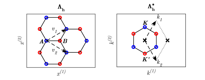
Figure 1. Left panel: ${\bf A}=(0,0)$, ${\bf B}=(\frac{1}{\sqrt{3}},0)$. Honeycomb structure, ${\bf H}$, is the union of two sub-lattices $\Lambda_{\bf A}={\bf A}+\Lambda_{h}$ (blue) and $\Lambda_{\bf B}={\bf B}+\Lambda_{h}$ (red); several hexagons shown. The lattice vectors $\{{\bf v}_{1},{\bf v}_{2}\}$ generate $\Lambda_{h}$. Right panel: Brillouin zone, ${\mathcal{B}}_{h}$, and dual basis $\{{\bf k}_{1},{\bf k}_{2}\}$. ${\bf K}$ and ${\bf K}^{\prime}$ are labeled.

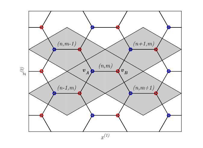
Figure 2. Four (shaded) tiles of a tiling of $\mathbb{R}^{2}$. These contain the lattice points, whose amplitudes couple to $\psi_{A}^{(n,m)}$ and $\psi_{B}^{(n,m)}$ according to the tight-binding model (1.1).

Figure 2 displays the honeycomb structure and several shaded cells of a tiling of $\mathbb{R}^{2}$ by diamond-shaped fundamental period cells. In each fundamental period cell, there are two atomic sites ($A-$ type and $B-$ type). Let $\left(\vec{\psi}_{A}(T),\vec{\psi}_{B}(T)\right)^{\rm t}=\left(\psi_{A}^{(n,m)}(T),\psi_{B}^{(n,m)}(T)\right)^{\rm t}_{(n,m)\in\mathbb{Z}^{2}}\in l^{2}(\mathbb{Z}^{2})\times l^{2}(\mathbb{Z}^{2})$ denote the time-dependent amplitudes of the ground states centered at the $A-$ and $B-$ sites of the cell with label $(n,m)$, i.e the period cell containing ${\bf v}_{A}+n{\bf v}_{1}+m{\bf v}_{2}$ and ${\bf v}_{B}+n{\bf v}_{1}+m{\bf v}_{2}$. Recall that modes of the full honeycomb structure are assumed to be superpositions of interacting lattice-translates of ground states, concentrated on the support of deep potential wells. Each $A$-site amplitude interacts with its three nearest neighbor $B$-site amplitudes, and analogously for each $B$-site amplitude. The discrete equations are:

$$i\partial_{T}\ \begin{bmatrix}\psi_{A}^{n,m}\\ \psi_{B}^{n,m}\ \end{bmatrix} =\ t\ \begin{bmatrix}\psi_{B}^{n,m}\ +\ \psi_{B}^{n,m-1}\ +\ \psi_{B}^{n-1,m}\\ \psi_{A}^{n,m}\ +\ \psi_{A}^{n+1,m}\ +\ \psi_{A}^{n,m+1}\end{bmatrix}$$

(1.1) $$=\ \frac{1}{|{\mathcal{B}}_{h}|}\ \int_{{\mathcal{B}}_{h}}\ e^{i{\bf k}\cdot(n{\bf v}_{1}+m{\bf v}_{2})}\ t\ H_{{}_{\rm TB}}({\bf k})\begin{bmatrix}\widehat{\psi}_{A}({\bf k})\\ \widehat{\psi}_{B}({\bf k})\end{bmatrix}\ d{\bf k}$$

where $t$ denotes a non-zero coupling (“hopping”) coefficient,

(1.2) $$H_{{}_{\rm TB}}({\bf k})\ \equiv\ \begin{pmatrix}0&-\overline{\gamma({\bf k})}\\ -\gamma({\bf k})&0\end{pmatrix},$$

(1.3) $$\gamma({\bf k})\ \equiv\ \sum_{\nu=1,2,3}e^{i{\bf k}\cdot{\bf e}_{B,\nu}}\ =\ e^{i{\bf k}\cdot{\bf e}_{B,1}}\ \left(\ 1\ +\ e^{i{\bf k}\cdot{\bf v}_{1}}\ +\ e^{i{\bf k}\cdot{\bf v}_{2}}\ \right)\quad\textrm{(see \eqref{gamma-def0})}\ ,$$

and $\left(\widehat{\psi}_{A}({\bf k}),\widehat{\psi}_{B}({\bf k})\right)^{\rm t}=\left(e^{-i{\bf k}\cdot({\bf e}_{B,1}/2)}\widetilde{\psi}_{A}({\bf k}),-e^{i{\bf k}\cdot({\bf e}_{B,1}/2)}\widetilde{\psi}_{B}({\bf k})\right)^{\rm t}$, where $\left(\widetilde{\psi}_{A}({\bf k}),\widetilde{\psi}_{B}({\bf k})\right)^{\rm t}$ denotes the discrete Fourier transform of $\left(\vec{\psi}_{A}(T),\vec{\psi}_{B}(T)\right)^{\rm t}$. The vectors ${\bf e}_{B,\nu},\nu=1,2,3$ are the three vectors directed from any point in $\Lambda_{B}$ to its three nearest neighbors in $\Lambda_{A}$, and analogously for ${\bf e}_{A,\nu},\nu=1,2,3$; see Figure 5 below.

Large but finite-time validity of such discrete approximations to time-dependent continuum Schrödinger equations, for certain initial data data, was studied in [ACZ:12, PSM:08].

The system (1.1) has two dispersion surfaces. To derive these explicitly, let $(\psi_{A}^{n,m},\psi_{B}^{n,m})^{\rm t}=(\alpha_{A},\alpha_{B})^{\rm t}e^{-i\mathcal{E}T}\ e^{i(n{\bf v}_{1}+m{\bf v}_{2})\cdot{\bf k}}$, where $\alpha_{A}$ and $\alpha_{B}$ are constants and ${\bf k}$ varies over the Brillouin zone, ${\mathcal{B}}_{h}$; see Figure 1 and Section 1.5. Substitution into (1.1) yields the dispersion relation for the two spectral bands of the tight-binding model:

$$\mathcal{E}_{\pm}({\bf k})\ =\ \pm\ |t|\ \mathscr{W}_{{}_{TB}}({\bf k})\ ,\ \ {\bf k}\in{\mathcal{B}}_{h}\ ,\ \ {\rm where}$$

(1.4) $$\mathscr{W}_{{}_{TB}}({\bf k}) \ \equiv\ |\gamma({\bf k})|\ =\ \left|\ 1+e^{i{\bf k}\cdot{\bf v}_{1}}+e^{i{\bf k}\cdot{\bf v}_{2}}\ \right|;$$

$\mathcal{E}_{\pm}({\bf k})$ are the two eigenvalue branches of $H_{{}_{\rm TB}}({\bf k})$. A plot of the two dispersion surfaces ${\bf k}\in\mathbb{R}^{2}\mapsto\ \mathcal{E}_{\pm}({\bf k}),\ \ {\bf k}\in{\mathcal{B}}_{h}$ is shown in Figure 3.

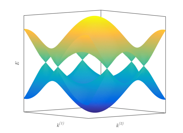
Figure 3. Dispersion surfaces of Wallace’s 2-band tight-binding model. Dispersion relation displayed in (1.4).

We note that the two dispersion surfaces are $\Lambda_{h}^{*}-$ periodic with respect to ${\bf k}$, and touch conically ($\mathscr{W}_{{}_{TB}}({\bf k})=0$) at the six vertices of ${\mathcal{B}}_{h}$, and their translates by the dual lattice, $\Lambda_{h}^{*}$; see Lemma 5.2. The energy / quasi-momentum pairs at these conical intersection points are so-called Dirac points; see Section 7.

1.3. Summary of results

We study the continuous Schrödinger operator, $-\Delta+\lambda^{2}V({\bf x})$, with honeycomb lattice potential, $V({\bf x})$, defined on $\mathbb{R}^{2}$ and $\lambda>\lambda_{\star}$ sufficiently large. Our particular model is one where $V$ is a superposition of “atomic” potential wells, $V_{0}({\bf x})$, supported within the union of discs, centered on points of the honeycomb structure, ${\bf H}$; see Figure 4. The detailed assumptions on $V_{0}({\bf x})$ (Section 4) ensure that $V({\bf x})$ is a honeycomb lattice potential in the sense of [FW:12], i.e. real-valued, periodic with respect equilateral triangular lattice, inversion symmetric and rotationally invariant by $120^{\circ}$.

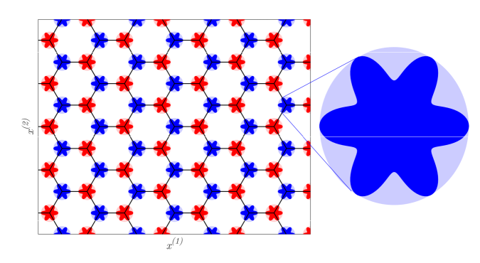
Figure 4. Lightly shaded discs of radius $r_{0}<\frac{1}{2}|{\bf e}_{A,1}|$, centered at each ${\bf v}\in{\bf H}=\Lambda_{A}\cup\Lambda_{B}$. A copy of the atomic potential $V_{0}$, satisfying hypotheses $(PW_{1})-(PW_{4})$, (GS) and (EG) in Section 4, is supported within each disc. The $60^{\circ}$ degree rotationally invariant support of $V_{0}$ is darkly shaded.

For ${\bf k}$ varying over the Brillouin zone, ${\mathcal{B}}_{h}$, let $E_{1}^{\lambda}({\bf k})\leq E^{\lambda}_{2}({\bf k})\leq\dots\leq E^{\lambda}_{b}({\bf k})\leq\dots$ (listed with multiplicity) denote the Floquet-Bloch spectrum of $-(\nabla+i{\bf k})^{2}+\lambda^{2}V({\bf x})$, considered with $\Lambda_{h}-$ periodic boundary conditions. The graphs of the mappings: ${\bf k}\mapsto E_{b}^{\lambda}({\bf k})$ are the dispersion surfaces. We study the following

Problem: Precisely describe the behavior of the dispersion surfaces of $-\Delta+\lambda^{2}V({\bf x})$, obtained from the low-lying (two lowest) eigenvalues of $-(\nabla+i{\bf k})^{2}+\lambda^{2}V({\bf x})$:

$${\bf k}\mapsto E_{1}^{\lambda}({\bf k})\ =\ E_{-}^{\lambda}({\bf k})\qquad{\rm and}\qquad{\bf k}\mapsto E_{2}^{\lambda}({\bf k})\ =\ E_{+}^{\lambda}({\bf k}),$$

for all $\lambda>\lambda_{\star}$ sufficiently large. This is called the regime of strong binding. We refer to the rescaled, $\lambda\to\infty$, limiting behavior as the tight-binding limit.

The Main Theorem, Theorem 6.1: For $\lambda>\lambda_{\star}$ sufficiently large, the rescaled low-lying dispersion surfaces, ${\bf k}\mapsto E^{\lambda}_{\pm}({\bf k})$, converge uniformly to Wallace’s (1947) two-band tight-binding model defined on a honeycomb structure. Specifically, for a suitable energy, $E^{\lambda}_{D}$, and $\rho_{\lambda}>0$, we have

(1.5) $$\left(\ E^{\lambda}_{-}({\bf k})-E^{\lambda}_{D}\ \right)/\rho_{\lambda}\to-\mathscr{W}_{{}_{TB}}({\bf k})\ \ {\rm and}\ \ \left(\ E^{\lambda}_{+}({\bf k})-E^{\lambda}_{D}\ \right)/\rho_{\lambda}\to+\mathscr{W}_{{}_{TB}}({\bf k})\ ,$$

as $$\lambda\to\infty {\bf k}\in{\mathcal{B}}_{h}$$, uniformly in , the Brillouin zone.

We also prove estimates and convergence of the derivatives of $E^{\lambda}_{\pm}({\bf k})$ on appropriate domains. Furthermore, in Theorem 6.2 we establish the scaled norm-convergence of the resolvent of $-\Delta+\lambda^{2}V$ to that of the tight-binding Hamiltonian, $H_{{}_{\rm TB}}$.

The first and second dispersion surfaces intersect precisely at the quasi-momenta located at the six vertices of $\mathcal{B}_{h}$ at the energy-level, $E_{D}^{\lambda}$. The parameter $\rho_{\lambda}$, displayed in (4.7), is given by an exponentially small overlap integral involving the atomic potential $V_{0}$, the ground state of $-\Delta+\lambda^{2}V_{0}$ and the ground state translated to a nearest neighbor site of ${\bf H}$; see Proposition 4.1.

Theorem 6.1 implies that, in the strong binding regime (all $\lambda$ sufficiently large), the only intersections of the lowest two dispersion surfaces occur at Dirac points, situated at the vertices, ${\bf K}_{\star}$, of ${\mathcal{B}}_{h}$. Moreover, (1.5) and the Taylor expansion of $\mathscr{W}_{{}_{TB}}({\bf k})$ (Lemma 5.2) near vertices gives:

(1.6) $$E_{\pm}^{\lambda}({\bf k})\ =\ E_{D}^{\lambda}\ \pm\ |{v^{\lambda}_{{}_{F}}}|\ |{\bf k}-{\bf K}_{\star}|+\mathcal{O}(\rho_{\lambda}|{\bf k}-{\bf K}_{\star}|^{2}),$$

where

(1.7) $$|{v^{\lambda}_{{}_{F}}}|\ =\ \left[\ \frac{\sqrt{3}}{2}+\mathcal{O}(e^{-c\lambda})\ \right]\rho_{\lambda}$$

is the Fermi velocity (see Definition 7.3 and [FW:12]), the velocity of “quasi-particles” (wave-packets) which are spectrally concentrated near Dirac points; see, for example, [RMP-Graphene:09, FW:14].

Remark 1.1 (Exchange of Dirac Points).

Consider the Schroedinger operator $-\Delta+\lambda^{2}V$. As in Theorem 6.1, we take $V({\bf x})$ to be a superposition of atomic wells $V_{0}({\bf x})$ centered at honeycomb lattice sites. As shown in Appendix A of [FLW-2d_edge:16] it is possible to choose $V_{0}({\bf x})$ so that $V_{{}_{1,1}}<0$, where $V_{{}_{1,1}}$ denotes the $(1,1)-$ Fourier coefficient of $V({\bf x})$. It follows from [FW:12] that for $\lambda$ sufficiently small and positive $-\Delta+\lambda^{2}V$ has Dirac points situated at the intersection of the $2^{nd}$ and $3^{rd}$ spectral bands. Furthermore, by Theorem 6.1 for $\lambda>\lambda_{\star}$ sufficiently large $-\Delta+\lambda^{2}V$ has Dirac points situated at the intersection of the $1^{st}$ and $2^{nd}$ spectral bands. It follows that for such honeycomb Schroedinger operators there is an exchange of Dirac points from the $2^{nd}$ and $3^{rd}$ bands to the $1^{st}$ and $2^{nd}$ bands as $\lambda$ is increased across a finite value of $\lambda=\lambda_{cr}$, where $0<\lambda_{cr}<\lambda_{\star}$. A further result in [FW:12] (see also Appendix D of [FLW-MAMS:17]) is that $-\Delta+\lambda^{2}V$ has Dirac points for all $\lambda>0$ outside a discrete set $\widetilde{C}$. Such examples prove that the exceptional set $\widetilde{C}$ can be non-empty.

Theorem 6.1, together with results in [FW:12] and [FLW-2d_edge:16], imply the following corollaries:

1. Corollary 6.3: Spectral gaps when breaking $\mathcal{P}\mathcal{T}$ symmetry. Honeycomb lattice potentials, $V$, have the property that the associated Schrödinger Hamiltonian, $-\Delta+\lambda^{2}V$, commutes with the composition of inversion with respect to an appropriate center, and complex conjugation, $\mathcal{C}\circ\mathcal{I}$. This is also known as $\mathcal{P}\mathcal{T}$ symmetry. For $\lambda$ large, a consequence of Theorem 6.1 and the results in [FW:12] is the existence of spectral gaps about Dirac points (see Section 7) of $-\Delta+\lambda^{2}V$ when the Hamiltonian is perturbed in such a way as to break $\mathcal{P}\mathcal{T}$ symmetry.

   A review of other mechanisms for construction spectral gaps, also in the high-contrast regime, appears in [Hempel-Post:03]; see also [Figotin-Kuchment:96a, Figotin-Kuchment:96b].

2. Corollary 6.4: Protected edge states in honeycomb structures with line-defects. Edge states are time-harmonic solutions of the Schrödinger equation, which are propagating parallel to a line-defect (edge) and are localized transverse to it; see Figure 7. In [FLW-2d_edge:16] (see also [FLW-2d_materials:15]), we develop a theory of protected edge states for honeycomb structures, perturbed by a class of line-defects (domain walls) in the direction of an element of $\Lambda_{h}$ (rational edges). The key hypothesis is a spectral no-fold condition. Our main result, Theorem 6.1, implies the validity of the spectral no-fold condition, and hence the existence of edge states for a large class of rational edges, in the strong binding regime.

   Previous analytical work on topologically protected edge states in periodic structures with line-defects has focused on approximate tight-binding models; see, for example, [RMP-Graphene:09, delplace2011zak, Graf-Porta:13].

   Finally, we remark that the effect of interacting electrons in graphene, in the tight-binding limit, have been studied in [Giuliani-Mastropietro:10, Giuliani-Mastropietro-Porta:12].

1.4. Outline

In Section 2 we review basic Floquet-Bloch theory of Schrödinger operators with periodic potentials. Section 3 introduces the honeycomb structure, ${\bf H}$, which is the union of the two sublattices $\Lambda_{A}$ and $\Lambda_{B}$. Section 4 discusses hypotheses on the atomic potential well, $V_{0}$, and Section 5 treats its $\Lambda_{h}-$ periodization, $V$, obtained via summation over translates by vectors ${\bf v}\in{\bf H}$. The atomic potential, $V_{0}$, is assumed to have compact support, $|{\bf x}|<r_{0}$, where $r_{0}<r_{critical}$ and $r_{critical}$ (which is less than than half the distance nearest neighbor lattice points in ${\bf H}$) is determined by a Geometric Lemma presented in Section 15. The assertions of this lemma are easily seen to hold for $r_{0}$ positive and sufficiently small. A non-trivial lower bound for $r_{critical}$ is of interest in applications and for this we require the Geometric Lemma.

In Section 6 we state our main result, Theorem 6.1, on the low-lying dispersion surfaces of $-\Delta+\lambda^{2}V$, for $\lambda>\lambda_{\star}$ sufficiently large. We also state and prove consequences for Schrödinger operators on $\mathbb{R}^{2}$ with perturbed honeycomb structures in the regime of strong binding: Corollary 6.3 on spectral gaps and Corollary 6.4 on protected edge states.

Section 7 reviews the notion of Dirac points and results on the existence of Dirac points for generic honeycomb lattice potentials [FW:12, FLW-MAMS:17]; see also [Colin-de-Verdiere:91, Grushin:09, berkolaiko-comech:15, Lee:16]. Dirac points are energy / quasi-momentum pairs, which occur at quasi-momenta located at the vertices of the Brillouin zone, ${\mathcal{B}}_{h}$, and at which neighboring dispersion surfaces touch conically. For an extensive discussion of Dirac points and edge states for nanotube structures in the context of quantum graphs, see [Kuchment-Post:07] and [Do-Kuchment:13].

The proof of the main theorem, Theorem 6.1, on the large $\lambda$ behavior of low-lying dispersion surfaces is carried out in Sections 8 through 15. In Section 8 we construct approximate Floquet-Bloch modes, $p^{\lambda}_{{\bf k},A}({\bf x})$ and $p^{\lambda}_{{\bf k},B}({\bf x})$ (associated with the sublattices $\Lambda_{A}$ and $\Lambda_{B}$) for the two lowest spectral bands of the Floquet-Bloch Hamiltonian $H^{\lambda}({\bf k})=-(\nabla_{\bf x}+i{\bf k})^{2}+\lambda^{2}V({\bf x})-E_{0}^{\lambda}$ ( ${\bf k}\in\mathbb{R}^{2}$), in terms of the ground state eigenpair, $\left(E_{0}^{\lambda},p_{0}^{\lambda}({\bf x})\right)$, of the atomic Hamiltonian, $-\Delta+\lambda^{2}V_{0}$.

In Section 9 we first derive energy estimates for the family of Floquet-Bloch Hamiltonians $H^{\lambda}({\bf k})=-(\nabla_{\bf x}+i{\bf k})^{2}+\lambda^{2}V({\bf x})-E_{0}^{\lambda}$, ${\bf k}\in\mathbb{R}^{2}$, restricted to the $L^{2}(\mathbb{R}^{2}/\Lambda_{h})-$ orthogonal complement of these approximate Floquet-Bloch modes. We then use these estimates to prove resolvent bounds on this subspace.

In Sections 10 through 15 we apply resolvent bounds on $H^{\lambda}({\bf k})$, in a Lyapunov-Schmidt reduction scheme, for $\lambda$ large, to the 2D subspace ${\rm span}\{p^{\lambda}_{{\bf k},A}({\bf x}),p^{\lambda}_{{\bf k},B}({\bf x})\}$. The main steps are (i) a proof of key properties of Dirac points at the vertices of the Brillouin zone, ${\mathcal{B}}_{h}$ (Theorem 10.1) and (ii) a study of uniform convergence of the (rescaled) low-lying dispersion maps ${\bf k}\mapsto E^{\lambda}_{\pm}({\bf k})$ to the dispersion surfaces of Wallace’s tight-binding model (Propositions 14.1 and 14.3).

In Section 11 we characterize the low-lying dispersion surfaces as the locus of points, $(\Omega,{\bf k})\in\mathbb{R}\times\mathbb{R}^{2}$ satisfying $\det\mathcal{M}^{\lambda}(\Omega,{\bf k})=0$. For each $\lambda$ sufficiently large $(\Omega,{\bf k})\mapsto\mathcal{M}^{\lambda}(\Omega,{\bf k})$ is an analytic map from a subset $U\subset\mathbb{C}\times\mathbb{C}^{2}$ into the space of $2\times 2$ matrices, where $\mathcal{M}^{\lambda}(\Omega,{\bf k})$ is Hermitian for real $\Omega$ and ${\bf k}$. In Section 12 we expand $\mathcal{M}^{\lambda}(\Omega,{\bf k})$ for large $\lambda$ and in Sections 13 and 14 we introduce and analyze a rescaling of $\det\mathcal{M}^{\lambda}(\Omega,{\bf k})$ to complete the proof of our main result, Theorem 6.1.

Section 15 contains estimates that facilitate our control of the large $\lambda-$ perturbation theory in terms of an intrinsic (exponentially small) parameter, $\rho_{\lambda}$. This parameter has the form of an integral of the product of: the atomic potential well $V_{0}({\bf x})$, the atomic ground state, $p_{0}^{\lambda}({\bf x})$, and the translate of $p_{0}^{\lambda}({\bf x})$ to a nearest neighbor lattice site in ${\bf H}$. An important tool is a lemma in Euclidean geometry, used to bound the ground state $-\Delta+\lambda^{2}V_{0}({\bf x})$ and to quantify the maximum allowable size of the support of the atomic potential well in our proofs.

In the remainder of this section we discuss some definitions, notation and conventions used throughout the paper.

1.5. Notations and conventions

We denote by $\Lambda_{h}=\mathbb{Z}{\bf v}_{1}\oplus\mathbb{Z}{\bf v}_{2},$ the equilateral triangular lattice generated by the basis vectors:

(1.14) $${\bf v}_{1} =\ \left(\begin{array}[]{c}\frac{\sqrt{3}}{2}\\ {}\hfil\\ \frac{1}{2}\end{array}\right),\ \ {\bf v}_{2}=\ \left(\begin{array}[]{c}\frac{\sqrt{3}}{2}\\ {}\hfil\\ -\frac{1}{2}\end{array}\right)\ .$$

The dual lattice $\Lambda_{h}^{*}=\ \mathbb{Z}{\bf k}_{1}\oplus\mathbb{Z}{\bf k}_{2}$ is spanned by the dual basis vectors:

(1.21) $${\bf k}_{1}=\ 2\pi\left(\begin{array}[]{c}\frac{\sqrt{3}}{3}\\ {}\hfil\\ 1\end{array}\right),\ \ \ {\bf k}_{2}=2\pi\left(\begin{array}[]{c}\frac{\sqrt{3}}{3}\\ {}\hfil\\ -1\end{array}\right).\$$

Note that ${\bf k}_{\ell}\cdot{\bf v}_{{\ell^{\prime}}}=2\pi\delta_{\ell{\ell^{\prime}}}$. The Brillouin zone, ${\mathcal{B}}_{h}$, is the hexagon in $\mathbb{R}^{2}_{\bf k}$ consisting of all points which are closer to the origin than to any other point in $\Lambda_{h}^{*}$; see Figure 1.

Denote by ${\bf K}$ and ${\bf K^{\prime}}$ the vertices of ${\mathcal{B}}_{h}$ given by:

(1.22) $${\bf K}\equiv\frac{1}{3}\left({\bf k}_{1}-{\bf k}_{2}\right)=\begin{pmatrix}0\\ \frac{4\pi}{3}\end{pmatrix},\ \ {\bf K^{\prime}}\equiv-{\bf K}\ .$$

All six vertices of ${\mathcal{B}}_{h}$ can be generated from ${\bf K}$ and ${\bf K}^{\prime}$ by application of the rotation matrix, $R$, which rotates a vector in $\mathbb{R}^{2}$ clockwise by $2\pi/3$ about the origin. The matrix $R$ is given by

(1.23) $$R\ =\ \left(\begin{array}[]{cc}-\frac{1}{2}&\frac{\sqrt{3}}{2}\\ {}\hfil&{}\hfil\\ -\frac{\sqrt{3}}{2}&-\frac{1}{2}\end{array}\right)$$

Note the relations:

$$R^{*}{\bf v}_{1}\ =\ -{\bf v}_{2},\qquad R^{*}{\bf v}_{2}\ =\ {\bf v}_{1}-{\bf v}_{2}$$

In Section 3 we make the choice of diamond-shaped fundamental cell for the honeycomb structure, $D$, shown in Figure 5. $D$ contains two base-points ,

(1.24) $${\bf v}_{A}\ =\ \begin{pmatrix}0\\ 0\end{pmatrix},\qquad{\bf v}_{B}\ =\ \begin{pmatrix}\frac{1}{\sqrt{3}}\\ 0\end{pmatrix},$$

of the sublattices, $\Lambda_{A}$ and $\Lambda_{B}$, which comprise the honeycomb structure. The location

(1.25) $${\bf x}_{c}\ =\ \frac{1}{2}\ \begin{pmatrix}\frac{1}{\sqrt{3}}\\ -1\end{pmatrix}\ .$$

marks the center of a hexagon and is a vertex of $D$.

Additional frequently used notations and conventions are:

1. For ${\bf m}=(m_{1},m_{2})\in\mathbb{Z}^{2}$, ${\bf m}\vec{\bf k}=m_{1}{\bf k}_{1}+m_{2}{\bf k}_{2}$ and ${\bf m}\vec{\bf v}=m_{1}{\bf v}_{1}+m_{2}{\bf v}_{2}$.

2. ${\bf k}=(k^{(1)},k^{(2)})$.

3. ${\tilde{\bf K}}$ will be used to denote a generic quasi-momentum.

4. ${\bf K}_{\star}$ will be used to denote for a generic element of $\Lambda_{\bf K}^{*}\cup\Lambda_{{\bf K}^{\prime}}^{*}=\left({\bf K}+\Lambda_{h}^{*}\right)\cup\left({\bf K}^{\prime}+\Lambda_{h}^{*}\right)$. These are the vertices of the Brillouin zone, $\mathcal{B}_{h}$, and their translates by the dual lattice.

5. $E_{D}^{\lambda}$ or $E_{D}$ denotes the energy of a Dirac point.

6. $x\lesssim y$ if and only if there exists $C>0$ such that $x\leq Cy$. And $x\approx y$ if and only if $x\lesssim y$ and $y\lesssim x$. We shall discuss below the dependencies of constants $C$.

7. $\left\langle f,g\right\rangle$ is an inner product, which is linear in $g$ for fixed $f$, and conjugate linear in $f$, for fixed $g$.

8. Let $\Lambda$ denote an arbitrary lattice in the plane, $\mathbb{R}^{2}$. For $s\in\mathbb{R}$, the space $H^{s}(\mathbb{R}^{2}/\Lambda)$ consists of complex-valued and $\Lambda-$ periodic functions $f$ on $\mathbb{R}^{2}$, whose Fourier coefficients, $\{\widehat{f}({\bf m})\}_{{}_{{\bf m}\in\mathbb{Z}^{2}}}$, satisfy

   $$\|f\|_{{}_{H^{s}(\mathbb{R}^{2}/\Lambda)}}^{2}\ \equiv\ \sum_{{\bf m}\in\mathbb{Z}^{2}}(1+|{\bf m}|^{2})^{s}\ |\widehat{f}({\bf m})|^{2}\ <\ \infty\ .$$

9. For ${\bf F}=(F_{1},F_{2},\dots,F_{m})$, with each $F_{j}\in\mathcal{Y}$, a normed linear space, we write $\|{\bf F}\|_{{}_{\mathcal{Y}}}=\sum_{j=1}^{m}\|F_{j}\|_{{}_{\mathcal{Y}}}$.

We study $-\Delta+\lambda^{2}V_{0}({\bf x})$ and its $\Lambda_{h}-$ periodic variants. Here, $\lambda>0$ is a coupling constant, assumed to satisfy $\lambda>\lambda_{\star}$ for a large enough $\lambda_{\star}$; and $V_{0}({\bf x})$ is a given potential defined on $\mathbb{R}^{2}$. We write $c,C,C^{\prime}$ etc. to denote constants which depend on $V_{0}$. A discussion of the precise dependencies of constants is given in Section 17. These symbols may denote different constants in different occurrences. As a result of the above conventions, it is correct to assert, for example, $\lambda^{10}e^{-c\lambda}\leq e^{-c\lambda}$.

Finally, for relations involving norms and inner products in which we do not explicitly indicate the relevant function space, it is to be understood that these are taken in $L^{2}(\mathbb{R}^{2}/\Lambda_{h})$.

1.6. Acknowledgements

The authors thank G. Berkolaiko for his interest and feedback concerning this work. We thank the referee for a careful reading and incisive comments which, in particular, inspired Theorem 6.2 and Section 16. This research was supported in part by National Science Foundation grants DMS-1265524 (CLF) and DMS-1412560 (MIW & JPL-T) and Simons Foundation Math + X Investigator Award #376319 (MIW).

2. Floquet-Bloch Theory and Honeycomb Lattice Potentials

We begin with a review of Floquet-Bloch theory. For the theory, see [Eastham:74, Kuchment:12, Kuchment:16, RS4] and [avron-simon:78, Skriganov:85, Gerard:90, Karpeshina:97, Gerard-Nier:98].

2.1. Fourier analysis on $L^{2}(\mathbb{R}/\Lambda)$

Let $\{{\bm{\mathfrak{v}}}_{1},{\bm{\mathfrak{v}}}_{2}\}$ be a linearly independent set in $\mathbb{R}^{2}$, and introduce the

$$\text{\bf Lattice: }\Lambda=\mathbb{Z}{\bm{\mathfrak{v}}}_{1}\oplus\mathbb{Z}{\bm{\mathfrak{v}}}_{2}=\{m_{1}{\bm{\mathfrak{v}}}_{1}+m_{2}{\bm{\mathfrak{v}}}_{2}\ :\ m_{1},m_{2}\in\mathbb{Z}\};$$

$$\text{\bf Dual lattice: }\Lambda^{\ast}=\mathbb{Z}{\bm{\mathfrak{K}}}_{1}\oplus\mathbb{Z}{\bm{\mathfrak{K}}}_{2}=\{{\bf m}\vec{\bm{\mathfrak{K}}}=m_{1}{\bm{\mathfrak{K}}}_{1}+m_{2}{\bm{\mathfrak{K}}}_{2}:m_{1},m_{2}\in\mathbb{Z}\},$$

$$\qquad\qquad\qquad\qquad\qquad{\bm{\mathfrak{K}}}_{i}\cdot{\bm{\mathfrak{v}}}_{j}=2\pi\delta_{ij},\ 1\leq i,j\leq 2;$$

$$\text{\bf Fundamental period cell, }\ \Omega\subset\mathbb{R}^{2};$$

$$\text{\bf Brillouin zone: }\mathcal{B},\ \textrm{a choice of fundamental dual cell}.$$

Definition 2.1 (The spaces $L^{2}(\mathbb{R}^{2}/\Lambda)$ and $L^{2}_{\bf k}$).

1. $L^{2}(\mathbb{R}^{2}/\Lambda)$ denotes the space of $L^{2}_{loc}$ functions which are $\Lambda-$ periodic: $f\in L^{2}(\mathbb{R}^{2}/\Lambda)$ if and only if $f({\bf x}+{\bm{\mathfrak{v}}})=f({\bf x})$ for almost all ${\bf x}\in\mathbb{R}^{2},\ {\bm{\mathfrak{v}}}\in\Lambda$; and $f\in L^{2}(\Omega)$.

2. $L^{2}_{\bf k}$ denotes the space of $L^{2}_{loc}$ functions which satisfy a pseudo-periodic boundary condition: $f({\bf x}+{\bm{\mathfrak{v}}})=e^{i{\bf k}\cdot{\bm{\mathfrak{v}}}}f({\bf x})$ for all ${\bm{\mathfrak{v}}}\in\Lambda$ and almost all ${\bf x}\in\mathbb{R}^{2}$; i.e. $e^{-i{\bf k}\cdot{\bf x}}f({\bf x})\in L^{2}(\mathbb{R}^{2}/\Lambda)$.

   For $f$ and $g$ in $L^{2}_{\bf k}$, $\overline{f}g$ is in $L^{2}(\mathbb{R}^{2}/\Lambda)$ and we define the inner product by

   $$\left\langle f,g\right\rangle_{L^{2}_{\bf k}}=\int_{\Omega}\overline{f({\bf x})}g({\bf x})d{\bf x}.$$

2.2. Floquet-Bloch theory

Let $Q({\bf x})$ denote a real-valued potential which is periodic with respect to $\Lambda$. We shall assume throughout this paper that $Q\in C^{\infty}(\mathbb{R}^{2}/\Lambda)$, although we expect that this condition can be relaxed significantly without much extra work; see Remark 4.1. Introduce the Schrödinger Hamiltonian $H\equiv-\Delta+Q({\bf x})$. For each ${\bf k}\in\mathbb{R}^{2}$, we study the Floquet-Bloch eigenvalue problem on $L^{2}_{\bf k}$:

(2.1) $$H\Phi({\bf x};{\bf k})=E({\bf k})\Phi({\bf x};{\bf k}),\ \ {\bf x}\in\mathbb{R}^{2},$$

$$\Phi({\bf x}+{\bm{\mathfrak{v}}};{\bf k})=e^{i{\bf k}\cdot{\bm{\mathfrak{v}}}}\Phi({\bf x};{\bf k}),\ \ {\bm{\mathfrak{v}}}\in\Lambda.$$

An $L^{2}_{\bf k}-$ solution of (2.1) is called a Floquet-Bloch state.

Since the ${\bf k}-$ pseudo-periodic boundary condition in (2.1) is invariant under translations in the dual period lattice, $\Lambda^{\ast}$, it suffices to restrict our attention to ${\bf k}\in\mathcal{B}$, where $\mathcal{B}$, the Brillouin Zone, is a fundamental cell in ${\bf k}-$ space.

An equivalent formulation to (2.1) is obtained by setting $\Phi({\bf x};{\bf k})=e^{i{\bf k}\cdot{\bf x}}p({\bf x};{\bf k})$. Then,

(2.2) $$H({\bf k})p({\bf x};{\bf k})=E({\bf k})p({\bf x};{\bf k}),\ {\bf x}\in\mathbb{R}^{2},\quad p({\bf x}+{\bm{\mathfrak{v}}})=p({\bf x};{\bf k}),\ \ {\bm{\mathfrak{v}}}\in\Lambda,$$

where $H({\bf k})\equiv-(\nabla+i{\bf k})^{2}+Q({\bf x})$ is a self-adjoint operator on $L^{2}(\mathbb{R}^{2}/\Lambda)$. The eigenvalue problem (2.2), has a discrete set of eigenvalues $E_{1}({\bf k})\leq E_{2}({\bf k})\leq\cdots\leq E_{b}({\bf k})\leq\cdots$, with $L^{2}(\mathbb{R}^{2}/\Lambda)-$ eigenfunctions $p_{b}({\bf x};{\bf k}),\ b=1,2,3,\ldots$. The maps ${\bf k}\in\mathcal{B}\mapsto E_{j}({\bf k})$ are, in general, Lipschitz continuous functions; for example, see [avron-simon:78, Kuchment:12, Kuchment:16] and Appendix A of [FW:14]. For each ${\bf k}\in\mathcal{B}$, the set $\{p_{j}({\bf x};{\bf k})\}_{j\geq 1}$ can be taken to be a complete orthonormal basis for $L^{2}(\mathbb{R}^{2}/\Lambda)$.

As ${\bf k}$ varies over $\mathcal{B}$, $E_{b}({\bf k})$ sweeps out a closed interval in $\mathbb{R}$. The union over $b\geq 1$ of these closed intervals is exactly the $L^{2}(\mathbb{R}^{2})-$ spectrum of $-\Delta+Q({\bf x})$: $\text{spec}\left(H\right)=\bigcup_{{\bf k}\in\mathcal{B}}\text{spec}\left(H({\bf k})\right).$ Furthermore, the set $\{\Phi_{b}({\bf x};{\bf k})\}_{b\geq 1,{\bf k}\in\mathcal{B}}$ is complete in $L^{2}(\mathbb{R}^{2})$. For a suitable normalization of $\Phi_{b}({\bf x};{\bf k})$, we have

$$f({\bf x})=\sum_{b\geq 1}\int_{\mathcal{B}}\left\langle\Phi_{b}(\cdot;{\bf k}),f(\cdot)\right\rangle_{L^{2}(\mathbb{R}^{2})}\Phi_{b}({\bf x};{\bf k})d{\bf k}\equiv\sum_{b\geq 1}\int_{\mathcal{B}}\widetilde{f}_{b}({\bf k})\Phi_{b}({\bf x};{\bf k})d{\bf k},$$

where the sum converges in the $L^{2}$ norm.

3. Honeycomb Structure

Denote by $\Lambda_{h}\subset\mathbb{R}^{2}$, the equilateral triangular lattice specified in Section 1.5. Recall the base points ${\bf v}_{A}$ and ${\bf v}_{B}$, defined in (1.24).

Sublattices: $\Lambda_{A}$ and $\Lambda_{B}$ and the honeycomb structure ${\bf H}$: Generate the $A-$ sublattice, $\Lambda_{A}$, and the $B-$ sublattice, $\Lambda_{B}$: $\Lambda_{I}={\bf v}_{I}+\Lambda_{h}\subset\mathbb{R}^{2},\ \ I=A,B$ . The honeycomb structure is defined to be:

$${\bf H}=\Lambda_{A}\ \cup\ \Lambda_{B}\subset\mathbb{R}^{2}.$$

$D$, fundamental domain for $\mathbb{R}^{2}/\Lambda_{h}$: Let $D\subset\mathbb{R}^{2}$ denote the diamond-shaped fundamental domain for the torus, $\mathbb{R}^{2}/\Lambda_{h}$, shown in Figure 5. Choose $D$ so that ${\bf v}_{A},{\bf v}_{B}\in D$. ${\bf x}_{c}$ is the center of a hexagon (not a point in ${\bf H}$) and a vertex of the parallelogram $D$. For any $F\in L^{1}(\mathbb{R}^{2})$ we have

$$\int_{{\bf x}\in\mathbb{R}^{2}}\ F({\bf x})\ d{\bf x}\ =\ \int_{{\bf x}\in D}\ \sum_{{\bf v}\in\Lambda_{h}}F({\bf x}-{\bf v})\ d{\bf x}.$$

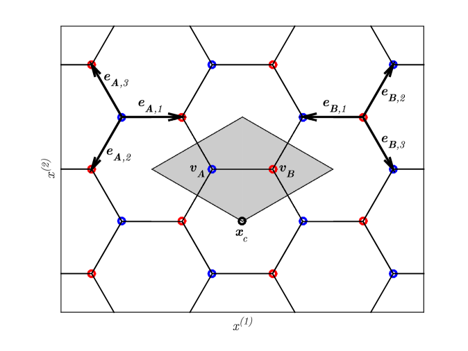
Figure 5. Diamond-shaped (shaded) fundamental domain, $D$, containing two base points of the honeycomb, ${\bf H}$: ${\bf v}_{A}=(0,0)$ and ${\bf v}_{B}=(1/\sqrt{3},0)$. Hexagon center, ${\bf x}_{c}$, is a point relative to which the honeycomb potential $V$ is $120^{\circ}$ rotationally invariant and inversion symmetric. Indicated are: vectors ${\bf e}_{A,\nu},\ \nu=1,2,3$ from a typical site in $\Lambda_{A}$ pointing to its three nearest neighbors in $\Lambda_{B}$, and ${\bf e}_{B,\nu}=-{\bf e}_{A,\nu},\ \nu=1,2,3$ from a site typical $\Lambda_{B}$ pointing to its three nearest neighbors in $\Lambda_{A}$.

Nearest neighbors in ${\bf H}$: For any fixed ${\bf v}\in\Lambda_{A}$, the points in ${\bf H}$ which are nearest to ${\bf v}$ are the three points in the lattice $\Lambda_{B}$ given by:

(3.1) $${\bf v}+{\bf e}_{A,1},\ {\bf v}+{\bf e}_{A,2},\ {\rm and}\ {\bf v}+{\bf e}_{A,3}.$$

Here ${\bf e}_{A,\nu},\ \nu=1,2,3$ are shown in Figure 5. Thus,

(3.2) $${\bf e}_{A,\nu}=R^{\nu-1}{\bf e}_{A,1}=R^{\nu-1}\begin{pmatrix}\frac{1}{\sqrt{3}}\\ 0\end{pmatrix},\ \ \nu=1,2,3,$$

where $R$ is the $120^{\circ}$ clockwise rotation matrix; see (1.23).

Similarly, for any ${\bf w}\in\Lambda_{B}$, the points in ${\bf H}$ which are nearest to ${\bf w}$ are the three points in $\Lambda_{A}$:

(3.3) $${\bf w}+{\bf e}_{B,1},\ {\bf w}+{\bf e}_{B,2},\ {\rm and}\ {\bf w}+{\bf e}_{B,3},$$

where ${\bf e}_{B,\nu},\ \nu=1,2,3$ are shown in Figure 5. Note that ${\bf e}_{A,\nu}=-{\bf e}_{B,\nu}$.

4. Atomic potential well, $V_{0}({\bf x})$, and ground state: $(p_{0}^{\lambda}({\bf x}),E_{0}^{\lambda})$

Fix a smooth potential well $V_{0}({\bf x})$ on $\mathbb{R}^{2}$ with the following properties.

• $-1\leq V_{0}({\bf x})\leq 0,\ {\bf x}\in\mathbb{R}^{2}$.

• support $V_{0}\ \subset\ \{{\bf x}\in\mathbb{R}^{2}:|{\bf x}|<r_{0}\}$, where $r_{0}<r_{critical}$. Here,

  $$0.33|{\bf e}_{A,1}|\leq r_{critical}<0.5|{\bf e}_{A,1}|,\$$

  as determined in Geometric Lemma 15.1, and $|{\bf e}_{A,1}|=1/\sqrt{3}$ is the distance between nearest neighbor vertices.

• $V_{0}({\bf x})$ is invariant under a $2\pi/3$ ($120^{\circ}$) rotation about the origin, ${\bf x}=0$.

• $V_{0}({\bf x})$ is inversion-symmetric with respect to the origin; $V_{0}(-{\bf x})=V_{0}({\bf x})$.

Consider the “atomic” Schrödinger operator $-\Delta+\lambda^{2}V_{0}({\bf x})$ in $L^{2}(\mathbb{R}^{2})$. Let $p_{0}^{\lambda}({\bf x}),E_{0}^{\lambda}$, respectively, be the ground state eigenfunction and strictly negative ground state eigenvalue of $-\Delta+\lambda^{2}V_{0}({\bf x})$. This eigenpair is simple and, by the symmetries of $V_{0}$, $p_{0}^{\lambda}({\bf x})$ is invariant under a $60^{\circ}$ rotation about the origin.

We normalize $p_{0}^{\lambda}({\bf x})$ so that $p_{0}^{\lambda}({\bf x})>0$ for all ${\bf x}\in\mathbb{R}^{2}$, and

$$\int_{\mathbb{R}^{2}}|\ p_{0}^{\lambda}({\bf x})\ |^{2}\ d{\bf x}\ =\ 1.$$

Note that since $V_{0}\in L^{\infty}(\mathbb{R}^{2})$, $p_{0}^{\lambda}\in H^{2}(\mathbb{R}^{2})$. The ground state, $p_{0}^{\lambda}$, satisfies the following pointwise bound

(4.1) $$p_{0}^{\lambda}({\bf x}) \leq\begin{cases}C_{1}\ e^{-c_{1}\lambda|{\bf x}|},&|{\bf x}|\geq r_{0}+c_{0}\\ C_{2}\ \lambda,&|{\bf x}|<r_{0}+c_{0}.\end{cases}$$

where $\text{supp}(V_{0})\subset B(0,r_{0})$ and $c_{0}>0$, and $C_{1},C_{2}$ and $c_{1}$ are constants that depend on $V_{0}$, $r_{0}$ and $c_{0}$; see Corollary 15.5.

In addition to hypotheses $(PW_{1})-(PW_{4})$ on $V_{0}({\bf x})$, we assume the following two properties of the Hamiltonian $-\Delta+\lambda^{2}V_{0}({\bf x})$:

(GS) Ground state energy upper bound: For $\lambda$ large, $E_{0}^{\lambda}$, the ground state energy of $-\Delta+\lambda^{2}V_{0}({\bf x})$, satisfies the upper bound

(4.2) $$E_{0}^{\lambda}\ \leq\ -C\lambda^{2}.$$

Here, $C$ is a strictly positive constant depending on $V_{0}$. A simple consequence of the variational characterization of $E_{0}^{\lambda}$ is the lower bound $E_{0}^{\lambda}\geq-\|V_{0}\|_{{}_{L^{\infty}}}\lambda^{2}=-\lambda^{2}$. However, the upper bound (4.2) requires further restrictions on $V_{0}$.

(EG) Energy gap property: There exists $c_{gap}>0$, such that if $\psi\in H^{2}(\mathbb{R}^{2})$ and $\left\langle p_{0}^{\lambda},\psi\right\rangle_{{}_{L^{2}(\mathbb{R}^{2})}}=\ 0$, then

(4.3) $$\left\langle\ \left(-\Delta+\lambda^{2}V_{0}\right)\psi,\psi\ \right\rangle_{{}_{L^{2}(\mathbb{R}^{2})}}\ \geq\ (E_{0}^{\lambda}+c_{gap})\ \|\psi\|_{{}_{L^{2}(\mathbb{R}^{2})}}^{2}.$$

4.1. Examples of the energy gap property, (EG)

1. Let $V_{0}({\bf x})$ be a smooth potential well. For simplicity, assume that $V_{0}$ has a single non-degenerate minimum at ${\bf x}={\bf 0}$: $\min_{{}_{{\bf x}\in\mathbb{R}^{2}}}V_{0}({\bf x})=V_{0}({\bf 0})=-1$, $D^{2}V({\bf 0})=I$, $-1\leq V_{0}({\bf x})\leq 0$ and $V_{0}({\bf x})\to 0$ sufficiently rapidly as $|{\bf x}|\to\infty$. Then, a simple argument based on the scaling: ${\bf y}=\lambda^{1\over 2}{\bf x}$, indicates that for fixed $N\geq 1$ and $\lambda>\lambda_{N}$ sufficiently large, the first $N-$ eigenvalues of $-\Delta_{\bf x}+\lambda^{2}V_{0}({\bf x})$ satisfy, to leading order:

   (4.4) $$E_{j}^{\lambda}\ =\ -\lambda^{2}+\lambda\ h_{j},\ \ 1\leq j\leq N,$$

   where $h_{j}$ is the $j^{th}$ eigenvalue of the harmonic oscillator Hamiltonian $-\Delta_{\bf y}+\frac{1}{2}|{\bf y}|^{2}$. Rigorous results are presented in [Simon:83, CFKS:87]. In this case we have that $c_{gap}$ is of order $\lambda$.

2. Consider piecewise constant cylindrical well, defined by the potential

   (4.5) $$V_{0}({\bf x})=\begin{cases}-1&\textrm{ for $|{\bf x}|<R$}\\ 0&\textrm{ for $|{\bf x}|\geq R$}\end{cases}$$

   (Strictly speaking this choice of $V_{0}$ does not satisfy the above smoothness hypotheses, but it is not difficult to extend our conclusions concerning $c_{gap}$, to the case where the discontinuity of $V_{0}$ is smoothed out.) Solutions which are regular at $|{\bf x}|=0$ and are decaying as $|{\bf x}|\to\infty$ are of the form $e^{im\theta}u(r)$, where

   $$u(r)=\begin{cases}\alpha_{0}\ J_{m}(\sqrt{\lambda^{2}-|E|}\ |{\bf x}|)&\textrm{ for $|{\bf x}|\leq R$}\\ \alpha\ I_{m}(|E|^{\frac{1}{2}}|{\bf x}|)&\textrm{ for $|{\bf x}|>R$}.\end{cases}$$

   Here, $J_{m}(r)$ and $I_{m}(r)$ are respectively the Bessel and modified Bessel functions of order $m\geq 0$; $J_{m}(r)$ is regular at $r=0$ and $I_{m}(r)$ decays exponentially as $r\to\infty$. Eigenvalues, $E$, are given by solutions of

   (4.6) $$J_{m}(\sqrt{\lambda^{2}-|E|}\ R)=\frac{\sqrt{\lambda^{2}-|E|}}{|E|^{1\over 2}}\ \frac{I_{m}^{\prime}(|E|^{1\over 2})}{I_{m}(|E|^{1\over 2})}\ J_{m}^{\prime}(\sqrt{\lambda^{2}-|E|}\ R),$$

   Consider say the first two eigenvalues of $-\Delta+\lambda^{2}V_{0}({\bf x})$. For $\lambda$ sufficiently large, these eigenvalues are given, to leading order by: $E=-\lambda^{2}+\left(\rho/R\right)^{2}$, where $\rho$ varies over the roots of $J_{m}(\rho)=0$. Therefore, in this case $c_{gap}$ is of order $1$.

4.2. Bounds on the derived (intrinsic) small parameter, $\rho_{\lambda}$

Let

(4.7) $$\rho_{\lambda}\ \equiv\ \int\lambda^{2}|V_{0}({\bf y})|\ p_{0}^{\lambda}({\bf y})\ p_{0}^{\lambda}({\bf y}+{\bf e}_{A,1})\ d{\bf y}\ .$$

Proposition 4.1.

There exist positive constants $\lambda_{\star}$, $c_{1}$ and $c_{2}$, all depending on $V_{0}$, such that for all $\lambda>\lambda_{\star}$,

(4.8) $$e^{-c_{1}\lambda}\ \lesssim\ \rho_{\lambda}\ \lesssim\ \ e^{-c_{2}\lambda}$$

The proof is given in Section 15.

Remark 4.2.

By hypotheses $(PW_{1})-(PW_{4})$ on $V_{0}$, the expression $\int\lambda^{2}|V_{0}({\bf y})|\ p_{0}^{\lambda}({\bf y})\ p_{0}^{\lambda}({\bf y}+{\bf e}_{I,\nu})\ d{\bf y}$ is independent of $I\in\{A,B\}$ and $\nu=1,2,3$, and is equal to $\rho_{\lambda}$.

5. ${\bf H}-$ periodization of $V_{0}$ and the Bloch- Hamiltonian $H^{\lambda}({\bf k})$

We construct a honeycomb potential by summing translates of $V_{0}({\bf x})$ over the honeycomb structure:

(5.1) $$V({\bf x})\ =\ \sum_{{\bf v}\in{\bf H}}V_{0}({\bf x}-{\bf v}),\ \ {\bf H}=\Lambda_{A}\cup\Lambda_{B}.$$

Since ${\rm supp}(V_{0})\subset B({\bf 0},r_{0})$ (hypothesis $(PW_{2})$) we have that

(5.2) if dist$$({\bf z},\Lambda_{A}\cup\Lambda_{B})>r_{0}$$, then V(z)=0 .

We next remark on the symmetries of $V({\bf x})$, defined by (5.1). Let ${\bf x}_{c}$ denote the center of the fundamental hexagon, depicted in Figure 5.

$120^{\circ}$ rotation with respect to ${\bf x}_{c}$: Given a point ${\bf x}\in\mathbb{R}^{2}$, its $2\pi/3$ counterclockwise rotation about ${\bf x}_{c}$, denoted $\widehat{{\bf x}}_{\mathcal{R}}$, satisfies:

$$\widehat{{\bf x}}_{\mathcal{R}}-{\bf x}_{c}\equiv R^{*}({\bf x}-{\bf x}_{c}).$$

Inversion with respect to ${\bf x}_{c}$: Given a point ${\bf x}\in\mathbb{R}^{2}$, its inversion with respect to ${\bf x}_{c}$, denoted $\widehat{{\bf x}}_{\mathcal{I}}$, satisfies:

$$\widehat{{\bf x}}_{\mathcal{I}}-{\bf x}_{c}\equiv-({\bf x}-{\bf x}_{c}).$$

The following proposition on the symmetries of $V({\bf x})$, defined in (5.1), can be easily verified.

Proposition 5.1.

$V({\bf x})$, defined in (5.1), is a honeycomb lattice potential in the sense of [FW:12]. That is, $V$ is real-valued, smooth, $\Lambda_{h}-$ periodic and, with respect to ${\bf x}_{c}$, $V$ is rotationally invariant by $120^{\circ}$ and inversion symmetric. That is, for all ${\bf x}\in\mathbb{R}^{2}$,

$$V(\widehat{{\bf x}}_{\mathcal{R}}) \equiv V({\bf x}_{c}+R^{*}({\bf x}-{\bf x}_{c}))=V({\bf x}),$$

(5.3) $$V(\widehat{{\bf x}}_{\mathcal{I}}) \equiv V(2{\bf x}_{c}-{\bf x})=V({\bf x}).$$

Let

(5.4) $$V^{\lambda}({\bf x})\ =\ \lambda^{2}\sum_{{\bf v}\in{\bf H}}V_{0}({\bf x}-{\bf v})\ -\ E_{0}^{\lambda},\ \ \textrm{for}\ {\bf x}\in\mathbb{R}^{2}.$$

$V^{\lambda}({\bf x})$ is a $\Lambda_{h}-$ periodic function on $\mathbb{R}^{2}$ and consequently it may be regarded as a function on $\mathbb{R}^{2}/\Lambda_{h}$. By Proposition 5.1 (see also [FW:12]), $V^{\lambda}({\bf x})$ is a honeycomb lattice potential.

We next study the family of Floquet-Bloch eigenvalue problems:

(5.5) $$H^{\lambda}\psi\ =\ E\psi,\ \ \psi({\bf x}+{\bf v})=e^{i{\bf k}\cdot{\bf v}}\psi({\bf x}),\ {\bf v}\in\Lambda_{h}\ \textrm{where}\$$

(5.6) $$\quad H^{\lambda}=-\Delta+V^{\lambda}({\bf x})=-\Delta+\lambda^{2}V({\bf x})-E_{0}^{\lambda},$$

where ${\bf k}$ varies over the Brillouin zone, ${\mathcal{B}}_{h}$. Equivalently, we may study, for ${\bf k}\in{\mathcal{B}}_{h}$,

$$H^{\lambda}({\bf k})\ p\ =\ E\ p,\ \ p({\bf x}+{\bf v})\ =\ p({\bf x}),\ \ {\bf v}\in\Lambda_{h},\ \ \textrm{where}$$

$$H^{\lambda}({\bf k})\equiv-(\nabla_{\bf x}+i{\bf k})^{2}+\lambda^{2}V({\bf x})-E_{0}^{\lambda}\ .$$

An important role in the spectral properties of $H^{\lambda}$, for large $\lambda$, is played by the function $\gamma({\bf k})$, defined for ${\bf k}\in\mathbb{C}^{2}$ by

(5.7) $$\gamma({\bf k}) \equiv\sum_{\nu=1,2,3}e^{i{\bf k}\cdot{\bf e}_{B,\nu}}\ =\ e^{i{\bf k}\cdot{\bf e}_{B,1}}\ \left(\ 1\ +\ e^{i{\bf k}\cdot{\bf v}_{1}}\ +\ e^{i{\bf k}\cdot{\bf v}_{2}}\ \right)\ .$$

Here, ${\bf e}_{B,\nu},\ \nu=1,2,3$ are defined in Section 3 and indicated in Figure 5.

Lemma 5.2.

1. For ${\bf k}\in\mathbb{R}^{2}$, $\gamma({\bf k})=0$ if and only if ${\bf k}\in{\bf K}+\Lambda_{h}^{*}$ or ${\bf k}\in-{\bf K}+\Lambda_{h}^{*}$.

2. $120^{\circ}$ rotational invariance:  $\gamma(R{\bf k})=\gamma({\bf k})$, where $R$ is the clockwise $120^{\circ}$ rotation matrix about ${\bf k}=0$; see (1.23).

3. Recall that $\mathscr{W}_{{}_{\rm TB}}({\bf k})=|\gamma({\bf k})|=|1\ +\ e^{i{\bf k}\cdot{\bf v}_{1}}\ +\ e^{i{\bf k}\cdot{\bf v}_{2}}|$, for ${\bf k}\in\mathbb{R}^{2}$.
   For ${\bf K}_{\star}\in\left({\bf K}+\Lambda_{h}^{*}\right)\cup\left(-{\bf K}+\Lambda_{h}^{*}\right)$, we have the expansion

   $$|\mathscr{W}_{{}_{\rm TB}}({\bf K}_{\star}+{\bf\kappa})|^{2}\ =\ \frac{3}{4}\ |{\bf\kappa}|^{2}+\sum_{|{\bf m}|=3}{\bf\kappa}^{\bf m}F_{0,{\bf m}}({\bf\kappa}),\$$

   for ${\bf\kappa}\in\mathbb{R}^{2}$ and $|{\bf\kappa}|<c$, where $F_{0,{\bf m}}$ are smooth functions.

Proof of Lemma 5.2.

(i) For ${\bf k}\in\mathbb{R}^{2}$, the three points $1,e^{i{\bf k}\cdot{\bf v}_{1}}$ and $e^{i{\bf k}\cdot{\bf v}_{2}}$ lie on the unit circle, and $1+e^{i{\bf k}\cdot{\bf v}_{1}}+e^{i{\bf k}\cdot{\bf v}_{2}}=0$ if and only if their center of mass is zero. Hence, either (a) $e^{i{\bf k}\cdot{\bf v}_{1}}=\tau$ and $e^{i{\bf k}\cdot{\bf v}_{2}}=\overline{\tau}$ or (b) $e^{i{\bf k}\cdot{\bf v}_{1}}=\overline{\tau}$ and $e^{i{\bf k}\cdot{\bf v}_{2}}=\tau$, where $\tau=e^{2\pi i/3}=-1/2+i\sqrt{3}/2,\overline{\tau}=e^{-2\pi i/3}$ are the non-trivial cube roots of unity. Consider case (a); case (b) is handled similarly. For case (a): ${\bf k}=(k^{(1)},k^{(2)})$ satisfies: ${\bf k}\cdot{\bf v}_{1}=2\pi/3\ (mod\ 2\pi)$ and ${\bf k}\cdot{\bf v}_{2}=-2\pi/3\ (mod\ 2\pi)$. That is,

$$k^{(1)}\frac{\sqrt{3}}{2}+k^{(2)}\frac{1}{2}\ =\ \frac{2\pi}{3}+2m_{1}\pi\ ,\ \qquad k^{(1)}\frac{\sqrt{3}}{2}-k^{(2)}\frac{1}{2}\ =\ -\frac{2\pi}{3}+2m_{2}\pi\ ,$$

where $m_{1}$ and $m_{2}$ are integers. Therefore, $k^{(1)}=2\pi(m_{1}+m_{2})/\sqrt{3}$ and $k^{(2)}=4\pi/3+2\pi(m_{1}-m_{2})$ or equivalently ${\bf k}={\bf K}+m_{1}{\bf k}_{1}+m_{2}{\bf k}_{2}$, where ${\bf k}_{1}$, ${\bf k}_{2}$ and ${\bf K}$ are displayed in (1.21) and (1.22).

(ii): Let $R$ denote clockwise rotation by $120^{\circ}$. Then, since the action of $R^{*}$ on the ${\bf e}_{B,\nu},\ \nu=1,2,3$ merely permutes their ordering, we have $\gamma(R{\bf k})=\gamma({\bf k})$.

(iii): Taylor expanding $e^{-i{\bf k}\cdot{\bf e}_{B,1}}\ \gamma({\bf k})=1+e^{i{\bf k}\cdot{\bf v}_{1}}+e^{i{\bf k}\cdot{\bf v}_{2}}$ (see (5.7)) about ${\bf K}$, we find at leading order

$$e^{-i({\bf K}+{\bf\kappa})\cdot{\bf e}_{B,1}}\gamma({\bf K}+{\bf\kappa})=i[\tau({\bf\kappa}\cdot{\bf v}_{1})+\overline{\tau}({\bf\kappa}\cdot{\bf v}_{2})]+\mathcal{O}(|{\bf\kappa}|^{2})=-\frac{\sqrt{3}}{2}\left({\bf\kappa}_{1}-i{\bf\kappa}_{2}\right)+\mathcal{O}(|{\bf\kappa}|^{2}).$$

Therefore, for ${\bf\kappa}\in\mathbb{R}^{2}$ with $|{\bf\kappa}|$ small, $|\mathscr{W}_{{}_{\rm TB}}({\bf K}+{\bf\kappa})|^{2}\equiv|\gamma({\bf K}+{\bf\kappa})|^{2}=\frac{3}{4}|{\bf\kappa}|^{2}+\ \mathcal{O}(|{\bf\kappa}|^{3})$. This completes the proof of the Lemma 5.2. ∎

6. Main results

In this section we state our main theorem on $-\Delta+\lambda^{2}V({\bf x})$ in the regime of strong binding $(\lambda\gg 1)$. We also state two corollaries on spectral gaps and protected edge states for perturbed honeycomb structures. Throughout, we assume hypotheses $(PW_{1})-(PW_{4})$ on $V_{0}({\bf x})$, and hypotheses (GS) and (EG) on the ground state energy and spectral gap for $-\Delta+\lambda^{2}V_{0}({\bf x})$. These were delineated in Section 4.

Theorem 6.1 (Low-lying dispersion surfaces in the strong binding regime).

Let $E_{0}^{\lambda}$ denote the ground state eigenvalue of the atomic Hamiltonian, $-\Delta+\lambda^{2}V_{0}$ (Section 4). Let $V({\bf x})$ denote the $\Lambda_{h}-$ periodic potential obtained by summing $V_{0}({\bf x})$ over the honeycomb structure, ${\bf H}=({\bf v}_{A}+\Lambda_{h})\cup({\bf v}_{B}+\Lambda_{h})$; see (5.1). We consider the family of Floquet-Bloch eigenvalue problems for the periodic Schrödinger operator $-\Delta+\lambda^{2}V({\bf x})$, depending on the quasi-momentum ${\bf k}\in\mathbb{R}^{2}$; see (2.1) and (2.2).

Fix $\beta_{max}$, a non-negative integer. There exist positive constants $\lambda_{\star}>0$ (sufficiently large), $\widehat{C}>0$ and $c,c_{**}>0$, depending only on $V_{0}({\bf x})$ and $\beta_{max}$, such that for all $\lambda>\lambda_{\star}$ the following hold:

1. For each ${\bf k}\in\mathbb{R}^{2}$, there are precisely two eigenvalues, $E$, of the operator $-(\nabla+i{\bf k})^{2}+\lambda^{2}V({\bf x})$ with periodic boundary conditions, satisfying:

   $$E_{0}^{\lambda}\ -\ \widehat{C}\ \rho_{\lambda}\ \leq\ E\ \leq\ E_{0}^{\lambda}\ +\ \widehat{C}\ \rho_{\lambda}\ ,$$

   where $(E_{0}^{\lambda},p_{0}^{\lambda})$ is the ground state eigenpair of $-\Delta+\lambda^{2}V_{0}$ and

   $$\rho_{\lambda}=\lambda^{2}\int\ |V_{0}({\bf y})|\ p_{0}^{\lambda}({\bf y})\ p_{0}^{\lambda}({\bf y}+{\bf e}_{A,1})\ d{\bf y}$$

   satisfies the bounds: $e^{-c_{1}\lambda}\lesssim\rho_{\lambda}\lesssim e^{-c_{2}\lambda}$, provided in Proposition 4.1.

2. For each ${\bf k}\in\mathbb{R}^{2}$, we denote the two eigenvalues in part (1) by $E^{\lambda}_{-}({\bf k})\leq E^{\lambda}_{+}({\bf k})$. These are equal to $E_{1}({\bf k})$ and $E_{2}({\bf k})$, the first two band dispersion functions of $-\Delta+\lambda^{2}V$.

3. For ${\bf k}\in\mathcal{B}_{h}$, the graphs of ${\bf k}\mapsto E^{\lambda}_{\pm}({\bf k})$ intersect at the six vertices of the regular hexagon, $\mathcal{B}_{h}$, at the shared energy-level, $E_{D}^{\lambda}$. The pairs $({\bf K}_{\star},E_{D}^{\lambda})$, where ${\bf K}_{\star}$ varies over the vertices of $\mathcal{B}_{h}$, are called Dirac points of $-\Delta+\lambda^{2}V$.

   In particular, for each vertex ${\bf K}_{\star}$ of $\mathcal{B}_{h}$, the operator $-(\nabla+i{\bf K}_{\star})^{2}+\lambda^{2}V({\bf x})$, with periodic boundary conditions, has a double eigenvalue:

   $$E^{\lambda}_{D}=E_{0}^{\lambda}+\rho_{\lambda}h_{0}^{\lambda},\qquad|h_{0}^{\lambda}|\lesssim e^{-c\lambda}.$$

4. Convergence of dispersion surfaces: Let $\mathscr{W}_{{}_{\rm TB}}({\bf k})\ \equiv\ |1+e^{i{\bf k}\cdot{\bf v}_{1}}+e^{i{\bf k}\cdot{\bf v}_{2}}|$; see (1.4) and Lemma 5.2.

   (a) Low-lying dispersion surfaces away from Dirac points:
   For all ${\bf k}\in\mathbb{R}^{2}$ such that $\mathscr{W}_{{}_{\rm TB}}({\bf k})\ \geq\lambda^{-\frac{1}{4}}$:

   (6.1) $$\left|\partial_{\bf k}^{\beta}\left\{\left(E^{\lambda}_{\pm}({\bf k})-E_{D}^{\lambda}\right)/\rho_{\lambda}-\left[\pm\mathscr{W}_{{}_{\rm TB}}({\bf k})\right]\right\}\right|\leq e^{-c\lambda},\ \ |\beta|\leq\beta_{max}.$$

   (b) Low-lying dispersion surfaces near Dirac points:
   For any vertex, ${\bf K}_{\star}$, of ${\mathcal{B}}_{h}$ and all ${\bf k}$ satisfying $0<|{\bf k}-{\bf K}_{\star}|<c_{\star\star}$:

   $$\left|\partial_{\bf k}^{\beta}\left\{\left(E^{\lambda}_{\pm}({\bf k})-E_{D}^{\lambda}\right)/\rho_{\lambda}-\left[\pm\mathscr{W}_{{}_{\rm TB}}({\bf k})\right]\right\}\right| \leq e^{-c\lambda}|{\bf k}-{\bf K}_{\star}|^{1-|\beta|},\ \ |\beta|\leq\beta_{max}.$$

Theorem 6.1 is a consequence of Proposition 14.1 and Proposition 14.3.

We furthermore establish convergence of the scaled resolvent of $-\Delta+\lambda^{2}V({\bf x})$ to that of the tight-binding Hamiltonian.

Theorem 6.2 (Scaled convergence of the resolvent).

Let $H^{\lambda}=-\Delta+\lambda^{2}V({\bf x})-E_{D}^{\lambda}$ and introduce the scaled operator $\widetilde{H}^{\lambda}=H^{\lambda}/\rho^{\lambda}$. Further, let $\widetilde{H}_{\bf k}^{\lambda}\ =\ \widetilde{H}^{\lambda}\Big{|}_{{}_{L^{2}_{\bf k}}}:H^{2}_{\bf k}(\mathbb{R}^{2}/\Lambda_{h})\to L^{2}_{\bf k}(\mathbb{R}^{2}/\Lambda_{h})$. Define the mapping $\mathscr{J}_{\bf k}^{\lambda}:\mathbb{C}^{2}\to L^{2}_{\bf k}$:

(6.2) $$\begin{pmatrix}\alpha\\ \beta\end{pmatrix}\mapsto\mathscr{J}_{\bf k}^{\lambda}\begin{bmatrix}\alpha_{A}\\ \alpha_{B}\end{bmatrix}=\alpha_{A}P_{A,{\bf k}}^{\lambda}({\bf x})+\alpha_{B}P_{B,{\bf k}}^{\lambda}({\bf x}),$$

where $P_{I,{\bf k}}^{\lambda}$, $I=A,B$, defined in (8.3), denote approximate Floquet-Bloch modes, defined by a weighted sum of translates in $\Lambda_{A}$ (respectively $\Lambda_{B}$) of the ground state, $\varphi_{0}^{\lambda}$, of $V_{0}$.

Then, for any fixed $z\in\mathbb{C}\setminus\mathbb{R}$,

(6.3) $$\|\ \left(\ \widetilde{H}_{\bf k}^{\lambda}-zI\ \right)^{-1}\ -\ \mathscr{J}_{\bf k}^{\lambda}\ \left(\ H_{{}_{\rm TB}}({\bf k})-zI\ \right)^{-1}\ \left(\mathscr{J}_{\bf k}^{\lambda}\right)^{*}\ \|_{{}_{L^{2}_{\bf k}\to L^{2}_{\bf k}}}\lesssim e^{-c\lambda}\ ,$$

uniformly in ${\bf k}\in{\mathcal{B}}_{h}$, for $\lambda>\lambda_{\star}$ .

Theorem 6.2 is proved in Section 16. In the following two subsections we discuss consequences of Theorem 6.1.

6.1. Spectral gaps for $\mathcal{P}\mathcal{T}-$ breaking perturbations

Corollary 6.3.

Let $V({\bf x})$ be in the class of honeycomb potentials studied in Theorem 6.1. Consider the perturbed honeycomb Schrödinger

(6.4) $$H^{\lambda,\eta}=-\Delta+\lambda^{2}V({\bf x})+\eta W({\bf x}),$$

where $\lambda^{2}>0$ and $\eta$ is a real parameter and $W$ is such that:

1. $W({\bf x})$ is real-valued and $\Lambda_{h}$ periodic.

2. $W({\bf x})$ breaks inversion symmetry. Specifically, we take ${\bf x}_{c}=0$ and assume

   (6.5) $$W(-{\bf x})=-W({\bf x});$$

   compare with (5.3).

3. (6.6) $$\vartheta^{\lambda}_{\sharp}\ \equiv\ \left\langle\Phi^{\lambda}_{1},W\Phi^{\lambda}_{1}\right\rangle\neq 0,$$

   where $\Phi^{\lambda}_{1}$ is defined in Definition 7.3 in Section 7.

Then, there exists a large constant $\lambda_{\star}>0$, such that for all $\lambda>\lambda_{\star}$ the following holds: there is a constant $\eta_{\star}>0$, where $\eta_{\star}$ is sufficiently small and depends on $\lambda,V$ and $W$ such that if $0<|\eta|<\eta_{\star}$, then the spectrum of $H^{\lambda,\eta}$ has a gap with energy $E_{D}^{\lambda}$ in its interior.

Proof of Corollary 6.3.

As shown in Corollary 10.2, there exist Dirac points, $({\bf K}_{\star},E^{\lambda}_{D})$, at the vertices, ${\bf K}_{\star}$, of ${\mathcal{B}}_{h}$ for all $\lambda$ sufficiently large. For $\eta$ small, let ${\bf k}\mapsto E^{(\lambda,\eta)}_{\pm}({\bf k})$, denote the dispersion maps which are small perturbations of the maps ${\bf k}\mapsto E^{(\lambda,0)}_{\pm}({\bf k})\equiv E^{\lambda}_{\pm}({\bf k})$.

The proof of Corollary 6.3 is based on the following two steps.

1. Claim: There exists a constant $\lambda_{\star}$, such that for all $\lambda>\lambda_{\star}$ the following holds: There exist small constants $c_{1}>0$ and $\eta_{1}>0$ such that such that for all $0<|\eta|<\eta_{1}$ and all ${\bf k}\in{\mathcal{B}}_{h}$ satisfying $|{\bf k}-{\bf K}_{\star}|<c_{1}\lambda^{-1}$, where ${\bf K}_{\star}$ varies over the vertices of ${\mathcal{B}}_{h}$,

   (6.7) $$E_{\pm}^{(\lambda,\eta)}({\bf k})\ =\ E_{D}^{\lambda}\ \pm\ \sqrt{|{v^{\lambda}_{{}_{F}}}|^{2}\ |{\bf k}-{\bf K}_{\star}|^{2}\ +\ (\vartheta^{\lambda}_{\sharp})^{2}\ \eta^{2}\ +\ \mathcal{O}(|\eta|^{3})}$$

   $$\qquad\qquad\qquad\times\ \left(\ 1+\mathcal{O}(|{\bf k}-{\bf K}_{\star}|\ +\ |\eta|\ )\ \right)$$

   The proof of this claim is via a Lyapunov-Schmidt reduction strategy very similar to that in Appendix F of [FLW-MAMS:17]. The essential difference is the need to separately treat quasi-momenta within and outside a small $\lambda-$ dependent neighborhood of vertices ${\bf K}_{\star}$ of ${\mathcal{B}}_{h}$. Expand solutions of the Floquet-Bloch eigenvalue problem for $H^{\lambda,\eta}$ in the form $\psi=\alpha_{1}\phi_{1}+\alpha_{2}\phi_{2}+\widetilde{\psi}$, where $\phi_{j}({\bf x})=e^{-i{\bf K}\cdot{\bf x}}\Phi^{\lambda}_{j},\ j=1,2$ are $\Lambda_{h}-$ periodic and $\widetilde{\psi}\perp\rm{span}\{\phi_{1},\phi_{2}\}$. A coupled system for $(\alpha_{1},\alpha_{2},\widetilde{\psi})$ is obtained by projecting the eigenvalue problem onto $\rm{span}\{\phi_{1},\phi_{2}\}$ and its orthogonal complement. The projection onto $\rm{span}\{\phi_{1},\phi_{2}\}$ gives a system of two equations for $\alpha_{1}$ and $\alpha_{2}$, which depends on $\widetilde{\psi}$. To construct the mapping $(\alpha_{1},\alpha_{2})\mapsto\widetilde{\psi}[\alpha_{1},\alpha_{2}]$ requires smallness of:

   $$|{\bf k}-{\bf K}_{\star}|\ \left\|\nabla_{\bf x}\left(-(\nabla+i{\bf K}_{\star})^{2}+\lambda^{2}V-E^{\lambda}_{D}\right)^{-1}P_{\perp}\right\|_{{}_{L^{2}(\mathbb{R}^{2}/\Lambda_{h})\to L^{2}(\mathbb{R}^{2}/\Lambda_{h})}},$$

   where $P_{\perp}$ is the orthogonal projection onto $\rm{span}\{\phi_{1},\phi_{2}\}^{\perp}$. The energy estimates of Section 9 and in particular (9.50) in Proposition 9.11 below imply that this quantity is bounded by $C|{\bf k}-{\bf K}_{\star}|\lambda$, for some $C>0$. It follows that there exist small positive constants, $c_{1}$ and $\eta_{1}$, and a large constant, $\lambda_{\star}$, such that for $\lambda>\lambda_{\star}$, $|{\bf k}-{\bf K}_{\star}|<c_{1}\lambda^{-1}$ and $|\eta|<\eta_{1}$ we obtain a reduction to a two-dimensional problem, which yields (6.7).

   By (6.7), we can choose $0<c_{2}<c_{1}$ and $0<\eta_{2}<\eta_{1}$ such that for all ${\bf K}_{\star}$ varying over the set of vertices of ${\mathcal{B}}_{h}$, and all $0<|\eta|<\eta_{2}$ and all ${\bf k}\in{\mathcal{B}}_{h}$, such that $|{\bf k}-{\bf K}_{\star}|<c_{2}\lambda^{-1}$: the energies indicated by the maps: ${\bf k}\mapsto E_{\pm}^{(\lambda,\eta)}({\bf k})$ lie outside the interval about $E_{D}^{\lambda}$: $(E_{D}^{\lambda}-\frac{1}{2}\vartheta^{\lambda}_{\sharp}\eta,E_{D}^{\lambda}+\frac{1}{2}\vartheta^{\lambda}_{\sharp}\eta)$.

2. Consider now quasimomenta, ${\bf k}$ in the compact set:

   $$\mathscr{C}(c_{2},\lambda)\equiv\left\{{\bf k}\in{\mathcal{B}}_{h}:|{\bf k}-{\bf K}_{\star}|\geq c_{2}\lambda^{-1},\ \textrm{where ${\bf K}_{\star}$ varies over the vertices of ${\mathcal{B}}_{h}$}\right\}.$$

   First let $\eta=0$. Theorem 6.1 implies that for such quasi-momenta, the rescaled dispersion maps: ${\bf k}\mapsto\mu^{\lambda}_{\pm}({\bf k})\equiv\left(\ E^{(\lambda,0)}_{\pm}({\bf k})\ -\ E_{D}^{\lambda}\ \right)/\rho_{\lambda}$ are uniformly close to the Wallace dispersion relation, $\pm\mathscr{W}_{{}_{\rm TB}}({\bf k})$ for $\lambda>\lambda_{\star}$ sufficiently large; see (6.1). In particular, for ${\bf k}\in\mathscr{C}(c_{2},\lambda)$

   $$\left|\ E_{\pm}^{(\lambda,0)}({\bf k})\ -\ \left(\ E_{D}^{\lambda}\pm\rho_{\lambda}\mathscr{W}_{{}_{\rm TB}}({\bf k})\ \right)\ \right|\ \leq\ \rho_{\lambda}e^{-c\lambda}$$

   and therefore, for $\lambda>\lambda_{\star}$ (if necessary, take $\lambda_{\star}$ to be larger than our earlier choices),

   (6.8) $$\left|\ E^{(\lambda,0)}_{\pm}({\bf k})\ -\ E_{D}^{\lambda}\ \right|\ \geq\ \frac{1}{2}\ \rho_{\lambda}\min_{{\bf k}\in\mathscr{C}(c_{2})}\ \mathscr{W}_{{}_{\rm TB}}({\bf k})\geq C\ \rho_{\lambda}>0,$$

   since within ${\mathcal{B}}_{h}$, the Wallace dispersion relation yields energy $0$ only at the vertices of ${\mathcal{B}}_{h}$ (Lemma 5.2).

   Finally, we turn to the perturbed dispersion maps ${\bf k}\mapsto E^{(\lambda,\eta)}_{\pm}({\bf k})$ on the compact quasi-momentum set $\mathscr{C}(c_{2},\lambda)$. By perturbation theory, about the eigenvalues $E^{(\lambda,0)}_{\pm}({\bf k})$ (${\bf k}\in\mathscr{C}(c_{2},\lambda)$), there is a small and positive constant, $g_{0}$, such that for $\eta_{\star}(\lambda)\equiv g_{0}\rho_{\lambda}>0$, with $\lambda>\lambda_{\star}$ large enough:

   (6.9) $$\left|\ E^{(\lambda,\eta)}_{\pm}({\bf k})\ -\ E_{D}^{\lambda}\ \right|\ \geq\ \frac{1}{2}C\ \rho_{\lambda}>0$$

   for all $0<|\eta|<\eta_{\star}(\lambda)$ and all ${\bf k}\in\mathscr{C}(c_{2},\lambda)$.

By (6.8) and (6.9) we have for all ${\bf k}\in{\mathcal{B}}_{h}$, all $\lambda>\lambda_{\star}$ and all $0<\eta<\eta_{\star}(\lambda)$:

(6.10) $$\left|\ E^{(\lambda,\eta)}_{\pm}({\bf k})\ -\ E_{D}^{\lambda}\ \right|\ \geq\ c_{\star}(\lambda,\eta)\ \equiv\ \min\left\{\ \frac{1}{2}C\ \rho_{\lambda}\ ,\ \frac{1}{2}\vartheta_{\sharp}\eta\ \right\}>0,$$

Under the above conditions on $\lambda$ and $\eta$, the energies indicated by the maps: ${\bf\kappa}\mapsto E_{\pm}^{(\lambda,\eta)}({\bf k})$, where ${\bf k}$ varies over the full Brillouin zone, ${\mathcal{B}}_{h}$, lie outside the open interval about $E_{D}^{\lambda}$: $(E_{D}^{\lambda}-c_{\star},E_{D}^{\lambda}+c_{\star})$.

The proof of Corollary 6.3 is now complete. ∎

6.2. Protected edge states rational edges

Edge states are time-harmonic solutions of the Schrödinger equation, which are propagating parallel to a line-defect (edge) and are localized transverse to it; see the schematic in Figure 7. In [FLW-2d_edge:16] (see also [FLW-2d_materials:15]), we develop a theory of protected edge states for honeycomb structures, perturbed by a class of line-defects (domain walls) in the direction of an element of $\Lambda_{h}$. We first present a terse summary.

Recall the spanning vectors of the equilateral triangular lattice, ${\bf v}_{1}$ and ${\bf v}_{2}$; see (1.14). Given a pair of non-negative integers $a_{1},b_{1}$, which are relatively prime, let ${\bm{\mathfrak{v}}}_{1}=a_{1}{\bf v}_{1}+b_{1}{\bf v}_{2}$. We call the line $\mathbb{R}{\bm{\mathfrak{v}}}_{1}$ the ${\bm{\mathfrak{v}}}_{1}-$ edge. Since $a_{1},b_{1}$ are relatively prime, there exists a second pair of relatively prime integers: $a_{2},b_{2}$ such that $a_{1}b_{2}-a_{2}b_{1}=1$. Set ${\bm{\mathfrak{v}}}_{2}=a_{2}{\bf v}_{1}+b_{2}{\bf v}_{2}$.

It follows that $\mathbb{Z}{\bm{\mathfrak{v}}}_{1}\oplus\mathbb{Z}{\bm{\mathfrak{v}}}_{2}=\mathbb{Z}{\bf v}_{1}\oplus\mathbb{Z}{\bf v}_{2}=\Lambda_{h}$. Since $a_{1}b_{2}-a_{2}b_{1}=1$, we have dual lattice vectors ${\bm{\mathfrak{K}}}_{1},{\bm{\mathfrak{K}}}_{2}\in\Lambda_{h}^{*}$, given by ${\bm{\mathfrak{K}}}_{1}=b_{2}{\bf k}_{1}-a_{2}{\bf k}_{2}$ and ${\bm{\mathfrak{K}}}_{2}=-b_{1}{\bf k}_{1}+a_{1}{\bf k}_{2}$, which satisfy ${\bm{\mathfrak{K}}}_{\ell}\cdot{\bm{\mathfrak{v}}}_{\ell^{\prime}}=2\pi\delta_{\ell,\ell^{\prime}}$, $1\leq\ell,\ell^{\prime}\leq 2$. Note that $\mathbb{Z}{\bm{\mathfrak{K}}}_{1}\oplus\mathbb{Z}{\bm{\mathfrak{K}}}_{2}=\mathbb{Z}{\bf k}_{1}\oplus\mathbb{Z}{\bf k}_{2}=\Lambda^{*}_{h}$. The choice ${\bm{\mathfrak{v}}}_{1}={\bf v}_{1}$ (or equivalently ${\bf v}_{2}$) generates a zigzag edge and the choice ${\bm{\mathfrak{v}}}_{1}={\bf v}_{1}+{\bf v}_{2}$ generates the armchair edge; see Figure 6.

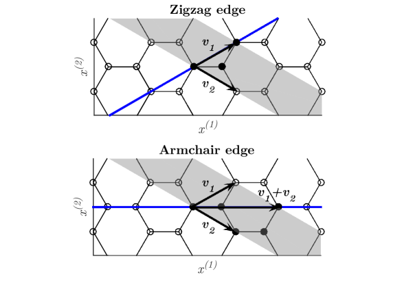
Figure 6. Bulk honeycomb structure, ${\bf H}=({\bf A}+\Lambda_{h})\cup({\bf B}+\Lambda_{h})$. Top panel: Zigzag edge, ${\bm{\mathfrak{v}}}_{1}={\bf v}_{1},{\bm{\mathfrak{K}}}_{2}={\bf k}_{2}$, $\mathbb{R}{\bf v}_{1}=\{{\bf x}:{\bf k}_{2}\cdot{\bf x}=0\}$ (blue line). Shaded region is the fundamental domain of cylinder, $\Sigma_{ZZ}$, corresponding to the zigzag edge. Bottom panel: Armchair edge, ${\bm{\mathfrak{v}}}_{1}={\bf v}_{1}+{\bf v}_{2},{\bm{\mathfrak{K}}}_{2}={\bf k}_{2}-{\bf k}_{1}$, $\mathbb{R}\left({\bf v}_{1}+{\bf v}_{2}\right)=\{{\bf x}:({\bf k}_{1}-{\bf k}_{2})\cdot{\bf x}=0\}$ (blue line). Fundamental domain of cylinder, $\Sigma_{AC}$, corresponding to the armchair edge.

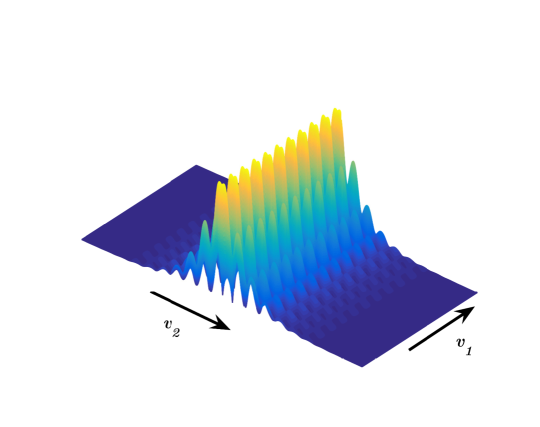
Figure 7. Edge state – propagating (plane-wave like) parallel to a zigzag edge ($\mathbb{R}{\bf v}_{1}$) and localized transverse to the edge

Introduce the family of Hamiltonians, depending on the real parameters $\lambda$ and $\delta$:

$$H^{(\lambda,\delta)}\equiv-\Delta+\lambda^{2}V({\bf x})+\delta\kappa(\delta{\bm{\mathfrak{K}}}_{2}\cdot{\bf x})W({\bf x}).$$

$H^{(\lambda,0)}=-\Delta+\lambda^{2}V({\bf x})$ is the Hamiltonian for the unperturbed (bulk) honeycomb structure, studied in Theorem 6.1. Here, $\delta$ will be taken to be sufficiently small, and $W({\bf x})$ is $\Lambda_{h}-$ periodic and odd with respect to the center, ${\bf x}_{c}$, i.e. $W(2{\bf x}_{c}-{\bf x})=-W({\bf x})$. Thus, $W$ breaks inversion symmetry. See Corollary 6.3. The function $\kappa(\zeta)$ defines a domain wall. We choose $\kappa$ to be sufficiently smooth and to satisfy $\kappa(0)=0$ and $\kappa(\zeta)\to\pm\kappa_{\infty}\neq 0$ as $\zeta\to\pm\infty$, e.g. $\kappa(\zeta)=\tanh(\zeta)$. Without loss of generality, we assume $\kappa_{\infty}>0$.

Note that $H^{(\lambda,\delta)}$ is invariant under translations parallel to the ${\bm{\mathfrak{v}}}_{1}-$ edge, ${\bf x}\mapsto{\bf x}+{\bm{\mathfrak{v}}}_{1}$, and hence there is a well-defined parallel quasi-momentum, denoted ${k_{\parallel}}$. Furthermore, $H^{(\lambda,\delta)}$ transitions adiabatically between the asymptotic Hamiltonian $H_{-}^{(\lambda,\delta)}=H^{(\lambda,0)}-\delta\kappa_{\infty}W({\bf x})$ as ${\bm{\mathfrak{K}}}_{2}\cdot{\bf x}\to-\infty$ to the asymptotic Hamiltonian $H_{+}^{(\lambda,\delta)}=H^{(\lambda,0)}+\delta\kappa_{\infty}W({\bf x})$ as ${\bm{\mathfrak{K}}}_{2}\cdot{\bf x}\to\infty$. The domain wall modulation of $W({\bf x})$ realizes a phase-defect across the edge $\mathbb{R}{\bm{\mathfrak{v}}}_{1}$. A variant of this construction was used in [FLW-PNAS:14, FLW-MAMS:17] to interpolate between different asymptotic 1D dimer periodic potentials.

We seek ${\bm{\mathfrak{v}}}_{1}-$ edge states of $H^{(\lambda,\delta)}$, which are spectrally localized near the Dirac point, $({\bf K}_{\star},E^{\lambda}_{D})$, where ${\bf K}_{\star}$ is a vertex of ${\mathcal{B}}_{h}$. These are non-trivial solutions $\Psi$, with energies $E\approx E^{\lambda}_{D}$, of the ${k_{\parallel}}-$ edge state eigenvalue problem (EVP):

(6.11) $$H^{(\lambda,\delta)}\Psi =E\Psi,$$

(6.12) $$\Psi({\bf x}+{\bm{\mathfrak{v}}}_{1}) =e^{i{k_{\parallel}}}\Psi({\bf x}),$$

(6.13) $$|\Psi({\bf x})|\to\ 0\ {\rm as}\ |{\bm{\mathfrak{K}}}_{2}\cdot{\bf x}|\to\infty,$$

for ${k_{\parallel}}\approx{\bf K}_{\star}\cdot{\bm{\mathfrak{v}}}_{1}$. The boundary conditions (6.12) and (6.13) imply, respectively, propagation parallel to, and localization transverse to, the edge $\mathbb{R}{\bm{\mathfrak{v}}}_{1}$.

The edge state eigenvalue problem (6.11)-(6.13) may be formulated in an appropriate Hilbert space. Introduce the cylinder $\Sigma\equiv\mathbb{R}^{2}/\mathbb{Z}{\bm{\mathfrak{v}}}_{1}$. Denote by $H^{s}(\Sigma),\ s\geq 0$, the Sobolev spaces of functions defined on $\Sigma$. The pseudo-periodicity and decay conditions (6.12)-(6.13) are encoded by requiring $\Psi\in H^{s}_{k_{\parallel}}(\Sigma)=H^{s}_{k_{\parallel}}$, for some $s\geq 0$, where

$$H^{s}_{k_{\parallel}}\equiv\ \left\{f:f({\bf x})e^{-i\frac{{k_{\parallel}}}{2\pi}{\bm{\mathfrak{K}}}_{1}\cdot{\bf x}}\in H^{s}(\Sigma)\right\}.$$

We then formulate the EVP (6.11)-(6.13) as:

(6.14) $$H^{(\lambda,\delta)}\Psi=E\Psi,\quad\Psi\in H^{2}_{{k_{\parallel}}}(\Sigma).$$

Theorem 7.3 and Corollary 7.4 in [FLW-2d_edge:16] (see also Theorem 4.1 of [FLW-2d_materials:15]) formulate general hypotheses on the bulk honeycomb structure, $V({\bf x})$, the domain-wall function, $\kappa(\zeta)$, and the asymptotic perturbation of the bulk structure, $W({\bf x})$, which imply the existence of topologically protected ${\bm{\mathfrak{v}}}_{1}-$ edge states, constructed as non-trivial eigenpairs $\delta\mapsto(\Psi^{\delta},E^{\delta})$ (6.14) with ${k_{\parallel}}={\bf K}_{\star}\cdot{\bm{\mathfrak{v}}}_{1}$, defined for all $|\delta|$ sufficiently small. This branch of solutions bifurcates, for $\delta\neq 0$, from the intersection of spectral bands at $E_{D}$.

The key hypothesis is a spectral no-fold condition, associated with ${\bm{\mathfrak{v}}}_{1}-$ edge. In [FLW-2d_edge:16], this condition was verified for the zigzag edge, for general honeycomb Schrödinger operators, $-\Delta+\varepsilon V$, with low contrast; in particular, where

$$\varepsilon V_{1,1}\ \equiv\ \varepsilon\ \int_{D}e^{-i({\bf k}_{1}+{\bf k}_{2})\cdot{\bf x}}V({\bf x})\ d{\bf x}>0,$$

with $|\varepsilon|$ sufficiently small.

The main result of the present article, Theorem 6.1, immediately implies the validity of the spectral no-fold condition for all $\lambda>\lambda_{\star}$ sufficiently large, and hence

Corollary 6.4 (Protected edge states for rational edges).

In the strong binding regime, there exist topologically protected edge states for the large class of rational edges presented in Remark 6.5 below.

The class of admissible edges in Corollary 6.4 is presented in Remark 6.5 below.

We next present a brief explanation of the spectral no-fold condition. Given an edge in the direction of ${\bm{\mathfrak{v}}}_{1}\in\Lambda_{h}$, there is an associated dual slice of the band structure, which passes through a chosen Dirac point, $({\bf K}_{\star},E_{D})$. The dual slice is the set of curves $\xi\in[-1/2,1/2)\mapsto E_{b}({\bf K}_{\star}+\xi{\bm{\mathfrak{K}}}_{2}),\ b\geq 1$, where ${\bm{\mathfrak{K}}}_{2}\cdot{\bm{\mathfrak{v}}}_{1}=0$. The significance of the dual slice is that the edge-states constructed in [FLW-2d_edge:16], which are propagating parallel to and localized transverse to ${\bm{\mathfrak{v}}}_{1}$, are superpositions of Floquet-Bloch modes with the quasi-momenta of the dual slice. In the current setting, we verify the spectral no-fold condition for the two lowest spectral bands of $-\Delta+\lambda^{2}V({\bf x})$ for $\lambda>\lambda_{\star}$ sufficiently large. The spectral no-fold condition states that the line $E=E_{D}$ intersects the pair of dispersion curves $\xi\in[-1/2,1/2)\mapsto E_{1}({\bf K}_{\star}+\xi{\bm{\mathfrak{K}}}_{2}),\ E_{2}({\bf K}_{\star}+\xi{\bm{\mathfrak{K}}}_{2})$, only at Dirac points.

Figure 8 illustrates such pairs of dispersion curves, associated with several edges: zigzag, armchair and $(2,1)$ and two choices of $\lambda$: $\lambda=1$ and $5$. For $\lambda=1$, the no-fold condition holds only for the zigzag edge, but it holds for all three types of edges if $\lambda=5$.

Remark 6.5.

1. At present, the results in [FLW-2d_edge:16] are stated for edges, $\mathbb{R}{\bm{\mathfrak{v}}}_{1}$, for which $\xi\mapsto{\bf K}_{\star}+\xi{\bm{\mathfrak{K}}}_{2}$, $|\xi|\leq 1/2$, passes through only one independent Dirac point. There are edges for which the dual slice passes through two independent Dirac points, i.e. where $\xi\mapsto{\bf K}_{\star}+\xi{\bm{\mathfrak{K}}}_{2}$, $|\xi|\leq 1/2$ intersects both lattices ${\bf K}_{\star}+\Lambda_{h}^{*}$ and ${\bf K}_{\star}^{\prime}+\Lambda_{h}^{*}$. We are currently working on extending the methods of [FLW-2d_edge:16] to this case. See [FLW-2d_materials:15] for a discussion and numerical simulations of the multi-branch bifurcation from the intersection of bands in this case.

2. Our results imply that given an edge in the direction ${\bm{\mathfrak{v}}}^{(m,n)}_{1}=m{\bf v}_{1}+n{\bf v}_{1}$, where $m$ and $n$ are relatively prime integers, there is a threshold $\lambda_{\star}(m,n)$, such that for all $\lambda>\lambda_{\star}(m,n)$, the spectral no-fold condition holds and there exist edge states [FLW-2d_materials:15].

3. As discussed above, in [FLW-2d_edge:16] we prove the existence of zigzag edge states (${\bm{\mathfrak{v}}}^{(m,n)}_{1}={\bm{\mathfrak{v}}}^{(1,0)}_{1}$) for a class of line-defect perturbations of Schrödinger operators with weak honeycomb potentials: $-\Delta+\varepsilon V_{h}({\bf x}),\ |\varepsilon|\ll 1$, satisfying the additional condition: $\varepsilon V_{1,1}>0$. This analysis also suggests that if $\varepsilon V_{1,1}<0$, then there are edge quasi-modes, whose energy slowly leaks into the bulk. By appropriate choice of atomic potential well $V_{0}({\bf x})$, we may arrange for $V({\bf x})$, such that $\varepsilon V_{1,1}<0$; see Appendix A of [FLW-2d_edge:16]. For honeycomb potentials, $V$, arising from such atomic potentials, Corollary 6.4 shows that there is necessarily a transition from a “leaky” resonance mode to a truly localized mode along the edge, for $\lambda$ above some finite $\lambda_{\star}$.

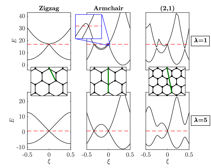
Figure 8. Band dispersion slices of $-\Delta+\lambda^{2}V$ along the quasi-momentum segments: ${\bf K}+\xi{\bm{\mathfrak{K}}}_{2},\ |\xi|\leq 1/2$, for ${\bm{\mathfrak{K}}}_{2}={\bf k}_{2}$ (zigzag), ${\bm{\mathfrak{K}}}_{2}=-{\bf k}_{1}+{\bf k}_{2}$ (armchair) and ${\bm{\mathfrak{K}}}_{2}=-{\bf k}_{1}+2{\bf k}_{2}$ ($(2,1)$), for $\lambda=1$ (top row) and $\lambda=5$ (bottom row). Numerical computations presented are for the simple trigonometric polynomial potential $V({\bf x})=\cos({\bf k}_{1}\cdot{\bf x})+\cos({\bf k}_{2}\cdot{\bf x})+\cos(({\bf k}_{1}+{\bf k}_{2})\cdot{\bf x})$, satisfying $V_{1,1}>0$, which is not of the form of the potentials introduced in Section 5. Red dashed lines denote the Dirac point energy, $E^{\lambda}_{D}$. Top row: $\lambda=1$. Spectral no-fold condition holds for the zigzag edge but not the armchair and $(2,1)-$ edge. Bottom row: $\lambda=5$. Spectral no-fold condition holds for all three edges. Insets between dispersion slice plots indicate zigzag, armchair and $(2,1)-$ (green) quasi-momentum segments (1D Brillouin zones) parametrized by $\xi$, for $0\leq\xi\leq 1$.

7. Dirac points

In this section we summarize results of [FW:12] on Dirac points of Schrödinger Hamiltonians, $H_{V}=-\Delta+V$, where $V$ is a honeycomb lattice potential. In the current context our Hamiltonian is $H^{\lambda}=-\Delta+\lambda^{2}V({\bf x})-E_{0}^{\lambda}$, with $V$ defined in (5.1).

Introduce the rotation and inversion operators, acting on functions:

(7.1) $$\mathcal{R}[f]({\bf x})=f({\bf x}_{c}+R^{*}({\bf x}-{\bf x}_{c}))\ {\rm and}\ \mathcal{I}[f]({\bf x})=f({\bf x}_{c}-({\bf x}-{\bf x}_{c}))=f(2{\bf x}_{c}-{\bf x}).$$

Let ${\bf K}_{\star}$ denote any vertex of the Brillouin zone, $\mathcal{B}_{h}$, and let $f$ be a ${\bf K}_{\star}-$ pseudo-periodic function. Since $R^{*}$ maps $\Lambda_{h}$ to itself and $R{\bf K}_{\star}\in{\bf K}_{\star}+\Lambda_{h}^{*}$, we have

(7.2) $$\mathcal{R}[f]({\bf x}+{\bf v}) =f({\bf x}_{c}+R^{*}({\bf x}-{\bf x}_{c})+R^{*}{\bf v})=e^{i{\bf K}_{\star}\cdot R^{*}{\bf v}}f({\bf x}_{c}+R^{*}({\bf x}-{\bf x}_{c}))$$

$$=e^{iR{\bf K}_{\star}\cdot{\bf v}}f({\bf x}_{c}+R^{*}(x-{\bf x}_{c}))=e^{i{\bf K}_{\star}\cdot{\bf v}}f({\bf x}_{c}+R^{*}({\bf x}-{\bf x}_{c}))$$

$$=e^{i{\bf K}_{\star}\cdot{\bf v}}\ \mathcal{R}[f]({\bf x}).$$

Therefore, in analogy with Proposition 2.2 of [FW:12] we have

Proposition 7.1.

Let ${\bf K}_{\star}$ be any of the six vertices of the Brillouin zone, ${\mathcal{B}}_{h}$. Then, $H^{\lambda}$ and $\mathcal{R}$ map a dense subspace of $L^{2}_{{\bf K}_{\star}}$ to itself. Furthermore, restricted to this dense subspace, the commutator $[H^{\lambda},\mathcal{R}]=H^{\lambda}\ \mathcal{R}-\mathcal{R}\ H^{\lambda}$ vanishes. In particular, if $\phi({\bf x},{\bf K}_{\star})$ is a solution of the ${\bf K}_{\star}-$ pseudo-periodic eigenvalue problem (5.5), then $\mathcal{R}[\phi(\cdot,{\bf K}_{\star})]({\bf x})$ is also a solution of (5.5).

Since $\mathcal{R}$ has eigenvalues $1,\tau$ and $\overline{\tau}$, it is natural to split $L^{2}_{{\bf K}_{\star}}$, the space of ${\bf K}_{\star}-$ pseudo-periodic functions, into the direct sum:

(7.3) $$L^{2}_{{\bf K}_{\star}}\ =\ L^{2}_{{\bf K}_{\star},1}\oplus L^{2}_{{\bf K}_{\star},\tau}\oplus L^{2}_{{\bf K}_{\star},\overline{\tau}}.$$

Here, $L^{2}_{{\bf K}_{\star},\sigma}$, where $\sigma=1,\tau,\overline{\tau}$ and $\tau=\exp(2\pi i/3)$, denote the invariant eigenspaces of $\mathcal{R}$:

(7.4) $$L^{2}_{{\bf K}_{\star},\sigma}\ =\ \Big{\{}g\in L^{2}_{{\bf K}_{\star}}:\mathcal{R}g=\sigma g\Big{\}}\ .$$

We also introduce $H^{s}_{{\bf K}_{\star}}$, $s\geq 0$, the subspace of functions $f\in L^{2}_{{\bf K}_{\star}}$, such that $e^{-i{\bf K}_{\star}\cdot{\bf x}}f({\bf x})\in H^{2}(\mathbb{R}^{2}/\Lambda_{h})$. $H^{s}_{{\bf K}_{\star},\sigma}$, for $s\geq 0$ and $\sigma=1,\tau,\overline{\tau}$, a subspace of $L^{2}_{{\bf K}_{\star},\sigma}$ is defined analogously.

Proposition 7.1 and the decomposition (7.3) imply that the $L^{2}_{{\bf K}_{\star}}-$ Floquet-Bloch eigenvalue problem may be reduced to the three independent $L^{2}_{{\bf K}_{\star},\sigma}-$ eigenvalue problems;

$$\left(-\Delta+\lambda^{2}V\right)\Psi\ =\ E\Psi,\qquad\Psi\in L^{2}_{{\bf K}_{\star},\sigma}\qquad\sigma=1,\tau,\overline{\tau};$$

In particular, see Definition 7.3 of Dirac point below.

Proposition 7.2.

Let $f\in L^{2}_{{\bf K}_{\star},\tau}$. Then,

$$\left(\mathcal{C}\circ\mathcal{I}\right)[f]({\bf x})\equiv\overline{f(2{\bf x}_{c}-{\bf x})}\ \in\ L^{2}_{{\bf K}_{\star},\overline{\tau}},\$$

where $\mathcal{C}$ denotes complex-conjugation and $\mathcal{I}$ is the inversion with respect to ${\bf x}_{c}$, defined in (7.1).

Proof of Proposition 7.2.

Let $S=\mathcal{C}\circ\mathcal{I}$ and suppose $f\in L^{2}_{{\bf K}_{\star},\tau}$. Then, for any ${\bf v}\in\Lambda_{h}$,

$$[Sf]({\bf x}+{\bf v})=\overline{f(2{\bf x}_{c}-{\bf x}-{\bf v})}=\overline{f(2{\bf x}_{c}-{\bf x})e^{i{\bf K}_{\star}\cdot(-{\bf v})}}=e^{i{\bf K}_{\star}\cdot{\bf v}}[Sf]({\bf x}).$$

Hence, $Sf\in L^{2}_{{\bf K}_{\star}}$. Furthermore,

$$\mathcal{R}[Sf]({\bf x}) =\ (Sf)\left({\bf x}_{c}+R^{*}({\bf x}-{\bf x}_{c})\right)\ =\ \overline{f\left(2{\bf x}_{c}-[{\bf x}_{c}+R^{*}({\bf x}-{\bf x}_{c})]\right)}$$

$$=\ \overline{f\left({\bf x}_{c}+R^{*}[2{\bf x}_{c}-{\bf x}-{\bf x}_{c}])]\right)}=\overline{\tau\ f(2{\bf x}_{c}-{\bf x})}\ =\ \overline{\tau}\ S[f]({\bf x})\$$

which completes the proof.∎

We next give a precise definition of a Dirac point of a honeycomb Schroedinger operator; see [FW:12].

Definition 7.3 (Dirac point).

Let $V({\bf x})$ be smooth, real-valued and $\Lambda_{h}-$ periodic on $\mathbb{R}^{2}$. Assume, in addition that $V$ is inversion symmetric with respect to ${\bf x}_{c}$ and rotationally invariant by $120^{\circ}$; see (5.3). That is, $V$ is a honeycomb lattice potential in the sense of [FW:12]. Consider the Schrödinger operator $H_{V}=-\Delta+V$.

Denote by ${\mathcal{B}}_{h}$, the Brillouin zone. Let ${\bf K}_{\star}\in{\mathcal{B}}_{h}$ be one of the vertices of the Brillouin zone. The energy / quasi-momentum pair $({\bf K}_{\star},E_{D})\in{\mathcal{B}}_{h}\times\mathbb{R}$ is called a Dirac point if there exists $b_{\star}\geq 1$ such that:

1. $E_{D}$ is an $L^{2}_{{\bf K}_{\star}}-$ eigenvalue of $H_{V}$ of multiplicity two.

2. The eigenspace for the eigenvalue $E_{D}$, $\textrm{Nullspace}\Big{(}H_{V}-E_{D}I\Big{)}$, is equal to ${\rm span}\Big{\{}\Phi_{1},\Phi_{2}\Big{\}}$, where $\Phi_{1}\in L^{2}_{{\bf K}_{\star},\tau}$ is a solution of the $L^{2}_{{\bf K}_{\star},\tau}-$ Floquet-Bloch eigenvalue problem and $\Phi_{2}({\bf x})=\left(\mathcal{C}\circ\mathcal{I}\right)[\Phi_{1}]({\bf x})=\overline{\Phi_{1}(2{\bf x}_{c}-{\bf x})}\in L^{2}_{{\bf K}_{\star},\bar{\tau}}$ is a solution of the $L^{2}_{{\bf K}_{\star},\overline{\tau}}-$ Floquet-Bloch eigenvalue problem. We may take $\left\langle\Phi_{a},\Phi_{b}\right\rangle_{L^{2}_{{\bf K}_{\star}}}=\delta_{ab}$, $a,b=1,2$.

3. There exist constants ${v_{{}_{F}}}\in\mathbb{C}$, ${v_{{}_{F}}}\neq 0$ and $\zeta_{0}>0$, Floquet-Bloch eigenpairs

   $${\bf k}\mapsto(\Phi_{b_{\star}+1}({\bf x};{\bf k}),E_{b_{\star}+1}({\bf k}))\ \ {\rm and}\ \ {\bf k}\mapsto(\Phi_{b_{\star}}({\bf x};{\bf k}),E_{b_{\star}}({\bf k})),$$

   and Lipschitz continuous functions $e_{j}({\bf k}),\ j=b_{\star},b_{\star}+1$, where $e_{j}({\bf K}_{\star})=0$, defined for $|{\bf k}-{\bf K}_{\star}|<\zeta_{0}$ such that

   $$E_{b_{\star}+1}({\bf k})-E_{D}\ =\ +|{v_{{}_{F}}}|\ \left|{\bf k}-{\bf K}_{\star}\right|\ \left(1\ +\ e_{b_{\star}+1}({\bf k})\right),$$

   $$E_{b_{\star}}({\bf k})-E_{D}\ =\ -|{v_{{}_{F}}}|\ \left|{\bf k}-{\bf K}_{\star}\right|\ \left(1\ +\ e_{b_{\star}}({\bf k})\right).$$

   In particular, $|e_{j}({\bf k})|\lesssim|{\bf k}-{\bf K}_{\star}|,\ j=b_{\star},b_{\star}+1$.
   

Remark 7.4.

1. The quantity $|{v_{{}_{F}}}|$ is known as the Fermi velocity; see, for example, [RMP-Graphene:09].

2. In [FW:12] we prove that parts (1) and (2) of Definition 7.3 imply part (3), although ${v_{{}_{F}}}$ may be zero. We then show that for generic honeycomb lattice potentials, ${v_{{}_{F}}}\neq 0$. No assumptions are made on the size (contrast/depth) of the potential.

3. Note, from Proposition 4.1 of [FW:12] that ${v_{{}_{F}}}$ is given in terms of the Floquet-Bloch modes $\Phi_{1}$ and $\Phi_{2}$ by the expression:

   (7.5) $${v_{{}_{F}}}\ =\ 2\left\langle\Phi_{2},\frac{1}{i}\partial_{x_{1}}\Phi_{1}\right\rangle$$

4. Suppose $({\bf K},E_{D})$ is a Dirac point with corresponding eigenspace ${\rm span}\{\Phi_{1},\Phi_{2}\}$, where $\Phi_{1}\in L^{2}_{{\bf K},\tau}$ and $\Phi_{2}\in L^{2}_{{\bf K},\bar{\tau}}$. Then, since $\mathcal{R}$ commutes with $-\Delta+\lambda^{2}V$, and since the quasi-momenta $R{\bf K}$ and $R^{2}{\bf K}$ yield equivalent pseudo-periodicity to ${\bf K}$ we have that $({\bf K},E_{D})$, $(R{\bf K},E_{D})$ and $(R^{2}{\bf K},E_{D})$ are all Dirac points. Moreover, since $V$ is real-valued, complex-conjugation yields that $({\bf K}^{\prime},E_{D})$, $(R{\bf K}^{\prime},E_{D})$ and $(R^{2}{\bf K}^{\prime},E_{D})$ are all Dirac points. So to establish that there are Dirac points located at the six vertices of ${\mathcal{B}}_{h}$, it suffices to prove this for a single vertex of ${\mathcal{B}}_{h}$.

8. Approximation of low-lying Floquet-Bloch modes for large $\lambda$

In this section and in Section 9 we assume that ${\rm supp}(V_{0})\subset B({\bf 0},r_{0})$, where $0<r_{0}<\frac{1}{2}|{\bf e}_{A,1}|\times(1-\delta_{0})$, for some small given $\delta_{0}>0$. The stricter constraint $(PW_{2})$ on the size of ${\rm supp}(V_{0})$ in the statement of Theorem 6.1 is used in the analysis starting in Section 10.

Starting with the ground state eigenfunction, $p_{0}^{\lambda}({\bf x})$, we define

$$p_{\bf k}^{\lambda}({\bf x})\ =\ e^{-i{\bf k}\cdot{\bf x}}\ p_{0}^{\lambda}({\bf x}),\qquad{\bf k}\in\mathbb{C}^{2},\ \ {\bf x}\in\mathbb{R}^{2}.$$

For now, assume $|\Im{\bf k}|<C_{1}$, where $C_{1}$ is a fixed positive number. (We shall later further constrain ${\bf k}$ by $|\Im{\bf k}|\leq\lambda^{-1}$. ) Since $p_{0}^{\lambda}({\bf x})$ satisfies the exponential decay bound (see Corollary 15.5) $p_{0}^{\lambda}({\bf x})\lesssim e^{-c\lambda|{\bf x}|},\ |{\bf x}|>R_{0}$, for $\lambda$ larger than some constant depending on $C_{1}$, $p_{\bf k}^{\lambda}({\bf x})$ is also exponentially decaying.

For fixed ${\bf k}\in\mathbb{R}^{2}$ we have

$$\left[\ -\left(\ \nabla_{\bf x}+i{\bf k}\right)^{2}\ +\ \lambda^{2}V_{0}({\bf x})\ -\ E_{0}^{\lambda}\ \right]p_{\bf k}^{\lambda}({\bf x})=0$$

and

(8.1) $$\left\langle\ \left(\ -\left(\ \nabla_{\bf x}+i{\bf k}\right)^{2}+\lambda^{2}V_{0}\ \right)\psi,\psi\ \right\rangle_{{}_{L^{2}(\mathbb{R}^{2})}}\ \geq\ (E_{0}^{\lambda}+c_{gap})\ \|\psi\|_{{}_{L^{2}(\mathbb{R}^{2})}}^{2},$$

for $\psi\in H^{2}(\mathbb{R}^{2})$ such that $\left\langle p_{\bf k}^{\lambda},\psi\right\rangle_{{}_{L^{2}(\mathbb{R}^{2})}}=0$, by property (EG) in Section 4.

Introduce the recentering of $p_{\bf k}^{\lambda}$ at $\hat{\bf v}\in{\bf H}=\Lambda_{A}\cup\Lambda_{B}$:

$$p_{{\bf k},\hat{\bf v}}^{\lambda}({\bf x})\ \equiv\ p_{\bf k}^{\lambda}({\bf x}-\hat{\bf v})\ ,$$

and define the $\Lambda_{h}-$ periodic approximate Floquet-Bloch amplitudes:

(8.2) $$p_{{\bf k},I}^{\lambda}({\bf x})\ \equiv\ \sum_{\hat{\bf v}\in\Lambda_{I}}\ p_{{\bf k},\hat{\bf v}}^{\lambda}({\bf x})\ =\ \sum_{\hat{\bf v}\in\Lambda_{I}}\ e^{-i{\bf k}\cdot({\bf x}-\hat{\bf v})}p_{0}^{\lambda}({\bf x}-\hat{\bf v})\ ,\ I=A,B.$$

and the ${\bf k}-$ pseudo-periodic approximate Floquet-Bloch modes:

(8.3) $$P_{{\bf k},A}^{\lambda}({\bf x})\equiv e^{i{\bf k}\cdot{\bf x}}\ p_{{\bf k},A}^{\lambda}({\bf x}),\qquad P_{{\bf k},B}^{\lambda}({\bf x})\equiv e^{i{\bf k}\cdot{\bf x}}\ p_{{\bf k},B}^{\lambda}({\bf x})\ .$$

Remark 8.1.

In Theorem 10.1 we construct eigenstates of $-\Delta+\lambda^{2}V$, $\lambda$ large: $\Phi_{1}^{\lambda}({\bf x})$ near $P_{{\bf K},A}^{\lambda}({\bf x})\equiv e^{i{\bf K}\cdot{\bf x}}\ p_{{\bf K},A}^{\lambda}({\bf x})\in L^{2}_{{\bf K},\tau}$ and $\Phi_{2}^{\lambda}({\bf x})$ near $P_{{\bf K},B}^{\lambda}({\bf x})\equiv e^{i{\bf K}\cdot{\bf x}}\ p_{{\bf K},B}^{\lambda}({\bf x})\in L^{2}_{{\bf K},\overline{\tau}}$.

We find it useful to let the mapping ${\bf k}\mapsto p_{{\bf k},I}^{\lambda}$ depend on a complex quasi-momentum, ${\bf k}$, varying in an appropriate domain in $\mathbb{C}^{2}$. Corollary 15.5, to be proved later, shows that $p_{0}^{\lambda}({\bf x})$ satisfies the exponential decay bound $p_{0}^{\lambda}({\bf x})\lesssim e^{-c\lambda|{\bf x}|},\ |{\bf x}|>r_{0}+c_{0}$. The function $p_{{\bf k},I}^{\lambda}({\bf x})$ is $\Lambda_{h}-$ periodic on $\mathbb{R}^{2}$ so it may be regarded as a function on $\mathbb{R}^{2}/\Lambda_{h}$.

Furthermore, by the exponential decay of $p_{{\bf k}}^{\lambda}({\bf x})$, for all $\lambda$ larger than a constant which depends on $C_{1}$, the series (8.2) converges uniformly to an analytic function:

$${\bf k}\mapsto p_{{\bf k},I}^{\lambda} \{{\bf k}\in\mathbb{C}^{2}:|\Im{\bf k}|<C_{1}\} H^{2}(\mathbb{R}^{2}/\Lambda_{h})$$ from to .

This property is used in Section 14.2, where we obtain derivative bounds on the rescaled dispersion maps near Dirac points via Cauchy estimates for quasi-momenta, ${\bf k}$, in a narrow strip, $\{{\bf k}\in\mathbb{C}^{2}\ :\ |\Im{\bf k}|<\hat{c}\lambda^{-1}\}$, where $\hat{c}$ is a small constant.

We state further consequences of exponential decay of $p_{0}^{\lambda}$. For $|\Im{\bf k}|<C_{1}$,

(8.4) $$\Big{|}\ \|p_{{\bf k},I}^{\lambda}\|_{{}_{L^{2}(\mathbb{R}^{2}/\Lambda_{h})}}\ -\ 1\ \Big{|}\ \lesssim\ e^{-c\lambda},\ I=A,B.$$

(8.5) $$\Big{|}\ \left\langle p^{\lambda}_{{\bf k},J},p^{\lambda}_{{\bf k},I}\right\rangle_{{}_{L^{2}(\mathbb{R}^{2}/\Lambda_{h})}}\ -\ \delta_{JI}\ \Big{|}\ \lesssim\ e^{-c\lambda},\ I=A,B,\quad\text{and}$$

(8.6) $$\|\ p_{{\bf k},I}^{\lambda}-p_{{\bf k},{\bf v}}^{\lambda}\ \|_{{}_{L^{2}(\mathscr{Z}_{\bf v})}}\ \lesssim\ e^{-c\lambda},\ {\bf v}\in\Lambda_{I},\ \ I=A,B.$$

Here, $\mathscr{Z}_{\bf v}$, for ${\bf v}\in\Lambda_{I}$, is the set of points in $\mathbb{R}^{2}$ which are at least as close to ${\bf v}$ as to any other point in $\Lambda_{I}$.

For $|\Im{\bf k}|<C_{1}$, we claim that:

(8.7) $$\|H^{\lambda}({\bf k})p_{{\bf k},I}^{\lambda}\|\equiv\|\left[-(\nabla_{\bf x}+i{\bf k})^{2}+V^{\lambda}({\bf x})\right]p_{{\bf k},I}^{\lambda}\|_{{}_{L^{2}(\mathbb{R}^{2}/\Lambda_{h})}}\lesssim e^{-c\lambda},\ I=A,B.$$

Here, $V^{\lambda}({\bf x})=\lambda^{2}V({\bf x})-E_{D}^{\lambda}=\lambda^{2}\sum_{{\bf v}\in{\bf H}}\ V_{0}({\bf x}-{\bf v})-E_{D}^{\lambda}$; see (5.4). The bound (8.7) follows from exponential decay of $p_{\bf k}^{\lambda}$, a consequence of Corollary 15.5 (exponential decay of $p_{0}^{\lambda}({\bf x})$), and the observation

$$H^{\lambda}({\bf k})p_{{\bf k},\hat{\bf v}}^{\lambda}({\bf x}) \equiv\left[-(\nabla_{\bf x}+i{\bf k})^{2}+V^{\lambda}({\bf x})\right]p_{{\bf k},\hat{\bf v}}^{\lambda}({\bf x})$$

$$=\left[-(\nabla_{\bf x}+i{\bf k})^{2}+\lambda^{2}V_{0}({\bf x}-\hat{\bf v})-E_{0}^{\lambda}+\sum_{{\bf v}\in{\bf H}\setminus\{\hat{\bf v}\}}\lambda^{2}V_{0}({\bf x}-{\bf v})\right]p_{{\bf k}}^{\lambda}({\bf x}-\hat{\bf v})$$

(8.8) $$=\sum_{{\bf v}\in{\bf H}\setminus\{\hat{\bf v}\}}\lambda^{2}V_{0}({\bf x}-{\bf v})p_{{\bf k}}^{\lambda}({\bf x}-\hat{\bf v}).$$

Let ${\tilde{\bf K}}\in\mathbb{R}^{2}$ denote a generic real quasi-momentum and assume $|{\bf k}-{\tilde{\bf K}}|\lesssim\lambda^{-1}$. Then, using the exponential decay of $p_{0}^{\lambda}$, we obtain

(8.9) $$\left\|\ p_{{\bf k},I}^{\lambda}-p_{{\tilde{\bf K}},I}^{\lambda}\ \right\|\ \lesssim\ \lambda^{-1}\ .$$

The following lemma facilitates our working with a nearly orthogonal decomposition of $L^{2}(\mathbb{R}^{2}/\Lambda_{h})$ in terms of ${\rm span}\left\{p_{{\bf k},I}^{\lambda}:I=A,B\right\}$ and ${\rm span}\left\{p_{{\tilde{\bf K}},I}^{\lambda}:I=A,B\right\}^{\perp}$ provided the difference $|{\bf k}-{\tilde{\bf K}}|$ is sufficiently small.

Lemma 8.2.

Introduce the orthogonal projection

$$\Pi_{{}_{AB}}:L^{2}(\mathbb{R}^{2}/\Lambda_{h})\to\mathscr{H}_{{}_{AB}}\ \ {\rm onto}$$

$$\mathscr{H}_{{}_{AB}}\ =\ \left\{\tilde{\psi}\in L^{2}(\mathbb{R}^{2}/\Lambda_{h})\ :\ \left\langle p_{{\tilde{\bf K}},I}^{\lambda},\tilde{\psi}\right\rangle=0,\ {\rm for}\ I=A,B\right\},$$

the orthogonal complement of ${\rm span}\left\{p_{{\tilde{\bf K}},I}^{\lambda}\ :\ I=A,B\ \right\}$ in $L^{2}(\mathbb{R}^{2}/\Lambda_{h})$.
Assume ${\tilde{\bf K}}\in\mathbb{R}^{2}$ and $|{\bf k}-{\tilde{\bf K}}|\lesssim\lambda^{-1}$.

1. Then, for $F\in L^{2}(\mathbb{R}^{2}/\Lambda_{h})$, we have that

   $$F=0\ \ \iff\ \ \Pi_{{}_{AB}}F=0\ \ {\rm and}\ \ \left\langle p_{{}_{\overline{k},I}}^{\lambda},F\right\rangle=0,\ \ I=A,B.$$

2. Any $\psi\in H^{2}(\mathbb{R}^{2}/\Lambda_{h})$ may be expressed in the form

   (8.10) $$\psi\ =\ \sum_{I=A,B}\ \alpha_{I}\ p_{{\bf k},I}^{\lambda}\ +\ \tilde{\psi},$$

   where $\tilde{\psi}\in\mathscr{H}_{{}_{AB}}^{2}$ and $\alpha_{A},\alpha_{B}\in\mathbb{C}$.

Proof of Lemma 8.2.

To prove part (1), assume $\Pi_{{}_{AB}}F=0$ and $\left\langle p_{{}_{\overline{k},I}}^{\lambda},F\right\rangle=0,\ \ I=A,B$. Then, $F=\sum_{I=A,B}\alpha_{{}_{I}}p_{{}_{{\tilde{\bf K}},I}}^{\lambda}$. Taking the inner product with $p_{{}_{\overline{k},A}}^{\lambda}$ and $p_{{}_{\overline{k},B}}^{\lambda}$ yields the equations

$$\sum_{I=A,B}\ \left\langle p_{{}_{\overline{k},J}}^{\lambda},p_{{}_{{\tilde{\bf K}},I}}^{\lambda}\right\rangle\alpha_{I}\ =\ 0,\quad\text{for\ \ }J=A,B.$$

The latter may be rewritten as

(8.11) $$\sum_{I=A,B}\ \Big{[}\ \left\langle p_{{}_{{\tilde{\bf K}},J}}^{\lambda},p_{{}_{{\tilde{\bf K}},I}}^{\lambda}\right\rangle+\left\langle\left[p_{{}_{\overline{k},J}}^{\lambda}-p_{{}_{{\tilde{\bf K}},J}}^{\lambda}\right],p_{{}_{{\tilde{\bf K}},I}}^{\lambda}\right\rangle\ \Big{]}\ \alpha_{I}\ =\ 0,\ J=A,B\ .$$

By (8.5), the first inner product within the square brackets is equal to $\delta_{JI}+\mathcal{O}(e^{-c\lambda})$ and by (8.9), the second inner product is $\mathcal{O}(\lambda^{-1})$. It follows that $\alpha_{I}=0,\ I=A,B$. Hence, $F=0$.

To prove part (2), note that (8.10) holds if and only if

$$\left\langle p^{\lambda}_{{\tilde{\bf K}},J},\psi\right\rangle\ =\ \sum_{I=A,B}\left\langle p^{\lambda}_{{\tilde{\bf K}},J},p^{\lambda}_{{\bf k},I}\right\rangle\ \alpha_{I}\ \ {\rm for}\ \ J=A,B.$$

By (8.5), $\left\langle p^{\lambda}_{{\tilde{\bf K}},J},p^{\lambda}_{{\bf K},I}\right\rangle\ \alpha_{I}=\delta_{J,I}+\mathcal{O}(e^{-c\lambda})$, and we may solve for $\alpha_{A}$ and $\alpha_{B}$ for $\lambda$ sufficiently large. This completes the proof of Lemma 8.2. ∎

9. Energy estimates

Throughout this section, we follow the convention (see Section 1.5) that in relations involving norms and inner products for which the relevant function space is not explicitly indicated, it is to be understood that these are taken in $L^{2}(\mathbb{R}^{2}/\Lambda_{h})$.

The following result is the point of departure for our energy estimates and resolvent bounds.

Lemma 9.1.

Fix $I=A$ or $B$. Assume that ${\rm supp}(V_{0})\subset B({\bf 0},r_{0})$, where $0<r_{0}<\frac{1}{2}|{\bf e}_{A,1}|\times(1-\delta_{0})$ for $\delta_{0}>0$ and fixed.

Suppose $\psi\in H^{2}(\mathbb{R}^{2}/\Lambda_{h})$ and ${\bf k}\in\mathbb{R}^{2}$. Assume that $\textrm{supp}\ \psi\subset\{{\bf x}\in\mathbb{R}^{2}/\Lambda_{h}:{\rm dist}({\bf x},\Lambda_{I})\leq r_{0}\}$ and that

$$\left\langle p_{{\bf k},I}^{\lambda},\psi\right\rangle_{L^{2}(\mathbb{R}^{2}/\Lambda_{h})}\ =\ 0.$$

Then,

$$\left\langle\left[-(\nabla_{\bf x}+i{\bf k})^{2}+V^{\lambda}({\bf x})\right]\psi,\psi\right\rangle_{L^{2}(\mathbb{R}^{2}/\Lambda_{h})}\geq c\|\psi\|_{L^{2}(\mathbb{R}^{2}/\Lambda_{h})}^{2}\ .$$

Proof of Lemma 9.1.

Fix $I=A$ or $B$ and let $\psi^{\sharp}({\bf x})=\psi({\bf x})\ {\bf 1}_{\{|{\bf x}-{\bf v}_{I}|\leq r_{0}\}}$ . Then,

$$\psi^{\sharp}\in H^{2}(\mathbb{R}^{2}),\ \ \textrm{supp}\ \psi^{\sharp}\subset\{{\bf x}\in\mathbb{R}^{2}:|{\bf x}-{\bf v}_{I}|\leq r_{0}\},$$

$$\psi({\bf x})=\sum_{{\bf v}\in\Lambda_{h}}\psi^{\sharp}({\bf x}-{\bf v}),$$

since the discs $\{{\bf x}\in\mathbb{R}^{2}:|{\bf x}-{\bf v}|<r_{0}\}$, where ${\bf v}\in\Lambda_{I}$, are disjoint subsets of $\mathbb{R}^{2}$; see Figure 4. Using the $\Lambda_{h}-$ periodicity of $V^{\lambda}({\bf x})$ we have:

$$\left\langle\left[-(\nabla_{\bf x}+i{\bf k})^{2}+V^{\lambda}({\bf x})\right]\psi,\psi\right\rangle_{L^{2}(\mathbb{R}^{2}/\Lambda_{h})}=\left\langle\left[-(\nabla_{\bf x}+i{\bf k})^{2}+V^{\lambda}({\bf x})\right]\psi^{\sharp},\psi^{\sharp}\right\rangle_{L^{2}(\mathbb{R}^{2})}.$$

We shall make use of the following consequence of (8.1):
Let $\eta\in H^{2}(\mathbb{R}^{2})$ satisfy $\left\langle p_{{\bf k},{\bf v}_{I}}^{\lambda},\eta\right\rangle_{L^{2}(\mathbb{R}^{2})}=0$. Then,

(9.1) $$\left\langle\ \left(\ -\left(\ \nabla_{\bf x}+i{\bf k}\right)^{2}+\lambda^{2}V_{0}({\bf x}-{\bf v}_{I})\ -E_{0}^{\lambda}\ \right)\eta,\eta\ \right\rangle_{L^{2}(\mathbb{R}^{2})}\ \geq\ c_{gap}\ \|\eta\|_{L^{2}(\mathbb{R}^{2})}^{2}\ .$$

Recall that by hypothesis on $\psi$ and the $\Lambda_{h}-$ periodicity of $p_{{\bf k},I}^{\lambda}$:

$$\left\langle p_{{\bf k},I}^{\lambda},\psi^{\sharp}\right\rangle_{L^{2}(\mathbb{R}^{2})}\ =\ \left\langle p_{{\bf k},I}^{\lambda},\psi\right\rangle_{L^{2}(\mathbb{R}^{2}/\Lambda_{h})}\ =0.$$

So to make use of (9.1), we should compare $\left\langle p_{{\bf k},{\bf v}_{I}}^{\lambda},\psi^{\sharp}\right\rangle_{L^{2}(\mathbb{R}^{2})}$ with $\left\langle p_{{\bf k},I}^{\lambda},\psi^{\sharp}\right\rangle_{L^{2}(\mathbb{R}^{2})}$.

By (8.6) and the Cauchy-Schwarz inequality

$$\Big{|}\ \left\langle p_{{\bf k},{\bf v}_{I}}^{\lambda},\psi^{\sharp}\right\rangle_{L^{2}(\mathbb{R}^{2})}\ -\ \left\langle p_{{\bf k},I}^{\lambda},\psi^{\sharp}\right\rangle_{L^{2}(\mathbb{R}^{2})}\ \Big{|}\ \lesssim\ e^{-c\lambda}\ \|\psi^{\sharp}\|_{L^{2}(\mathbb{R}^{2})}.$$

Hence,

(9.2) $$\Big{|}\left\langle p_{{\bf k},{\bf v}_{I}}^{\lambda},\psi^{\sharp}\right\rangle_{L^{2}(\mathbb{R}^{2})}\Big{|}\lesssim e^{-c\lambda}\ \|\psi^{\sharp}\|_{L^{2}(\mathbb{R}^{2})}.$$

Recall that $\|p^{\lambda}_{{\bf k},{\bf v}_{I}}\|_{L^{2}(\mathbb{R}^{2})}=\|p_{0}^{\lambda}\|_{L^{2}(\mathbb{R}^{2})}=1$. We may write

(9.3) $$\psi^{\sharp}=\alpha\ p^{\lambda}_{{\bf k},{\bf v}_{I}}+\psi^{\sharp\sharp},\ \ \left\langle p^{\lambda}_{{\bf k},{\bf v}_{I}},\psi^{\sharp\sharp}\right\rangle_{{}_{L^{2}(\mathbb{R}^{2})}}=0\ ,$$

where $\psi^{\sharp\sharp}\in H^{2}(\mathbb{R}^{2})$ and $\alpha\in\mathbb{C}$ . From (9.2) we have $|\alpha|\leq e^{-c\lambda}\ \|\psi^{\sharp}\|_{L^{2}(\mathbb{R}^{2})}$ and therefore

(9.4) $$\|\psi^{\sharp\sharp}\|_{L^{2}(\mathbb{R}^{2})}\geq(1-e^{-c\lambda})\|\psi^{\sharp}\|_{L^{2}(\mathbb{R}^{2})}\ .$$

Since $\left\langle p^{\lambda}_{{\bf k},{\bf v}_{I}},\psi^{\sharp\sharp}\right\rangle_{{}_{L^{2}(\mathbb{R}^{2})}}=0$, (9.1) and (9.4) imply

$$\left\langle\left[-(\nabla_{\bf x}+i{\bf k})^{2}+\lambda^{2}V_{0}({\bf x}-{\bf v}_{I})-E_{0}^{\lambda}\right]\psi^{\sharp\sharp},\psi^{\sharp\sharp}\right\rangle_{L^{2}(\mathbb{R}^{2})}$$

$$\qquad\qquad\geq\ c_{gap}\|\psi^{\sharp\sharp}\|_{L^{2}(\mathbb{R}^{2})}^{2}\ \geq\frac{1}{2}c_{gap}\ \|\psi^{\sharp}\|^{2}_{L^{2}(\mathbb{R}^{2})}\ .$$

However using (9.3) and the fact that $\left[-(\nabla_{\bf x}+i{\bf k})^{2}+\lambda^{2}V_{0}({\bf x}-{\bf v}_{I})-E_{0}^{\lambda}\right]p_{{\bf k},{\bf v}_{I}}^{\lambda}=0$ we have

$$\left\langle\left[-(\nabla_{\bf x}+i{\bf k})^{2}+\lambda^{2}V_{0}({\bf x}-{\bf v}_{I})-E_{0}^{\lambda}\right]\psi^{\sharp\sharp},\psi^{\sharp\sharp}\right\rangle_{L^{2}(\mathbb{R}^{2})}$$

$$=\qquad\left\langle\left[-(\nabla_{\bf x}+i{\bf k})^{2}+\lambda^{2}V_{0}({\bf x}-{\bf v}_{I})-E_{0}^{\lambda}\right]\psi^{\sharp},\psi^{\sharp}\right\rangle_{L^{2}(\mathbb{R}^{2})}\ .$$

Hence,

$$\left\langle\left[-(\nabla_{\bf x}+i{\bf k})^{2}+\lambda^{2}V_{0}({\bf x}-{\bf v}_{I})-E_{0}^{\lambda}\right]\psi^{\sharp},\psi^{\sharp}\right\rangle_{L^{2}(\mathbb{R}^{2})}\ \geq\frac{1}{2}c_{gap}\ \|\psi^{\sharp}\|^{2}_{L^{2}(\mathbb{R}^{2})}.$$

Moreover, on $\textrm{supp}\ \psi^{\sharp}\subset B({\bf v}_{I},r_{0})$, we have $\lambda^{2}V_{0}({\bf x}-{\bf v}_{I})-E^{\lambda}_{0}=V^{\lambda}({\bf x})$ and therefore

(9.5) $$\left\langle\left[-(\nabla_{\bf x}+i{\bf k})^{2}+V^{\lambda}({\bf x})\right]\psi^{\sharp},\psi^{\sharp}\right\rangle_{L^{2}(\mathbb{R}^{2})}\ \geq\frac{1}{2}c_{gap}\ \|\psi^{\sharp}\|^{2}_{L^{2}(\mathbb{R}^{2})}.$$

Finally, using that $\textrm{supp}\ \psi^{\sharp}\subset B({\bf v}_{I},r_{0})$ and that $\psi({\bf x})=\sum_{{\bf v}\in\Lambda_{h}}\psi^{\sharp}({\bf x}-{\bf v})$ for ${\bf x}\in\mathbb{R}^{2}$, we conclude that

(9.6) $$\left\langle\left[-(\nabla_{\bf x}+i{\bf k})^{2}+V^{\lambda}({\bf x})\right]\psi,\psi\right\rangle_{L^{2}(\mathbb{R}^{2}/\Lambda_{h})}\ \geq c^{\prime}_{gap}\ \|\psi\|^{2}_{L^{2}(\mathbb{R}^{2}/\Lambda_{h})}$$

for any $\psi\in H^{2}(\mathbb{R}^{2}/\Lambda_{h})$ such that $\left\langle p_{{\bf k},I}^{\lambda},\psi\right\rangle_{L^{2}(\mathbb{R}^{2}/\Lambda_{h})}=0$ and $\textrm{supp}\ \psi\subset\{{\bf x}\in\mathbb{R}^{2}/\Lambda_{h}:{\rm dist}({\bf x},\Lambda_{I})\leq r_{0}\}$. This completes the proof of Lemma 9.1. ∎

9.1. Localization and integration by parts

Let $\Theta\in C^{\infty}(\mathbb{R}^{2}/\Lambda_{h})$ be real-valued and $\varphi\in H^{2}(\mathbb{R}^{2}/\Lambda_{h})$. Then, for ${\bf k}\in\mathbb{R}^{2}$,

$$\left[-(\nabla_{\bf x}+i{\bf k})^{2}+V^{\lambda}({\bf x})\right]\left(\Theta\varphi\right)$$

$$=\quad\left[-\Delta_{\bf x}-2i{\bf k}\cdot\nabla_{\bf x}+|{\bf k}|^{2}+V^{\lambda}({\bf x})\right]\left(\Theta\varphi\right)$$

$$=\quad\Theta\left[-(\nabla_{\bf x}+i{\bf k})^{2}+V^{\lambda}({\bf x})\right]\varphi-2\nabla_{\bf x}\Theta\cdot\nabla_{\bf x}\varphi-(2i{\bf k}\cdot\nabla_{\bf x}\Theta)\varphi-(\Delta_{\bf x}\Theta)\varphi\ .$$

Taking the $L^{2}(\mathbb{R}^{2}/\Lambda_{h})-$ inner product with $\Theta\varphi$, we obtain, using self-adjointness:

$$\left\langle\left[-(\nabla_{\bf x}+i{\bf k})^{2}+V^{\lambda}({\bf x})\right]\left(\Theta\varphi\right),\left(\Theta\varphi\right)\right\rangle_{L^{2}(\mathbb{R}^{2}/\Lambda_{h})}$$

$$=\quad\Re\left\langle\Theta^{2}\left[-(\nabla_{\bf x}+i{\bf k})^{2}+V^{\lambda}({\bf x})\right]\varphi,\varphi\right\rangle_{L^{2}(\mathbb{R}^{2}/\Lambda_{h})}-2\ \Re\left\langle\nabla_{\bf x}\Theta\cdot\nabla_{\bf x}\varphi,\Theta\varphi\right\rangle_{L^{2}(\mathbb{R}^{2}/\Lambda_{h})}$$

$$\quad-\Re\left\langle(2i{\bf k}\cdot\nabla_{\bf x}\Theta)\varphi,\Theta\varphi\right\rangle_{L^{2}(\mathbb{R}^{2}/\Lambda_{h})}-\Re\left\langle(\Delta_{\bf x}\Theta)\varphi,\Theta\varphi\right\rangle_{L^{2}(\mathbb{R}^{2}/\Lambda_{h})}\ .$$

There are simplifications. First note that

$$\Re\left\langle(2i{\bf k}\cdot\nabla_{\bf x}\Theta)\varphi,\Theta\varphi\right\rangle_{L^{2}(\mathbb{R}^{2}/\Lambda_{h})}=\Re\int\ -2i({\bf k}\cdot\nabla_{\bf x}\Theta)\Theta|\varphi|^{2}d{\bf x}=0.$$

Furthermore,

$$-2\Re\left\langle\nabla_{\bf x}\Theta\cdot\nabla_{\bf x}\varphi,\Theta\varphi\right\rangle =-2\int_{\mathbb{R}^{2}/\Lambda_{h}}\left(\Theta\nabla_{\bf x}\Theta\right)\cdot\Re\left(\varphi\nabla_{\bf x}\overline{\varphi}\right)\ d{\bf x}$$

$$=-2\int_{\mathbb{R}^{2}/\Lambda_{h}}\frac{1}{2}\nabla_{\bf x}(\Theta^{2})\cdot\frac{1}{2}\nabla_{\bf x}|\varphi|^{2}d{\bf x}$$

$$=\frac{1}{2}\int_{\mathbb{R}^{2}/\Lambda_{h}}\Delta_{\bf x}(\Theta^{2})\ |\varphi|^{2}d{\bf x}\ =\left\langle\frac{1}{2}\Delta_{\bf x}(\Theta^{2})\ \varphi,\varphi\right\rangle_{L^{2}(\mathbb{R}^{2}/\Lambda_{h})}\ .$$

In view of the above computations we have the following

Lemma 9.2 (Integration by parts).

Let $\Theta\in C^{\infty}(\mathbb{R}^{2}/\Lambda_{h})$ be real-valued, $\psi\in H^{2}(\mathbb{R}^{2}/\Lambda_{h})$ and ${\bf k}\in\mathbb{R}^{2}$. Then,

$$\left\langle\left[-(\nabla_{\bf x}+i{\bf k})^{2}+V^{\lambda}({\bf x})\right]\left(\Theta\varphi\right),\left(\Theta\varphi\right)\right\rangle$$

(9.7) $$=\qquad\Re\left\langle\Theta^{2}\left[-(\nabla_{\bf x}+i{\bf k})^{2}+V^{\lambda}({\bf x})\right]\varphi,\varphi\right\rangle\ +\ \left\langle\chi_{{}_{\Theta}}\varphi,\varphi\right\rangle$$

where $\chi_{{}_{\Theta}}=\frac{1}{2}\Delta_{\bf x}(\Theta^{2})-\Theta\Delta_{\bf x}\Theta=|\nabla_{\bf x}\Theta|^{2}$.

9.2. Localized energy estimate

Assume that ${\rm supp}(V_{0})\subset B({\bf 0},r_{0})$, where $0<r_{0}<\frac{1}{2}|{\bf e}_{A,1}|\times(1-\delta_{0})$, $0<\delta_{0}<1$. Suppose $1<\delta^{\prime}<\delta^{\prime\prime}$ is such that

(9.8) $$0<r_{0}<\delta^{\prime}r_{0}<\delta^{\prime\prime}r_{0}<\frac{1}{2}|{\bf e}_{A,1}|\times(1-\delta_{0})\ .$$

Proposition 9.3 (Main localized energy estimate).

Fix $I\in\{A,B\}$, and ${\bf k}\in\mathbb{R}^{2}$. Assume $\psi\in H^{2}(\mathbb{R}^{2}/\Lambda_{h})$ and $\left\langle p_{{\bf k},I}^{\lambda},\psi\right\rangle_{L^{2}(\mathbb{R}^{2}/\Lambda_{h})}=0$. Let $\Theta\in C_{0}^{\infty}(\mathbb{R}^{2}/\Lambda_{h})$ be real-valued and suppose that

$$\Theta({\bf x})=\begin{cases}1&\textrm{if dist$({\bf x},\Lambda_{I})\leq\delta^{\prime}r_{0}$}\\ 0&\textrm{if dist$({\bf x},\Lambda_{I})\geq\delta^{\prime\prime}r_{0}$}\ .\end{cases}$$

Thus,

$$\textrm{supp}\ \Theta\subset\{{\bf x}\in\mathbb{R}^{2}/\Lambda_{h}:{\rm dist}({\bf x},\Lambda_{I})\leq\delta^{\prime\prime}r_{0}\}.$$

Then,

$$c\|\Theta\psi\|_{L^{2}(\mathbb{R}^{2}/\Lambda_{h})}^{2} \leq\left\langle\left[-(\nabla_{\bf x}+i{\bf k})^{2}+V^{\lambda}({\bf x})\right]\left(\Theta\psi\right),\left(\Theta\psi\right)\right\rangle_{L^{2}(\mathbb{R}^{2}/\Lambda_{h})}$$

$$\qquad+e^{-c\lambda}\|\psi\|_{L^{2}(\mathbb{R}^{2}/\Lambda_{h})}^{2}.$$

Here, the constants, $c$, are determined by $V_{0}$, $\delta_{0}$, $\delta^{\prime}$ and $\delta^{\prime\prime}$.

Proof of Proposition 9.3.

Let ${\bf k}\in\mathbb{R}^{2}$. Suppose $\psi\in L^{2}(\mathbb{R}^{2}/\Lambda_{h})$ is such that $\left\langle p^{\lambda}_{{\bf k},I},\psi\right\rangle=0$. We localize $\psi$ near $\Lambda_{I}$, while maintaining orthogonality, by defining $\varphi=\Theta(\psi-\alpha_{I}\ p_{{\bf k},I}^{\lambda})$ with $\alpha_{I}\in\mathbb{C}$ chosen so that $\left\langle p^{\lambda}_{{\bf k},I},\varphi\right\rangle=0$. Hence, we require:

$$\alpha_{I}\left\langle p_{{\bf k},I}^{\lambda},\Theta p_{{\bf k},I}^{\lambda}\right\rangle=\left\langle p_{{\bf k},I}^{\lambda},\Theta\psi\right\rangle=-\left\langle(1-\Theta)p_{{\bf k},I}^{\lambda},\psi\right\rangle\ .$$

Using (8.4), one sees that $\left|\ \left\langle p_{{\bf k},I}^{\lambda},\Theta p_{{\bf k},I}^{\lambda}\right\rangle-1\ \right|$ and $\|(1-\Theta)p_{{\bf k},I}^{\lambda}\|$ are $\lesssim e^{-c\lambda}$, and we conclude that $|\alpha_{I}|\ \lesssim\ e^{-c\lambda}\ \|\psi\|$. Since

$${\rm supp}\ \Theta(\psi-\alpha_{I}p_{{\bf k},I}^{\lambda})\subset\{{\bf x}\in\mathbb{R}^{2}/\Lambda_{h}:{\rm dist}({\bf x},\Lambda_{I})\leq\delta^{\prime\prime}r_{0}\}$$

and $\left\langle p^{\lambda}_{{\bf k},I},\Theta(\psi-\alpha_{I}\ p_{{\bf k},I}^{\lambda})\right\rangle=0$, by Lemma 9.1 we have the lower bound:

$$\left\langle\left[-(\nabla_{\bf x}+i{\bf k})^{2}+V^{\lambda}({\bf x})\right]\Theta\cdot(\psi-\alpha_{I}p^{\lambda}_{{\bf k},I}),\Theta\cdot(\psi-\alpha_{I}p^{\lambda}_{{\bf k},I})\right\rangle$$

$$\qquad\geq c\ \|\Theta\cdot(\psi-\alpha_{I}p^{\lambda}_{{\bf k},I})\|^{2}$$

(9.9) $$\qquad\geq\frac{c}{2}\ \|\Theta\psi\|^{2}-c\|\alpha_{I}\Theta p^{\lambda}_{{\bf k},I}\|^{2}\gtrsim\frac{c}{2}\ \|\Theta\psi\|^{2}-e^{-c\lambda}\|\psi\|^{2},$$

where the last inequality follows from the bound $|\alpha_{I}|\lesssim e^{-c\lambda}$.

On the other hand, also using the above bound on $|\alpha_{I}|$, we see that

$$\left\langle\left[-(\nabla_{\bf x}+i{\bf k})^{2}+V^{\lambda}({\bf x})\right]\Theta\cdot(\psi-\alpha_{I}p^{\lambda}_{{\bf k},I}),\Theta\cdot(\psi-\alpha_{I}p^{\lambda}_{{\bf k},I})\right\rangle$$

$$\ =\ \left\langle\left[-(\nabla_{\bf x}+i{\bf k})^{2}+V^{\lambda}({\bf x})\right](\Theta\psi),(\Theta\psi)\right\rangle$$

$$\qquad-\ 2\Re\ \left\langle\left[-(\nabla_{\bf x}+i{\bf k})^{2}+V^{\lambda}({\bf x})\right](\alpha_{I}\Theta p_{{\bf k},I}^{\lambda}),(\Theta\psi)\right\rangle$$

$$\qquad+\ \left\langle\left[-(\nabla_{\bf x}+i{\bf k})^{2}+V^{\lambda}({\bf x})\right](\alpha_{I}\Theta p_{{\bf k},I}^{\lambda}),(\alpha_{I}\Theta p_{{\bf k},I}^{\lambda})\right\rangle$$

(9.10) $$\lesssim\left\langle\left[-(\nabla_{\bf x}+i{\bf k})^{2}+V^{\lambda}({\bf x})\right](\Theta\psi),(\Theta\psi)\right\rangle+e^{-c\lambda}\|\psi\|^{2}\ .$$

Putting together (9.9) and (9.10) completes the proof of Proposition 9.3. ∎

9.3. Global energy estimates

Proposition 9.4 (Main global energy estimate).

Let $K_{max}>0$ be given. There exist constants $c$ and $\lambda_{\star}$, depending on $K_{max}$ such that for all $\lambda>\lambda_{\star}$ the following holds: Let ${\bf k}\in\mathbb{R}^{2}$ and $|{\bf k}|\leq K_{max}$. Let $\psi\in H^{2}(\mathbb{R}^{2}/\Lambda_{h})$ be such that

$$\left\langle p^{\lambda}_{{\bf k},A},\psi\right\rangle\ =\ 0\ \ {\rm and}\ \ \left\langle p^{\lambda}_{{\bf k},B},\psi\right\rangle\ =\ 0.$$

Then,

(9.11) $$c\lambda^{-2}\|(\nabla_{\bf x}+i{\bf k})\psi\|^{2}+c\|\psi\|^{2}\leq\left\langle\left[-(\nabla_{\bf x}+i{\bf k})^{2}+V^{\lambda}({\bf x})\right]\psi,\psi\right\rangle.$$

Before turning to the proof of Proposition 9.4, we first give three immediate corollaries.

Corollary 9.5.

Under the conditions of Proposition 9.4, for all $\lambda>\lambda_{\star}$ the operator

$$-(\nabla_{\bf x}+i{\bf k})^{2}+\lambda^{2}V E<E_{0}^{\lambda}+\frac{1}{2}c$$ has at most 2 eigenvalues in the range ,

where $c$ is the constant in (9.11).

Corollary 9.5 follows from the variational characterization of eigenvalues of self-adjoint operators.

Corollary 9.6.

Let $K_{max}>0$ be given. There exist constants $c$ and $\lambda_{\star}$, depending on $K_{max}$ such that for all $\lambda>\lambda_{\star}$ the following holds: Let ${\bf k}\in\mathbb{R}^{2}$ and $|{\bf k}|\leq K_{max}$. Let $\psi\in H^{2}(\mathbb{R}^{2}/\Lambda_{h})$ be such that

$$\left\langle p^{\lambda}_{{\bf k},A},\psi\right\rangle\ =\ 0\ \ {\rm and}\ \ \left\langle p^{\lambda}_{{\bf k},B},\psi\right\rangle\ =\ 0.$$

Then,

$$c\|\psi\|^{2}\ +\ c\lambda^{-2}\|(\nabla_{\bf x}+i{\bf k})\psi\|^{2}\ \leq\ \|\left[-(\nabla+i{\bf k})^{2}+V^{\lambda}({\bf x})\right]\psi\|^{2}\ .$$

To prove Corollary 9.6, note that for $\tilde{w}>0$ we have

$$\left\langle\left[-(\nabla+i{\bf k})^{2}+V^{\lambda}({\bf x})\right]\psi,\psi\right\rangle\ \leq\frac{1}{4\tilde{w}^{2}}\ \|\left[-(\nabla+i{\bf k})^{2}+V^{\lambda}({\bf x})\right]\psi\|^{2}+\tilde{w}^{2}\ \|\psi\|^{2}.$$

For small enough $\tilde{w}$, the term $\tilde{w}^{2}\ \|\psi\|_{L^{2}(\mathbb{R}^{2}/\Lambda_{h})}^{2}$ may be absorbed back into the left-hand side of (9.11). Corollary 9.6 now follows.

Next, since $\|\nabla_{\bf x}\psi\|^{2}\ \leq\ 2\left(\|(\nabla_{\bf x}+i{\bf k})\psi\|^{2}\ +\ |{\bf k}|^{2}\ \|\psi\|^{2}\right)$, Corollary 9.6 implies

Corollary 9.7.

Let $K_{max}>0$ be given. Let ${\bf k}\in\mathbb{R}^{2}$ with $|{\bf k}|\leq K_{max}$. There exist constants $c$ and $\lambda_{\star}$, depending on $K_{max}$ such that for all $\lambda>\lambda_{\star}$ the following holds: Let $\psi\in H^{2}(\mathbb{R}^{2}/\Lambda_{h})$ be such that

$$\left\langle p^{\lambda}_{{\bf k},A},\psi\right\rangle\ =\ 0\ \ {\rm and}\ \ \left\langle p^{\lambda}_{{\bf k},B},\psi\right\rangle\ =\ 0.$$

Then,

$$c\|\psi\|^{2}\ +\ c\lambda^{-2}\|\nabla_{\bf x}\psi\|^{2}\ \leq\ \|\left[-(\nabla+i{\bf k})^{2}+V^{\lambda}({\bf x})\right]\psi\|^{2}\ .$$

Proof of Proposition 9.4 (Main global energy estimate).

Choose $\delta_{0}\in(0,1)$ and constants $\delta_{1},\delta_{2},\ \tilde{\delta}_{1},\tilde{\delta}_{2}$ such that $\tilde{\delta}_{1}<\tilde{\delta}_{2}<\delta_{1}<\delta_{2}$,

$$0<r_{0}<\delta_{1}r_{0}<\delta_{2}r_{0}<\frac{1}{2}|{\bf e}_{A,1}|(1-\delta_{0}),\quad\text{and}$$

$$0<r_{0}<\tilde{\delta}_{1}r_{0}<\tilde{\delta}_{2}r_{0}<\frac{1}{2}|{\bf e}_{A,1}|(1-\delta_{0}).$$

On $\mathbb{R}^{2}/\Lambda_{h}$, we introduce two partitions of unity:

(9.12) $$1=\Theta_{A}^{2}+\Theta_{B}^{2}+\Theta_{0}^{2},\qquad 1=\tilde{\Theta}_{A}^{2}+\tilde{\Theta}_{B}^{2}+\tilde{\Theta}_{0}^{2},$$

where $\Theta_{I}$ and $\tilde{\Theta}_{I}$, $I=A,B,0$, are non-negative and $C^{\infty}$, and where $\Theta_{A}$ and $\Theta_{B}$ have disjoint support and are localized, respectively, near $\Lambda_{A}$ and $\Lambda_{B}$. Similarly, $\tilde{\Theta}_{A}$ and $\tilde{\Theta}_{B}$ have disjoint support and are localized, respectively, near $\Lambda_{A}$ and $\Lambda_{B}$. In particular, for $I=A,B$:

$$\Theta_{I}\ \equiv\ \begin{cases}1,&{\rm dist}({\bf x},\Lambda_{I})\leq\delta_{1}r_{0}\\ 0,&{\rm dist}({\bf x},\Lambda_{I})\geq\delta_{2}r_{0}\end{cases}$$

and $\Theta_{0}$ is defined via the first relation in (9.12). Also,

$$\tilde{\Theta}_{I}\ \equiv\ \begin{cases}1,&{\rm dist}({\bf x},\Lambda_{I})\leq\tilde{\delta}_{1}r_{0}\\ 0,&{\rm dist}({\bf x},\Lambda_{I})\geq\tilde{\delta}_{2}r_{0}\end{cases}$$

and $\tilde{\Theta}_{0}$ is defined via the second relation in (9.12).

We assume ${\bf k}\in\mathbb{R}^{2}$. Note that the local energy estimate gives the following:
If $\psi\in H^{2}(\mathbb{R}^{2}/\Lambda_{h})$ is such that $\left\langle p_{{\bf k},A}^{\lambda},\psi\right\rangle=0$ and $\left\langle p_{{\bf k},B}^{\lambda},\psi\right\rangle=0$, then for $I=A,B$:

(9.13) $$c\|\Theta_{I}\psi\|^{2}\ \leq\ \left\langle H^{\lambda}({\bf k})(\Theta_{I}\psi),(\Theta_{I}\psi)\right\rangle\ +\ e^{-c\lambda}\ \|\psi\|^{2},$$

(9.14) $$c\|\tilde{\Theta}_{I}\psi\|^{2}\ \leq\ \left\langle H^{\lambda}({\bf k})(\tilde{\Theta}_{I}\psi),(\tilde{\Theta}_{I}\psi)\right\rangle\ +\ e^{-c\lambda}\ \|\psi\|^{2},$$

where $H^{\lambda}({\bf k})=-(\nabla+i{\bf k})^{2}+V^{\lambda}({\bf x})$.

Next consider $\Theta_{0}\psi$. For ${\bf x}\in{\rm supp}\ \Theta_{0}$, we have ${\rm dist}({\bf x},\Lambda_{A}\cup\Lambda_{B})\geq\delta_{1}r_{0}>r_{0}$. On this set $V({\bf x})=0$ (see (5.2)) and hence, by hypothesis (GS), (4.2), $V^{\lambda}({\bf x})=-E^{\lambda}_{0}\geq c\lambda^{2}$. It follows that, for all $\psi\in H^{2}(\mathbb{R}^{2}/\Lambda_{h})$,

(9.15) $$c\lambda^{2}\|\Theta_{0}\psi\|^{2} \leq\left\langle V^{\lambda}({\bf x})(\Theta_{0}\psi),(\Theta_{0}\psi)\right\rangle\ \leq\ \left\langle H^{\lambda}({\bf k})(\Theta_{0}\psi),(\Theta_{0}\psi)\right\rangle\ .$$

Similarly, for all $\psi\in H^{2}(\mathbb{R}^{2}/\Lambda_{h})$,

(9.16) $$c\lambda^{2}\|\tilde{\Theta}_{0}\psi\|^{2} \leq\left\langle H^{\lambda}({\bf k})(\tilde{\Theta}_{0}\psi),(\tilde{\Theta}_{0}\psi)\right\rangle\ .$$

Summing (9.13) over $I=A,B$ with (9.15), and recalling (9.12), we obtain

(9.17) $$c\|\psi\|^{2}\ +\ c\lambda^{2}\|\Theta_{0}\psi\|^{2}\ \leq\ \sum_{I=A,B,0}\left\langle H^{\lambda}({\bf k})(\Theta_{I}\psi),(\Theta_{I}\psi)\right\rangle\ +\ e^{-c\lambda}\|\psi\|^{2}\ .$$

Furthermore, summing (9.14) over $I=A,B$ with (9.16) we obtain

(9.18) $$c\|\psi\|^{2}\ +\ c\lambda^{2}\|\tilde{\Theta}_{0}\psi\|^{2}\ \leq\sum_{I=A,B,0}\left\langle H^{\lambda}({\bf k})(\tilde{\Theta}_{I}\psi),(\tilde{\Theta}_{I}\psi)\right\rangle\ +e^{-c\lambda}\|\psi\|^{2}\ .$$

Estimates (9.17) and (9.18) hold for $\psi\in H^{2}(\mathbb{R}^{2}/\Lambda_{h})$ such that $\left\langle p^{\lambda}_{{\bf k},J},\psi\right\rangle=0$ for $J\in\{A,B\}$.

Next, we apply the integration-by-parts Lemma 9.2 and again recall (9.12) to conclude that

(9.19) $$\sum_{I=A,B,0}\left\langle H^{\lambda}({\bf k})(\Theta_{I}\psi),(\Theta_{I}\psi)\right\rangle=\left\langle H^{\lambda}({\bf k})\psi,\psi\right\rangle\ +\ \left\langle\left[\sum_{I=A,B,0}\chi_{{}_{\Theta_{I}}}({\bf x})\right]\psi,\psi\right\rangle,$$

where $\chi_{{}_{\Theta_{I}}}=\frac{1}{2}\Delta_{\bf x}(\Theta_{I})^{2}-\Theta_{I}\Delta_{\bf x}\Theta_{I}=|\nabla_{\bf x}\Theta_{I}|^{2}$, for $I=A,B,0$. An analogous formula to (9.19) holds for the $\tilde{\Theta}_{A}^{2}+\tilde{\Theta}_{B}^{2}+\tilde{\Theta}_{0}^{2}=1$ partition of unity, where $\chi_{{}_{\Theta_{I}}}$ is replaced by $\chi_{{}_{\tilde{\Theta}_{I}}}=|\nabla_{\bf x}\tilde{\Theta}_{I}|^{2}$, for $I=A,B,0$.

Substituting (9.19) and its $\tilde{\Theta}-$ analogue into (9.17) and (9.18), respectively, yields

(9.20) $$c\|\psi\|^{2}+c\lambda^{2}\|\Theta_{0}\psi\|^{2}\leq\left\langle H^{\lambda}({\bf k})\psi,\psi\right\rangle+\left\langle\sum_{I=A,B,0}\chi_{{}_{\Theta_{I}}}({\bf x})\cdot\psi,\psi\right\rangle\ +\ e^{-c\lambda}\|\psi\|^{2}\ ,$$

and similarly

(9.21) $$c\|\psi\|^{2}+c\lambda^{2}\|\tilde{\Theta}_{0}\psi\|^{2}\leq\left\langle H^{\lambda}({\bf k})\psi,\psi\right\rangle\ +\ \left\langle\sum_{I=A,B,0}\chi_{{}_{\tilde{\Theta}_{I}}}({\bf x})\cdot\psi,\psi\right\rangle\ +\ e^{-c\lambda}\|\psi\|^{2}\ .$$

From the definitions of $\Theta_{I},\chi_{{}_{\Theta_{I}}},\tilde{\Theta}_{I},\chi_{{}_{\tilde{\Theta}_{I}}}$, we see that

(9.22) $$\left|\sum_{I=A,B,0}\chi_{{}_{\Theta_{I}}}({\bf x})\right|\leq C\ {\bf 1}_{\{{\bf x}:{\rm dist}({\bf x},{\bf H})\geq\delta_{1}r_{0}\}}\ ,\ \ {\bf H}=\Lambda_{A}\cup\Lambda_{B}.$$

Moreover, $\tilde{\Theta}_{0}=1$ for ${\bf x}$ such that ${\rm dist}({\bf x},{\bf H})\geq\tilde{\delta}_{2}r_{0}$ and

(9.23) $$\left|\sum_{I=A,B,0}\chi_{{}_{\tilde{\Theta}_{I}}}({\bf x})\right|\leq C,\qquad{\bf x}\in\mathbb{R}^{2}/\Lambda_{h}\ .$$

By (9.20) and (9.22), and since $\tilde{\Theta}_{0}=1$ on ${\rm supp}\left(\sum_{I=A,B,0}\chi_{{}_{\Theta_{I}}}\right)$ we have:

(9.24) $$c_{1}\|\psi\|^{2}\leq\left\langle H^{\lambda}({\bf k})\psi,\psi\right\rangle\ +\ C_{1}\ \|\tilde{\Theta}_{0}\psi\|^{2}\ +\ C_{2}\ e^{-c\lambda}\|\psi\|^{2}\ .$$

By (9.21) and (9.23),

(9.25) $$c_{1}\|\psi\|^{2}+c\lambda^{2}\|\tilde{\Theta}_{0}\psi\|^{2}\leq\left\langle H^{\lambda}({\bf k})\psi,\psi\right\rangle\ +\ C\ \|\psi\|^{2}\ .$$

Let $\hat{c}$ be a small enough constant and $\lambda$ be sufficiently large such that $\hat{c}+C_{2}e^{-c\lambda}<c_{1}/2$. We consider two cases. If $C_{1}\|\tilde{\Theta}_{0}\psi\|^{2}\leq\ \hat{c}\ \|\psi\|^{2},$ then (9.24) implies

$$\frac{c_{1}}{2}\|\psi\|^{2}\leq\left\langle H^{\lambda}({\bf k})\psi,\psi\right\rangle.$$

On the other hand, if instead $C_{1}\|\tilde{\Theta}_{0}\psi\|^{2}\geq\hat{c}\|\psi\|^{2},$ then (9.25) implies

$$c\ \lambda^{2}\|\psi\|^{2}\leq\left\langle H^{\lambda}({\bf k})\psi,\psi\right\rangle.$$

Therefore, in either case $H^{\lambda}({\bf k})=-(\nabla_{\bf x}+i{\bf k})^{2}+V^{\lambda}({\bf x})$ satisfies

(9.26) $$c\|\psi\|^{2}\leq\left\langle\left[-(\nabla_{\bf x}+i{\bf k})^{2}+V^{\lambda}({\bf x})\right]\psi,\psi\right\rangle.$$

To bound $\|(\nabla_{\bf x}+i{\bf k})\psi\|^{2}$ we observe that

$$\left\langle\left[-(\nabla_{\bf x}+i{\bf k})^{2}\right]\psi,\psi\right\rangle$$

$$=\left\langle\left[-(\nabla_{\bf x}+i{\bf k})^{2}+V^{\lambda}({\bf x})\right]\psi,\psi\right\rangle-\left\langle V^{\lambda}({\bf x})\psi,\psi\right\rangle$$

$$\leq\left\langle\left[-(\nabla_{\bf x}+i{\bf k})^{2}+V^{\lambda}({\bf x})\right]\psi,\psi\right\rangle+C\lambda^{2}\|\psi\|^{2},$$

since $|V^{\lambda}({\bf x})|\leq C\lambda^{2}$ everywhere. Therefore, by (9.26)

(9.27) $$\|(\nabla_{\bf x}+i{\bf k})\psi\|^{2}\ \leq\ C^{\prime}\lambda^{2}\ \left\langle\left[-(\nabla_{\bf x}+i{\bf k})^{2}+V^{\lambda}({\bf x})\right]\psi,\psi\right\rangle\ .$$

Estimates (9.26) and (9.27) imply the main global energy estimate and complete the proof of Proposition 9.4. ∎

9.4. Global energy estimate on a fixed Hilbert space

We continue with the convention that norms and inner products are taken in $L^{2}(\mathbb{R}^{2}/\Lambda_{h})$, if not otherwise specified.

Proposition 9.4 (see also Corollaries 9.6 and 9.7) provides a lower bound on $H^{\lambda}({\bf k})=-(\nabla_{\bf x}+i{\bf k})^{2}+V^{\lambda}({\bf x})$ subject to the ${\bf k}-$ dependent orthogonality conditions:

(9.28) $$\left\langle p^{\lambda}_{{\bf k},A},\psi\right\rangle\ =\ 0\ \ {\rm and}\ \ \left\langle p^{\lambda}_{{\bf k},B},\psi\right\rangle\ =\ 0.$$

For our Lyapunov-Schmidt reduction strategy of Section 11, we require bounds on $H^{\lambda}({\bf k})$ and invertibility on a fixed subspace of the Hilbert space $L^{2}(\mathbb{R}^{2}/\Lambda_{h})$, defined in terms of the conditions (9.28) for fixed quasi-momentum, ${\bf k}={\tilde{\bf K}}$.

Corollary 9.8.

Fix $K_{max}>0$. There exist a small positive constants $\hat{c}$, which decreases with increasing $K_{max}$, and $\lambda_{\star}$, depending on $V_{0}$ and $K_{max}$, such that the following holds: Let ${\tilde{\bf K}}\in\mathbb{R}^{2}$ with $|{\tilde{\bf K}}|\leq K_{max}$. Let $\psi\in H^{2}(\mathbb{R}^{2}/\Lambda_{h})$ with

(9.29) $$\left\langle p^{\lambda}_{{\tilde{\bf K}},A},\psi\right\rangle\ =\ 0\ \ {\rm and}\ \ \left\langle p^{\lambda}_{{\tilde{\bf K}},B},\psi\right\rangle\ =\ 0.$$

Then, for all ${\bf k}\in\mathbb{C}^{2}$ such that $|{\bf k}-{\tilde{\bf K}}|<\hat{c}\lambda^{-1}$ we have

$$c\ \|\psi\|\ +\ c\lambda^{-1}\|\nabla_{\bf x}\psi\|\ \leq\ \left\|\left[-(\nabla_{\bf x}+i{\bf k})^{2}+V^{\lambda}({\bf x})\right]\psi\right\|\ .$$

Proof of Corollary 9.8.

Fix $K_{max}>0$ and let

(9.30) $${\tilde{\bf K}}\in\mathbb{R}^{2},\quad|{\tilde{\bf K}}|\leq K_{max},\quad{\bf k}\in\mathbb{C}^{2}\cap\{|{\bf k}-{\tilde{\bf K}}|<\hat{c}\lambda^{-1}\}\ ,$$

where $\hat{c}$ is to be chosen small enough below. Let $\psi\in H^{2}(\mathbb{R}^{2}/\Lambda_{h})$ be such that orthogonality conditions (9.29) hold. By Corollary 9.7, with ${\tilde{\bf K}}$ in place of ${\bf k}$, we have

(9.31) $$c\ \|\psi\|^{2}\ +\ c\lambda^{-2}\|\nabla_{\bf x}\psi\|^{2}\ \leq\ \left\|\left[-(\nabla_{\bf x}+i{\tilde{\bf K}})^{2}+V^{\lambda}({\bf x})\right]\psi\right\|^{2}\ .$$

To conclude the proof, it suffices to bound the right hand side of estimate (9.31) by the same expression, but with ${\tilde{\bf K}}$ replaced by ${\bf k}$. Using (9.30), we have

$$\left\|\left[-(\nabla_{\bf x}+i{\tilde{\bf K}})^{2}+V^{\lambda}({\bf x})\right]\psi\right\|\$$

$$\quad\leq\left\|\left[-(\nabla_{\bf x}+i{\bf k})^{2}+V^{\lambda}({\bf x})\right]\psi\right\|+\left\|2i({\bf k}-{\tilde{\bf K}})\cdot(\nabla_{\bf x}+i{\bf k})\psi\right\|$$

$$\qquad\qquad+\left|({\bf k}-{\tilde{\bf K}})\cdot({\bf k}-{\tilde{\bf K}})\right|\cdot\|\psi\|$$

$$\quad\leq\left\|\left[-(\nabla_{\bf x}+i{\bf k})^{2}+V^{\lambda}({\bf x})\right]\psi\right\|$$

$$\qquad\qquad+\hat{c}\lambda^{-1}\left(\ 2\left\|\nabla_{\bf x}\psi\right\|+4K_{max}\ \|\psi\|\ +\ \hat{c}\lambda^{-1}\|\psi\|\right)\ .$$

By (9.31), the latter three terms are controlled by $\hat{c}\ \left\|\left[-(\nabla_{\bf x}+i{\tilde{\bf K}})^{2}+V^{\lambda}({\bf x})\right]\psi\right\|$. Therefore, by choosing $\hat{c}$ sufficiently small, we find

$$\left\|\left[-(\nabla_{\bf x}+i{\tilde{\bf K}})^{2}+V^{\lambda}({\bf x})\right]\psi\right\|\lesssim\left\|\left[-(\nabla_{\bf x}+i{\bf k})^{2}+V^{\lambda}({\bf x})\right]\psi\right\|.$$

Substituting this bound into (9.31), completes the proof of Corollary 9.8. ∎

9.5. The resolvent

The following result is required to control the resolvent of $H^{\lambda}({\bf k})$ on the subspace defined by the orthogonality conditions (9.29); see Lemma 9.10 and Proposition 9.11 below.

Corollary 9.9.

Fix $K_{max}>0$ and let ${\tilde{\bf K}}\in\mathbb{R}^{2}$ with $|{\tilde{\bf K}}|\leq K_{max}$. Let $\psi\in H^{2}(\mathbb{R}^{2}/\Lambda_{h})$ with $\left\langle p_{{\tilde{\bf K}},I}^{\lambda},\psi\right\rangle=0$ for $I=A$ and $B$. Suppose that $\psi$ satisfies

(9.32) $$H^{\lambda}({\tilde{\bf K}})\ \psi\ =\ \varphi\ +\ \sum_{I=A,B}\ \mu_{I}\ p_{{\tilde{\bf K}},I}^{\lambda},$$

with $\mu_{I}\in\mathbb{C}$, and $\left\langle p_{{\tilde{\bf K}},I}^{\lambda},\varphi\right\rangle=0$ for $I=A$ and $B$.

Then,

(9.33) $$c\|\psi\|\ +\ c\lambda^{-1}\ \|\nabla_{\bf x}\psi\|\ \leq\ \|\varphi\|\ .$$

Proof of Corollary 9.9.

By Corollary 9.7, with ${\bf k}={\tilde{\bf K}}$,

(9.34) $$c\|\psi\|+c\lambda^{-1}\|\nabla_{\bf x}\psi\|\ \leq\left\|\left[-(\nabla_{\bf x}+i{\tilde{\bf K}})^{2}+V^{\lambda}({\bf x})\right]\psi\right\|\lesssim\ \|\varphi\|+\sum_{I=A,B}|\mu_{I}|.$$

Taking the inner product of $p_{{\tilde{\bf K}},J}^{\lambda}$ with (9.32), using self-adjointness and the assumed orthogonality to $\varphi$, we obtain $\sum_{I}\left\langle p_{{\tilde{\bf K}},J}^{\lambda},p_{{\tilde{\bf K}},I}^{\lambda}\right\rangle\mu_{I}=\left\langle H^{\lambda}({\tilde{\bf K}})p_{{\tilde{\bf K}},J}^{\lambda},\psi\right\rangle$. By the near-orthogonality relation (8.5) and the Cauchy-Schwarz inequality, we have for $I=A,B$ that

$$|\mu_{I}|\leq\left(1+\mathcal{O}(e^{-c\lambda})\right)\ \sum_{J=A,B}\|H^{\lambda}({\tilde{\bf K}})p_{{\tilde{\bf K}},J}^{\lambda}\|\ \|\psi\|.$$

Next, the bound (8.7) implies $|\mu_{I}|\lesssim e^{-c\lambda}\|\psi\|$. Therefore, $\sum_{I}|\mu_{I}|$ can be absorbed into the left hand side of (9.34), for $\lambda$ large and the estimate (9.33) follows. This completes the proof of Corollary 9.9. ∎

Fix $K_{max}>0$ and let ${\tilde{\bf K}}\in\mathbb{R}^{2}$ with $|{\tilde{\bf K}}|\leq K_{max}$. We now introduce the Hilbert space, $\mathscr{H}_{{}_{AB}}$:

(9.35) $$\mathscr{H}_{{}_{AB}}\ \equiv\ \left[\ {\rm span}\left\{\ p^{\lambda}_{{\tilde{\bf K}},I}\ :\ I=A,B\ \right\}\ \right]^{\perp}\ \ {\rm in}\ \ L^{2}(\mathbb{R}^{2}/\Lambda_{h})\ ,$$

and the associated orthogonal projection: $\Pi_{{}_{AB}}:L^{2}(\mathbb{R}^{2}/\Lambda_{h})\to\mathscr{H}_{{}_{AB}}$. The space $\mathscr{H}_{{}_{AB}}$ depends on the choice of ${\tilde{\bf K}}\in\mathbb{R}^{2}$. Also, introduce the subspace $\mathscr{H}_{{}_{AB}}^{2}=\mathscr{H}_{{}_{AB}}\cap H^{2}(\mathbb{R}^{2}/\Lambda_{h})$. The norms and inner products on $\mathscr{H}_{{}_{AB}}$ and $\mathscr{H}_{{}_{AB}}^{2}$ are those inherited from $L^{2}(\mathbb{R}^{2}/\Lambda_{h})$ and $H^{2}(\mathbb{R}^{2}/\Lambda_{h})$, respectively. Recall that $H^{\lambda}({\tilde{\bf K}})=-\left(\nabla_{\bf x}+i{\tilde{\bf K}}\right)^{2}+V^{\lambda}({\bf x}):H^{2}(\mathbb{R}^{2}/\Lambda_{h})\to L^{2}(\mathbb{R}^{2}/\Lambda_{h})$.

For $\varphi\in\mathcal{H}_{{}_{AB}}$, we now study the solvability in $\mathcal{H}^{2}_{{}_{AB}}$ of $\Pi_{{}_{AB}}H^{\lambda}({\tilde{\bf K}})\psi=\varphi$ (Lemma 9.10) and then $\Pi_{{}_{AB}}\left(H^{\lambda}({\bf k})-\Omega\right)\psi=\varphi$, for ${\bf k}$ near ${\tilde{\bf K}}$ (Proposition 9.11).

Lemma 9.10.

For any $\varphi\in\mathscr{H}_{{}_{AB}}$, there exists one and only one $\psi\in\mathscr{H}_{{}_{AB}}^{2}$ such that

(9.36) $$\Pi_{{{}_{AB}}}\ H^{\lambda}({\tilde{\bf K}})\ \psi\ =\ \varphi\ .$$

Moreover, that $\psi$ satisfies the bounds

(9.37) $$c\ \left(\ \|\psi\|_{{}_{\mathscr{H}_{{}_{AB}}}}\ +\ \lambda^{-1}\ \|\nabla_{\bf x}\psi\|_{{}_{L^{2}(\mathbb{R}^{2}/\Lambda_{h})}}\ \right)\ \leq\ \|\varphi\|_{{}_{\mathscr{H}_{{}_{AB}}}}.$$

Proof of Lemma 9.10.

We first prove that (9.36) admits a solution $\psi\in\mathscr{H}_{{}_{AB}}^{2}$ for a dense subset of $\varphi\in\mathscr{H}_{{}_{AB}}$. Indeed, if not, then there would exist a nontrivial $\varphi_{0}\in\mathscr{H}_{{}_{AB}}$ such that

(9.38) $$\left\langle\varphi_{0},\Pi_{{}_{AB}}\ H^{\lambda}({\tilde{\bf K}})\ \psi\right\rangle_{{}_{\mathscr{H}_{{}_{AB}}}}\ =\ 0,\ \ \textrm{for all}\ \psi\in\mathscr{H}_{{}_{AB}}^{2}\ .$$

Since $\varphi_{0}\in\mathscr{H}_{{}_{AB}}$, (9.38) is equivalent to

(9.39) $$\left\langle\varphi_{0},H^{\lambda}({\tilde{\bf K}})\ \psi\right\rangle_{{}_{\mathscr{H}_{{}_{AB}}}}\ =\ 0,\ \ \textrm{for all}\ \psi\in\mathscr{H}_{{}_{AB}}^{2}\ .$$

We shall show that $\varphi_{0}=0$ yielding a contradiction. To do so, we first show that $\varphi_{0}\in\mathscr{H}^{2}_{{}_{AB}}$, so that we may write (9.39) as an orthogonality condition on $H^{\lambda}({\tilde{\bf K}})\varphi_{0}$.

Now, given any $\psi\in H^{2}(\mathbb{R}^{2}/\Lambda_{h})$ we may write

(9.40) $$\psi\ =\ \sum_{I=A,B}\ \alpha_{I}\ p^{\lambda}_{{\tilde{\bf K}},I}\ +\ \tilde{\psi},\ \ \textrm{with}\ \ \tilde{\psi}\in\mathscr{H}_{{}_{AB}}^{2}\ .$$

In particular,

$$\left\langle p^{\lambda}_{{\tilde{\bf K}},J},\psi\right\rangle\ =\ \sum_{I=A,B}\ \alpha_{I}\ \left\langle p^{\lambda}_{{\tilde{\bf K}},J},p_{{\tilde{\bf K}},I}\right\rangle,\ \ {\rm for}\ \ J=A,B.$$

By (8.5), $\left\langle p^{\lambda}_{{\tilde{\bf K}},J},p^{\lambda}_{{\tilde{\bf K}},J}\right\rangle$ differs from $\delta_{JI}$ by at most order $e^{-c\lambda}$. Therefore, $\alpha_{I}=\left\langle\sum_{J}\gamma_{I}^{J}p^{\lambda}_{{\tilde{\bf K}},J},\psi\right\rangle$, for a matrix $(\gamma^{J}_{I})$, which is independent of $\psi$.

Substituting (9.40) into (9.39), we have

$$\left\langle\varphi_{0},H^{\lambda}({\tilde{\bf K}})\psi\right\rangle\ =\ \left\langle\varphi_{0},H^{\lambda}({\tilde{\bf K}})\ \left[\sum_{I=A,B}\ \alpha_{I}\ p^{\lambda}_{{\tilde{\bf K}},I}\ +\ \tilde{\psi}\right]\ \right\rangle$$

(9.41) $$=\ \sum_{I,J}\left\langle\gamma_{I}^{J}p^{\lambda}_{{\tilde{\bf K}},J},\psi\right\rangle\ \left\langle\varphi_{0},H^{\lambda}({\tilde{\bf K}})p^{\lambda}_{{\tilde{\bf K}},I}\right\rangle=\sum_{J=A,B}\left\langle\tilde{p}^{\lambda}_{J},\psi\right\rangle\ ,$$

where $\tilde{p}^{\lambda}_{J}=\sum_{I=A,B}\gamma_{I}^{J}\overline{\left\langle\varphi_{0},H^{\lambda}({\tilde{\bf K}})p^{\lambda}_{{\tilde{\bf K}},I}\right\rangle}p^{\lambda}_{{\tilde{\bf K}},J}\ \in H^{2}(\mathbb{R}^{2}/\Lambda_{h})$ is independent of $\psi$. Rewriting (9.41) we have

$$\left\langle\varphi_{0},-(\nabla_{\bf x}+i{\tilde{\bf K}})^{2}\psi\right\rangle\ =\ \left\langle-V^{\lambda}\varphi_{0}+\ \sum_{J=A,B}\tilde{p}^{\lambda}_{J}\ ,\ \psi\right\rangle$$

for arbitrary $\psi\in H^{2}(\mathbb{R}^{2}/\Lambda_{h})$. Thus, $-(\nabla_{\bf x}+i{\tilde{\bf K}})^{2}\varphi_{0}=\ -V^{\lambda}\varphi_{0}+\ \sum_{J=A,B}\tilde{p}_{J}^{\lambda}\in L^{2}(\mathbb{R}^{2})$ in the sense of distributions, which implies that $\varphi_{0}\in H^{2}(\mathbb{R}^{2}/\Lambda_{h})$. Furthermore, since $\left\langle p_{{\tilde{\bf K}},I}^{\lambda},\varphi_{0}\right\rangle=0$ for $I=A,B$, we have $\varphi_{0}\in\mathscr{H}_{{}_{AB}}^{2}$ as claimed. Therefore, setting $\psi=\varphi_{0}$ in (9.39) gives $\left\langle H^{\lambda}({\tilde{\bf K}})\varphi_{0},\varphi_{0}\right\rangle=0$. Applying Proposition 9.4 we have $c\|\varphi_{0}\|^{2}\leq\left\langle H^{\lambda}({\tilde{\bf K}})\varphi_{0},\varphi_{0}\right\rangle=0$. Hence, $\varphi_{0}=0$. This proves that equation (9.36), $\Pi_{{}_{AB}}\ H^{\lambda}({\tilde{\bf K}})\ \psi\ =\ \varphi$, has a solution $\psi\in\mathscr{H}_{{}_{AB}}^{2}$ for a dense subset of $\varphi\in\mathscr{H}_{{}_{AB}}$. Moreover, the bound (9.37) holds, thanks to Corollary 9.9. Standard arguments using (9.37) extend these assertions to all $\varphi\in\mathscr{H}_{{}_{AB}}$.

Finally, uniqueness holds since the difference of two solutions of (9.36), denoted $\Upsilon$, satisfies the homogeneous equation $\Pi_{{}_{AB}}H^{\lambda}({\tilde{\bf K}})\Upsilon=0$. Therefore, $\Upsilon$ satisfies (9.32) with $\varphi\equiv 0$. Applying (9.33) yields that $\Upsilon=0$. This completes the proof of Lemma 9.10. ∎

Our next step is to extend results on the invertibility of $\Pi_{{}_{AB}}H^{\lambda}({\tilde{\bf K}})$ on $\mathscr{H}_{{}_{AB}}$ to results on the invertibility of $\Pi_{{}_{AB}}\left(H^{\lambda}({\bf k})-\Omega\right)$ on $\mathscr{H}_{{}_{AB}}$, for ${\bf k}\in\mathbb{C}^{2}$ sufficiently near ${\tilde{\bf K}}\in\mathbb{R}^{2}$ and $\Omega$ sufficiently small.

For $\varphi\in\mathscr{H}_{{}_{AB}}$, consider the equation

(9.42) $$\Pi_{{}_{AB}}H^{\lambda}({\tilde{\bf K}})\psi=\varphi\ .$$

Via Lemma 9.10, we define the mapping $A:\mathscr{H}_{{}_{AB}}\to\mathscr{H}_{{}_{AB}}^{2}$,

(9.43) $$\varphi\ \mapsto\ A\varphi\ =\ \psi\in\mathscr{H}_{{}_{AB}}^{2},$$

which gives the unique solution of (9.42).

We then set

$$B_{j}\varphi\ =\ \Pi_{{}_{AB}}\partial_{x_{j}}A\varphi\ =\ \Pi_{{}_{AB}}\partial_{x_{j}}\psi,\ \ j=1,2\ .$$

Lemma 9.10 tells us that $A,B_{1},B_{2}$ are bounded operators on $\mathscr{H}_{{}_{AB}}$ with norm bounds:

$$\|A\|_{{}_{\mathscr{H}_{{}_{AB}}\to\mathscr{H}_{{}_{AB}}}}\lesssim 1,\quad\|B_{j}\|_{{}_{\mathscr{H}_{{}_{AB}}\to\mathscr{H}_{{}_{AB}}}}\ \lesssim\ \lambda,\quad j=1,2\ .$$

For $\varphi\in\mathscr{H}_{{}_{AB}}$, we now try to solve the equation

(9.44) $$\Pi_{{}_{AB}}\left(H^{\lambda}({\bf k})-\Omega\right)\psi\ =\ \varphi,$$

for $\psi\in\mathscr{H}_{{}_{AB}}^{2}$. Here, ${\bf k}\in\mathbb{C}^{2}$ and $\Omega\in\mathbb{C}$.

For $\psi\in\mathscr{H}_{{}_{AB}}^{2}$, set $\Pi_{{}_{AB}}H^{\lambda}({\tilde{\bf K}})\psi=\tilde{\varphi}$. Then, $\tilde{\varphi}\in\mathscr{H}_{{}_{AB}}$, $\psi=A\tilde{\varphi}$ and (9.44) is equivalent to the equation

$$\tilde{\varphi}-2i\sum_{j=1,2}(k_{j}-\tilde{K}_{j})B_{j}\tilde{\varphi}+\left(\ ({\bf k}-{\tilde{\bf K}})\cdot({\bf k}-{\tilde{\bf K}})-\Omega\ \right)A\tilde{\varphi}=\ \varphi\ .$$

Therefore, the solution to (9.44) (under conditions on ${\bf k}$ and $\Omega$ to be spelled out below) is given by

(9.45) $$\psi\ =\ A\tilde{\varphi},\ \ {\rm where}\ \tilde{\varphi}\in\mathscr{H}_{{}_{AB}}\ {\rm solves}$$

(9.46) $$\left\{\ I\ -\ 2i\sum_{j=1,2}(k_{j}-\tilde{K}_{j})B_{j}\ +\ \left(\ ({\bf k}-{\tilde{\bf K}})\cdot({\bf k}-{\tilde{\bf K}})-\Omega\ \right)A\ \right\}\ \tilde{\varphi}\ =\ \varphi\ .$$

The operator in curly brackets in (9.46) can be inverted, via a Neumman series, provided the following three quantities

$$|{\bf k}-{\tilde{\bf K}}|\cdot\|B\|_{{}_{\mathscr{H}_{{}_{AB}}\to\mathscr{H}_{{}_{AB}}}}\lesssim|{\bf k}-{\tilde{\bf K}}|\ \lambda,\ \ |{\bf k}-{\tilde{\bf K}}|,\ {\rm and}\ \ |\Omega|\cdot\|A\|_{{}_{\mathscr{H}_{{}_{AB}}\to\mathscr{H}_{{}_{AB}}}}$$

are all less than a small constant $\hat{c}$. Thus, (9.46) has a unique solution $\tilde{\varphi}\in\mathscr{H}_{{}_{AB}}$ with $\|\tilde{\varphi}\|_{{}_{\mathscr{H}_{AB}}}\lesssim\|\varphi\|_{{}_{\mathscr{H}_{AB}}}$. By (9.45) and (9.43) , $\psi=A\tilde{\varphi}$ solves (9.44). Furthermore, by (9.37) $\psi$ satisfies the bound:

$$\|\psi\|_{{}_{\mathscr{H}_{AB}}}\ +\ \lambda^{-1}\|\nabla_{\bf x}\psi\|_{{}_{L^{2}(\mathbb{R}^{2}/\Lambda_{h})}}=\|A\tilde{\varphi}\|_{{}_{\mathscr{H}_{AB}}}\ +\ \lambda^{-1}\|\nabla_{\bf x}A\tilde{\varphi}\|_{{}_{L^{2}(\mathbb{R}^{2}/\Lambda_{h})}}\ \lesssim\|\varphi\|_{{}_{\mathscr{H}_{AB}}}.$$

Introducing the solution mapping $\varphi\mapsto\psi={\rm Res}^{\lambda,{\tilde{\bf K}}}({\bf k},\Omega)\ \varphi$, for equation (9.44), we have the following

Proposition 9.11 (Bound on the resolvent, ${\rm Res}^{\lambda,{\tilde{\bf K}}}({\bf k},\Omega)$).

Fix ${\tilde{\bf K}}\in\mathbb{R}^{2}$ with $|{\tilde{\bf K}}|\leq K_{max}$. Let

(9.47) $$U\ \equiv\ \left\{({\bf k},\Omega)\in\mathbb{C}^{2}\times\mathbb{C}\ :\ |{\bf k}-{\tilde{\bf K}}|<\hat{c}\lambda^{-1},\ |\Omega|<\hat{c}\ \right\}\ .$$

For a small enough constant $\hat{c}$, and $\lambda>\lambda_{\star}$ sufficiently large, we have the following:

1. Let $\varphi\in\mathscr{H}_{{}_{AB}}$ and $({\bf k},\Omega)\in U$. Then the equation

   (9.48) $$\Pi_{{}_{AB}}\left(H^{\lambda}({\bf k})-\Omega\right)\psi\ =\ \varphi$$

   has a unique solution $\psi\in\mathscr{H}_{{}_{AB}}^{2}$.

2. Let ${\rm Res}^{\lambda,{\tilde{\bf K}}}({\bf k},\Omega)\varphi$ denote the solution, $\psi$, of equation (9.48). Then, the mapping:

   (9.49) $$\varphi\mapsto{\rm Res}^{\lambda,{\tilde{\bf K}}}({\bf k},\Omega)\ \varphi,\quad{\rm Res}^{\lambda,{\tilde{\bf K}}}({\bf k},\Omega):\mathscr{H}_{{}_{AB}}\to\mathscr{H}_{{}_{AB}}^{2}$$

   depends analytically on $({\bf k},\Omega)\in U$ and satisfies the estimates

   (9.50) $$\qquad\frac{c^{j}}{j!}\ \left\|\ {\rm Res}_{j}^{\lambda,{\tilde{\bf K}}}({\bf k},\Omega)\right\|_{{}_{\mathscr{H}_{{}_{AB}}\to\mathscr{H}_{{}_{AB}}}},\ \ \lambda^{-1}\ \left\|\ \nabla_{\bf x}{\rm Res}^{\lambda,{\tilde{\bf K}}}({\bf k},\Omega)\right\|_{{}_{\mathscr{H}_{{}_{AB}}\to L^{2}}}\ \leq\ C$$

   for $j\geq 0$ and $({\bf k},\Omega)\in U$, where

   (9.51) $${\rm Res}_{j}^{\lambda,{\tilde{\bf K}}}({\bf k},\Omega)\equiv\ \partial_{\Omega}^{j}\ {\rm Res}^{\lambda,{\tilde{\bf K}}}({\bf k},\Omega)\ ,$$

   and we adopt the convention ${\rm Res}_{0}^{\lambda,{\tilde{\bf K}}}={\rm Res}^{\lambda,{\tilde{\bf K}}}$. Here, the constants $\hat{c},\lambda_{\star},c,C$ may depend on $K_{max}$.

3. For $({\bf k},\Omega)\in(\mathbb{R}^{2}\times\mathbb{R})\cap U$, the mapping ${\rm Res}^{\lambda,{\tilde{\bf K}}}({\bf k},\Omega):\mathscr{H}_{{}_{AB}}\to\mathscr{H}_{{}_{AB}}$ is self-adjoint.

Proof of Proposition 9.11.

Assertions (1) and (2) are proved in the discussion just before the proposition. Assertion (3) on self-adjointness is proved as follows. Let $\varphi_{j}\in\mathscr{H}_{{}_{AB}},\ j=1,2$. Then, by construction

$$\Pi_{{}_{AB}}\left(H^{\lambda}({\bf k})-\Omega\right)\Pi_{{}_{AB}}{\rm Res}^{\lambda,{\tilde{\bf K}}}({\bf k},\Omega)\varphi_{j}=\Pi_{{}_{AB}}\left(H^{\lambda}({\bf k})-\Omega\right){\rm Res}^{\lambda,{\tilde{\bf K}}}({\bf k},\Omega)\varphi_{j}=\varphi_{j}.$$

By self-adjointness of $H^{\lambda}({\bf k})-\Omega$ for $({\bf k},\Omega)\in\left(\mathbb{R}^{2}\times\mathbb{R}\right)\cap U$, we have

$$\left\langle\varphi_{1},{\rm Res}^{\lambda,{\tilde{\bf K}}}({\bf k},\Omega)\varphi_{2}\right\rangle_{{}_{\mathscr{H}_{{}_{AB}}}}$$

$$\quad=\left\langle\Pi_{{}_{AB}}\left(H^{\lambda}({\bf k})-\Omega\right)\Pi_{{}_{AB}}{\rm Res}^{\lambda,{\tilde{\bf K}}}({\bf k},\Omega)\varphi_{1},{\rm Res}^{\lambda,{\tilde{\bf K}}}({\bf k},\Omega)\varphi_{2}\right\rangle_{{}_{\mathscr{H}_{{}_{AB}}}}$$

$$\quad=\left\langle{\rm Res}^{\lambda,{\tilde{\bf K}}}({\bf k},\Omega)\varphi_{1},\Pi_{{}_{AB}}\left(H^{\lambda}({\bf k})-\Omega\right)\Pi_{{}_{AB}}{\rm Res}^{\lambda,{\tilde{\bf K}}}({\bf k},\Omega)\varphi_{2}\right\rangle_{{}_{\mathscr{H}_{{}_{AB}}}}$$

$$\quad=\left\langle{\rm Res}^{\lambda,{\tilde{\bf K}}}({\bf k},\Omega)\varphi_{1},\varphi_{2}\right\rangle_{{}_{\mathscr{H}_{{}_{AB}}}}.$$

This proves assertion (3) of the Proposition 9.11. ∎

We next bootstrap the above arguments to obtain a bound on the norm of ${\rm Res}^{\lambda,{\tilde{\bf K}}}({\bf k},\Omega):\mathscr{H}_{{}_{AB}}\to\mathscr{H}_{{}_{AB}}^{2}$.

Corollary 9.12.

For all $({\bf k},\Omega)\in U$, defined in (9.47) we have the additional bound for ${\rm Res}^{\lambda,{\tilde{\bf K}}}({\bf k},\Omega)$:

$$\left\|{\rm Res}^{\lambda,{\tilde{\bf K}}}({\bf k},\Omega)\right\|_{{}_{\mathscr{H}_{{}_{AB}}\to\mathscr{H}^{2}_{{}_{AB}}}}\leq\ C(\lambda,{\tilde{\bf K}})\ .$$

Proof of Corollary 9.12.

Recall the mapping $A:\varphi\in\mathscr{H}_{{}_{AB}}\mapsto\psi=A\varphi\in\mathscr{H}^{2}_{{}_{AB}}$, which solves $\Pi_{{}_{AB}}H^{\lambda}({\tilde{\bf K}})\psi=\varphi$. We claim that this mapping is bounded, i.e. $\|A\|_{{}_{\mathscr{H}_{{}_{AB}}\to\mathscr{H}_{{}_{AB}}^{2}}}\ \leq\ C$, with $C$ a constant depending on $\lambda$ and ${\tilde{\bf K}}$.

Let us first prove Corollary 9.12, assuming this claim. Assume $\varphi\in\mathscr{H}_{{}_{AB}}$. As shown in the discussion leading up to the assertion of Proposition 9.11, ${\rm Res}^{\lambda,{\tilde{\bf K}}}({\bf k},\Omega)\varphi=A\tilde{\varphi}$, where $\tilde{\varphi}\in\mathscr{H}_{{}_{AB}}$ is the unique solution of (9.46). Moreover, $\|\tilde{\varphi}\|_{{}_{\mathscr{H}_{{}_{AB}}}}\lesssim\|\varphi\|_{{}_{\mathscr{H}_{{}_{AB}}}}$. Therefore, $\|{\rm Res}^{\lambda,{\tilde{\bf K}}}({\bf k},\Omega)\varphi\|_{{}_{\mathscr{H}^{2}_{{}_{AB}}}}\leq C\|A\|_{{}_{\mathscr{H}_{{}_{AB}}\to\mathscr{H}_{{}_{AB}}^{2}}}\|\tilde{\varphi}\|_{{}_{\mathscr{H}_{{}_{AB}}}}\leq C^{\prime}\|A\|_{{}_{\mathscr{H}_{{}_{AB}}\to\mathscr{H}_{{}_{AB}}^{2}}}\|\varphi\|_{{}_{\mathscr{H}_{{}_{AB}}}}$.

We now prove the above claim. By definition, $\psi$ satisfies

$$\Pi_{{}_{AB}}\left[-\Delta_{\bf x}-2i{\tilde{\bf K}}\cdot\nabla_{\bf x}+|{\tilde{\bf K}}|^{2}\ +\ V^{\lambda}({\bf x})\ \right]\psi\ =\ \varphi,$$

and therefore

(9.52) $$\left[-\Delta_{\bf x}-2i{\tilde{\bf K}}\cdot\nabla_{\bf x}+|{\tilde{\bf K}}|^{2}\ +\ V^{\lambda}({\bf x})\ \right]\psi\ =\ \varphi\ -\ \sum_{I=A,B}\alpha_{I}p_{{\tilde{\bf K}},I}^{\lambda},$$

for complex scalars $\alpha_{A}$ and $\alpha_{B}$. By Corollary 9.9, $\|\psi\|_{{}_{\mathscr{H}_{{}_{AB}}}}\ \leq\ C\ \|\varphi\|_{{}_{\mathscr{H}_{{}_{AB}}}}$, and hence

$$\left\|\ \left[-\Delta_{\bf x}-2i{\tilde{\bf K}}\cdot\nabla_{\bf x}+|{\tilde{\bf K}}|^{2}\ +\ V^{\lambda}({\bf x})\ \right]\psi\ \right\|_{{}_{H^{-2}(\mathbb{R}^{2}/\Lambda_{h})}}\leq C\ \|\varphi\|_{{}_{\mathscr{H}_{{}_{AB}}}}\ .$$

So, $\left\|\varphi\ -\ \sum_{I=A,B}\alpha_{I}p_{{\tilde{\bf K}},I}^{\lambda}\right\|_{{}_{H^{-2}(\mathbb{R}^{2}/\Lambda_{h})}}\leq C\ \|\varphi\|_{{}_{\mathscr{H}_{{}_{AB}}}}$, and consequently

$$\left\|\sum_{I=A,B}\alpha_{I}\ p_{{\tilde{\bf K}},I}^{\lambda}\right\|_{{}_{H^{-2}(\mathbb{R}^{2}/\Lambda_{h})}}\leq C\|\varphi\|_{{}_{\mathscr{H}_{{}_{AB}}}}.$$

Since any two norms on a 2-dimensional vector space are equivalent, we have $\sum_{I=A,B}|\alpha_{I}|\leq C(\lambda,{\tilde{\bf K}})\ \|\varphi\|_{\mathscr{H}_{{}_{AB}}}$, where we make no attempt to see how $C(\lambda,{\tilde{\bf K}})$ depends on $\lambda$ and ${\tilde{\bf K}}$. Returning now to (9.52), we have

$$\|\Delta_{\bf x}\psi\|\leq 2|{\tilde{\bf K}}|\|\nabla_{\bf x}\psi\|\ +\ \left(|{\tilde{\bf K}}|^{2}+C\lambda^{2}\right)\ \|\psi\|\ +\ C(\lambda,{\tilde{\bf K}})\ \|\varphi\|_{{}_{\mathscr{H}_{{}_{AB}}}}\ .$$

By Lemma 9.10, all terms on the right hand side are dominated by $C^{\prime}(\lambda,{\tilde{\bf K}})\ \|\varphi\|_{{}_{\mathscr{H}_{{}_{AB}}}}$. Therefore, $\|\psi\|_{L^{2}(\mathbb{R}^{2}/\Lambda_{h})},\ \ \|\Delta_{\bf x}\psi\|_{L^{2}(\mathbb{R}^{2}/\Lambda_{h})}\ \leq\ C(\lambda,{\tilde{\bf K}})\ \|\varphi\|_{{}_{\mathscr{H}_{{}_{AB}}}}$. Consequently, $\|\psi\|_{{}_{\mathscr{H}_{{}_{AB}}^{2}}}\leq C(\lambda,{\tilde{\bf K}})\ \|\varphi\|_{{}_{\mathscr{H}_{{}_{AB}}}}$, i.e. $\|A\|_{{}_{\mathscr{H}_{{}_{AB}}\to\mathscr{H}_{{}_{AB}}^{2}}}\ \leq\ C(\lambda,{\tilde{\bf K}})$. This completes the proof of the claim and therewith Corollary 9.12. ∎

10. Dirac points of $H^{\lambda}$ in the strong binding regime

Let ${\bf K}_{\star}$ be any vertex of $\mathcal{B}_{h}$. We study the eigenvalue problem $(H^{\lambda}-\Omega)\psi=0$, $\psi\in H^{2}_{{\bf K}_{\star}}$, where $H^{\lambda}=-\Delta+V^{\lambda}=-\Delta+\lambda^{2}V-E_{0}^{\lambda}$. Recall

1. $H^{\lambda}$ and $\mathcal{R}$ map a dense subspace of $L^{2}_{{\bf K}_{\star}}$ to itself.

2. The commutator vanishes; $\left[H^{\lambda},\mathcal{R}\right]=0$.

3. $L^{2}_{{\bf K}_{\star}}=L^{2}_{{\bf K}_{\star},1}\oplus L^{2}_{{\bf K}_{\star},\tau}\oplus L^{2}_{{\bf K}_{\star},\overline{\tau}}$, where $L^{2}_{{\bf K}_{\star},\sigma}$ is the subspace of $L^{2}_{{\bf K}_{\star}}$, that is also the eigenspace of $\mathcal{R}$ with eigenvalue $\sigma,\ \sigma=1,\tau,\overline{\tau}$.

Since $\left[H^{\lambda},\mathcal{R}\right]=0$, we may decouple the eigenvalue problem for $H^{\lambda}$ into the three eigenvalue problems, defined by the equation $H^{\lambda}\psi=\Omega\psi$, with $\psi\in L^{2}_{{\bf K}_{\star},\sigma}$, $\sigma=1,\tau,\overline{\tau}$. Thus, for $\sigma=1,\tau,\overline{\tau}$, we define the $L^{2}_{{\bf K}_{\star},\sigma}-$ eigenvalue problem

(10.1) $$\left(H^{\lambda}-\Omega\right)\Psi\ =\ 0,\qquad\Psi\in H^{2}_{{\bf K}_{\star},\sigma}\ .$$

To establish the existence of Dirac points at all vertices of ${\mathcal{B}}_{h}$, by part (2) of Remark 7.4, it suffices to consider ${\bf K}_{\star}={\bf K}$.

Theorem 10.1.

There exists $\lambda_{\star}>0$, depending on $V_{0}$, such that the following holds: For all $\lambda>\lambda_{\star}$,

1. The $L^{2}_{{\bf K},\tau}$ eigenvalue problem, (10.1) with $\sigma=\tau$, has a simple eigenvalue, $\Omega^{\lambda}$, which satisfies the bound $|\Omega^{\lambda}|\lesssim\rho_{\lambda}e^{-c\lambda}$, with corresponding eigenfunction $\Psi^{\lambda}=\Phi_{1}^{\lambda}$. Here, $\rho_{\lambda}$ is displayed in (4.7) and satisfies the upper and lower bounds (4.8).

2. $\Omega^{\lambda}$ is a simple $L^{2}_{{\bf K},\overline{\tau}}-$ eigenvalue of the eigenvalue problem, (10.1) with $\sigma=\overline{\tau}$, with corresponding eigenfunction $\Phi_{2}^{\lambda}=(\mathcal{C}\circ\mathcal{I})[\Phi_{1}^{\lambda}]({\bf x})\equiv\overline{\Phi_{1}^{\lambda}(2{\bf x}_{c}-{\bf x})}$.

3. The $L^{2}_{{\bf K},1}$ eigenvalue problem, (10.1) with $\sigma=1$, has no nontrivial solution. Therefore, the eigenspace of $H^{\lambda}$, for the eigenvalue $\Omega^{\lambda}$, is two-dimensional and has a basis $\{\Phi_{1}^{\lambda},\Phi_{2}^{\lambda}\}$.

4. If in $(1)$ we consider instead the eigenvalue problem with ${\bf K}^{\prime}-$ pseudo-periodic boundary conditions (${\bf K}^{\prime}$ instead of ${\bf K}$), then all assertions of parts $(1)-(3)$ hold with $({\bf K},\tau)$ interchanged with $({\bf K}^{\prime},\overline{\tau})$. See Remark 8.1.

Theorem 10.1 is proved below in Section 10.1.

Corollary 10.2 (Dirac points).

Let ${\bf K}_{\star}$ be any vertex of the hexagonal Brillouin zone, $\mathcal{B}_{h}$. There exists $\lambda_{\star}$, depending on $V_{0}$, such that for all $\lambda>\lambda_{\star}$, $-\Delta+\lambda^{2}V({\bf x})=H^{\lambda}+E_{0}^{\lambda}$ has a multiplicity two $L^{2}_{{\bf K}_{\star}}-$ eigenvalue $E^{\lambda}_{D}=E_{0}^{\lambda}+\Omega^{\lambda}$, where $E_{0}^{\lambda}$ denotes the ground state eigenvalue of $-\Delta+\lambda^{2}V_{0}({\bf x})$ acting in $L^{2}(\mathbb{R}^{2})$ and $|\Omega^{\lambda}|\lesssim\rho_{\lambda}\ e^{-c\lambda}$. Furthermore, $({\bf K}_{\star},E^{\lambda})$ is a Dirac point in the sense of Definition 7.3 with Fermi velocity, $|v_{F}^{\lambda}|$, given by (1.7).

To prove Corollary 10.2 it is necessary to show that $(E_{D}^{\lambda},{\bf K}_{\star})$ is a Dirac point in the sense of Definition 7.3. The properties that need to be checked are a consequence of Theorem 10.1 and part (2) of Remark 7.4 and the main theorem, Theorem 6.1. In particular, the non-vanishing of the Fermi velocity:

(10.2) $${v^{\lambda}_{{}_{F}}}\neq 0 \lambda>\lambda_{\star}$$,  for all sufficiently large

is a consequence of the uniform convergence

$$\left(\ E^{\lambda}_{\pm}({\bf k})-E^{\lambda}_{D}\ \right)/\rho_{\lambda}\to\pm\mathscr{W}_{{}_{TB}}({\bf k})\ ,\ \ \lambda\to\infty.$$

stated in Theorem 1.5. See the discussion of Theorem 6.1 in the introduction.

Remark 10.3.

We wish to emphasize the dependencies of various assertions. The main theorem, Theorem 6.1 requires Theorem 10.1. The property of Dirac points, that ${v^{\lambda}_{{}_{F}}}$ is non-zero, (10.2), follows from Theorem 6.1; see the discussion around (1.7). Corollary 10.2 follows from Theorem 10.1 and Theorem 6.1 .

10.1. Proof of Theorem 10.1

We first show that:

(10.3) $$\text{Some }\Omega^{\lambda},\text{ with }|\Omega^{\lambda}|\lesssim\rho_{\lambda}e^{-c\lambda},\text{is an eigenvalue of }$$

$$H^{\lambda}\equiv-\Delta+\lambda^{2}V({\bf x})-E_{0}^{\lambda}\text{ with corresponding eigenfunction }\Phi_{1}^{\lambda}\in L^{2}_{{\bf K},\tau}$$

implies that part (1) holds. That is, such an eigenvalue, $\Omega^{\lambda}$, is necessarily a simple $L^{2}_{{\bf K},\tau}-$ eigenvalue, and furthermore that parts (2) and (3) of the theorem hold. The assertion (10.3) will be proved below. Verification of part (4) is straightforward.

Assuming (10.3), since $\mathcal{C}\circ\mathcal{I}$ is an isomorphism of $L^{2}_{{\bf K},\tau}$ and $L^{2}_{{\bf K},\overline{\tau}}$, and commutes with $-\Delta+\lambda^{2}V({\bf x})$, it follows that $\Omega^{\lambda}$ is a $L^{2}_{{\bf K},\overline{\tau}}-$ eigenvalue of $-\Delta+\lambda^{2}V({\bf x})-E_{0}^{\lambda}$ with corresponding eigenfunction: $\Phi_{2}^{\lambda}\equiv(\mathcal{C}\circ\mathcal{I})[\Phi_{1}^{\lambda}]$. Note that

$$H^{\lambda}-\Omega^{\lambda}\ =\ -\Delta+\lambda^{2}V({\bf x})-E_{0}^{\lambda}-\Omega^{\lambda}=e^{i{\bf K}\cdot{\bf x}}\left(H^{\lambda}({\bf K})-\Omega^{\lambda}\right)e^{-i{\bf K}\cdot{\bf x}}.$$

Therefore, the $L^{2}_{{\bf K}}-$ kernel of $H^{\lambda}-\Omega^{\lambda}$, and hence the $L^{2}(\mathbb{R}^{2}/\Lambda_{h})-$ kernel of $H^{\lambda}({\bf K})-\Omega^{\lambda}$, are at least two-dimensional. Furthermore, the resolvent bounds of Section 9.5 (Proposition 9.11) imply, for $\lambda$ sufficiently large, that $H^{\lambda}-\Omega^{\lambda}$ is invertible on the $L^{2}_{{\bf K}}-$ orthogonal complement of

$${\rm span}\{P^{\lambda}_{{}_{{\bf K},A}},P^{\lambda}_{{}_{{\bf K},B}}\}\ =\ {\rm span}\{e^{i{\bf K}\cdot{\bf x}}p^{\lambda}_{{}_{{\bf K},A}},e^{i{\bf K}\cdot{\bf x}}p^{\lambda}_{{}_{{\bf K},B}}\}.$$

It follows that the $L^{2}_{{\bf K}}$ kernel of $H^{\lambda}-\Omega^{\lambda}$ is exactly two-dimensional. Moreover, since $\Phi_{1}^{\lambda}$ and $\Phi_{2}^{\lambda}$ lie in orthogonal subspaces of $L^{2}_{{\bf K}}$, $\Omega^{\lambda}$ is a simple eigenvalue in the spaces $L^{2}_{{\bf K},\tau}$ and $L^{2}_{{\bf K},\overline{\tau}}$, respectively. Furthermore, since the kernel of $H^{\lambda}-\Omega^{\lambda}$ is two-dimensional kernel, $\Omega^{\lambda}$ cannot be not a $L^{2}_{{\bf K},1}-$ eigenvalue. This completes the proof that assertion (10.3) implies parts (2) and (3).

We now turn to the proof of assertion (10.3), from which Theorem 10.1 will then follow. Consider $P^{\lambda}_{{\bf K},A}({\bf x})$ and $P^{\lambda}_{{\bf K},B}({\bf x})$, defined in (8.2).

Lemma 10.4.

$P^{\lambda}_{{\bf K},A}({\bf x})\equiv e^{i{\bf K}\cdot{\bf x}}\ p_{{\bf K},A}^{\lambda}({\bf x})\in L^{2}_{{\bf K},\tau}$ and $P^{\lambda}_{{\bf K},B}({\bf x})\equiv e^{i{\bf K}\cdot{\bf x}}\ p_{{\bf K},B}^{\lambda}({\bf x})\in L^{2}_{{\bf K},\overline{\tau}}$.
In particular, $\mathcal{R}[P^{\lambda}_{{\bf K},A}]=\tau\ P^{\lambda}_{{\bf K},A}$ and $\mathcal{R}[P^{\lambda}_{{\bf K},B}]=\overline{\tau}\ P^{\lambda}_{{\bf K},B}$. If ${\bf K}$ is replaced by ${\bf K}^{\prime}=-{\bf K}$, then the same relations hold with $\tau$ and $\bar{\tau}$ interchanged.

We shall will see below that for large $\lambda$ these are, respectively, approximate $L^{2}_{{\bf K},\tau}$ and $L^{2}_{{\bf K},\overline{\tau}}$ eigenstates.

Proof of Lemma 10.4.

Recall that ${\bf v}_{A}=0$ and therefore $\Lambda_{A}=\Lambda_{h}$. From (8.2) we have

$$P^{\lambda}_{{\bf K},A}({\bf x})=\sum_{{\bf v}\in\Lambda_{A}}e^{i{\bf K}\cdot{\bf v}}p_{0}^{\lambda}({\bf x}-{\bf v}).$$

Therefore, using that ${\bf x}_{c}={\bf v}_{2}-{\bf v}_{B}$ and $R{\bf x}_{c}=-{\bf v}_{B}$, we have we also have

$$\mathcal{R}\left[P^{\lambda}_{{\bf K},A}\right]({\bf x})=P^{\lambda}_{{\bf K},A}\left({\bf x}_{c}+R^{*}({\bf x}-{\bf x}_{c})\right)$$

$$=\ \sum_{{\bf v}\in\Lambda_{A}=\Lambda_{h}}\ e^{i{\bf K}\cdot{\bf v}}p_{0}^{\lambda}\left({\bf x}_{c}+R^{*}({\bf x}-{\bf x}_{c})-{\bf v}\right)$$

$$=\ \sum_{{\bf v}\in\Lambda_{h}}\ e^{i{\bf K}\cdot{\bf v}}p_{0}^{\lambda}\left(R{\bf x}_{c}+{\bf x}-{\bf x}_{c}-R{\bf v}\right)\quad\textrm{($V_{0}$ is rotationally invariant, (PW3))}$$

$$=\ \sum_{{\bf v}\in\Lambda_{h}}\ e^{i{\bf K}\cdot{\bf v}}p_{0}^{\lambda}\left({\bf x}-(R{\bf v}+{\bf v}_{2})\right)$$

$$=\ e^{-iR{\bf K}\cdot{\bf v}_{2}}\times\sum_{{\bf v}\in\Lambda_{h}}\ e^{iR{\bf K}\cdot(R{\bf v}+{\bf v}_{2})}p_{0}^{\lambda}\left({\bf x}-(R{\bf v}+{\bf v}_{2})\right)$$

$$=\ e^{-i({\bf K}+{\bf k}_{2})\cdot{\bf v}_{2}}\times\sum_{{\bf w}\in\Lambda_{h}}\ e^{iR{\bf K}\cdot{\bf w}}p_{0}^{\lambda}\left({\bf x}-{\bf w}\right)=\ e^{-i{\bf K}\cdot{\bf v}_{2}}\ P^{\lambda}_{{\bf K},A}({\bf x})\ =\ \tau\ P^{\lambda}_{{\bf K},A}({\bf x})\ .$$

The proof that $\mathcal{R}\left[P^{\lambda}_{{\bf K},B}\right]=\bar{\tau}\ P^{\lambda}_{{\bf K},B}$ is similar. For this, one uses that $\Lambda_{B}={\bf v}_{B}+\Lambda_{h}$ and that $R{\bf v}_{B}={\bf v}_{B}-{\bf v}_{1}$. The proof for quasi-momentum ${\bf K}^{\prime}=-{\bf K}$ is similar. This completes the proof of Lemma 10.4.

Continuing with the proof of part (1) of Theorem 10.1, we consider the eigenvalue problem in $L^{2}_{{\bf K},\tau}$. Using Lemma 10.4, the $L^{2}_{{\bf K}^{\prime},\bar{\tau}}$ eigenvalue problem is treated analogously.

We seek a solution of the $L^{2}_{{\bf K},\tau}$ eigenvalue problem for the operator $H^{\lambda}=-\Delta+\lambda^{2}V-E_{0}^{\lambda}$, $(H^{\lambda}-\Omega)\Psi=0$, with non-zero $\Psi\in L^{2}_{{\bf K},\tau}$ in the form

(10.4) $$\Psi\ =\ \alpha_{A}\ P_{{\bf K},A}^{\lambda}({\bf x})\ +\ \tilde{\Psi}({\bf x}),\qquad\left\langle P_{{\bf K},A}^{\lambda},\tilde{\Psi}\right\rangle=0,\quad\tilde{\Psi}\in H^{2}_{{\bf K},\tau},$$

where $\alpha_{A}\in\mathbb{C}$ and $\Omega$ near zero. Substitution of (10.4) into (10.1) with $\sigma=\tau$ implies that $(\Psi,\Omega)$ solves the $L^{2}_{{\bf K},\tau}$ eigenvalue problem for the operator $H^{\lambda}$ if we can find $\alpha_{A}\in\mathbb{C}$ and $\tilde{\Psi}\in H^{2}_{{\bf K},\tau}$ with $\left\langle P_{{\bf K},A}^{\lambda},\tilde{\Psi}\right\rangle=0$, such that:

(10.5) $$\left(H^{\lambda}-\Omega\right)\tilde{\Psi}\ =\ -\alpha_{A}\ \left(H^{\lambda}-\Omega\right)P_{{\bf K},A}^{\lambda}.$$

For $\tilde{\Psi}$, we set $\tilde{\Psi}=e^{i{\bf K}\cdot{\bf x}}\tilde{\psi}$ and note that the condition $\mathcal{R}[\tilde{\Psi}]=\tau\tilde{\Psi}$ transforms as $\mathcal{R}_{\bf K}\tilde{\psi}({\bf x})=\tau\tilde{\psi}$, where $\mathcal{R}_{\bf K}=e^{-i{\bf K}\cdot{\bf x}}\circ\mathcal{R}\circ e^{i{\bf K}\cdot{\bf x}}$ is given by

$$\mathcal{R}_{\bf K}[g]({\bf x})=e^{i{\bf k}_{2}\cdot({\bf x}-{\bf x}_{c})}\ g\left({\bf x}+R^{*}({\bf x}-{\bf x}_{c})\right).$$

We therefore obtain the following problem for $(\tilde{\psi},\Omega)$:

(10.6) $$\left(H^{\lambda}({\bf K})-\Omega\right)\ \tilde{\psi}\ =\ -\alpha_{A}\ \left(H^{\lambda}({\bf K})-\Omega\right)p_{{\bf K},A}^{\lambda},$$

$$\mathcal{R}_{\bf K}\tilde{\psi}({\bf x})=\tau\tilde{\psi},\quad\tilde{\psi}\in H^{2}(\mathbb{R}^{2}/\Lambda_{h}),$$

where $H^{\lambda}({\bf K})=e^{-i{\bf K}\cdot{\bf x}}H^{\lambda}e^{i{\bf K}\cdot{\bf x}}=-(\nabla_{\bf x}+i{\bf K})^{2}+\lambda^{2}V({\bf x})-E_{0}^{\lambda}$.

Define the orthogonal projection: $\Pi_{A,\tau}:L^{2}(\mathbb{R}^{2}/\Lambda_{h})\to\mathscr{H}_{{}_{A,\tau}}$ onto the Hilbert space

$$\mathscr{H}_{A,\tau}=\left\{\tilde{\psi}\in L^{2}(\mathbb{R}^{2}/\Lambda_{h}):\left\langle p_{{\bf K},A}^{\lambda},\tilde{\psi}\right\rangle=0,\ \tilde{\psi}({\bf x}_{c}+R^{*}({\bf x}-{\bf x}_{c}))=\tau e^{-i{\bf k}_{2}\cdot({\bf x}-{\bf x}_{c})}\tilde{\psi}({\bf x})\right\}.$$

In the natural way, we introduce $\mathscr{H}_{{}_{A,\tau}}^{2}$ the subspace of $\mathscr{H}_{A}$ consisting of $H^{2}(\mathbb{R}^{2}/\Lambda_{h})$ functions, and similarly $\mathscr{H}_{{}_{B,\bar{\tau}}}$ and $\mathscr{H}^{2}_{{}_{B,\bar{\tau}}}$, where

$$\mathscr{H}_{B,\bar{\tau}}=\left\{\tilde{\psi}\in L^{2}(\mathbb{R}^{2}/\Lambda_{h}):\left\langle p_{{\bf K},B}^{\lambda},\tilde{\psi}\right\rangle=0,\ \tilde{\psi}({\bf x}_{c}+R^{*}({\bf x}-{\bf x}_{c}))=\overline{\tau}e^{-i{\bf k}_{2}\cdot({\bf x}-{\bf x}_{c})}\tilde{\psi}({\bf x})\right\}.$$

Applying $I-\Pi_{{}_{A,\tau}}$ and $\Pi_{{}_{A,\tau}}$ to equation (10.6) yields the equivalent system of two equations for $\alpha_{A}\in\mathbb{C}$, $\tilde{\psi}\in\mathscr{H}_{A}^{2}$ and $\Omega\in\mathbb{C}$:

(10.7) $$\alpha_{A}\ \times\ \left\langle p_{{}_{{\bf K},A}}^{\lambda},\left[H^{\lambda}({\bf K})-\Omega\right]p_{{}_{{\bf K},A}}^{\lambda}\right\rangle\ +\ \left\langle\left[\ H^{\lambda}({\bf K})-\overline{\Omega}\ \right]p_{{}_{{\bf K},A}}^{\lambda},\tilde{\psi}\right\rangle\ =\ 0,$$

(10.8) $$\Pi_{{}_{A,\tau}}\left[H^{\lambda}({\bf K})-\Omega\right]\tilde{\psi}\ =\ -\alpha_{A}\ \Pi_{{}_{A,\tau}}\ H^{\lambda}({\bf K})\ p_{{}_{{\bf K},A}}^{\lambda}\ .$$

$\mathscr{H}_{A,\tau}$ and $\mathscr{H}_{B,\bar{\tau}}$ are subspaces of $\mathscr{H}_{{}_{A}}$ and $\mathscr{H}_{{}_{B}}$, respectively. Moreover, $\mathcal{R}_{\bf K}$ (whose eigenvalues are $1,\tau$ and $\bar{\tau}$) commutes with $H({\bf K})$ and leaves $\mathscr{H}_{A,\tau}$ and $\mathscr{H}_{B,\bar{\tau}}$ invariant. Furthermore, the range of $\Pi_{{}_{A,\tau}}$ is orthogonal to $p_{{\bf K},A}^{\lambda}$ by definition, and is also orthogonal to $p_{{\bf K},B}^{\lambda}$ since

$$\left\langle\Pi_{{}_{A,\tau}}f,p^{\lambda}_{{\bf K},B}\right\rangle=\left\langle\mathcal{R}\Pi_{{}_{A,\tau}}f,\mathcal{R}p^{\lambda}_{{\bf K},B}\right\rangle=\left\langle\tau\Pi_{{}_{A,\tau}}f,\overline{\tau}p^{\lambda}_{{\bf K},B}\right\rangle=(\overline{\tau})^{2}\left\langle\Pi_{{}_{A,\tau}}f,p^{\lambda}_{{\bf K},B}\right\rangle\ .$$

Therefore, by Proposition 9.11, the resolvent ${\rm Res}^{\lambda,{\bf K}}({\bf K},\Omega)\Pi_{{{}_{A,\tau}}}$ is well-defined as a mapping from $\mathscr{H}_{{{}_{A,\tau}}}$ to $\mathscr{H}_{{}_{A,\tau}}^{2}$, and the solution of (10.8) is given by:

(10.9) $$\tilde{\psi}\ =\ -\ \alpha_{A}\times{\rm Res}^{\lambda,{\bf K}}({\bf K},\Omega)\Pi_{A,\tau}\ H^{\lambda}({\bf K})p_{{}_{{\bf K},A}}^{\lambda}\ .$$

Substitution of (10.9) into (10.7) gives the scalar equation

$$\mathcal{M}_{AA}^{\lambda,{\bf K}}({\bf K},\Omega)\ \times\ \alpha_{A}\ =\ 0,\$$

where $\mathcal{M}_{AA}^{\lambda,{\bf K}}({\bf K},\Omega)$ is defined by (all inner products in $L^{2}(\mathbb{R}^{2}/\Lambda_{h})$):

$$\mathcal{M}_{AA}^{\lambda,{\bf K}}({\bf K},\Omega)\ \equiv\left\langle p_{{}_{{\bf K},A}}^{\lambda},\left[H^{\lambda}({\bf K})-\Omega\right]p_{{}_{{\bf K},A}}^{\lambda}\right\rangle$$

(10.10) $$\quad\ -\ \left\langle H^{\lambda}({\bf K})p_{{}_{{\bf K},A}}^{\lambda},{\rm Res}^{\lambda,{\bf K}}({\bf K},\Omega)\Pi_{{}_{A,\tau}}H^{\lambda}({\bf K})p_{{\bf K},A}^{\lambda}\right\rangle\ .$$

Here, we have used that the range of ${\rm Res}^{\lambda,{\bf K}}({\bf K},\Omega)\Pi_{{{}_{A,\tau}}}=\Pi_{{{}_{A,\tau}}}{\rm Res}^{\lambda,{\bf K}}({\bf K},\Omega)\Pi_{{{}_{A,\tau}}}$ is orthogonal to ${\rm span}\{p_{{\bf K},A}^{\lambda}\}$. To obtain a non-trivial solution we may set $\alpha_{A}=1$. Thus, we obtain the following result.

Proposition 10.5.

For $\lambda>\lambda_{\star}$, a non-trivial solution of the $L^{2}_{{\bf K},\tau}-$ eigenvalue problem, (10.1) with $\sigma=\tau$, exists if and only if $\mathcal{M}_{AA}^{\lambda,{\bf K}}({\bf K},\Omega)=0$.

The equation $\mathcal{M}_{AA}^{\lambda,{\bf K}}({\bf K},\Omega)=0$ may be rewritten as

$$\left\langle p_{{}_{{\bf K},A}}^{\lambda},p_{{}_{{\bf K},A}}^{\lambda}\right\rangle\times\Omega\$$

(10.11) $$=\left\langle p_{{}_{{\bf K},A}}^{\lambda},H^{\lambda}({\bf K})p_{{}_{{\bf K},A}}^{\lambda}\right\rangle-\left\langle H^{\lambda}({\bf K})p_{{}_{{\bf K},A}}^{\lambda},{\rm Res}^{\lambda,{\bf K}}({\bf K},\Omega)\Pi_{{}_{A,\tau}}H^{\lambda}({\bf K})p_{{\bf K},A}^{\lambda}\right\rangle\ .$$

We now solve (10.11) for $\lambda\mapsto\Omega^{\lambda}$, for $\lambda$ sufficiently large. We shall make use of:

1. the analyticity and bounds on the mapping of $\Omega\mapsto{\rm Res}^{\lambda,{\bf K}}({\bf K},\Omega)$ of Proposition 9.11 and

2. bounds of Proposition 12.2 in Section 12, proved in Section 15, on expressions of the type appearing on the right hand side of (10.11), for general quasi-momentum, ${\bf k}$, in an appropriate domain in $\mathbb{C}^{2}$ and small energy, $\Omega$.

We may rewrite (10.11) as

(10.12) $$\mathfrak{F}(\Omega,\lambda)\ =\ \Omega,$$

where

$$\mathfrak{F}(\Omega,\lambda)\ \equiv\ \Omega^{\lambda}_{0}\ +\ \Omega\ \mathscr{R}(\Omega;\lambda)\ ,$$

$$\Omega^{\lambda}_{0}\ \equiv\ \left[\left\langle p_{{}_{{\bf K},A}}^{\lambda},H^{\lambda}({\bf K})p_{{}_{{\bf K},A}}^{\lambda}\right\rangle-\left\langle H^{\lambda}({\bf K})p_{{}_{{\bf K},A}}^{\lambda},{\rm Res}^{\lambda,{\bf K}}({\bf K},0)\Pi_{{}_{A,\tau}}H^{\lambda}({\bf K})\ p_{{\bf K},A}^{\lambda}\right\rangle\right]$$

$$\qquad\qquad\times\left[\left\langle p_{{}_{{\bf K},A}}^{\lambda},p_{{}_{{\bf K},A}}^{\lambda}\right\rangle\right]^{-1}\ ,\quad{\rm and}$$

(10.13) $$\mathscr{R}(\Omega;\lambda) \equiv-\int_{0}^{1}ds\left\langle H^{\lambda}({\bf K})p_{{\bf K},A}^{\lambda},{\rm Res}_{1}^{\lambda,{\bf K}}({\bf K},s\Omega)H^{\lambda}({\bf K})p_{{\bf K},A}^{\lambda}\right\rangle\times\left[\left\langle p_{{}_{{\bf K},A}}^{\lambda},p_{{}_{{\bf K},A}}^{\lambda}\right\rangle\right]^{-1},$$

where the operator ${\rm Res}_{1}^{\lambda,{\bf K}}$ is defined in (9.51). We proceed to solve (10.12) for $\Omega=\Omega^{\lambda}$, for $\lambda$ sufficiently large. Note that by (8.5) for $I=J=A$: $\left\langle p_{{}_{{\bf K},A}}^{\lambda},p_{{}_{{\bf K},A}}^{\lambda}\right\rangle=\Big{(}1+\mathcal{O}(e^{-c\lambda})\Big{)}$. Note also that $\mathfrak{F}(\Omega,\lambda)$ is real-valued for $\Omega$ real, by self-adjointness of ${\rm Res}_{1}^{\lambda,{\bf K}}({\bf K},\Omega)$.

We first claim that $|\Omega_{0}^{\lambda}|\leq C_{0}\times\rho_{\lambda}\times e^{-c\lambda}$, for some $C_{0}>0$. This bound for $\Omega_{0}^{\lambda}$ is consequence of parts (2) and (3) of Proposition 12.2 for the special case ${\bf k}={\bf K}$.

Let $\mathfrak{g}_{0}(\lambda)=C_{0}\times\rho_{\lambda}\times e^{-c\lambda}$. For all $|\Omega|\leq 2\mathfrak{g}_{0}(\lambda)$, we have

$$\left|\ \mathfrak{F}(\Omega,\lambda)\ \right| \leq\mathfrak{g}_{0}(\lambda)+2\mathfrak{g}_{0}(\lambda)\times e^{-c\lambda}\leq 2\mathfrak{g}_{0}(\lambda),$$

provided $\lambda$ is sufficiently large. Here we use (9.50) and the exponential smallness of $\|H^{\lambda}({\bf K})p_{{\bf K},{\bf A}}^{\lambda}\|$; see (8.7).

We claim furthermore, for all $\lambda$ sufficiently large, that the mapping $\Omega\mapsto\mathfrak{F}(\Omega,\lambda)$ is a strict contraction on the set: $|\Omega|\leq 2\mathfrak{g}_{0}(\lambda)$. Indeed, let $\Omega_{1}$ and $\Omega_{2}$ be such that $|\Omega_{j}|\leq 2\mathfrak{g}_{0}(\lambda)$, $j=1,2$, and note that

(10.14) $$\mathfrak{F}(\Omega_{1},\lambda)-\mathfrak{F}(\Omega_{2},\lambda)=(\Omega_{1}-\Omega_{2})\mathscr{R}(\Omega_{1},\lambda)+\Omega_{2}\ \left(\mathscr{R}(\Omega_{1},\lambda)-\mathscr{R}(\Omega_{2},\lambda)\right).$$

The first term on the right hand side of (10.14) is $\lesssim e^{-c\lambda}\ |\Omega_{1}-\Omega_{2}|$, by (9.50) (for $j=1$) and the bound (8.7), $\|H^{\lambda}({\bf K})p_{{\bf k},A}^{\lambda}\|\lesssim e^{-c\lambda}$. To obtain a similar upper bound on the second term on the right hand side of (10.14) we proceed as follows. Note that

(10.15) $$\mathscr{R}(\Omega_{1},\lambda)-\mathscr{R}(\Omega_{2},\lambda)=(\Omega_{1}-\Omega_{2})\ \int_{0}^{1}\partial_{{}_{\Omega}}\mathscr{R}\left(\widehat{\Omega}(s),\lambda\right)\ ds,$$

where $\widehat{\Omega}(s)=s\Omega_{1}+(1-s)\Omega_{2}$. From (10.13), we obtain

$$\partial_{{}_{\Omega}}\mathscr{R}\left(\widehat{\Omega}(s),\lambda\right)$$

(10.16) $$=-\ \int_{0}^{1}\ s\ ds\ \left\langle H^{\lambda}({\bf K})p_{{\bf K},A}^{\lambda},{\rm Res}_{2}^{\lambda,{\bf K}}\left({\bf K},\widehat{\Omega}(s)\right)H^{\lambda}({\bf K})p_{{\bf K},A}^{\lambda}\right\rangle\times\left[\left\langle p_{{}_{{\bf K},A}}^{\lambda},p_{{}_{{\bf K},A}}^{\lambda}\right\rangle\right]^{-1}\ ,$$

where ${\rm Res}_{2}^{\lambda,{\bf K}}$ is defined in (9.51). Combining (10.15) and (10.16) with (9.50) (for $j=2$) and the bound (8.7), we obtain that the second term on the right hand side of (10.14) is $\lesssim e^{-c\lambda}\ |\Omega_{1}-\Omega_{2}|$.

It follows that for $|\Omega_{1}|$ and $|\Omega_{2}|\leq 2\mathfrak{g}_{0}(\lambda)$, we have

$$\left|\ \mathfrak{F}(\Omega_{1},\lambda)-\mathfrak{F}(\Omega_{2},\lambda)\ \right|\ \lesssim\ e^{-c\lambda}\ |\Omega_{1}-\Omega_{2}|.$$

Therefore, for $\lambda$ sufficiently large $\Omega\mapsto\mathfrak{F}(\Omega,\lambda)$ is a strict contraction mapping of $[-2\mathfrak{g}_{0}(\lambda),2\mathfrak{g}_{0}(\lambda)]$ to itself, and therefore has a unique real fixed point $\Omega^{\lambda}$. Therefore, (10.12), and thus $\mathcal{M}_{AA}^{\lambda,{\bf K}}({\bf K},\Omega^{\lambda})=0$, has a unique real solution $\Omega^{\lambda}$ which satisfies $|\Omega^{\lambda}|\leq 2C_{0}\times\rho_{\lambda}\times e^{-c\lambda}$.

We have therefore found, for $\lambda>\lambda_{\star}$ sufficiently large, $\Omega^{\lambda}\in\mathbb{R}$ near zero and $\tilde{\psi}^{\lambda}\in H^{2}(\mathbb{R}^{2}/\Lambda_{h})$, given by:

(10.17) $$\tilde{\psi}^{\lambda}\ =\ -\ {\rm Res}^{\lambda,{\bf K}}({\bf K},\Omega^{\lambda})\Pi_{{}_{A,\tau}}\ H^{\lambda}({\bf K})\ p_{{}_{{\bf K},A}}^{\lambda}$$

($\alpha_{A}=1$) such that the pair $(\Omega^{\lambda},\tilde{\psi}^{\lambda})$ solve (10.6). Therefore, $\tilde{\Psi}^{\lambda}\ \equiv\ e^{i{\bf K}\cdot{\bf x}}\tilde{\psi}^{\lambda}\in H^{2}_{\bf K}$ and satisfies (10.5) with $\alpha_{A}=1$.

We claim that $\tilde{\Psi}^{\lambda}\in H^{2}_{{\bf K},\tau}$. To see this, we rewrite (10.17) as:

$$\tilde{\Psi}^{\lambda} =-\left(e^{i{\bf K}\cdot{\bf x}}\ {\rm Res}^{\lambda,{\bf K}}({\bf K},\Omega^{\lambda})\ e^{-i{\bf K}\cdot{\bf x}}\right)\ \circ\ \left(e^{i{\bf K}\cdot{\bf x}}\ \Pi_{{}_{A,\tau}}\ e^{-i{\bf K}\cdot{\bf x}}\right)\ \circ\ H^{\lambda}\ P_{{}_{{\bf K},A}}^{\lambda}.$$

Next, recall that $P_{{\bf K},A}\in H^{2}_{{\bf K},\tau}$ (Lemma 10.4); that is, $P_{{\bf K},A}\in H^{2}_{{\bf K}}$ and $\mathcal{R}[P_{{\bf K},A}]=\tau P_{{\bf K},A}$. By $120^{\circ}$ rotational invariance of $H^{\lambda}$, we have $H^{\lambda}\ P_{{}_{{\bf K},A}}^{\lambda}\in L^{2}_{{\bf K},\tau}$, $\Pi_{{}_{A,\tau}}e^{-i{\bf K}\cdot{\bf x}}\ H^{\lambda}\ P_{{}_{{\bf K},A}}^{\lambda}\in\mathscr{H}_{{}_{A,\tau}}$, and $e^{i{\bf K}\cdot{\bf x}}\Pi_{{}_{A,\tau}}e^{-i{\bf K}\cdot{\bf x}}H^{\lambda}\ P_{{}_{{\bf K},A}}^{\lambda}\in\mathscr{S}$, the subspace of $L^{2}_{{\bf K},\tau}$ defined by $\mathscr{S}=\{f\in L^{2}_{{\bf K},\tau}:f\perp P_{{\bf K},A}^{\lambda}\}$ .

Finally, to prove that $\tilde{\Psi}^{\lambda}\in H^{2}_{{\bf K},\tau}$, we need to show that $G\mapsto e^{i{\bf K}\cdot{\bf x}}\ {\rm Res}^{\lambda,{\bf K}}({\bf K},\Omega^{\lambda})\ e^{-i{\bf K}\cdot{\bf x}}G$ is a mapping from $\mathscr{S}$ to $H^{2}_{{\bf K},\tau}$. Let $G\in\mathscr{S}$. Then, $e^{-i{\bf K}\cdot{\bf x}}G\in\mathscr{H}_{{}_{A,\tau}}$ and, by Proposition 9.11, ${\rm Res}^{\lambda,{\bf K}}({\bf K},\Omega^{\lambda})\ e^{-i{\bf K}\cdot{\bf x}}G\in\mathscr{H}^{2}_{{}_{A,\tau}}$. Finally, $e^{i{\bf K}\cdot{\bf x}}\ {\rm Res}^{\lambda,{\bf K}}({\bf K},\Omega^{\lambda})\ e^{-i{\bf K}\cdot{\bf x}}G\in H^{2}_{{\bf K},\tau}$ . This completes the proof of (10.3) and hence the proof Theorem 10.1. ∎

11. Low-lying dispersion surfaces via Lyapunov-Schmidt reduction

Fix $K_{max}>0$ and let ${\tilde{\bf K}}\in\mathbb{R}^{2}$ with $|{\tilde{\bf K}}|\leq K_{max}$. Let

$$U=\left\{({\bf k},\Omega)\in\mathbb{C}^{2}\times\mathbb{C}\ :\ |{\bf k}-{\tilde{\bf K}}|<\hat{c}\lambda^{-1},\ |\Omega|<c^{\prime}\ \right\},$$

where $\hat{c}$ is less than the constant appearing in Corollary 9.8, chosen so that $\hat{c}K_{max}$ is small enough. Recall, from Section 9.5, the orthogonal projection: $\Pi_{{}_{AB}}:L^{2}(\mathbb{R}^{2}/\Lambda_{h})\to\mathscr{H}_{{}_{AB}}$ onto

$$\mathscr{H}_{{}_{AB}}\ =\ \left\{\tilde{\psi}\in L^{2}(\mathbb{R}^{2}/\Lambda_{h})\ :\ \left\langle p_{{\tilde{\bf K}},I}^{\lambda},\tilde{\psi}\right\rangle=0,\ {\rm for}\ I=A,B\right\}$$

and $\mathscr{H}_{{}_{AB}}^{2}=\mathscr{H}_{{}_{AB}}\cap H^{2}(\mathbb{R}^{2}/\Lambda_{h})$. For $({\bf k},\Omega)\in U$, we look for solutions of

(11.1) $$\left[H^{\lambda}({\bf k})\ -\ \Omega\right]\psi\ =\ 0,\ \ \psi\in H^{2}(\mathbb{R}^{2}/\Lambda_{h})\ .$$

By part (2) of Lemma 8.2, that any $\psi\in H^{2}(\mathbb{R}^{2}/\Lambda_{h})$ may be written in the form

(11.2) $$\psi\ =\ \sum_{I=A,B}\ \alpha_{I}\ p_{{\bf k},I}^{\lambda}\ +\ \tilde{\psi},\ \ \tilde{\psi}\in\mathscr{H}_{{}_{AB}}^{2},$$

$\alpha_{A},\alpha_{B}\in\mathbb{C}$. Note that $\mathscr{H}_{{}_{AB}}^{2}$ is defined in terms of the modes: $p_{{\tilde{\bf K}},I}^{\lambda},\ I=A,B$, and is independent of ${\bf k}$.

Substitution of (11.2) into (11.1) yields the equation

(11.3) $$\sum_{I=A,B}\alpha_{I}\ \left[\ H^{\lambda}({\bf k})-\Omega\ \right]\ p_{{\bf k},I}^{\lambda}\ +\ \left[\ H^{\lambda}({\bf k})-\Omega\ \right]\ \tilde{\psi}\ =\ 0.$$

By part (1) of Lemma 8.2, equation (11.3) is equivalent to the system of equations obtained by applying $\Pi_{{}_{AB}}$ to (11.3) and by taking the inner product of (11.3) with $p^{\lambda}_{{}_{\bar{\bf k},J}},\ J=A,B$:

(11.4) $$\Pi_{{}_{AB}}\left[H^{\lambda}({\bf k})-\Omega\right]\tilde{\psi}\ +\ \sum_{I=A,B}\alpha_{I}\ \Pi_{{}_{AB}}\ \left[H^{\lambda}({\bf k})-\Omega\right]\ p_{{\bf k},I}^{\lambda}\ =\ 0,$$

(11.5) $$\left\langle p_{{}_{\overline{\bf k},J}}^{\lambda},\sum_{I=A,B}\alpha_{I}\left[H^{\lambda}({\bf k})-\Omega\right]p_{{}_{{\bf k},I}}^{\lambda}\right\rangle\ +\ \left\langle\left[H^{\lambda}(\overline{\bf k})-\overline{\Omega}\right]p_{{}_{\overline{\bf k},J}}^{\lambda},\tilde{\psi}\right\rangle\ =\ 0.$$

We next solve (11.4) for $\tilde{\psi}\in\mathscr{H}_{{}_{AB}}^{2}$ in the form

(11.6) $$\tilde{\psi}\ =\ -\ \sum_{I=A,B}\alpha_{I}\ {\rm Res}^{\lambda,{\tilde{\bf K}}}({\bf k},\Omega)\Pi_{{}_{AB}}\ \left[H^{\lambda}({\bf k})-\Omega\right]p_{{\bf k},I}^{\lambda},$$

where ${\rm Res}^{\lambda,{\tilde{\bf K}}}({\bf k},\Omega)$ is the resolvent defined and bounded in Proposition 9.11. Substituting (11.6) into (11.5) gives the equivalent system $\mathcal{M}^{\lambda,{\tilde{\bf K}}}\alpha=0$:

$$\sum_{I=A,B}\ \mathcal{M}^{\lambda,{\tilde{\bf K}}}_{JI}({\bf k},\Omega)\ \alpha_{I}\ =\ 0,\ \ J=A,B,$$

where

$$\mathcal{M}^{\lambda,{\tilde{\bf K}}}_{JI}({\bf k},\Omega)\ =\ \left\langle p_{{}_{\overline{\bf k},J}}^{\lambda},\left[H^{\lambda}({\bf k})-\Omega\right]p_{{}_{{\bf k},I}}^{\lambda}\right\rangle$$

(11.7) $$\quad\ -\ \left\langle\left[H^{\lambda}(\overline{\bf k})-\overline{\Omega}\right]p_{{}_{\overline{\bf k},J}}^{\lambda},{\rm Res}^{\lambda,{\tilde{\bf K}}}({\bf k},\Omega)\Pi_{{}_{AB}}\ \left[H^{\lambda}({\bf k})-\Omega\right]p_{{\bf k},I}^{\lambda}\right\rangle\ .$$

Remark 11.1.

We note that

1. the mapping $({\bf k},\Omega)\mapsto\mathcal{M}^{\lambda,{\tilde{\bf K}}}_{JI}({\bf k},\Omega)$ is analytic on the domain:

   (11.8) $$U\ \equiv\ \left\{({\bf k},\Omega)\in\mathbb{C}^{2}\times\mathbb{C}\ :\ |{\bf k}-{\tilde{\bf K}}|<\hat{c}\lambda^{-1},\ |\Omega|<\hat{c}\ \right\}\ .$$

2. for real ${\bf k}$ and $\Omega$, the matrix $\mathcal{M}^{\lambda,{\tilde{\bf K}}}({\bf k},\Omega)$ is Hermitian:

   (11.9) $$\left[\ \mathcal{M}_{JI}^{\lambda,{\tilde{\bf K}}}({\bf k},\Omega)\ \right]^{*}=\ \mathcal{M}_{IJ}^{\lambda,{\tilde{\bf K}}}({\bf k},\Omega),\ \ {\bf k}\in\mathbb{R}^{2},\ \ \Omega\in\mathbb{R}.$$

   Relation (11.9) follows from self-adjointness of $H^{\lambda}({\bf k})-\Omega$ and ${\rm Res}^{\lambda,{\tilde{\bf K}}}({\bf k},\Omega)\Pi_{AB}$ for real $({\bf k},\Omega)\in U$; see Proposition 9.11.

From the above the discussion we have:

Proposition 11.2.

A given $({\bf k},\Omega)\in U$, defined in (11.8), admits a nonzero solution, $\psi\in H^{2}(\mathbb{R}^{2}/\Lambda_{h})$, of $[H^{\lambda}({\bf k})-\Omega]\psi=0$ if and only if

$${\rm det}\left(\ \mathcal{M}^{\lambda,{\tilde{\bf K}}}({\bf k},\Omega)\ \right)\ =\ 0,$$

where $\mathcal{M}^{\lambda,{\tilde{\bf K}}}({\bf k},\Omega)$ is the $2\times 2$ matrix with entries displayed in (11.7).

12. Expansion of $\mathcal{M}^{\lambda,{\tilde{\bf K}}}({\bf k},\Omega)$

We prove

Proposition 12.1.

Fix $K_{max}$. There exists $\lambda_{\star}$ such that for all $\lambda>\lambda_{\star}$ the following holds: Let $\mathcal{M}^{\lambda,{\tilde{\bf K}}}({\bf k},\Omega)$ be given by (11.7), which is defined and analytic on the domain $U$; see Remark 11.1. Introduce the rescaled eigenvalue parameter, $\mu$, via the relation

$$\Omega=\rho_{\lambda}\ \mu.$$

Let

(12.1) $$\mathcal{U}_{\lambda}({\tilde{\bf K}})\ =\ \left\{({\bf k},\mu)\in\mathbb{C}^{2}\times\mathbb{C}\ :\ |{\bf k}-{\tilde{\bf K}}|<\hat{c}\lambda^{-1},\ |\mu|<\widehat{C}\right\}\ ,$$

where $\widehat{C}$ is a constant chosen in Section 13.2 to satisfy (13.1). Then, the mapping $({\bf k},\mu)\mapsto\mathcal{M}^{\lambda,{\tilde{\bf K}}}({\bf k},\rho_{\lambda}\mu)$ is analytic for $({\bf k},\mu)\in\mathcal{U}_{\lambda}$ and satisfies the expansion:

(12.2) $$\mathcal{M}^{\lambda,{\tilde{\bf K}}}({\bf k},\rho_{\lambda}\mu)\ =\ -\rho_{\lambda}\left[\ \begin{pmatrix}\mu&\gamma(-{\bf k})\\ \gamma({\bf k})&\mu\end{pmatrix}\ +\ {\rm Error}^{\lambda}({\bf k},\mu)\ \right]$$

where (see also (5.7))

$$\rho_{\lambda} \equiv\lambda^{2}\int|V_{0}({\bf y})|p_{0}^{\lambda}({\bf y})p_{0}^{\lambda}({\bf y}+{\bf e}_{A,1})d{\bf y}\qquad\textrm{(see \eqref{rho-lam-def})},$$

(12.3) $$\gamma({\bf k}) \equiv\sum_{\nu=1,2,3}e^{i{\bf k}\cdot{\bf e}_{B,\nu}}=\sum_{1\leq\nu\leq 3}e^{-i{\bf k}\cdot{\bf e}_{A,\nu}}=e^{i{\bf k}\cdot{\bf e}_{B,1}}\left(1+e^{i{\bf k}\cdot{\bf v}_{1}}+e^{i{\bf k}\cdot{\bf v}_{2}}\right),$$

and

$$\sup_{({\bf k},\mu)\in\mathcal{U}_{\lambda}}|{\rm Error}^{\lambda}({\bf k},\rho_{\lambda}\mu)|\lesssim e^{-c\lambda}\ .$$

12.1. Proof of Proposition 12.1

We expand the matrix entries $\mathcal{M}^{\lambda,{\tilde{\bf K}}}_{JI}({\bf k},\Omega)$ for $\lambda>\lambda_{\star}$ and $({\bf k},\Omega)\in U$.

Proposition 12.2.

Under the hypotheses of Proposition 12.1, we have

1. $$\left\langle\ p_{{}_{\overline{\bf k},B}}^{\lambda}\ ,\ H^{\lambda}({\bf k})p_{{}_{{\bf k},A}}^{\lambda}\ \right\rangle =-\ \rho_{\lambda}\times\ \gamma({\bf k})\ +\ \mathfrak{I}_{BA}(\lambda),$$

   $$\left\langle\ p_{{}_{\overline{\bf k},A}}^{\lambda}\ ,\ H^{\lambda}({\bf k})p_{{}_{{\bf k},B}}^{\lambda}\ \right\rangle =-\ \rho_{\lambda}\times\ \gamma(-{\bf k})\ +\ \mathfrak{I}_{AB}(\lambda),$$

   where $|\mathfrak{I}_{BA}|,\ \ |\mathfrak{I}_{AB}|\ \lesssim\ \rho_{\lambda}\times e^{-c\lambda}$, and

2. $$\Big{|}\ \left\langle p_{{}_{\overline{\bf k},A}}^{\lambda},H^{\lambda}({\bf k})p_{{}_{{\bf k},A}}^{\lambda}\right\rangle\ \Big{|}\ \lesssim\ \rho_{\lambda}\times e^{-c\lambda}\ ,$$

   and similarly with $B$ in place of $A$.

3. (12.4) $$\left|\left\langle\left[H^{\lambda}(\overline{\bf k})-\overline{\Omega}\right]p_{{}_{\overline{\bf k},J}}^{\lambda},{\rm Res}^{\lambda,{\tilde{\bf K}}}({\bf k},\Omega)\Pi_{AB}\left[H^{\lambda}({\bf k})-\Omega\right]p_{{}_{{\bf k},I}}^{\lambda}\right\rangle\right|\lesssim\rho_{\lambda}\times e^{-c\lambda},$$

   where $J$ and $I$ vary over the set $\{A,B\}$.

We first prove Proposition 12.2 (modulo several assertions to be proven in Section 15) and then return to the proof of Proposition 12.1.

We begin with some brief review and preliminary observations. Recall

1. $p_{0}^{\lambda}({\bf x})$ denotes the ground state of $-\Delta+\lambda^{2}V_{0}({\bf x})$, with corresponding eigenvalue $E^{\lambda}_{0}$; $[-\Delta+\lambda^{2}V_{0}({\bf x})-E^{\lambda}_{0}]p_{0}^{\lambda}({\bf x})=0$. Thus, $p_{\bf k}^{\lambda}({\bf x})\equiv e^{-i{\bf k}\cdot{\bf x}}\ p_{0}^{\lambda}({\bf x})$ satisfies $[-(\nabla_{\bf x}+i{\bf k})^{2}+\lambda^{2}V_{0}({\bf x})-E^{\lambda}_{0}]p_{\bf k}^{\lambda}({\bf x})=0$.

2. $p_{{\bf k},\hat{\bf v}}^{\lambda}({\bf x})\ \equiv\ p_{\bf k}^{\lambda}({\bf x}-\hat{\bf v})$ and $V^{\lambda}({\bf x})\equiv\lambda^{2}\sum_{{\bf v}\in{\bf H}}V_{0}({\bf x}-{\bf v})-E_{0}^{\lambda}$.

3. For $I=A,B$, we have the $\Lambda_{h}-$ periodic approximate Floquet-Bloch amplitudes:

   (12.5) $$p_{{\bf k},I}^{\lambda}({\bf x})\ \equiv\ \sum_{\hat{\bf v}\in\Lambda_{I}}\ p_{{\bf k},\hat{\bf v}}^{\lambda}({\bf x})\ =\ \sum_{\hat{\bf v}\in\Lambda_{I}}\ e^{-i{\bf k}\cdot({\bf x}-\hat{\bf v})}p_{0}^{\lambda}({\bf x}-\hat{\bf v});$$

   For $|\Im{\bf k}|<C_{1}$ and $\lambda$ sufficiently large, the series (12.5) is uniformly convergent. $p_{{\bf k},I}^{\lambda}({\bf x})$ is $\Lambda_{h}-$ periodic on $\mathbb{R}^{2}$ and is regarded as a function on $\mathbb{R}^{2}/\Lambda_{h}$.

Summing the expression for $H^{\lambda}({\bf k})p_{{\bf k},\hat{\bf v}}^{\lambda}({\bf x})$, displayed in (8.8), over $\hat{{\bf v}}\in\Lambda_{I}$, we obtain

$$\left[\ -(\nabla_{\bf x}+i{\bf k})^{2}+V^{\lambda}({\bf x})\ \right]p_{{\bf k},I}^{\lambda}({\bf x})\ =\ \sum_{\hat{{\bf v}}\in\Lambda_{I}}\ \sum_{{\bf v}\in{\bf H}\setminus\{\hat{\bf v}\}}\ \lambda^{2}V_{0}({\bf x}-{\bf v})p_{{\bf k}}^{\lambda}({\bf x}-\hat{\bf v})\ .$$

For ${\bf x}\in D$, the fundamental domain, we have $V_{0}({\bf x}-{\bf v})=0$ for all ${\bf v}\in\Lambda$ except ${\bf v}={\bf v}_{A},{\bf v}_{B}$. This follows since the support of $V_{0}$ is contained in $B({\bf 0},r_{0})$ and $r_{0}<|{\bf e}_{A,1}|/2$; see Figure 5. Therefore, the inner sum over ${\bf v}\in{\bf H}\setminus\{\hat{\bf v}\}$ can only have contributions from ${\bf v}={\bf v}_{A},{\bf v}_{B}$; hence

$$H^{\lambda}({\bf k})p_{{\bf k},I}^{\lambda}({\bf x}) =\lambda^{2}V_{0}({\bf x}-{\bf v}_{A})\ \sum_{{\bf v}\in\Lambda_{I}\setminus\{{\bf v}_{A}\}}\ p_{{\bf k}}^{\lambda}({\bf x}-{\bf v})$$

$$\ \ +\ \lambda^{2}V_{0}({\bf x}-{\bf v}_{B})\ \sum_{{\bf v}\in\Lambda_{I}\setminus\{{\bf v}_{B}\}}\ p_{{\bf k}}^{\lambda}({\bf x}-{\bf v}),\ \ {\bf x}\in D\ .$$

Therefore, for all ${\bf x}\in D$, we have

(12.6) $$H^{\lambda}({\bf k})p_{{\bf k},A}^{\lambda}({\bf x})=\begin{cases}0,&\textrm{if}\ {\bf x}\in D\setminus\left(B({\bf v}_{A},r_{0})\cup B({\bf v}_{B},r_{0})\right)\\ \lambda^{2}V_{0}({\bf x}-{\bf v}_{A})\sum\limits_{{\bf v}\in\Lambda_{A}\setminus\{{\bf v}_{A}\}}p_{{\bf k}}^{\lambda}({\bf x}-{\bf v}),&\textrm{if}\ {\bf x}\in B({\bf v}_{A},r_{0})\\ \lambda^{2}V_{0}({\bf x}-{\bf v}_{B})\sum\limits_{{\bf v}\in\Lambda_{A}}p_{{\bf k}}^{\lambda}({\bf x}-{\bf v}),&\textrm{if}\ {\bf x}\in B({\bf v}_{B},r_{0})\end{cases}$$

and similarly for $H^{\lambda}({\bf k})\ p_{{\bf k},B}^{\lambda}({\bf x})$.

12.2. Matrix element $\left\langle\ p_{{}_{\overline{\bf k},B}}^{\lambda}\ ,\ H^{\lambda}({\bf k})p_{{}_{{\bf k},A}}^{\lambda}\ \right\rangle$

Using (12.5) and (12.6), we have

$$\left\langle p_{{}_{\overline{\bf k},B}}^{\lambda},H^{\lambda}({\bf k})p_{{}_{{\bf k},A}}^{\lambda}\right\rangle$$

$$\quad=\int_{B({\bf v}_{A},r_{0})\cup B({\bf v}_{B},r_{0})}\overline{p_{{}_{\overline{\bf k},B}}^{\lambda}({\bf x})}H^{\lambda}({\bf k})p_{{}_{{\bf k},A}}^{\lambda}({\bf x})d{\bf x}$$

$$\quad=\sum_{{\bf w}\in\Lambda_{B}}\sum_{{\bf v}\in\Lambda_{A}\setminus\{{\bf v}_{A}\}}\lambda^{2}e^{i{\bf k}\cdot({\bf v}-{\bf w})}\int_{B({\bf v}_{A},r_{0})}V_{0}({\bf x}-{\bf v}_{A})p_{0}^{\lambda}({\bf x}-{\bf w})p_{0}^{\lambda}({\bf x}-{\bf v})d{\bf x}$$

$$\quad\quad+\sum_{{\bf w}\in\Lambda_{B}}\sum_{{\bf v}\in\Lambda_{A}}\quad\lambda^{2}e^{i{\bf k}\cdot({\bf v}-{\bf w})}\int_{B({\bf v}_{B},r_{0})}V_{0}({\bf x}-{\bf v}_{B})p_{0}^{\lambda}({\bf x}-{\bf w})p_{0}^{\lambda}({\bf x}-{\bf v})d{\bf x}$$

(12.7) $$\quad\equiv I+II.$$

Consider the first double-sum in (12.7) over ${\bf w}\in\Lambda_{B}$ and ${\bf v}\in\Lambda_{A}\setminus\{{\bf v}_{A}\}$, which is integrated over $B({\bf v}_{A},r_{0})$. To study this integral it is convenient to express the integrand in coordinates centered at ${\bf v}_{A}$. Note that since $V_{0}({\bf x}-{\bf v}_{A})$ is supported in $B({\bf v}_{A},r_{0})$ and $p_{0}^{\lambda}$ is exponentially decaying, we expect that the dominant contribution to the summation over ${\bf w}\in\Lambda_{B}$ comes from the three vertices of $\Lambda_{B}$ which are closest to ${\bf v}_{A}$. These are:

$${\bf w}\ =\ {\bf v}_{A}+{\bf e}_{A,\nu},\ \nu=1,2,3.$$

The non-nearest neighbors to ${\bf v}_{A}$ in $\Lambda_{B}$ are

$${\bf w}={\bf v}_{A}+{\bf e}_{A,1}+{\bf n}\vec{{\bf v}},\quad{\bf n}\neq(0,0),(0,-1),(-1,0).$$

We therefore write:

$$\sum_{{\bf w}\in\Lambda_{B}}\sum_{{\bf v}\in\Lambda_{A}\setminus\{{\bf v}_{A}\}}=\left(\ \sum_{\begin{subarray}{c}{\bf w}={\bf v}_{A}+{\bf e}_{A,\nu}\\ \nu=1,2,3\end{subarray}}+\sum_{\begin{subarray}{c}{\bf w}={\bf v}_{A}+{\bf e}_{A,1}+\vec{{\bf n}}\vec{{\bf v}}\\ {\bf n}\neq(0,0),(0,-1),(-1,0)\end{subarray}}\right)\ \sum_{\begin{subarray}{c}{\bf v}={\bf v}_{A}+{\bf m}\vec{{\bf v}}\\ {\bf m}\neq 0\end{subarray}}.$$

Therefore, the first double-sum in (12.7) may be expressed as follows:

$$I\ =\ \sum_{1\leq\nu\leq 3}\ \sum_{\vec{{\bf m}}\neq\vec{0}}\lambda^{2}e^{i{\bf k}\cdot({\bf m}\vec{\bf v}-{\bf e}_{A,\nu})}$$

$$\qquad\times\ \int_{B({\bf v}_{A},r_{0})}\ V_{0}({\bf x}-{\bf v}_{A})\ p_{0}^{\lambda}({\bf x}-{\bf v}_{A}-{\bf e}_{A,\nu})\ p_{0}^{\lambda}({\bf x}-{\bf v}_{A}-{\bf m}\vec{\bf v})\ d{\bf x}$$

$$\ + \sum_{{\bf n}\neq(0,0),(0,-1),(-1,0)}\ \sum_{{\bf m}\neq\vec{0}}\lambda^{2}e^{i{\bf k}\cdot([{\bf m}-{\bf n}]\vec{\bf v}-{\bf e}_{A,1})}$$

$$\qquad\times\ \int_{B({\bf v}_{A},r_{0})}\ V_{0}({\bf x}-{\bf v}_{A})\ p_{0}^{\lambda}({\bf x}-{\bf v}_{A}-{\bf e}_{A,1}-{\bf n}\vec{\bf v})\ p_{0}^{\lambda}({\bf x}-{\bf v}_{A}-{\bf m}\vec{\bf v})\ d{\bf x}\ .$$

Hence, because $|\Im{\bf k}|\lesssim\lambda^{-1}$, the first double-sum in (12.7) is bounded by

$$\mathfrak{I}^{1}_{BA}(\lambda)\ \equiv\ \sum_{\begin{subarray}{c}1\leq\nu\leq 3\\ \vec{{\bf m}}\neq\vec{0}\end{subarray}}\ \lambda^{2}\ e^{C\lambda^{-1}|{\bf m}|}\$$

$$\qquad\qquad\qquad\ \times\int\ |V_{0}({\bf x}-{\bf v}_{A})|\ p_{0}^{\lambda}({\bf x}-{\bf v}_{A}-{\bf e}_{A,\nu})\ p_{0}^{\lambda}({\bf x}-{\bf v}_{A}-{\bf m}\vec{\bf v})\ d{\bf x}$$

$$\qquad\qquad\ +C\ \sum_{\begin{subarray}{c}{\bf n}\neq\vec{0},(0,-1),(-1,0)\\ {\bf m}\neq\vec{0}\end{subarray}}\lambda^{2}\ e^{C\lambda^{-1}|{\bf m}-{\bf n}|}$$

(12.8) $$\qquad\qquad\qquad\ \times\int\ |V_{0}({\bf x}-{\bf v}_{A})|\ p_{0}^{\lambda}({\bf x}-{\bf v}_{A}-{\bf e}_{A,1}-{\bf n}\vec{\bf v})\ p_{0}^{\lambda}({\bf x}-{\bf v}_{A}-{\bf m}\vec{\bf v})\ d{\bf x}\ .$$

We now turn to the second double-sum in (12.7) over ${\bf w}\in\Lambda_{B}$ and ${\bf v}\in\Lambda_{A}$, which is integrated over $B({\bf v}_{B},r_{0})$. Here, we express the integrand in coordinates relative to a center at ${\bf v}_{B}$. The dominant contributions come from summands with ${\bf w}={\bf v}_{B}$ and ${\bf v}\in\Lambda_{A}$ varying over the three nearest neighbors to ${\bf v}_{B}$. Those neighbors are given by:

$${\bf v}={\bf v}_{B}\ +\ {\bf e}_{B,\nu},\ \ \nu=1,2,3\ .$$

(For real ${\bf k}$, these contributions to the sum are equal in magnitude, by symmetry.) The points of $\Lambda_{A}$ which are not among the nearest neighbors to ${\bf v}_{B}$ are

$${\bf v}={\bf v}_{B}+{\bf e}_{B,1}+{\bf n}\vec{\bf v},\ \ {\bf n}\neq(0,0),(1,0),(0,1)\ .$$

We therefore write:

$$\sum_{{\bf w}\in\Lambda_{B}}\sum_{{\bf v}\in\Lambda_{A}}=\left(\ \sum_{{\bf w}={\bf v}_{B}}+\sum_{\begin{subarray}{c}{\bf w}={\bf v}_{B}+{\bf m}\vec{\bf v}\\ {\bf m}\neq\vec{0}\end{subarray}}\ \right)\ \left(\ \sum_{\begin{subarray}{c}{\bf v}={\bf v}_{B}\ +\ {\bf e}_{B,\nu}\\ 1\leq\nu\leq 3\end{subarray}}\ +\ \sum_{\begin{subarray}{c}{\bf v}={\bf v}_{B}+{\bf e}_{B,1}+{\bf n}\vec{\bf v}\\ {\bf n}\neq(0,0),(1,0),(0,1)\end{subarray}}\ \right)\ .$$

Therefore, the second double-sum in (12.7) may be expressed as $II\equiv$

$$\sum_{1\leq\nu\leq 3}\lambda^{2}e^{i{\bf k}\cdot{\bf e}_{B,\nu}}\int V_{0}({\bf x}-{\bf v}_{B})p_{0}^{\lambda}({\bf x}-{\bf v}_{B})p_{0}^{\lambda}({\bf x}-{\bf v}_{B}-{\bf e}_{B,\nu})d{\bf x}$$

$$+\sum_{{\bf n}\neq(0,0),(1,0),(0,1)}\lambda^{2}e^{i{\bf k}\cdot({\bf e}_{B,1}+{\bf n}\vec{\bf v})}\int V_{0}({\bf x}-{\bf v}_{B})p_{0}^{\lambda}({\bf x}-{\bf v}_{B})p_{0}^{\lambda}({\bf x}-{\bf v}_{B}-{\bf e}_{B,1}-{\bf n}\vec{\bf v})d{\bf x}$$

(12.9) $$+\sum_{\begin{subarray}{c}1\leq\nu\leq 3\\ {\bf m}\neq(0,0)\end{subarray}}\lambda^{2}e^{i{\bf k}\cdot({\bf e}_{B,\nu}-{\bf m}\vec{\bf v})}\int V_{0}({\bf x}-{\bf v}_{B})p_{0}^{\lambda}({\bf x}-{\bf v}_{B}-{\bf m}{\bf v})p_{0}^{\lambda}({\bf x}-{\bf v}_{B}-{\bf e}_{B,\nu})d{\bf x}$$

$$+\sum_{\begin{subarray}{c}{\bf m}\neq(0,0)\\ {\bf n}\neq(0,0),(1,0),(0,1)\end{subarray}}\ \lambda^{2}e^{i{\bf k}\cdot[{\bf e}_{B,1}+({\bf n}-{\bf m})\vec{\bf v}]}$$

$$\times\int V_{0}({\bf x}-{\bf v}_{B})p_{0}^{\lambda}({\bf x}-{\bf v}_{B}-{\bf m}\vec{\bf v})p_{0}^{\lambda}({\bf x}-{\bf v}_{B}-{\bf e}_{B,1}-{\bf n}\vec{\bf v})d{\bf x}.$$

The first term in (12.9) may be simplified by symmetry. Indeed,

$$\int V_{0}({\bf x}-{\bf v}_{B})\ p_{0}^{\lambda}({\bf x}-{\bf v}_{B})\ p_{0}^{\lambda}({\bf x}-{\bf v}_{B}-{\bf e}_{B,\nu})\ d{\bf x},\ \ \nu=1,2,3$$

is independent of $\nu$. Therefore, the first term in (12.9) becomes

$$\left(\ \sum_{1\leq\nu\leq 3}e^{i{\bf k}\cdot{\bf e}_{B,\nu}}\ \right)\ \lambda^{2}\ \int V_{0}({\bf x}-{\bf v}_{B})\ p_{0}^{\lambda}({\bf x}-{\bf v}_{B})\ p_{0}^{\lambda}({\bf x}-{\bf v}_{B}-{\bf e}_{B,1})\ d{\bf x}$$

$$\quad=\ \left(\ \sum_{1\leq\nu\leq 3}e^{i{\bf k}\cdot{\bf e}_{B,\nu}}\ \right)\ \lambda^{2}\ \int V_{0}({\bf y})\ p_{0}^{\lambda}({\bf y})\ p_{0}^{\lambda}({\bf y}+{\bf e}_{A,1})\ d{\bf y}\equiv\gamma({\bf k})\times(\ -\rho_{\lambda}\ ),$$

where $\gamma({\bf k})$ is defined in (12.3) and

$$\rho_{\lambda} \equiv\lambda^{2}\int|V_{0}({\bf y})|p_{0}^{\lambda}({\bf y})p_{0}^{\lambda}({\bf y}-{\bf e}_{B,1})d{\bf y}=\lambda^{2}\int|V_{0}({\bf y})|p_{0}^{\lambda}({\bf y})p_{0}^{\lambda}({\bf y}+{\bf e}_{A,1})d{\bf y}.$$

Thus, the second double-sum in (12.7) may be written as

$$-\ \gamma({\bf k})\times\rho_{\lambda}$$

plus an expression which is bounded by $C\cdot\mathfrak{I}^{(2)}_{BA}(\lambda)$, where

$$\mathfrak{I}^{(2)}_{BA}(\lambda)$$

$$\equiv\sum_{{\bf n}\neq(0,0),(1,0),(0,1)}\lambda^{2}e^{C\lambda^{-1}|{\bf n}|}\int|V_{0}({\bf x}-{\bf v}_{B})|p_{0}^{\lambda}({\bf x}-{\bf v}_{B})p_{0}^{\lambda}({\bf x}-{\bf v}_{B}-{\bf e}_{B,1}-{\bf n}\vec{\bf v})d{\bf x}$$

(12.10) $$+\sum_{\begin{subarray}{c}1\leq\nu\leq 3\ {\bf m}\in\mathbb{Z}^{2}\setminus\{\vec{0}\}\end{subarray}}\lambda^{2}e^{C\lambda^{-1}|{\bf m}|}\int|V_{0}({\bf x}-{\bf v}_{B})|p_{0}^{\lambda}({\bf x}-{\bf v}_{B}-{\bf m}\vec{\bf v})p_{0}^{\lambda}({\bf x}-{\bf v}_{B}-{\bf e}_{B,\nu})d{\bf x}$$

$$+\sum_{\begin{subarray}{c}{\bf m}\in\mathbb{Z}^{2}\setminus\{\vec{0}\}\ {\bf n}\neq(0,0),(1,0),(0,1)\end{subarray}}\ \lambda^{2}e^{C\lambda^{-1}|{\bf n}-{\bf m}|}$$

$$\qquad\times\int|V_{0}({\bf x}-{\bf v}_{B})|p_{0}^{\lambda}({\bf x}-{\bf v}_{B}-{\bf m}\vec{\bf v})p_{0}^{\lambda}({\bf x}-{\bf v}_{B}-{\bf e}_{B,1}-{\bf n}\vec{\bf v})d{\bf x}.$$

We next use the above expansions to obtain

Proposition 12.3.

Let $\gamma({\bf k})$ be as defined in (12.3). Under the conditions of Proposition 12.1, we have

$$\left\langle\ p_{{}_{\overline{\bf k},B}}^{\lambda}\ ,\ H^{\lambda}({\bf k})p_{{}_{{\bf k},A}}^{\lambda}\ \right\rangle=-\ \rho_{\lambda}\times\gamma({\bf k})\ +\ \mathfrak{I}^{(1)}_{BA}(\lambda)\ +\ \mathfrak{I}^{(2)}_{BA}(\lambda),$$

where $\mathfrak{I}^{(j)}_{BA}(\lambda),\ j=1,2$, are bounded by the expressions displayed in (12.8) and (12.10) and satisfy the bounds

(12.11) $$\mathfrak{I}^{(1)}_{BA}(\lambda)+\mathfrak{I}^{(2)}_{BA}(\lambda)\ \lesssim\ \rho_{\lambda}\times e^{-c\lambda}\ .$$

Similarly, $\left\langle\ p_{{}_{\overline{\bf k},A}}^{\lambda}\ ,\ H^{\lambda}({\bf k})p_{{}_{{\bf k},B}}^{\lambda}\ \right\rangle=-\ \rho_{\lambda}\times\gamma(-{\bf k})\ +\ \mathfrak{J}_{AB}(\lambda)$, where $\mathfrak{J}_{AB}$ satisfies an estimate analogous to (12.11).

To complete the proof of Proposition 12.3, we need to establish the estimate (12.11). This is deferred to Section 15.

12.3. Matrix element $\left\langle\ p_{{}_{\overline{\bf k},A}}^{\lambda}\ ,\ H^{\lambda}({\bf k})\ p_{{}_{{\bf k},A}}^{\lambda}\ \right\rangle$

Thanks to (12.6) we have

$$\left\langle p_{{}_{\overline{\bf k},A}}^{\lambda},H^{\lambda}({\bf k})p_{{}_{{\bf k},A}}^{\lambda}\right\rangle$$

$$\quad=\int_{B({\bf v}_{A},r_{0})\cup B({\bf v}_{B},r_{0})}\overline{p_{{}_{\overline{\bf k},A}}^{\lambda}({\bf x})}H^{\lambda}({\bf k})p_{{}_{{\bf k},A}}^{\lambda}({\bf x})d{\bf x}$$

$$\quad=\sum_{{\bf w}\in\Lambda_{A}}\sum_{{\bf v}\in\Lambda_{A}\setminus\{{\bf v}_{A}\}}\lambda^{2}e^{i{\bf k}\cdot({\bf v}-{\bf w})}\int_{B({\bf v}_{A},r_{0})}V_{0}({\bf x}-{\bf v}_{A})p_{0}^{\lambda}({\bf x}-{\bf w})p_{0}^{\lambda}({\bf x}-{\bf v})d{\bf x}$$

(12.12) $$\quad\quad+\sum_{{\bf w}\in\Lambda_{A}}\sum_{{\bf v}\in\Lambda_{A}}\quad\lambda^{2}e^{i{\bf k}\cdot({\bf v}-{\bf w})}\int_{B({\bf v}_{B},r_{0})}V_{0}({\bf x}-{\bf v}_{B})p_{0}^{\lambda}({\bf x}-{\bf w})p_{0}^{\lambda}({\bf x}-{\bf v})d{\bf x}.$$

We now bound both double-sums in (12.12). For the first double-sum, express ${\bf w}\in\Lambda_{A}$ as ${\bf w}={\bf v}_{A}+{\bf m}\vec{\bf v}$ and ${\bf v}\in\Lambda_{A}\setminus\{{\bf v}_{A}\}$ as ${\bf v}={\bf v}_{A}+{\bf n}\vec{\bf v},\ {\bf n}\neq\vec{0}$. The first double-sum is bounded by

(12.13) $$\mathfrak{I}_{AA}^{(1)}\equiv\lambda^{2}\sum_{{\bf m}}\sum_{{\bf n}\neq{\bf 0}}\ e^{C|{\bf m}-{\bf n}|\lambda^{-1}}\int|V_{0}({\bf x}-{\bf v}_{A})|\ p_{0}^{\lambda}({\bf x}-{\bf v}_{A}-{\bf m}\vec{\bf v})\ p_{0}^{\lambda}({\bf x}-{\bf v}_{A}-{\bf n}\vec{\bf v})\ d{\bf x}\ .$$

For the second double-sum, express ${\bf w}\in\Lambda_{A}$ as ${\bf w}={\bf v}_{B}+{\bf e}_{B,1}+{\bf m}\vec{\bf v}$, and ${\bf v}\in\Lambda_{A}$ as ${\bf v}={\bf v}_{B}+{\bf e}_{B,1}+{\bf n}\vec{\bf v}$, ${\bf n}\in\mathbb{Z}^{2}$. The second double-sum is bounded $C\cdot\mathfrak{I}_{AA}^{(2)}$, where

$$\mathfrak{I}_{AA}^{(2)}\ \equiv\lambda^{2}\sum_{{\bf m}}\sum_{{\bf n}}\ e^{C|{\bf n}-{\bf m}|\lambda^{-1}}$$

(12.14) $$\qquad\qquad\times\int|V_{0}({\bf x}-{\bf v}_{B})|\ p_{0}^{\lambda}({\bf x}-{\bf v}_{B}-{\bf e}_{B,1}-{\bf m}\vec{\bf v})\ p_{0}^{\lambda}({\bf x}-{\bf v}_{B}-{\bf e}_{B,1}-{\bf n}\vec{\bf v})\ d{\bf x}\ .$$

Proposition 12.4.

Under the conditions of Proposition 12.1, we have

(12.15) $$\Big{|}\ \left\langle p_{{}_{\overline{\bf k},A}}^{\lambda},H^{\lambda}({\bf k})p_{{}_{{\bf k},A}}^{\lambda}\right\rangle\ \Big{|}\ \leq\ \mathfrak{I}_{AA}^{(1)}(\lambda)\ +\ \mathfrak{I}_{AA}^{(2)}(\lambda)\ \lesssim\ \rho_{\lambda}\times e^{-c\lambda},$$

where the expressions for $\mathfrak{I}_{AA}^{(j)},\ j=1,2$ are displayed in (12.13) and (12.14).

We defer the proof of Proposition 12.4, along with that of Proposition 12.3, to Section 15.

12.4. Bounds on the higher order matrix elements

Proposition 12.5.

Assume $\lambda>\lambda_{\star}$ and $|\Omega|\leq\widehat{C}\rho_{\lambda}$, for some constant $\widehat{C}$. Then,

(12.16) $$\left|\ \left\langle\left[H^{\lambda}(\overline{\bf k})-\overline{\Omega}\right]p_{{}_{\overline{\bf k},J}}^{\lambda},{\rm Res}^{\lambda,{\tilde{\bf K}}}({\bf k},\Omega)\Pi_{AB}\ \left[H^{\lambda}({\bf k})-\Omega\right]p_{{\bf k},I}^{\lambda}\right\rangle\ \right|\ \lesssim\ \rho_{\lambda}\ e^{-c\lambda}.$$

The proof of Proposition 12.5 is given in Section 15.

Once Propositions 12.3, 12.4 and 12.5 are established, Proposition 12.2 follows. Furthermore, Proposition 12.1 follows at once from Proposition 12.2 and the near-orthonormality (8.5) of the $p_{{\bf k},I}^{\lambda}$.

13. Dispersion surfaces

By Proposition 12.1,

$$\mathcal{M}^{\lambda,{\tilde{\bf K}}}({\bf k},\rho_{\lambda}\mu)\ =\ -\rho_{\lambda}\left[\ \begin{pmatrix}\mu&\gamma(-{\bf k})\\ \gamma({\bf k})&\mu\end{pmatrix}\ +\ {\rm Error}^{\lambda}({\bf k},\mu)\ \right],$$

$\gamma({\bf k})\equiv\sum_{\nu=1,2,3}e^{i{\bf k}\cdot{\bf e}_{B,\nu}}$, and $|{\rm Error}^{\lambda}({\bf k},\mu)|\lesssim e^{-c\lambda}$ on the domain $\mathcal{U}_{\lambda}({\tilde{\bf K}})$, given in (12.1). Therefore,

$$\rho_{\lambda}^{-2}\ \det(\mathcal{M}^{\lambda,{\tilde{\bf K}}}\left({\bf k},\rho_{\lambda}\mu)\right)=\mu^{2}-\gamma({\bf k})\gamma(-{\bf k})\mu+f({\bf k},\mu),$$

where $f({\bf k},\mu)$ is analytic on the domain $\mathcal{U}_{\lambda}$, defined in (12.1), and $|f({\bf k},\mu)|\lesssim e^{-c\lambda}$. Although $f({\bf k},\mu)$ depends on $\lambda$, we suppress this dependence.
Recall also that $\mathcal{M}^{\lambda,{\tilde{\bf K}}}({\bf k},\Omega)$ depends analytically on $({\bf k},\Omega)$ and hence also on $({\bf k},\mu)$. Thus, we obtain the following result.

Proposition 13.1.

Fix ${\tilde{\bf K}}\in\mathbb{R}^{2}$ with $|{\tilde{\bf K}}|\leq K_{max}$. Suppose $\lambda\geq\lambda_{\star}$, where $\lambda_{\star}$ is a large enough constant depending only on $V$ and $K_{max}$. Let

$$U({\tilde{\bf K}})\equiv\left\{({\bf k},\mu)\in\mathbb{C}^{2}\times\mathbb{C}:|{\bf k}-{\tilde{\bf K}}|<\hat{c}\lambda^{-1},\ \ |\mu|<\widehat{C}\ \right\},$$

where $\hat{c}$ is a small enough constant, dependent on $K_{max}$, and $\widehat{C}$ is a large enough constant, chosen below to satisfy (13.1).

Then, there exists an analytic function $f({\bf k},\mu)$ defined on $U({\tilde{\bf K}})$, with the following properties:

• For real $({\bf k},\mu)\in U({\tilde{\bf K}})$, the quantity $\Omega=\rho_{\lambda}\times\mu$ is an eigenvalue of $H^{\lambda}({\bf k})$, i.e. there exists $(\Omega,\psi)$ with $\psi\neq 0$ such that

  $$\left(\ -(\nabla_{\bf x}+i{\bf k})^{2}\ +\ V^{\lambda}({\bf x})\ -\ \Omega\ \right)\psi\ =\ 0,\ \ \psi\in H^{2}(\mathbb{R}^{2}/\Lambda_{h}),$$

  if and only if $\mu$ is a root of the equation:

  $$\rho_{\lambda}^{-2}\ \det(\mathcal{M}^{\lambda,{\tilde{\bf K}}}\left({\bf k},\rho_{\lambda}\mu)\right)\ \equiv\ \mu^{2}\ -\ \gamma({\bf k})\cdot\gamma(-{\bf k})+f({\bf k},\mu)=0\ .$$

• $|f({\bf k},\mu)|\lesssim e^{-c\lambda}$ for all $({\bf k},\mu)\in U({\tilde{\bf K}})$.

Definition 13.2.

If $\rho_{\lambda}\times\mu$ is an eigenvalue of $H^{\lambda}({\bf k})$, then we say that $({\bf k},\mu)$ belongs to the rescaled dispersion surface and we say that $\mu$ is a rescaled eigenvalue of $H^{\lambda}({\bf k})$.

13.1. Rescaled dispersion surfaces

We show that the locus of quasi-momentum / energy pairs which comprise a rescaling of the two lowest dispersion surfaces of $H=-\Delta+\lambda^{2}V({\bf x})$ is uniformly approximated, for large $\lambda$ and on any prescribed compact quasi-momentum set, by the zero-set of an analytic perturbation of Wallace’s dispersion relation of the 2-band tight-binding model.

13.2. Complex analysis

We pick $\widehat{C}$ large enough, depending on $K_{max}$, to guarantee that for $({\bf k},\mu)\in U({\tilde{\bf K}})$

(13.1) $$|\mu|\geq\frac{\widehat{C}}{2}\ \ \implies\ \ \left|\ \mu^{2}\ -\ \gamma({\bf k})\ \gamma(-{\bf k})\ \right|\ >\ 2.$$

Denote by $F(\mu,{\bf k})$ the function

$$F(\mu,{\bf k})\ =\ \mu^{2}\ -\ \gamma({\bf k})\ \gamma(-{\bf k})\ +f(\mu,{\bf k})\ .$$

We suppress the dependence of $F(\mu,{\bf k})$ on $\lambda$, inherited from $f(\mu,{\bf k})$.

The function $\mu\mapsto\mu^{2}\ -\ \gamma({\bf k})\ \gamma(-{\bf k})$ has two zeros (multiplicity counted), for fixed ${\bf k}\in\mathbb{C}^{2}$ such that $|{\bf k}-{\tilde{\bf K}}|<\hat{c}\lambda^{-1}$. These zeros lie in disc $\{\mu\in\mathbb{C}:|\mu|<\widehat{C}/2\}$, and moreover $\left|\mu^{2}\ -\ \gamma({\bf k})\ \gamma(-{\bf k})\right|>2$ and $|f(\mu,{\bf k})|\leq e^{-c\lambda}$ on the boundary of that disc. Hence, by Rouché’s theorem, the function $\mu\mapsto F(\mu,{\bf k})$ has two zeros (multiplicities counted) in the disc $\{\mu\in\mathbb{C}:|\mu|<\widehat{C}/2\}$.

We call the two zeros of $$F(\mu,{\bf k}) \mu_{+}({\bf k}) \mu_{-}({\bf k})$$:  and .

If ${\bf k}\in\mathbb{R}^{2}$, then $\mu_{+}({\bf k})$ and $\mu_{-}({\bf k})$ are the two real rescaled eigenvalues of $H^{\lambda}({\bf k})$ in the interval $\left[-\widehat{C}/2,\widehat{C}/2\right]$. The dependence of $\mu_{+}({\bf k})$ and $\mu_{-}({\bf k})$ on $\lambda$ has been suppressed.

Standard residue calculations give

(13.2) $$(\mu_{+}({\bf k}))^{l}\ +\ (\mu_{-}({\bf k}))^{l}\ =\ \frac{1}{2\pi i}\oint_{|\mu|=\frac{1}{2}\widehat{C}}\ \mu^{l}\ \frac{\partial_{\mu}F(\mu,{\bf k})}{F(\mu,{\bf k})}\ d\mu,\ \ l=1,2.$$

Since $|f(\mu,{\bf k})|\leq e^{-c\lambda}$ for $|\mu|<\widehat{C}$ and $|{\bf k}-{\tilde{\bf K}}|\leq\hat{c}\lambda^{-1}$, we have for $|\mu|=\frac{1}{2}\widehat{C}$ and $|{\bf k}-{\tilde{\bf K}}|\leq\hat{c}\lambda^{-1}$ the estimates:

$$\left|\ \partial_{\mu}F(\mu,{\bf k})\ -\ 2\mu\ \right|\lesssim\ e^{-c\lambda}$$

(13.3) $$\left|\ F(\mu,{\bf k})\ -\ \left[\mu^{2}-\gamma({\bf k})\gamma(-{\bf k})\right]\ \right|\ \lesssim\ e^{-c\lambda}$$

$$\left|\ \mu^{2}-\gamma({\bf k})\gamma(-{\bf k})\ \right|\ >\ 2.$$

From (13.2) and (13.3) we obtain that $\mu_{+}({\bf k})+\mu_{-}({\bf k})$ and $(\mu_{-}({\bf k}))^{2}\ +\ (\mu_{-}({\bf k}))^{2}$ are analytic functions of ${\bf k}$. Furthermore,

$$\left|\ \frac{\partial_{\mu}F(\mu,{\bf k})}{F(\mu,{\bf k})}\ -\ \frac{\partial_{\mu}[\mu^{2}-\gamma({\bf k})\gamma(-{\bf k})\ ]}{\mu^{2}-\gamma({\bf k})\gamma(-{\bf k})}\ \right|\lesssim e^{-c\lambda}$$

for $|\mu|=\frac{1}{2}\widehat{C}$,  $|{\bf k}-{\tilde{\bf K}}|<\hat{c}\lambda^{-1}$. Therefore, for $l=1,2$:

$$(\mu_{+}({\bf k}))^{l}\ +\ (\mu_{-}({\bf k}))^{l}\ =\ \frac{1}{2\pi i}\oint_{|\mu|=\frac{1}{2}\widehat{C}}\ \frac{2\mu^{l+1}}{\mu^{2}-\gamma({\bf k})\gamma(-{\bf k})}\ d\mu\ +\ \mathcal{O}(e^{-c\lambda})$$

(13.4) $$=\ \begin{cases}\mathcal{O}(e^{-c\lambda}),&l=1\\ 2\gamma({\bf k})\gamma(-{\bf k})\ +\ \mathcal{O}(e^{-c\lambda}),&l=2\end{cases}$$

for $|{\bf k}-{\tilde{\bf K}}|<\hat{c}\lambda^{-1}$. Note that

$$\mu_{+}({\bf k})\mu_{-}({\bf k})=\frac{1}{2}(\mu_{+}({\bf k})+\mu_{-}({\bf k}))^{2}-\frac{1}{2}(\mu_{+}({\bf k})^{2}+\mu_{-}({\bf k})^{2}).$$

It follows that $\mu_{+}({\bf k})\mu_{-}({\bf k})$ is analytic for $|{\bf k}-{\tilde{\bf K}}|<\hat{c}\lambda^{-1}$ and satisfies the bound

(13.5) $$\left|\mu_{+}({\bf k})\mu_{-}({\bf k})+\gamma({\bf k})\gamma(-{\bf k})\right|\lesssim e^{-c\lambda},\ \ |{\bf k}-{\tilde{\bf K}}|<\hat{c}\lambda^{-1}\ .$$

From (13.4) and (13.5), we obtain the following results regarding the quadratic equation $(\mu-\mu_{+}({\bf k}))\times(\mu-\mu_{-}({\bf k}))=0$.

Lemma 13.3.

For ${\bf k}\in\mathbb{C}^{2}$, $|{\bf k}-{\tilde{\bf K}}|<\hat{c}\lambda^{-1}$, the roots of $F(\mu,{\bf k})=0$ in the disc $|\mu|<\widehat{C}/2$ are the roots of a quadratic equation:

$$\mu^{2}\ +\ b_{1}({\bf k})\mu\ +\ b_{0}({\bf k})\ =\ 0,$$

where $b_{1}({\bf k}),b_{0}({\bf k})$ are analytic functions on

(13.6) $$D({\tilde{\bf K}})\ =\ \{{\bf k}\in\mathbb{C}^{2}:|{\bf k}-{\tilde{\bf K}}|<\hat{c}\lambda^{-1}\}$$

and $|b_{1}({\bf k})|$, $|b_{0}({\bf k})+\gamma({\bf k})\gamma(-{\bf k})|\lesssim e^{-c\lambda}$ for all such ${\bf k}$.

Therefore, after possibly interchanging $\mu_{+}({\bf k})$ and $\mu_{-}({\bf k})$ for each ${\bf k}$, we find:

Lemma 13.4.

For ${\bf k}\in D({\tilde{\bf K}})$, defined in (13.6), the roots of $F(\mu,{\bf k})=0$, are given by

(13.7) $$\mu_{\pm}({\bf k})=h_{\tilde{\bf K}}({\bf k})\ \pm\ \sqrt{\gamma({\bf k})\gamma(-{\bf k})\ +\ g_{\tilde{\bf K}}({\bf k})},$$

where $h_{\tilde{\bf K}}$ and $g_{\tilde{\bf K}}$ are analytic functions on $D({\tilde{\bf K}})$ and

$$|h_{\tilde{\bf K}}({\bf k})|,\ |g_{\tilde{\bf K}}({\bf k})|\ \lesssim\ e^{-c\lambda},\ \ {\bf k}\in D({\tilde{\bf K}}).$$

When ${\bf k}\in\mathbb{R}^{2}\cap D({\tilde{\bf K}})$, $\mu_{\pm}({\bf k})$ are real and therefore $h_{\tilde{\bf K}}$ and $g_{\tilde{\bf K}}$ are real for ${\bf k}\in\mathbb{R}^{2}\cap D({\tilde{\bf K}})$.

Lemma 13.5.

Let ${\tilde{\bf K}}_{1},{\tilde{\bf K}}_{2}\in\mathbb{R}^{2}$ with $|{\tilde{\bf K}}_{1}|,|{\tilde{\bf K}}_{2}|\leq K_{max}$. Suppose $D({\tilde{\bf K}}_{1})\cap D({\tilde{\bf K}}_{2})$ is non-empty. Let $h_{{\tilde{\bf K}}_{1}},g_{{\tilde{\bf K}}_{1}}$ and $h_{{\tilde{\bf K}}_{2}},g_{{\tilde{\bf K}}_{2}}$ be analytic functions arising from ${\tilde{\bf K}}_{1}$ and ${\tilde{\bf K}}_{2}$, respectively, in Lemma 13.4. Then, $h_{{\tilde{\bf K}}_{1}}=h_{{\tilde{\bf K}}_{2}}$ and $g_{{\tilde{\bf K}}_{1}}=g_{{\tilde{\bf K}}_{2}}$ on $D({\tilde{\bf K}}_{1})\cap D({\tilde{\bf K}}_{2})$.

Proof of Lemma 13.5.

For ${\bf k}\in\mathbb{R}^{2}\cap\left[D({\tilde{\bf K}}_{1})\cap D({\tilde{\bf K}}_{2})\right]$ we know that $\mu_{\pm}({\bf k})$ are the rescaled eigenvalues of $H^{\lambda}({\bf k})$ in the interval $[-\frac{1}{2}\widehat{C},\frac{1}{2}\widehat{C}]$. Since these $\mu_{\pm}({\bf k})$ are given by the formulae (13.7) in $D({\tilde{\bf K}}_{1})\cap\mathbb{R}^{2}$ and in $D({\tilde{\bf K}}_{2})\cap\mathbb{R}^{2}$, it follows that $h_{{\tilde{\bf K}}_{1}}=h_{{\tilde{\bf K}}_{2}}$ and $g_{{\tilde{\bf K}}_{1}}=g_{{\tilde{\bf K}}_{2}}$ on $D({\tilde{\bf K}}_{1})\cap D({\tilde{\bf K}}_{2})\cap\mathbb{R}^{2}$. The Lemma now follows by analytic continuation. ∎

Thanks to Lemma 13.5, we can put together all $h_{\tilde{\bf K}}$ into a single analytic function defined on

$$\mathcal{D}_{K_{max}}=\{{\bf k}\in\mathbb{C}^{2}:|\Re{\bf k}|<K_{max},\ |\Im{\bf k}|<\hat{c}\lambda^{-1}\},$$

and similarly for $g_{\tilde{\bf K}}$. Thus, we obtain the following result.

Lemma 13.6.

There exist analytic functions $g$ and $h$, defined on $\mathcal{D}_{K_{max}}$, with the following properties:

1. $|g({\bf k})|$, $|h({\bf k})|\lesssim e^{-c\lambda}$ for all ${\bf k}\in\mathcal{D}_{K_{max}}$.

2. $g({\bf k})$ and $h({\bf k})$ are real for real ${\bf k}\in\mathcal{D}_{K_{max}}$, and for each ${\bf k}\in\mathcal{D}_{K_{max}}\cap\mathbb{R}^{2}$, the rescaled eigenvalues of $H^{\lambda}({\bf k})$ in the interval $[-\frac{1}{2}\widehat{C},\frac{1}{2}\widehat{C}]$ are given by

   $$\mu_{\pm}({\bf k})\ =\ h({\bf k})\pm\sqrt{\gamma({\bf k})\gamma(-{\bf k})+g({\bf k})}\ .$$

The following result is a consequence of Corollary 9.5.

Corollary 13.7.

The maps ${\bf k}\mapsto E^{\lambda}_{\pm}({\bf k})$, where

(13.8) $$E^{\lambda}_{\pm}({\bf k})\ \equiv\ E_{0}^{\lambda}+\rho_{\lambda}\ \mu_{\pm}({\bf k})=E_{0}^{\lambda}+\rho_{\lambda}\ \left(\ \ h({\bf k})\pm\sqrt{\gamma({\bf k})\gamma(-{\bf k})+g({\bf k})}\ \right)$$

define the two lowest dispersion surfaces of $-\Delta+\lambda^{2}V({\bf x})$.

Recall, by Theorem 10.1 and Corollary 10.2, the operator $-\Delta+\lambda^{2}V({\bf x})$ has a Dirac point at $({\bf K}_{\star},E_{D}^{\lambda})$, where ${\bf k}={\bf K}_{\star}$, any vertex of $\mathcal{B}_{h}$. Therefore, $E_{+}({\bf K}_{\star})=E_{-}({\bf K}_{\star})=E_{D}^{\lambda}$. By Lemma 5.2, $\gamma({\bf K}_{\star})\gamma(-{\bf K}_{\star})=0$ and therefore it follows that $E_{D}^{\lambda}\ =\ E_{0}^{\lambda}+\rho_{\lambda}\ \left(\ \ h({\bf K}_{\star})\pm\sqrt{g({\bf K}_{\star})}\ \right),$ and since $E_{D}^{\lambda}$ is a double-eigenvalue, we have $g({\bf K}_{\star})=0$, i.e. $g({\bf k})$ vanishes at the vertices of $\mathcal{B}_{h}$. Thus,

$$E_{D}^{\lambda}\ =\ E^{\lambda}_{+}({\bf K}_{\star})=E^{\lambda}_{-}({\bf K}_{\star})=E_{0}^{\lambda}\ +\ \rho_{\lambda}\ h({\bf K}_{\star}).$$

Note $\mu_{\pm}({\bf K}_{\star})=h({\bf K}_{\star})$. By Corollary 13.7

$$E^{\lambda}_{\pm}({\bf k})\ -\ E_{D}^{\lambda} \equiv\ \rho_{\lambda}\ \left(\ \mu_{\pm}({\bf k})\ -\ \mu_{\pm}({\bf K}_{\star})\ \right)$$

$$=\ \rho_{\lambda}\ \left(h({\bf k})-h({\bf K}_{\star})\right)\pm\ \rho_{\lambda}\ \sqrt{\gamma({\bf k})\gamma(-{\bf k})+g({\bf k})}\$$

Dividing by $\rho_{\lambda}$ gives

(13.9) $$\left(\ E^{\lambda}_{\pm}({\bf k})\ -\ E_{D}^{\lambda}\ \right)/\rho_{\lambda}\ =\ \left(h({\bf k})-h({\bf K}_{\star})\right)\pm\ \sqrt{\gamma({\bf k})\gamma(-{\bf k})+g({\bf k})}.$$

The expression (13.9) is an expression for the rescaled low-lying dispersion surfaces, which we now study for $\lambda$ large.

14. Expansion of $\mu_{\pm}({\bf k})$ and rescaled dispersion surfaces for $\lambda$ large

Introduce the rescaled low-lying dispersion maps:

(14.1) $$\mu_{\pm}({\bf k})\ \equiv\ \left(\ E^{\lambda}_{\pm}({\bf k})\ -\ E_{D}^{\lambda}\ \right)/\rho_{\lambda}$$

Also, recall (Lemma 5.2) that for ${\bf k}\in\mathbb{R}^{2}$ :

(14.2) $$\mathscr{W}_{{}_{\rm TB}}({\bf k})\ \equiv\ |\gamma({\bf k})|\ =\ \sqrt{\gamma({\bf k})\gamma(-{\bf k})}.$$

14.1. Rescaled dispersion surfaces away from Dirac points

Assume ${\bf k}\in\mathbb{R}^{2}$, $|{\bf k}|<K_{max}$ and $|\gamma({\bf k})\gamma(-{\bf k})|\ \geq\ \lambda^{-1/2}$. (Note that for ${\bf k}\in\mathbb{R}^{2}$, we have $\gamma({\bf k})\gamma(-{\bf k})=\mathscr{W}_{{}_{\rm TB}}({\bf k})$.) Then, using (13.9) we write

$$\mu_{\pm}({\bf k})\ =\ \left(\ E^{\lambda}_{\pm}({\bf k})\ -\ E_{D}^{\lambda}\ \right)/\rho_{\lambda}$$

$$=\ \pm\sqrt{\gamma({\bf k})\gamma(-{\bf k})}\ \left[1+\frac{g({\bf k})}{\gamma({\bf k})\gamma(-{\bf k})}\right]^{\frac{1}{2}}+h({\bf k})-h({\bf K}_{\star})$$

$$=\ \pm\sqrt{\gamma({\bf k})\gamma(-{\bf k})}\ \left[\ 1\ +\ \tilde{f}_{1,\pm}({\bf k})\ \right]\ .$$

Thanks to our estimates for $|g({\bf k})|$ and $|h({\bf k})|$, and the assumed lower bound for $\gamma({\bf k})\gamma(-{\bf k})$, we have

Proposition 14.1 (Rescaled dispersion surfaces away from Dirac points).

On the set $\{{\bf k}\in\mathbb{R}^{2}:|{\bf k}|<K_{max},\ |\gamma({\bf k})\gamma(-{\bf k})|>\lambda^{-{\frac{1}{2}}}\}$, the rescaled eigenvalues of $H^{\lambda}({\bf k})$ in the interval $[-\frac{1}{2}\widehat{C},\frac{1}{2}\widehat{C}]$ are given by

(14.3) $$\mu_{\pm}({\bf k})=\pm\sqrt{\gamma({\bf k})\gamma(-{\bf k})}\ \left[\ 1\ +\ \tilde{f}_{2,\pm}({\bf k})\ \right].$$

Equivalently, for the rescaled eigenvalues of $-(\nabla+i{\bf k})^{2}+\lambda^{2}V({\bf x})$, we have:

(14.4) $$\left(\ E^{\lambda}_{\pm}({\bf k})\ -\ E_{D}^{\lambda}\ \right)/\rho_{\lambda}\ =\ \pm\sqrt{\gamma({\bf k})\gamma(-{\bf k})}\ \left[\ 1\ +\ \tilde{f}_{1,\pm}({\bf k})\ \right]\ .$$

Here, the corrections $\tilde{f}_{j,\pm}({\bf k}),\ j=1,2$ in (14.3) and (14.4) are real-valued and satisfy $|\partial_{\bf k}^{\beta}\tilde{f}_{\pm,j}({\bf k})|\leq C(\beta_{max})\ e^{-c\lambda}$ for $|\beta|\leq\beta_{max}$.

14.2. Rescaled dispersion surfaces in a neighborhood of Dirac points

We shall use Lemma 13.6 to study the rescaled dispersion surfaces in a neighborhood of Dirac points, $({\bf k},E)$, with ${\bf k}\in\mathcal{D}_{K_{max}}$ and rescaled energy, within $[-\frac{1}{2}\widehat{C},\frac{1}{2}\widehat{C}]$.

We begin by noting that rotational symmetry of the Hamiltonian $-\Delta+\lambda^{2}V$ implies rotational symmetry of the maps ${\bf k}\mapsto\mu_{\pm}({\bf k})$ with respect to Dirac points.

Lemma 14.2.

Let $({\bf K}_{\star},E_{D}^{\lambda})$, where ${\bf K}_{\star}$ is a vertex of ${\mathcal{B}}_{h}$, denote a Dirac point of $-\Delta+\lambda^{2}V$ (see Definition 7.3) guaranteed, for $\lambda$ sufficiently large, by Theorem 10.1 and Corollary 10.2. Thus , $E_{D}^{\lambda}\ =\ E^{\lambda}_{+}({\bf K}_{\star})=E^{\lambda}_{-}({\bf K}_{\star})$. Then, for all ${\bf\kappa}\in\mathbb{R}^{2}$ with $0<|{\bf\kappa}|<{\bf\kappa}_{0}$ sufficiently small, we have

$$\{\mu_{+}({\bf K}_{\star}+R{\bf\kappa})\ ,\ \mu_{-}({\bf K}_{\star}+R{\bf\kappa})\}\ =\ \{\mu_{+}({\bf K}_{\star}+{\bf\kappa})\ ,\ \mu_{-}({\bf K}_{\star}+{\bf\kappa})\}\ .$$

Here, $R$ denotes the $120^{\circ}$ clockwise rotation matrix. The analogous assertion holds with $\mu_{\pm}(\cdot)$ replaced by $E_{\pm}^{\lambda}(\cdot)$. Here, ${\bf\kappa}_{0}$ is independent of $\lambda$.

Proof of Lemma 14.2.

Consider $0<|{\bf\kappa}|<\kappa_{0}$ sufficiently small. Let $E_{\bf\kappa}\in[-\frac{1}{2}\widehat{C},\frac{1}{2}\widehat{C}]$ be an eigenvalue of $-\Delta+\lambda^{2}V$ acting in the space $L^{2}_{{\bf K}_{\star}+{\bf\kappa}}$. Thus, $E_{\bf\kappa}=E^{\lambda}_{-}({\bf K}_{\star}+{\bf\kappa})$ or $E_{\bf\kappa}=E^{\lambda}_{+}({\bf K}_{\star}+{\bf\kappa})$. Denote the corresponding eigenfunction, by $\psi({\bf x})$; $(-\Delta+\lambda^{2}V)\psi=E_{\bf\kappa}\psi$. Now consider $\widetilde{\psi}\equiv(\mathcal{R}\psi)({\bf x})=\psi({\bf x}_{c}+R^{*}({\bf x}-{\bf x}_{c}))$. Recall that $\mathcal{R}$ commutes with $-\Delta+\lambda^{2}V$ (Proposition 5.1) and therefore, $(-\Delta+\lambda^{2}V)\widetilde{\psi}=E_{\bf\kappa}\widetilde{\psi}$. By (7.2), we have $\widetilde{\psi}({\bf x}+{\bf v})=e^{i({\bf K}_{\star}+R{\bf\kappa})\cdot{\bf v}}\widetilde{\psi}({\bf x})$ for ${\bf v}\in\Lambda_{h}$. Therefore, $\psi({\bf x})$ and $\widetilde{\psi}({\bf x})$ are respectively ${\bf K}_{\star}+{\bf\kappa}$ and ${\bf K}_{\star}+R{\bf\kappa}$ pseudo-periodic eigenstate of $-\Delta+\lambda^{2}V$ with the same eigenvalue, $E_{\bf\kappa}$. Thus,

$$\{E^{\lambda}_{+}({\bf K}_{\star}+{\bf\kappa}),E^{\lambda}_{-}({\bf K}_{\star}+{\bf\kappa})\}\subset\{E^{\lambda}_{+}({\bf K}_{\star}+R{\bf\kappa}),E^{\lambda}_{-}({\bf K}_{\star}+R{\bf\kappa})\}\ .$$

To prove the reverse inclusion, we start with an $L^{2}_{{\bf K}_{\star}+R{\bf\kappa}}-$ eigenvalue, $E_{{}_{R{\bf\kappa}}}$, with corresponding eigenstate $\tilde{\phi}\in L^{2}_{{\bf K}_{\star}+R{\bf\kappa}}$. Then, $(\mathcal{R}^{2}\tilde{\phi})({\bf x})\in L^{2}_{{\bf K}_{\star}+{\bf\kappa}}$ is an eigenfunction with eigenvalue $E_{{}_{R{\bf\kappa}}}$ and therefore

$$\{E^{\lambda}_{+}({\bf K}_{\star}+R{\bf\kappa}),E^{\lambda}_{-}({\bf K}_{\star}+R{\bf\kappa})\}\subset\{E^{\lambda}_{+}({\bf K}_{\star}+{\bf\kappa}),E^{\lambda}_{-}({\bf K}_{\star}+{\bf\kappa})\}\ .$$

By (13.8), this result transfers to $\mu_{\pm}({\bf k})$, completing the proof of Lemma 14.2. ∎

By a careful study of the Taylor expansions of the analytic functions $h({\bf k})$ and $g({\bf k})$ in a neighborhood of ${\bf K}_{\star}$ we will prove the following characterization of the local behavior of the low-lying dispersion surfaces near the vertices of $\mathcal{B}_{h}$.

Proposition 14.3 (Rescaled dispersion surfaces near Dirac points).

Let $c_{**}$ denote a small constant and $\widehat{C}$ denote a sufficiently large constant, determined by $V_{0}$. For $\lambda\geq\lambda_{\star}(V_{0},\beta_{max})$ sufficiently large,

1. the rescaled eigenvalues of $H^{\lambda}({\bf k})$ in the interval $[-\frac{1}{2}\widehat{C},\frac{1}{2}\widehat{C}]$ are given by $\mu_{\pm}({\bf k})$, for $|{\bf k}-{\bf K}_{\star}|<c_{**}$, where

   $$\left|\ \partial_{\bf k}^{\beta}\left\{\ \mu_{\pm}({\bf k})-\left[\ h({\bf K}_{\star})\pm\sqrt{\gamma({\bf k})\gamma(-{\bf k})}\ \right]\ \right\}\ \right| \lesssim e^{-c\lambda}\ |{\bf k}-{\bf K}_{\star}|^{1-|\beta|},$$

   for $0\leq|\beta|\leq\beta_{max}$. Here, $\mu_{\pm}({\bf K}_{\star})=h({\bf K}_{\star})$ (see Lemma 13.6) satisfies $|h({\bf K}_{\star})|\lesssim e^{-c\lambda}$.

2. Equivalently, $E^{\lambda}_{\pm}({\bf k})$, the low-lying eigenvalues of $-(\nabla+i{\bf k})^{2}+\lambda^{2}V({\bf x})$, when rescaled, satisfy

   $$\left|\ \partial_{\bf k}^{\beta}\left\{\ \left(\ E^{\lambda}_{\pm}({\bf k})\ -\ E_{D}^{\lambda}\ \right)/\rho_{\lambda}\ -\ \left[\ \pm\sqrt{\gamma({\bf k})\gamma(-{\bf k})}\ \right]\ \right\}\ \right|\lesssim\ \ e^{-c\lambda}\ |{\bf k}-{\bf K}_{\star}|^{1-|\beta|}.$$

We now embark on the proof of Proposition 14.3, which will occupy the remainder of Section 14.

We Taylor expand $h({\bf k})$ and $g({\bf k})$ using Symmetry Lemma 14.2 and the results of Section 13.2. For ${\bf k}\in\mathbb{R}^{2}$ and $|{\bf k}-{\bf K}_{\star}|<K_{max}$ we write ${\bf k}={\bf K}_{\star}+{\bf\kappa}$, and we have

$$g({\bf K}_{\star}+{\bf\kappa})\ =\ g_{0}+\vec{g}_{1}\cdot{\bf\kappa}+\frac{1}{2}{\bf\kappa}^{T}g_{2}{\bf\kappa}+\sum_{|{\bf n}|=3}g_{\bf n}({\bf\kappa})\ {\bf\kappa}^{\bf n}\ ,$$

$$h({\bf K}_{\star}+{\bf\kappa})\ =\ h_{0}+\vec{h}_{1}\cdot{\bf\kappa}+\frac{1}{2}{\bf\kappa}^{T}h_{2}{\bf\kappa}+\sum_{|{\bf n}|=3}h_{\bf n}({\bf\kappa})\ {\bf\kappa}^{\bf n}\ ,$$

where $g_{0}=g({\bf K}_{\star}),h_{0}=h({\bf K}_{\star})$ are numbers, $\vec{g}_{1},\vec{h}_{1}\in\mathbb{R}^{2}$ are vectors, $g_{2},h_{2}$ are symmetric $2\times 2$ matrices, and $g_{\bf n},h_{\bf n}$ ($|{\bf n}|=3$) are scalar and single-valued functions which depend on multi-indices ${\bf n}$. Moreover, because of the analyticity and bounds given for $g$ and $h$ in Lemma 13.6, we have the norm bounds:

(14.5) $$|g_{0}|,|h_{0}|\lesssim e^{-c\lambda},\quad|\vec{g}_{1}|,|\vec{h}_{1}|\lesssim e^{-c\lambda},\quad|g_{2}|,|h_{2}|\lesssim e^{-c\lambda}\ ,$$

and

(14.6) $$\left|\partial^{\beta}_{\bf\kappa}g_{\bf n}({\bf\kappa})\right|,\left|\partial^{\beta}_{\bf\kappa}h_{\bf n}({\bf\kappa})\right|\lesssim e^{-c\lambda},$$

for ${\bf\kappa}\in\mathbb{R}^{2}$, $|{\bf\kappa}|<\frac{1}{2}K_{max}$, $|\beta|\leq\beta_{max}$, $|{\bf n}|=3$. Note: The derivative bounds follow from Cauchy estimates for derivatives of analytic functions. The small thickness $|\Im{\bf k}|<\hat{c}\lambda^{-1}$ of $D_{K_{max}}$ in the imaginary directions in Lemma 13.6 is overwhelmed by the tiny upper bound $e^{-c\lambda}$ in that lemma.

As observed above, by part (1) of Lemma 14.2 and the vanishing of $\gamma({\bf K}_{\star})\gamma(-{\bf K}_{\star})$, we have $g_{0}=0$. By part (2) of Lemma 14.2, we have $R\vec{g}_{1}=\vec{g}_{1}$, $R\vec{h}_{1}=\vec{h}_{1}$. Since $1$ is not an eigenvalue of $R$, $\vec{g}_{1}=0$ and $\vec{h}_{1}=0$. Furthermore, $R^{T}g_{2}R=g_{2}$ and $R^{T}h_{2}R=h_{2}$. Therefore, by symmetry of $g_{2}$ and $h_{2}$, $g_{2}=g_{2}^{0}I$ and $h_{2}=h_{2}^{0}I$, for scalars $g_{2}^{0},h_{2}^{0}$. Our estimates for $|g_{2}|,|h_{2}|$ yield $|g_{2}^{0}|,|h_{2}^{0}|\lesssim e^{-c\lambda}$. Thus, we obtain the following result.

Lemma 14.4.

For ${\bf k}={\bf K}_{\star}+{\bf\kappa}$, ${\bf\kappa}\in\mathbb{R}^{2}$, $|{\bf\kappa}|<\frac{1}{2}K_{max}$, the rescaled eigenvalues of $H^{\lambda}({\bf k})$ in the interval $[-\frac{1}{2}\widehat{C},\frac{1}{2}\widehat{C}]$ are given by

$$\mu_{\pm}({\bf k})\ =\ h({\bf k})\ \pm\ \sqrt{\gamma({\bf k})\gamma(-{\bf k})+g({\bf k})},$$

where

$$h({\bf K}_{\star}+{\bf\kappa})\ =\ h_{0}+\frac{1}{2}h_{2}^{0}|{\bf\kappa}|^{2}+\sum_{|{\bf n}|=3}h_{\bf n}({\bf\kappa})\ {\bf\kappa}^{\bf n}\ \ \textrm{and}$$

$$g({\bf K}_{\star}+{\bf\kappa})\ =\ \frac{1}{2}g_{2}^{0}|{\bf\kappa}|^{2}+\sum_{|{\bf n}|=3}g_{\bf n}({\bf\kappa})\ {\bf\kappa}^{\bf n}\ .$$

Here,

$$|h_{0}|,\ |h_{2}^{0}|,\ |g_{2}^{0}|\ \lesssim\ e^{-c\lambda}\quad\text{and}\quad\left|\partial^{\beta}_{\bf\kappa}g_{\bf n}({\bf\kappa})\right|,\left|\partial^{\beta}_{\bf\kappa}h_{\bf n}({\bf\kappa})\right|\lesssim e^{-c\lambda},$$

$$\textrm{for }{\bf\kappa}\in\mathbb{R}^{2},\ |{\bf\kappa}|<\frac{1}{2}K_{max},\ |\beta|\leq\beta_{max},\ |{\bf n}|=3\ .$$

In the next sections we use Lemma 14.4 to write $\mu_{\pm}({\bf k})=\pm\sqrt{\gamma({\bf k})\gamma(-{\bf k})}$ plus an error term, which we estimate explicitly.

14.3. Bookkeeping

Suppose $F({\bf\kappa})$ and $G({\bf\kappa})$ are functions, defined on an open subset of $\mathbb{R}^{2}$, satisfying at some point ${\bf\kappa}_{0}$ the estimates:

$$\left|\partial_{\bf\kappa}^{\beta}F({\bf\kappa}_{0})\right|\ \leq\ A\cdot\delta^{-|\beta|},\ \ |\beta|\leq\beta_{max};$$

$$\left|\partial_{\bf\kappa}^{\beta}G({\bf\kappa}_{0})\right|\ \leq\ B\cdot{\tilde{\delta}}^{-|\beta|},\ \ |\beta|\leq\beta_{max}.$$

Because $\partial_{\bf\kappa}^{\beta}(FG)({\bf\kappa})$ is a sum of terms $\partial_{\bf\kappa}^{\beta_{1}}F({\bf\kappa}_{0})\partial_{\bf\kappa}^{\beta_{2}}G({\bf\kappa}_{0})$ with $|\beta_{1}|+|\beta_{2}|=|\beta|$, we have

$$\left|\partial_{\bf\kappa}^{\beta}(FG)({\bf\kappa}_{0})\right|\ \lesssim\ C\ AB\cdot\left[\min(\delta,\tilde{\delta})\right]^{-|\beta|},\ \ |\beta|\leq\beta_{max}\ ,$$

where $C$ is a constant depending only on $\beta_{max}$.

Next, suppose $H({\bf\kappa})$ is a function defined in a neighborhood of ${\bf\kappa}_{0}$ in $\mathbb{R}^{2}$, and suppose $H$ satisfies $\left|\partial_{\kappa}^{\beta}H(\kappa_{0})\right|\ \leq\ A\delta^{-|\beta|}$ for $|\beta|\leq\beta_{max}$, and $10^{-1}\leq H({\bf\kappa}_{0})\leq 10$. Because $\partial_{\kappa}^{\beta}\left(1/H\right)({\bf\kappa}_{0})$ is a sum of terms $\left(H({\bf\kappa}_{0})\right)^{-\nu-1}\partial_{\kappa}^{\beta_{1}}H({\bf\kappa}_{0})\cdots\partial_{\bf\kappa}^{\beta_{\nu}}H({\bf\kappa}_{0})$ with $|\beta_{1}|+\cdots+|\beta_{\nu}|=|\beta|$, we find that

$$\left|\ \partial_{\bf\kappa}^{\beta}\left(\frac{1}{H}\right)({\bf\kappa}_{0})\ \right|\ \leq C\delta^{-|\beta|},\ \ |\beta|\leq\beta_{max},$$

with $C$ determined by $A$ and $\beta_{max}$.

Lemma 14.5 (Bookkeeping Lemma).

Fix a positive integer, $\beta_{max}$. Let $F({\bf\kappa})$ and $F_{0}({\bf\kappa})$ be complex-valued functions defined in an open subset of $\mathbb{C}^{2}$. Assume that there exist positive constants $A$ and $\eta$, such that the following estimates hold:

(14.7) $$\left|F({\bf\kappa})\right|,\ \left|F_{0}({\bf\kappa})\right|\ \leq\ \frac{1}{10};$$

(14.8) $$\left|\partial^{\beta}_{\bf\kappa}F({\bf\kappa})\right|,\ \left|\partial^{\beta}_{\bf\kappa}F_{0}({\bf\kappa})\right|\ \leq\ A\ \delta^{-|\beta|},\ \ {\rm for}\ |\beta|\leq\beta_{max};$$

(14.9) $$\left|\partial^{\beta}_{\bf\kappa}\left(F({\bf\kappa})-F_{0}({\bf\kappa})\right)\right|\ \leq\ \eta\ \delta^{-|\beta|},\ \ {\rm for}\ |\beta|\leq\beta_{max}\ .$$

Then,

$$\left|\partial^{\beta}_{\bf\kappa}\left(\left(1+F({\bf\kappa})\right)^{\frac{1}{2}}-\left(1+F_{0}({\bf\kappa})\right)^{\frac{1}{2}}\right)\right|\ \leq C\ \eta\ \delta^{-|\beta|},\ {\rm for}\ |\beta|\leq\beta_{max},\$$

where $C$ is determined by $A$ and $\beta_{max}$.

Proof of Bookkeeping Lemma 14.5.

Set

$$\mathscr{A}(X,Y)\ \equiv\ \frac{(1+X)^{\frac{1}{2}}-(1+Y)^{\frac{1}{2}}}{X-Y}.$$

Then, $\mathscr{A}(X,Y)$ is analytic as a function of $(X,Y)$ in $D\times D$, where $D$ is the disc of radius $1/10$ about $0$ in $\mathbb{C}$. Thus, $(1+F({\bf\kappa}))^{\frac{1}{2}}-(1+F_{0}({\bf\kappa}))^{\frac{1}{2}}=\mathscr{A}\left(F({\bf\kappa}),F_{0}({\bf\kappa})\right)\cdot\left[F({\bf\kappa})-F_{0}({\bf\kappa})\right]$.

Now $\partial^{\beta}_{\bf\kappa}\left[\mathscr{A}\left(F({\bf\kappa}),F({\bf\kappa}_{0})\right)\right]$ is a sum of terms

(14.10) $$\left[\partial_{X,Y}^{\gamma}\mathscr{A}(X,Y)\Big{|}_{\begin{subarray}{c}X=F({\bf\kappa})\\ Y=F_{0}({\bf\kappa})\end{subarray}}\right]\cdot\prod_{\nu=1}^{\nu_{max}}\partial_{\bf\kappa}^{\beta_{\nu}}F({\bf\kappa})\cdot\prod_{\tilde{\nu}=1}^{\tilde{\nu}_{max}}\partial_{\bf\kappa}^{\sigma_{\tilde{\nu}}}F_{0}({\bf\kappa})\ ,$$

where $|\beta_{1}|+\cdots+|\beta_{\nu_{max}}|+|\sigma_{1}|+\dots+|\sigma_{\tilde{\nu}_{max}}|=|\beta|$. Using the hypothesized bounds (14.7) and (14.8), we see that each term (14.10) has absolute value at most $C\cdot\delta^{-|\beta|}$, where the constant $C$ is determined by $A$ and $\beta_{max}$. Thus,

$$\left|\partial^{\beta}_{\bf\kappa}\mathscr{A}(F({\bf\kappa}),F_{0}({\bf\kappa}))\right|\ \leq\ C\delta^{-|\beta|},\ \ |\beta|\leq\beta_{max},$$

where $C$ is determined by $A$ and $\beta_{max}$.

We next use the assumed bound (14.9). Because

$$\left(1+F({\bf\kappa})\right)^{\frac{1}{2}}\ -\ \left(1+F_{0}({\bf\kappa})\right)^{\frac{1}{2}}\ =\ \mathscr{A}\left(F({\bf\kappa}),F_{0}({\bf\kappa})\right)\cdot\left[F({\bf\kappa})-F_{0}({\bf\kappa})\right]$$

it follows that

$$\Big{|}\ \partial_{\bf\kappa}^{\beta}\left[\left(1+F({\bf\kappa})\right)^{\frac{1}{2}}\ -\ \left(1+F_{0}({\bf\kappa})\right)^{\frac{1}{2}}\right]\ \Big{|}\leq\ C\ \eta\ \delta^{-|\beta|},\ \ |\beta|\leq\beta_{max},$$

with $C$ determined by $A$ and $\beta_{max}$. This completes the proof of the lemma. ∎

Recall that Lemma 14.4 gives $\mu_{\pm}({\bf k})=h({\bf k})\pm\sqrt{\gamma({\bf k})\gamma(-{\bf k})+g({\bf k})}$, and specifies the form of the Taylor expansions of $g({\bf K}_{\star}+{\bf\kappa})$ and $h({\bf K}_{\star}+{\bf\kappa})$ for $|{\bf\kappa}|=|{\bf k}-{\bf K}_{\star}|$ small and ${\bf\kappa}$ real. We next compare the functions

(14.11) $$\mathbb{F}({\bf\kappa})\ \equiv\ \sqrt{\gamma({\bf k})\gamma(-{\bf k})+g({\bf k})},\ \ {\bf k}={\bf K}_{\star}+{\bf\kappa}$$

and

(14.12) $$\mathbb{F}_{0}({\bf\kappa})\ \equiv\ \sqrt{\gamma({\bf k})\gamma(-{\bf k})},\ \ {\bf k}={\bf K}_{\star}+{\bf\kappa}\ ,$$

for $|{\bf\kappa}|<c_{\star\star}$, a small constant to be chosen below. Note that since here ${\bf k}$ is real, $\gamma({\bf k})\gamma(-{\bf k})$ and $\gamma({\bf k})\gamma(-{\bf k})+g({\bf k})$ are non-negative; therefore we may use the non-negative square root. Consequently, $\mathbb{F}$ and $\mathbb{F}_{0}$ are well-defined.

By Lemma 5.2 and Taylor expansion (${\bf k}={\bf K}_{\star}+{\bf\kappa}$ real), we have

(14.13) $$\gamma({\bf k})\gamma(-{\bf k})\ =\ a_{00}^{2}\left|{\bf\kappa}\right|^{2}\ +\ \sum_{|{\bf m}|=3}{\bf\kappa}^{\bf m}F_{0,{\bf m}}({\bf\kappa}),\ \ {\rm for}\ \ |{\bf\kappa}|<c_{\star\star},$$

with $a_{00}=\sqrt{3/4}$, $\left|\ \partial^{\beta}_{\bf\kappa}F_{0,{\bf m}}({\bf\kappa})\ \right|\lesssim C$, for $|{\bf m}|=3$, $|\beta|\leq\beta_{max}$ and $|{\bf\kappa}|<c_{\star\star}$.

Therefore, Lemma 14.4 yields $({\bf k}={\bf K}_{\star}+{\bf\kappa})$

(14.14) $$\gamma({\bf k})\gamma(-{\bf k})+g({\bf k})=\left(a_{00}^{2}+\frac{1}{2}g_{2}^{0}\right)|{\bf\kappa}|^{2}+\sum_{|{\bf m}|=3}{\bf\kappa}^{\bf m}\left(F_{0,{\bf m}}({\bf\kappa})+g_{\bf m}({\bf\kappa})\right).$$

We rewrite (14.11) and (14.12) using (14.13) and (14.14) in the form

$$\mathbb{F}({\bf\kappa})\ =\ \left(\ a_{00}^{2}\ +\ \frac{1}{2}g_{2}^{0}\ \right)^{\frac{1}{2}}|{\bf\kappa}|\times\left[1+\sum_{|{\bf m}|=3}\frac{{\bf\kappa}^{\bf m}}{|{\bf\kappa}|^{2}}\cdot\frac{F_{0,{\bf m}}({\bf\kappa})+g_{\bf m}({\bf\kappa})}{a_{00}^{2}\ +\ \frac{1}{2}g_{2}^{0}}\right]^{\frac{1}{2}}\ ,$$

$$\mathbb{F}_{0}({\bf\kappa})\ =\ a_{00}\ |{\bf\kappa}|\times\left[1+\sum_{|{\bf m}|=3}\frac{{\bf\kappa}^{\bf m}}{|{\bf\kappa}|^{2}}\cdot\frac{F_{0,{\bf m}}({\bf\kappa})}{a_{00}^{2}}\right]^{\frac{1}{2}}\ .$$

Therefore,

$$\mathbb{F}({\bf\kappa})-\mathbb{F}_{0}({\bf\kappa})$$

$$\quad=\left[\left(a_{00}^{2}+\frac{1}{2}g_{2}^{0}\right)^{\frac{1}{2}}-a_{00}\right]\cdot|{\bf\kappa}|\cdot\left(1+\sum_{|{\bf m}|=3}\frac{{\bf\kappa}^{\bf m}}{|{\bf\kappa}|^{2}}\cdot\frac{F_{0,{\bf m}}({\bf\kappa})+g_{\bf m}({\bf\kappa})}{a_{00}^{2}+\frac{1}{2}g_{2}^{0}}\right)^{\frac{1}{2}}$$

$$\quad+a_{00}|{\bf\kappa}|\left[\left(1+\sum_{|{\bf m}|=3}\frac{{\bf\kappa}^{\bf m}}{|{\bf\kappa}|^{2}}\cdot\frac{F_{0,{\bf m}}({\bf\kappa})+g_{\bf m}({\bf\kappa})}{a_{00}^{2}+\frac{1}{2}g_{2}^{0}}\right)^{\frac{1}{2}}-\left(1+\sum_{|{\bf m}|=3}\frac{{\bf\kappa}^{\bf m}}{|{\bf\kappa}|^{2}}\cdot\frac{F_{0,{\bf m}}({\bf\kappa})}{a_{00}^{2}}\right)^{\frac{1}{2}}\right]$$

(14.15) $$\quad\equiv\textrm{Term $1$}+\textrm{Term $2$}.$$

Estimation of Term $1$: We apply $\partial_{\bf\kappa}^{\beta}$ to Term $1$ and estimate. Consider the first factor in Term $1$: $\left(\ a_{00}^{2}\ +\ \frac{1}{2}g_{2}^{0}\ \right)^{\frac{1}{2}}-a_{00}$, which is independent of ${\bf\kappa}$. From Lemma 5.2 we have $a_{00}=\sqrt{3/4}$. Also, $|g_{2}^{0}|\lesssim e^{-c\lambda}$. Therefore, the first factor is $\lesssim e^{-c\lambda}$. Concerning the second factor, $|{\bf\kappa}|$, we have $\partial_{\bf\kappa}^{\beta}|{\bf\kappa}|\lesssim|{\bf\kappa}|^{1-|\beta|}$ for $|{\bf\kappa}|>0$, $|\beta|\leq\beta_{max}$.

We turn to the third factor. Here we apply our Bookkeeping Lemma with the choices

$$F({\bf\kappa})=\sum_{|{\bf m}|=3}\ \frac{{\bf\kappa}^{\bf m}}{|{\bf\kappa}|^{2}}\cdot\left(\frac{F_{0,{\bf m}}({\bf\kappa})+g_{\bf m}({\bf\kappa})}{a_{00}^{2}\ +\ \frac{1}{2}g_{2}^{0}}\right)\ \ \textrm{and}\ \ F_{0}({\bf\kappa})=0.$$

Recall that $\left|\partial_{\bf\kappa}^{\beta}F_{0,{\bf m}}({\bf\kappa})\right|\leq C$ (Lemma 5.2) , $\left|\partial_{\bf\kappa}^{\beta}g_{{\bf m}}({\bf\kappa})\right|\lesssim e^{-c\lambda}$ for $|{\bf\kappa}|<c_{\star\star}$, $|\beta|\leq\beta_{max}$, $|{\bf m}|=3$ (by (14.6)), and that $a_{00}^{2}+g_{2}^{0}/2\geq 3/8$ (Lemma 5.2 and (14.5)). Therefore, for the same range of ${\bf\kappa}$, $\beta$ and ${\bf m}$,

(14.16) $$\left|\ \partial_{\bf\kappa}^{\beta}\left[\frac{F_{0,{\bf m}}({\bf\kappa})+g_{\bf m}({\bf\kappa})}{a_{00}^{2}\ +\ \frac{1}{2}g_{2}^{0}}\right]\ \right|\leq C\ \left(\lesssim\ |{\bf\kappa}|^{-|\beta|}\right)\ .$$

Also, for $|{\bf m}|=3$. $|\beta|\leq\beta_{max}$ and any ${\bf\kappa}$, we have

(14.17) $$\left|\ \partial_{\bf\kappa}^{\beta}\left[\frac{{\bf\kappa}^{\bf m}}{|{\bf\kappa}|^{2}}\right]\ \right|\ \lesssim|{\bf\kappa}|^{1-|\beta|}$$

because $\frac{{\bf\kappa}^{\bf m}}{|{\bf\kappa}|^{2}}$ is homogeneous of degree $1$ and smooth away from zero. Therefore,

(14.18) $$\left|\ \partial_{\bf\kappa}^{\beta}F({\bf\kappa})\ \right|\ \equiv\ \left|\ \partial_{\bf\kappa}^{\beta}\left[\sum_{|{\bf m}|=3}\ \frac{{\bf\kappa}^{\bf m}}{|{\bf\kappa}|^{2}}\cdot\left(\frac{F_{0,{\bf m}}({\bf\kappa})+g_{\bf m}({\bf\kappa})}{a_{00}^{2}\ +\ \frac{1}{2}g_{2}^{0}}\right)\right]\ \right|\lesssim|{\bf\kappa}|^{1-|\beta|},$$

and of course $\left|\ \partial_{\bf\kappa}^{\beta}F_{0}({\bf\kappa})\ \right|\lesssim|{\bf\kappa}|^{1-|\beta|}$. In particular, the case $\beta=0$ implies that $|F({\bf\kappa})|,|F_{0}({\bf\kappa})|\leq 1/10$ on the set where $|{\bf\kappa}|<c_{\star\star}$, provided we take $c_{\star\star}$ small enough.

Applying Bookkeeping Lemma 14.3 with $F$ given by the expression within square brackets in (14.18) and $F_{0}\equiv 0$ we conclude that

(14.19) $$\left|\ \partial_{\bf\kappa}^{\beta}\left[\ \left(\ 1+\sum_{|{\bf m}|=3}\ \frac{{\bf\kappa}^{\bf m}}{|{\bf\kappa}|^{2}}\cdot\left(\frac{F_{0,{\bf m}}({\bf\kappa})+g_{\bf m}({\bf\kappa})}{a_{00}^{2}\ +\ \frac{1}{2}g_{2}^{0}}\right)\ \right)^{\frac{1}{2}}-(1+0)^{\frac{1}{2}}\ \right]\ \right|\ \lesssim\ |{\bf\kappa}|^{1-|\beta|}\ ,$$

for all $|{\bf\kappa}|<c_{\star\star}$ and $|\beta|\leq\beta_{max}$. Finally, using (14.17) and (14.19) we obtain

$$|\partial^{\beta}_{\bf\kappa}({\rm Term}\ 1)|\lesssim e^{-c\lambda}\ |{\bf\kappa}|^{1-|\beta|}.$$

Estimation of Term $2$: Our strategy is again to apply the Bookkeeping Lemma, this time with the choices

$$F_{0}({\bf\kappa})\equiv\sum_{|{\bf m}|=3}\frac{{\bf\kappa}^{\bf m}}{|{\bf\kappa}|^{2}}\cdot\frac{F_{0,{\bf m}}({\bf\kappa})}{a_{00}^{2}},\qquad F({\bf\kappa})\equiv\sum_{|{\bf m}|=3}\frac{{\bf\kappa}^{\bf m}}{|{\bf\kappa}|^{2}}\cdot\frac{F_{0,{\bf m}}({\bf\kappa})+g_{\bf m}({\bf\kappa})}{a_{00}^{2}\ +\ \frac{1}{2}g_{2}^{0}}.$$

From (14.16) we have, for $|\beta|\leq\beta_{max},|{\bf\kappa}|<c_{\star\star}$ and $|{\bf m}|=3$

(14.20) $$\left|\ \partial_{\bf\kappa}^{\beta}\left[\frac{F_{0,{\bf m}}({\bf\kappa})+g_{\bf m}({\bf\kappa})}{a_{00}^{2}\ +\ \frac{1}{2}g_{2}^{0}}\right]\ \right|\leq C,\ \ \textrm{ and similarly,}\ \ \left|\ \partial_{\bf\kappa}^{\beta}\left[\frac{F_{0,{\bf m}}({\bf\kappa})}{a_{00}^{2}}\right]\ \right|\ \leq C\ .$$

Moreover,

$$\frac{F_{0,{\bf m}}({\bf\kappa})+g_{\bf m}({\bf\kappa})}{a_{00}^{2}\ +\ \frac{1}{2}g_{2}^{0}}\ -\ \frac{F_{0,{\bf m}}({\bf\kappa})}{a_{00}^{2}}$$

$$\quad=\ \left[(a_{00}^{2}\ +\ \frac{1}{2}g_{2}^{0})^{-1}-a_{00}^{-2}\right]\cdot\left(F_{0,{\bf m}}({\bf\kappa})+g_{\bf m}({\bf\kappa})\right)\ +\ a_{00}^{-2}g_{\bf m}({\bf\kappa})$$

Recalling that $a_{00}=\sqrt{3}/2$, $|g_{2}^{0}|\lesssim e^{-c\lambda}$, we have

$$|(a_{00}^{2}\ +\ \frac{1}{2}g_{2}^{0})^{-1}-a_{00}^{-2}|\lesssim e^{-c\lambda},\ \ {\rm and}\ \ \left|\partial_{\bf\kappa}^{\beta}\left(\ F_{0,{\bf m}}({\bf\kappa})+g_{\bf m}({\bf\kappa})\ \right)\ \right|\leq C$$

for $|\beta|\leq\beta_{max}$, $|{\bf m}|=3$ and $|{\bf\kappa}|<c_{\star\star}$, ${\bf\kappa}\in\mathbb{R}^{2}$. Also,

$$\left|\partial_{\bf\kappa}^{\beta}g_{\bf m}({\bf\kappa})\right|\lesssim e^{-c\lambda}$$

for $|\beta|\leq\frac{1}{2}\beta_{\max}$, $|{\bf m}|=3$ and $|{\bf\kappa}|<c_{\star\star}$. Consequently,

$$\left|\ \partial_{\bf\kappa}^{\beta}\left[\frac{F_{0,{\bf m}}({\bf\kappa})+g_{\bf m}({\bf\kappa})}{a_{00}^{2}\ +\ \frac{1}{2}g_{2}^{0}}\ -\ \frac{F_{0,{\bf m}}({\bf\kappa})}{a_{00}^{2}}\right]\right|\ \lesssim\ e^{-c\lambda}\lesssim e^{-c\lambda}|\kappa|^{-|\beta|}$$

for $|\beta|\leq\beta_{max}$, $0<|{\bf\kappa}|<c_{\star\star}$, $|{\bf m}|=3$. Also,

$$\left|\partial_{\bf\kappa}\left(\frac{{\bf\kappa}^{\bf m}}{|{\bf\kappa}|^{2}}\right)\right|\lesssim|{\bf\kappa}|^{1-|\beta|}\$$

for the same range of $\beta$, ${\bf\kappa}$ and ${\bf m}$. Therefore,

$$\left|\ \partial_{\bf\kappa}^{\beta}\left(F({\bf\kappa})\ -\ F_{0}({\bf\kappa})\right)\right|$$

$$=\ \left|\ \partial_{\bf\kappa}^{\beta}\left\{\ \left[\sum_{|{\bf m}|=3}\frac{{\bf\kappa}^{\bf m}}{|{\bf\kappa}|^{2}}\frac{F_{0,{\bf m}}({\bf\kappa})+g_{\bf m}({\bf\kappa})}{a_{00}^{2}\ +\ \frac{1}{2}g_{2}^{0}}\right]-\ \left[\sum_{|{\bf m}|=3}\frac{{\bf\kappa}^{\bf m}}{|{\bf\kappa}|^{2}}\frac{F_{0,{\bf m}}({\bf\kappa})}{a_{00}^{2}}\right]\ \right\}\right|$$

$$\lesssim\ e^{-c\lambda}\ |{\bf\kappa}|\ \cdot|{\bf\kappa}|^{-|\beta|}$$

for ${\bf\kappa}\in\mathbb{R}^{2}$, $0<|{\bf\kappa}|<c_{\star\star}$ and $|\beta|\leq\beta_{max}$. Moreover, if $c_{\star\star}$ is sufficiently small, then for $0<|{\bf\kappa}|<c_{\star\star}$ we have $|F({\bf\kappa})|,|F_{0}({\bf\kappa})|\leq 1/10$ because $\left|\frac{{\bf\kappa}^{\bf m}}{|{\bf\kappa}|^{2}}\right|\lesssim|{\bf\kappa}|$. From (14.20) we have

$$\left|\ \partial_{\bf\kappa}^{\beta}F({\bf\kappa})\ \right|\ =\ \left|\ \partial_{\bf\kappa}^{\beta}\left[\sum_{|{\bf m}|=3}\frac{{\bf\kappa}^{\bf m}}{|{\bf\kappa}|^{2}}\frac{F_{0,{\bf m}}({\bf\kappa})+g_{\bf m}({\bf\kappa})}{a_{00}^{2}\ +\ \frac{1}{2}g_{2}^{0}}\right]\right|\lesssim|{\bf\kappa}|\cdot|{\bf\kappa}|^{-|\beta|}$$

and

$$\left|\ \partial_{\bf\kappa}^{\beta}F_{0}({\bf\kappa})\ \right|\ =\ \left|\ \partial_{\bf\kappa}^{\beta}\left[\sum_{|{\bf m}|=3}\frac{{\bf\kappa}^{\bf m}}{|{\bf\kappa}|^{2}}\frac{F_{0,{\bf m}}({\bf\kappa})}{a_{00}^{2}}\right]\right|\lesssim|{\bf\kappa}|\cdot|{\bf\kappa}|^{-|\beta|}\ .$$

Thus we have verified all hypothesis of the Bookkeeping Lemma. That lemma implies that the expression in square brackets in Term $2$ satisfies the bound:

$$\left|\ \partial_{\bf\kappa}^{\beta}\left[\ \left(1+\sum_{|{\bf m}|=3}\frac{{\bf\kappa}^{\bf m}}{|{\bf\kappa}|^{2}}\frac{F_{0,{\bf m}}({\bf\kappa})+g_{\bf m}({\bf\kappa})}{a_{00}^{2}\ +\ \frac{1}{2}g_{2}^{0}}\right)^{\frac{1}{2}}-\left(1+\sum_{|{\bf m}|=3}\frac{{\bf\kappa}^{\bf m}}{|{\bf\kappa}|^{2}}\frac{F_{0,{\bf m}}({\bf\kappa})}{a_{00}^{2}}\right)^{\frac{1}{2}}\ \right]\ \right|$$

$$\lesssim e^{-c\lambda}|{\bf\kappa}|^{1-|\beta|},$$

for $0<|{\bf\kappa}|<c_{\star\star}$ and $|\beta|\leq\beta_{max}$. Because also $|\partial_{\bf\kappa}^{\beta}(a_{00}|{\bf\kappa}|)|\lesssim|{\bf\kappa}|^{1-|\beta|}$ for $0<|{\bf\kappa}|<c_{\star\star}$ and $|\beta|\leq\beta_{max}$ it now follows that

$$\left|\partial_{\bf\kappa}^{\beta}\ \left[\ \textrm{Term\ $2$}\ \right]\ \right|$$

$$\equiv\ \partial_{\bf\kappa}^{\beta}\left[\ a_{00}|{\bf\kappa}|\ \left\{\left(1+\sum_{|{\bf m}|=3}\frac{{\bf\kappa}^{\bf m}}{|{\bf\kappa}|^{2}}\frac{F_{0,{\bf m}}({\bf\kappa})+g_{\bf m}({\bf\kappa})}{a_{00}^{2}\ +\ \frac{1}{2}g_{2}^{0}}\right)^{\frac{1}{2}}-\left(1+\sum_{|{\bf m}|=3}\frac{{\bf\kappa}^{\bf m}}{|{\bf\kappa}|^{2}}\frac{F_{0,{\bf m}}({\bf\kappa})}{a_{00}^{2}}\right)^{\frac{1}{2}}\ \right\}\ \right]$$

$$\lesssim e^{-c\lambda}|{\bf\kappa}|^{2-|\beta|}\ .$$

Recall that $\mathbb{F}({\bf k})-\mathbb{F}_{0}({\bf k})=\textrm{Term $1$}\ +\ \textrm{Term $2$}$, where $\mathbb{F}({\bf k})$ and $\mathbb{F}_{0}({\bf k})$ are given by expressions, which are displayed in (14.11) and (14.12). Combining our estimates for the derivatives of Term $1$ and Term $2$, we find that

$$\left|\partial_{\bf\kappa}^{\beta}\left(\mathbb{F}({\bf k})-\mathbb{F}_{0}({\bf k})\right)\right| \equiv\left|\partial_{\bf\kappa}^{\beta}\left(\sqrt{\gamma({\bf k})\gamma(-{\bf k})+g({\bf k})}-\sqrt{\gamma({\bf k})\gamma(-{\bf k})}\right)\right|\lesssim e^{-c\lambda}|{\bf\kappa}|^{1-|\beta|}$$

for ${\bf\kappa}\in\mathbb{R}^{2}$, $0<|{\bf\kappa}|<c_{\star\star}$ and $|\beta|\leq\beta_{max}$.

Recall from Lemma 14.4 that the rescaled eigenvalues of $H^{\lambda}({\bf k})$, with ${\bf k}={\bf K}_{\star}+{\bf\kappa}$, in the interval $[-\frac{1}{2}\widehat{C},\frac{1}{2}\widehat{C}]$ are

$$\mu_{\pm}({\bf K}_{\star}+{\bf\kappa})\ =\ h({\bf\kappa})\ \pm\ \mathbb{F}({\bf\kappa})$$

$$=\ h({\bf\kappa})\ \pm\ \mathbb{F}_{0}({\bf\kappa})\ +\ \left(\mathbb{F}({\bf\kappa})-\mathbb{F}_{0}({\bf\kappa})\right),$$

where

$$h({\bf\kappa})=h_{0}+\frac{1}{2}h_{2}^{0}|{\bf\kappa}|^{2}+\sum_{|{\bf m}|=3}\kappa^{\bf m}h_{\bf m}({\bf\kappa}),$$

with $|h_{0}|,\ |h_{2}^{0}|\ \lesssim e^{-c\lambda}$ and $|\partial_{\bf\kappa}^{\beta}h_{\bf m}({\bf\kappa})|\lesssim e^{-c\lambda}$ for $|\beta|\leq\beta_{max}$ and $|{\bf\kappa}|<c_{\star\star}$.

Combining the above with our estimate for the derivatives of $\mathbb{F}-\mathbb{F}_{0}$, we obtain

(14.21) $$\left|\ \partial_{\bf\kappa}^{\beta}\left\{\ \mu_{\pm}({\bf K}_{\star}+{\bf\kappa})-\left[h_{0}\pm\sqrt{\gamma({\bf K}_{\star}+{\bf\kappa})\gamma(-{\bf K}_{\star}-{\bf\kappa})}\right]\ \right\}\ \right|\ \lesssim\ e^{-c\lambda}|{\bf\kappa}|^{1-|\beta|}$$

for $|\beta|\leq\beta_{max}$ and $0<|{\bf\kappa}|<c_{\star\star}$. Here, $|h_{0}|\lesssim e^{-c\lambda}$.

This completes the proof Proposition 14.3.

15. Controlling the perturbation theory; completion of the proof of Theorem 6.1

In this section we complete the proof of Theorem 6.1. To do this, we must complete the proofs of Propositions 12.3, 12.4 and 12.5 by establishing the following estimates on corrections to the leading order behavior of the entries of $\mathcal{M}^{\lambda,{\tilde{\bf K}}}({\bf k},\rho_{\lambda}\mu)$ (see (12.2)):

$$\mathfrak{I}^{(1)}_{BA}(\lambda)+\mathfrak{I}^{(2)}_{BA}(\lambda)\ \lesssim\ \rho_{\lambda}\times e^{-c\lambda}\ ,$$

$$\mathfrak{I}_{AA}^{(1)}(\lambda)+\mathfrak{I}_{AA}^{(2)}(\lambda)\ \lesssim\ \rho_{\lambda}\times e^{-c\lambda}\ ,$$

and

$$\left|\ \left\langle\left[H^{\lambda}(\overline{\bf k})-\overline{\Omega}\right]p_{{}_{\overline{\bf k},J}}^{\lambda},{\rm Res}^{\lambda,{\tilde{\bf K}}}({\bf k},\Omega)\ \Pi_{AB}\left[H^{\lambda}({\bf k})-\Omega\right]p_{{\bf k},I}^{\lambda}\right\rangle\ \right|\ \lesssim\ \rho_{\lambda}\ e^{-c\lambda}\ .$$

for some $c>0$; see (12.11), (12.15) and (12.16). Here,

$$\rho_{\lambda}\ \equiv\ \lambda^{2}\int|V_{0}({\bf y})|\ p_{0}^{\lambda}({\bf y}-{\bf e}_{A,1})\ p_{0}^{\lambda}({\bf y})\ d{\bf y}\ ,$$

which, by Proposition 4.1, satisfies the upper and lower bounds

$$e^{-c_{1}\lambda}\ \lesssim\ \rho_{\lambda}\ \lesssim\ e^{-c_{2}\lambda}.$$

These bounds are proved Section 15.3. In previous sections, we required that ${\rm supp}\ V_{0}\subset B({\bf 0},r_{0})$, where $0<r_{0}<\frac{1}{2}|{\bf e}_{A,1}|$. To prove the above bounds, we impose a stricter constraint on $r_{0}$, namely $r_{0}<r_{critical}$, where $r_{critical}$ arises in the following geometric lemma. We note that the assertions of this lemma are easily seen to hold for $r_{0}$ positive and sufficiently small. A non-trivial lower bound for $r_{critical}$ is of interest in applications.

Lemma 15.1 (Geometric Lemma).

Recall the vectors ${\bf e}_{A,\nu},\ {\bf e}_{B,\nu}$, $\nu=1,2,3$; see (3.1), (3.3) and Figure 5. Let $R_{{}_{60}}$ denote the matrix which rotates a vector in the plane by $60^{\circ}$ clockwise. There exists a positive universal constant, $r_{critical}$, satisfying

(15.1) $$0.33\ |{\bf e}_{A,1}|\ \leq\ r_{critical}\ <\ 0.5\ |{\bf e}_{A,1}|\ ,$$

and small positive constants, $c^{\prime}$, $c^{\prime\prime}$, $c^{\prime\prime\prime}$, $c^{\prime\prime\prime\prime}$, for which the following assertions hold for $I=A,B$ and $\nu=1,2,3$, and all $r_{0}<r_{critical}$ and all ${\bf z},{\bf y}\in B({\bf 0},r_{0})$:

1. There exists $l_{0}\in\{0,1,\ldots,5\}$, such that:

   (15.2) $$|{\bf z}+{\bf e}_{I,\nu}-{\bf y}|\ -\ |{\bf z}-R^{l_{0}}_{{}_{60}}{\bf y}|\ \geq\ c^{\prime}\ |{\bf e}_{I,\nu}|\ .$$

2. For any ${\bf m}\in\mathbb{Z}^{2}$ there exists $l_{0}\in\{0,1,\ldots,5\}$ such that:

   (15.3) $$|{\bf z}-{\bf m}\vec{\bf v}-{\bf y}|\ -\ |{\bf z}-R^{l_{0}}_{{}_{60}}{\bf y}|\ \geq\ c^{\prime\prime}\ |{\bf m}|\ .$$

3. Let $N_{bad}({\bf e}_{I,\nu})$ denote the set of all ${\bf m}\in\mathbb{Z}^{2}$ such that $|{\bf e}_{I,\nu}+{\bf m}\vec{\bf v}|=|{\bf e}_{I,\mu}|$, for $\mu=1,2,3$. For any ${\bf m}\in\mathbb{Z}^{2}\setminus N_{bad}({\bf e}_{I,\nu})$ there exists $l_{0}\in\{0,1,\ldots,5\}$ such that:

   (15.4) $$|{\bf z}+({\bf e}_{I,\nu}+{\bf m}\vec{\bf v})-{\bf y}|\ -\ |{\bf z}+{\bf e}_{I,\nu}-R^{l_{0}}_{{}_{60}}{\bf y}|\ \geq\ c^{\prime\prime\prime}\ |{\bf m}|\ .$$

4. For any ${\bf n}\in\mathbb{Z}^{2}\setminus\{(0,0)\}$, there exists $l_{0}\in\{0,1,\ldots,5\}$ such that:

   (15.5) $$|{\bf z}+{\bf n}\vec{\bf v}-{\bf y}|\ -\ |{\bf z}+{\bf e}_{I,\nu}-R^{l_{0}}_{{}_{60}}{\bf y}|\ \geq\ c^{\prime\prime\prime\prime}\ |{\bf n}|\ .$$

Proof of Lemma 15.1.

Fix $\delta=\frac{1}{2}\times 10^{-2}$ and let $\Gamma_{\delta}$ denote the grid of points with rational coordinates of the form ${\bf x}^{\star}=(x^{\star}_{1},x^{\star}_{2})=(p_{1},p_{2})\delta$ with $(p_{1},p_{2})\in\mathbb{Z}^{2}$, satisfying

(15.6) $$|{\bf x}^{\star}|=|(x^{\star}_{1},x^{\star}_{2})|=\sqrt{p_{1}^{2}+p_{2}^{2}}\ \delta<r_{0}+\delta/\sqrt{2}.$$

Our strategy to prove assertions (1) and (4) of Lemma 15.1 is to reduce the continuum assertions (15.2) and (15.5) to a finite computation on the grid $\Gamma_{\delta}$. This finite computation is then verified on a computer which performs arithmetic with sufficiently high precision. We prove assertions (2) and (3) of the lemma without resorting to computer simulations.

Our reduction of the continuum assertions to finite computations relies on the following observation:

Remark 15.2.

Let $r_{0}>0$ and ${\bf x}$ be any point in the disc $B({\bf 0},r_{0})$: $|{\bf x}|<r_{0}$. Then, there exists ${\bf x}^{\star}\in\Gamma_{\delta}$ such that $|{\bf x}-{\bf x}^{\star}|\leq\delta/\sqrt{2}$.

Proof of Remark 15.2.

Every point of $\mathbb{R}^{2}$ lies within a distance $1/\sqrt{2}$ of some lattice point $(p_{1},p_{2})\in\mathbb{Z}^{2}$, the worst case being points of the form $(p_{1}+1/2,p_{2}+1/2)$. Therefore, ${\bf x}\in B({\bf 0},r_{0})$ lies within a distance $\delta/\sqrt{2}$ of a point ${\bf x}^{\star}=(p_{1},p_{2})\delta$, which belongs to $\Gamma_{\delta}$ because $|{\bf x}^{\star}|\leq|{\bf x}|+|{\bf x}-{\bf x}^{\star}|<r_{0}+\delta/\sqrt{2}$; see (15.6). ∎

Continuing the proof of Lemma 15.1, note that by symmetry (${\bf e}_{B,\nu}=-{\bf e}_{A,\nu}$ and ${\bf e}_{A,\nu}=R_{{}_{120}}^{\nu-1}{\bf e}_{A,1}$, $\nu=1,2,3$; see (3.2)), it suffices to prove the lemma for the case where $I=A$ and $\nu=1$: ${\bf e}_{I,\nu}={\bf e}_{A,1}$.

In what follows, we fix $r_{0}=0.33|{\bf e}_{A,1}|$, $\varepsilon=10^{-8}$ and $\delta=\frac{1}{2}\times 10^{-2}$ as above.

Assertion (1). For each ${\bf y}^{\star},{\bf z}^{\star}\in\Gamma_{\delta}$, we confirm by computer that the following inequality is true: There exists $l_{0}\in\{0,1,\ldots,5\}$ such that, for some (tiny) positive constant $c^{\prime}$, we have

$$|{\bf z}^{\star}+{\bf e}_{A,1}-{\bf y}^{\star}|-|{\bf z}^{\star}-R^{l_{0}}_{{}_{60}}{\bf y}^{\star}|>\frac{4\delta}{\sqrt{2}}+c^{\prime}|{\bf e}_{A_{,}1}|.$$

Now let $|{\bf z}|,|{\bf y}|<r_{0}$. Let ${\bf z}^{\star},{\bf y}^{\star}\in\Gamma_{\delta}$ be as in Remark 15.2 above, i.e. $|{\bf z}-{\bf z}^{\star}|,|{\bf y}-{\bf y}^{\star}|\leq\delta/\sqrt{2}$. Then $|{\bf z}^{\star}+{\bf e}_{A,1}-{\bf y}^{\star}|$ differs from $|{\bf z}+{\bf e}_{A,1}-{\bf y}|$ by at most $2\delta/\sqrt{2}$, and $|{\bf z}^{\star}-R^{l_{0}}_{{}_{60}}{\bf y}^{\star}|$ differs from $|{\bf z}-R^{l_{0}}_{{}_{60}}{\bf y}|$ by at most $2\delta/\sqrt{2}$. Therefore, $|{\bf z}^{\star}+{\bf e}_{A,1}-{\bf y}^{\star}|-|{\bf z}^{\star}-R^{l_{0}}_{{}_{60}}{\bf y}^{\star}|$ differs from $|{\bf z}+{\bf e}_{A,1}-{\bf y}|-|{\bf z}-R^{l_{0}}_{{}_{60}}{\bf y}|$ by at most $4\delta/\sqrt{2}$. Therefore, $|{\bf z}+{\bf e}_{A,1}-{\bf y}|-|{\bf z}-R^{l_{0}}_{{}_{60}}{\bf y}|>c^{\prime}|{\bf e}_{A,1}|$, proving inequality (15.2) and assertion (1) of the lemma.

Assertion (2). We prove assertion (2) without a computer. Firstly, observe that if ${\bf m}=(0,0)$, then we may satisfy inequality (15.3) by choosing $l_{0}=0$. Next, let $0<|{\bf m}|\leq 10^{6}$. Recall that ${\bf z},{\bf y}\in B({\bf 0},r_{0})$: $|{\bf z}|,|{\bf y}|<r_{0}$. We can pick $l_{0}$ so that ${\bf z}$ and $R^{l_{0}}_{{}_{60}}{\bf y}$ lie in the same $60^{\circ}-$ sector in the disc of radius $r_{0}$ about the origin. Therefore, $|{\bf z}-R^{l_{0}}_{{}_{60}}{\bf y}|\leq r_{0}$; so

$$|{\bf z}-{\bf m}\vec{\bf v}-{\bf y}|-|{\bf z}-R^{l_{0}}_{{}_{60}}{\bf y}| \geq|{\bf m}\vec{\bf v}|-|{\bf z}|-|{\bf y}|-|{\bf z}-R^{l_{0}}_{{}_{60}}{\bf y}|$$

$$\geq|{\bf m}\vec{\bf v}|-3r_{0}$$

$$\geq\sqrt{3}|{\bf e}_{A,1}|-3r_{0}\qquad(\text{because }|{\bf m}\vec{\bf v}|\geq 1=\sqrt{3}|{\bf e}_{A,1}|)$$

$$>\frac{1}{2}|{\bf e}_{A,1}|\qquad(\text{because }3r_{0}<|{\bf e}_{A,1}|\text{ and }\sqrt{3}-1\geq\frac{1}{2})$$

$$\geq c^{\prime\prime}|{\bf m}|,$$

where we may take $c^{\prime\prime}\equiv\frac{1}{2}|{\bf e}_{A,1}|10^{-6}$ because $|{\bf m}|\leq 10^{6}$. Finally, if $|{\bf m}|>10^{6}$, it is obvious that inequality (15.3) holds. So assertion (2) of the lemma holds.

Assertion (3). We prove assertion (3) without a computer. We claim that

(15.7) $$\text{for }{\bf m}\in\mathbb{Z}^{2},\text{ if }{\bf m}\notin N_{bad}({\bf e}_{A,1})\text{ then }|{\bf e}_{A,1}+{\bf m}\vec{\bf v}|>|{\bf e}_{A,1}|+3r_{0}+\varepsilon.$$

We verify (15.7) below, but first show how we use it to prove assertion (3). By picking $l_{0}$ so that $|{\bf z}-R^{l_{0}}_{{}_{60}}{\bf y}|\leq r_{0}$, we have

$$|{\bf z}+({\bf e}_{A,1}+{\bf m}\vec{\bf v})-{\bf y}|-|{\bf z}+{\bf e}_{A,1}-R^{l_{0}}_{{}_{60}}{\bf y}|$$

$$\quad\geq\left(|{\bf e}_{A,1}+{\bf m}{\bf v}|-|{\bf z}|-|{\bf y}|\right)-\left(|{\bf e}_{A,1}|+|{\bf z}-R^{l_{0}}_{{}_{60}}{\bf y}|\right)$$

$$\quad\geq|{\bf e}_{A,1}+{\bf m}{\bf v}|-|{\bf e}_{A,1}|-3r_{0}>\varepsilon\geq c^{\prime\prime\prime}|{\bf m}|,$$

provided $|{\bf m}|$ is bounded, by say $|{\bf m}|\leq 10^{6}$, in which case we may take $c^{\prime\prime\prime}\equiv\varepsilon\ 10^{-6}$. Finally, if $|{\bf m}|>10^{6}$, then inequality (15.4) clearly holds. Thus, assertion (3) holds provided (15.7) is true.

We proceed to verify (15.7). Because $r_{0}=0.33|{\bf e}_{A,1}|$ and $\varepsilon=10^{-8}$, the right hand side of (15.7) satisfies $|{\bf e}_{A,1}|+3r_{0}+\varepsilon=1.99|{\bf e}_{A,1}|+\varepsilon<2|{\bf e}_{A,1}|$. Therefore, if we can show that the set $\{{\bf m}\in\mathbb{Z}^{2}:{\bf m}\notin N_{bad}({\bf e}_{A,1})$ and $|{\bf e}_{A,1}+{\bf m}\vec{\bf v}|<2|{\bf e}_{A,1}|\}$ is empty, we will have verified (15.7). Refer now to Figure 5. For simplicity, consider centering the coordinates in the figure about the blue lattice point ${\bf v}_{A}$. It follows that, for any ${\bf m}\in\mathbb{Z}^{2}$, ${\bf e}_{A,1}+{\bf m}\vec{\bf v}$ is a red lattice point. The only red lattice points that satisfy $|{\bf e}_{A,1}+{\bf m}\vec{\bf v}|<2|{\bf e}_{A,1}|$ are the three red lattice points closest to the origin (at ${\bf v}_{A}$), which satisfy $|{\bf e}_{A,1}+{\bf m}\vec{\bf v}|=|{\bf e}_{A,\mu}|$, for $\mu=1,2,3$. But this is exactly the condition defining the set $N_{bad}({\bf e}_{A,1})$, and therefore, because ${\bf m}\notin N_{bad}({\bf e}_{A,1})$, these three red lattice points are excluded. This completes the proof of the claim (15.7) and assertion (3).

Assertion (4). To prove assertion (4), we confirm by computer that the following is true: For each ${\bf y}^{\star},{\bf z}^{\star}\in\Gamma_{\delta}$ and each nonzero ${\bf n}\in\mathbb{Z}^{2}$ such that $|{\bf n}\vec{\bf v}|\leq|{\bf e}_{A,1}|+3r_{0}+\varepsilon$, we check that there exists $l_{0}\in\{0,1,\ldots,5\}$ such that

(15.8) $$|{\bf z}^{\star}+{\bf n}\vec{\bf v}-{\bf y}^{\star}|-|{\bf z}^{\star}+{\bf e}_{A,1}-R^{l_{0}}_{{}_{60}}{\bf y}^{\star}|>\frac{4\delta}{\sqrt{2}}+\varepsilon.$$

It is the verification of (15.8) by computer that imposes the strongest constraint on $r_{0}$, and forces us to choose $r_{0}$ equal to or very slightly larger than $0.33|{\bf e}_{A,1}|$.

For each ${\bf z},{\bf y}\in\mathbb{R}^{2}$ with $|{\bf z}|,|{\bf y}|<r_{0}$, and for each nonzero ${\bf n}\in\mathbb{Z}^{2}$ satisfying $|{\bf n}\vec{\bf v}|\leq|{\bf e}_{A,1}|+3r_{0}+\varepsilon$ (as in the computer run), we pick ${\bf z}^{\star},{\bf y}^{\star}\in\Gamma_{\delta}$ such that $|{\bf z}^{\star}-{\bf z}|,|{\bf y}^{\star}-{\bf y}|\leq\delta/\sqrt{2}$. Because $|{\bf z}^{\star}+{\bf n}\vec{\bf v}-{\bf y}^{\star}|-|{\bf z}^{\star}+{\bf e}_{A,1}-R^{l_{0}}_{{}_{60}}{\bf y}^{\star}|$ differs from $|{\bf z}+{\bf n}\vec{\bf v}-{\bf y}|-|{\bf z}+{\bf e}_{A,1}-R^{l_{0}}_{{}_{60}}{\bf y}|$ by at most $4\delta/\sqrt{2}$, we have (for some $l_{0}$):

$$|{\bf z}+{\bf n}\vec{\bf v}-{\bf y}|-|{\bf z}+{\bf e}_{A,1}-R^{l_{0}}_{{}_{60}}{\bf y}|\geq\varepsilon\geq c^{\prime\prime\prime\prime}|{\bf n}|;$$

the last inequality holds because the family of ${\bf n}\in\mathbb{Z}^{2}$ arising in the computer run is bounded.

On the other hand, let $|{\bf z}|,|{\bf y}|<r_{0}$, and suppose $|{\bf n}\vec{\bf v}|>|{\bf e}_{A,1}|+3r_{0}+\varepsilon$ but $|{\bf n}|\leq 10^{6}$. Then we pick $l_{0}$ such that $|{\bf z}-R^{l_{0}}_{{}_{60}}{\bf y}|\leq r_{0}$, and we have

$$|{\bf z}+{\bf n}\vec{\bf v}-{\bf y}|-|{\bf z}+{\bf e}_{A,1}-R^{l_{0}}_{{}_{60}}{\bf y}| \geq\left(|{\bf n}\vec{\bf v}|-|{\bf z}|-|{\bf y}|\right)-\left(|{\bf e}_{A,1}|+|{\bf z}-R^{l_{0}}_{{}_{60}}{\bf y}|\right)$$

$$\geq|{\bf n}\vec{\bf v}|-|{\bf e}_{A,1}|-3r_{0}\geq\varepsilon\geq c^{\prime\prime\prime\prime}|{\bf n}|,$$

the last inequality holding because we assumed that $|{\bf n}|\leq 10^{6}$. Here we may take $c^{\prime\prime\prime\prime}=\varepsilon\ 10^{-6}$.

Finally, if $|{\bf n}|>10^{6}$, then obviously (for any $l_{0}\in\{0,1,\ldots,5\}$),

$$|{\bf z}+{\bf n}\vec{\bf v}-{\bf y}|-|{\bf z}+{\bf e}_{A,1}-R^{l_{0}}_{{}_{60}}{\bf y}| \geq\left(|{\bf n}\vec{\bf v}|-|{\bf z}|-|{\bf y}|\right)-\left(|{\bf e}_{A,1}|+|{\bf z}|+|{\bf y}|\right)$$

$$\geq|{\bf n}\vec{\bf v}|-|{\bf e}_{A,1}|-4r_{0}\geq c^{\prime\prime\prime\prime}|{\bf n}|;$$

the last inequality holds because $|{\bf e}_{A,1}|+4r_{0}\leq\frac{1}{2}|{\bf n}\vec{\bf v}|$ for $|{\bf n}|>10^{6}$. This completes the proof of assertion (4) and therewith Lemma 15.1. ∎

Consider the eigenvalue problem satisfied by the ground state eigenfunction, $p_{0}^{\lambda}({\bf x})$, with corresponding simple eigenvalue, $E_{0}^{\lambda}$:

$$\left(\ -\Delta_{\bf x}+\lambda^{2}V_{0}({\bf x})-E_{0}^{\lambda}\ \right)p_{0}^{\lambda}({\bf x})=0,\ \ p_{0}^{\lambda}\in L^{2}(\mathbb{R}^{2}).$$

This may be rewritten as $\left(\ -\Delta_{\bf x}+|E_{0}^{\lambda}|\ \right)p_{0}^{\lambda}({\bf x})\ =\ \lambda^{2}|V_{0}({\bf x})|\ p^{\lambda}_{0}({\bf x}),\ \ {\bf x}\in\mathbb{R}^{2},$ and therefore,

(15.9) $$p_{0}^{\lambda}({\bf x})\ =\ \int\ \mathcal{K}_{\lambda}\left({\bf x}-{\bf y}\right)\ \lambda^{2}|V_{0}({\bf y})|\ p^{\lambda}_{0}({\bf y})\ d{\bf y},\ \ {\bf x}\in\mathbb{R}^{2},$$

where $\mathcal{K}_{\lambda}({\bf x})=\ \mathcal{K}\left(\sqrt{|E_{0}^{\lambda}|}{\bf x}\right)$. Here, $\mathcal{K}({\bf x})$ is the fundamental solution for $-\Delta_{\bf x}+1$ satisfying $\left(\ -\Delta_{\bf x}+1\ \right)\ \mathcal{K}({\bf x})=\delta({\bf x}),\ {\bf x}\in\mathbb{R}^{2}$, $\delta({\bf x})$ is the Dirac delta function, and $\mathcal{K}=K_{0}(|{\bf x}|)$ is the modified Bessel function of order zero, which decays to zero exponentially as $|{\bf x}|\to\infty$ [WW:02].

An alternative representation to (15.9) for $p_{0}^{\lambda}({\bf x})$, which we find useful, is obtained as follows. Note from (15.9) that $p_{0}^{\lambda}$ is a convolution with $\lambda^{2}|V_{0}|p_{0}^{\lambda}$, a function which is non-negative, supported in a disc of radius $r_{0}$ about ${\bf 0}$, and is invariant under a $60^{\circ}$ rotation about ${\bf 0}$. (The latter is a consequence of the $120^{\circ}$ rotational symmetry and inversion symmetry of $V_{0}$.) Thus, in addition to (15.9) we have

(15.10) $$p_{0}^{\lambda}({\bf z})\ =\ \int\ \left[\frac{1}{6}\ \sum_{l=0}^{5}\mathcal{K}_{\lambda}\left({\bf z}-R^{l}_{{}_{60}}{\bf y}\right)\right]\ \lambda^{2}|V_{0}({\bf y})|\ p^{\lambda}_{0}({\bf y})\ d{\bf y},\ \ {\bf z}\in\mathbb{R}^{2},$$

where $R_{{}_{60}}$ is the rotation by $60^{\circ}$.

Lemma 15.3 (Properties of $\mathcal{K}({\bf x})$).

For ${\bf x}\in\mathbb{R}^{2}$,

1. $\mathcal{K}({\bf x})=\mathcal{K}(|{\bf x}|)$ is positive and strictly decreasing for $|{\bf x}|\geq 0$.

2. There exist entire functions $f$ and $g$ and constants $C_{1},C_{2}$, such that

   $$\mathcal{K}({\bf x})\ =\ f(|{\bf x}|)\log|{\bf x}|\ +\ g(|{\bf x}|)\ ,$$

   where $f(0)=-1/2\pi$ and $|f(s)|,|g(s)|\leq C_{1}e^{-C_{2}s}$, for all $s\in[0,\infty)$.

3. $\mathcal{K}({\bf x})\ \lesssim|{\bf x}|^{-\frac{1}{2}}e^{-|{\bf x}|}$ for $|{\bf x}|$ large.

4. For ${\bf x}^{\prime},{\bf x}^{\prime\prime}\in\mathbb{R}^{2}$ such that $|{\bf x}^{\prime}|>|{\bf x}^{\prime\prime}|$, we have

   (15.11) $$\mathcal{K}({\bf x}^{\prime})\ \lesssim\ e^{-[\ |{\bf x}^{\prime}|-|{\bf x}^{\prime\prime}|\ ]}\ \mathcal{K}({\bf x}^{\prime\prime}),$$

Remark 15.4 ($\mathcal{K}$ and $\mathcal{K}_{\lambda}$).

Since for large $\lambda$: $|E_{0}^{\lambda}|\approx\lambda^{2}$, by (15.11) we have:

$$\mathcal{K}_{\lambda}({\bf x}^{\prime})\ \lesssim\ e^{-c\lambda[\ |{\bf x}^{\prime}|-|{\bf x}^{\prime\prime}|\ ]}\ \mathcal{K}_{\lambda}({\bf x}^{\prime\prime}),\ \ {\rm for}\ \ |{\bf x}^{\prime}|>|{\bf x}^{\prime\prime}|.$$

Proof of Lemma 15.3.

Recall that $(4\pi|{\bf z}|)^{-1}\exp(-|{\bf z}|)$ is the fundamental solution for $-\Delta_{\bf z}+1$ on $\mathbb{R}^{3}$, i.e. $(-\Delta_{\bf z}+1)(4\pi|{\bf z}|)^{-1}\exp(-|{\bf z}|)=\delta({\bf z})$. Let ${\bf z}=({\bf x},t)=(x_{1},x_{2},t)$. Integrating against $dt$ over $\mathbb{R}$, we obtain that the fundamental solution of $-\Delta_{\bf x}+1$ on $\mathbb{R}^{2}$ is given by:

$$\mathcal{K}({\bf x})=\frac{1}{4\pi}\ \int_{-\infty}^{\infty}\frac{e^{-(|{\bf x}|^{2}+t^{2})^{\frac{1}{2}}}}{(|{\bf x}|^{2}+t^{2})^{\frac{1}{2}}}\ dt,\ \ {\bf x}\in\mathbb{R}^{2}.$$

Next, introduce the change of variables $(|{\bf x}|+\zeta)^{2}=|{\bf x}|^{2}+t^{2}$. Then,

(15.12) $$\mathcal{K}({\bf x})=\frac{1}{2\pi}\ \int_{0}^{\infty}\frac{e^{-\zeta}}{\zeta^{\frac{1}{2}}(2|{\bf x}|+\zeta)^{\frac{1}{2}}}\ d\zeta\times e^{-|{\bf x}|}\ .$$

Part (1) of the lemma follows since the expression in (15.12) is clearly positive and decreasing as a function of $|{\bf x}|$. Part (2) of the lemma was proved in [Simon:76] (Lemma 3.1). Parts (3) and (4) are immediate consequences of (15.12). ∎

A consequence of Lemma 15.3 is the following exponential decay bound on $p_{0}^{\lambda}({\bf x})$.

Corollary 15.5.

Assume $\text{supp}(V_{0})\subset B(0,r_{0})$ with $r_{0}>0$, and let $c_{0}>0$ denote any positive constant. There exist positive constants $C_{1},C_{2}$ and $c_{1}$, which depend on $V_{0}$, $r_{0}$ and $c_{0}$, such that $p_{0}^{\lambda}({\bf x})$ satisfies the bound:

$$p_{0}^{\lambda}({\bf x}) \leq\begin{cases}C_{1}\ e^{-c_{1}\lambda|{\bf x}|},&|{\bf x}|\geq r_{0}+c_{0}\\ C_{2}\ \lambda,&|{\bf x}|<r_{0}+c_{0}.\end{cases}$$

Proof of Corollary 15.5.

Take ${\bf y}\in\text{supp}(V_{0})$ and $|{\bf x}|\geq r_{0}+c_{0}$. Then, $|{\bf x}-{\bf y}|\geq c_{0}$ and hence $\lambda|{\bf x}-{\bf y}|\geq\lambda c_{0}$. By part (3) of Lemma 15.3, there exists $\lambda_{\star}>0$, which depends on $c_{0}$, such that for all $\lambda\geq\lambda_{\star}$ we have $\mathcal{K}_{\lambda}({\bf x}-{\bf y})=\mathcal{K}\left(|E_{0}^{\lambda}|({\bf x}-{\bf y})\right)\leq(c\lambda|{\bf x}-{\bf y}|)^{-\frac{1}{2}}e^{-c\lambda|{\bf x}-{\bf y}|}\leq(cc_{0}\lambda)^{-\frac{1}{2}}e^{-c\lambda|{\bf x}-{\bf y}|}$. Estimating $|p_{0}^{\lambda}({\bf x})|$ using the integral equation (15.9), the above bound on $\mathcal{K}_{\lambda}({\bf x}-{\bf y})$, the Cauchy-Schwarz inequality and $\|p_{0}^{\lambda}\|_{{}_{L^{2}}}=1$, we obtain:

$$|p_{0}^{\lambda}({\bf x})|\ \leq\ \lambda^{2}\ \|V_{0}\|_{{}_{L^{\infty}}}\ (cc_{0}\lambda)^{-\frac{1}{2}}\ \left[\ \int_{|{\bf y}|\leq r_{0}}e^{-2c\lambda|{\bf x}-{\bf y}|}\ d{\bf y}\ \right]^{\frac{1}{2}}\ .$$

Note that

$$|{\bf x}-{\bf y}|\geq|{\bf x}|-|{\bf y}|\geq|{\bf x}|-r_{0}\geq|{\bf x}|-r_{0}\ \frac{|{\bf x}|}{r_{0}+c_{0}}=\left(\frac{c_{0}}{r_{0}+c_{0}}\right)|{\bf x}|.$$

Therefore, for all ${\bf x}$ such that $|{\bf x}|\geq r_{0}+c_{0}$:

$$|p_{0}^{\lambda}({\bf x})|\ \leq\ \lambda^{2}\ \|V_{0}\|_{{}_{L^{\infty}}}\ (cc_{0}\lambda)^{-\frac{1}{2}}\ e^{-c\frac{c_{0}}{r_{0}+c_{0}}\lambda|{\bf x}|}\left[\ \pi r_{0}^{2}\right]^{\frac{1}{2}}.$$

For $0<|{\bf x}|\leq r_{0}+c_{0}$, we use (15.9) and the Cauchy-Schwarz inequality to get $p_{0}^{\lambda}({\bf x})\leq\|V_{0}\|_{{}_{L^{\infty}}}\ \lambda^{2}\ \|\mathcal{K}_{\lambda}\|_{{}_{L^{2}}}=\lambda\ \|V_{0}\|_{{}_{L^{\infty}}}\ \|\mathcal{K}_{1}\|_{{}_{L^{2}}}$. This completes the proof of Corollary 15.5. ∎

The following bounds on $p_{0}^{\lambda}$ are used in completing the proofs of Propositions 12.3, 12.4 and 12.5.

Lemma 15.6.

Recall that $N_{bad}({\bf e}_{I,\nu})$ denotes the set of ${\bf n}\in\mathbb{Z}^{2}$ such that $|{\bf e}_{I,\nu}+{\bf n}\vec{\bf v}|=|{\bf e}_{I,\mu}|$, for $\mu=1,2,3$. There exists a constant $c$ such that for ${\bf y}\in{\rm supp}(V_{0})\subset B({\bf 0},r_{0})$, i.e. $|{\bf y}|\leq r_{0}$, we have for $I=A,B$ and $\nu=1,2,3$:

(15.13) $$p_{0}^{\lambda}({\bf y}-{\bf m}\vec{\bf v})\ \lesssim\ e^{-c|{\bf m}|\lambda}\ p_{0}^{\lambda}({\bf y}),$$

(15.14) $$p^{\lambda}_{0}\left({\bf y}+{\bf e}_{I,\nu}+{\bf n}\vec{\bf v}\right)\ \lesssim\ e^{-c|{\bf n}|\lambda}\ p^{\lambda}_{0}\left({\bf y}+{\bf e}_{I,\nu}\right),\ \ {\bf n}\notin N_{bad}({\bf e}_{I,\nu}),$$

(15.15) $$p_{0}^{\lambda}({\bf y}+{\bf e}_{I,\nu})\ \lesssim\ e^{-c\lambda}\ p_{0}^{\lambda}({\bf y}),\quad{\rm and}$$

(15.16) $$p_{0}^{\lambda}({\bf y}-{\bf n}\vec{\bf v})\ \lesssim\ e^{-c\lambda|{\bf n}|}\ p_{0}^{\lambda}({\bf y}+{\bf e}_{I,\nu}),\ {\bf n}\neq(0,0).$$

Proof of Lemma 15.6.

We first prove the bound (15.13). Applying part (2) of geometric Lemma 15.1 we obtain, for all $|{\bf z}|,\ |{\bf y}|\leq r_{0}$ and all ${\bf m}\in\mathbb{Z}^{2}$, an $l_{0}$ such that

$$|{\bf z}+{\bf m}\vec{\bf v}-{\bf y}|\ -\ |{\bf z}-R^{l_{0}}_{{}_{60}}{\bf y}|\ \geq\ c^{\prime\prime}\ |{\bf m}|\ .$$

for some $l_{0}$. Therefore, by Remark 15.4, just after Lemma 15.3, we have for all $|{\bf z}|,\ |{\bf y}|\leq r_{0}$

$$\mathcal{K}_{\lambda}(|{\bf z}-{\bf m}\vec{\bf v}-{\bf y}|)\lesssim e^{-cc^{\prime\prime}|{\bf m}|\lambda}\mathcal{K}_{\lambda}(|{\bf z}-R^{l_{0}}_{{}_{60}}{\bf y}|)\ \lesssim e^{-cc^{\prime\prime}|{\bf m}|\lambda}\frac{1}{6}\sum_{l=0}^{5}\mathcal{K}_{\lambda}(|{\bf z}-R^{l}_{{}_{60}}{\bf y}|).$$

Therefore, by (15.9) and (15.10),

$$p_{0}^{\lambda}({\bf z}-{\bf m}\vec{\bf v})\ =\ \int\ \mathcal{K}_{\lambda}\left({\bf z}-{\bf m}\vec{\bf v}-{\bf y}\right)\ \lambda^{2}|V_{0}({\bf y})|\ p^{\lambda}_{0}({\bf y})\ d{\bf y}$$

$$\lesssim\ e^{-c|{\bf m}|\lambda}\ \int\ \frac{1}{6}\sum_{l=0}^{5}\mathcal{K}_{\lambda}(|{\bf z}-R^{l}_{{}_{60}}{\bf y}|)\ \lambda^{2}|V_{0}({\bf y})|\ p^{\lambda}_{0}({\bf y})\ d{\bf y}$$

$$=\ e^{-c|{\bf m}|\lambda}\ p_{0}^{\lambda}({\bf z}),\ \ |{\bf z}|\leq r_{0}.$$

Next we turn to the proof of the bound (15.14). In a manner similar to the proof of part (15.13), we have by part (3) of Geometric Lemma 15.1 that for all $|{\bf z}|,|{\bf y}|\leq r_{0}$ and all ${\bf n}\in\mathbb{Z}^{2}\setminus N_{bad}({\bf e}_{I,\nu})$, there exists $l_{0}$ such that

(15.17) $$\lambda|{\bf z}+({\bf e}_{I,\nu}+{\bf n}\vec{\bf v})-{\bf y}|\ \ -\ \lambda|{\bf z}+{\bf e}_{I,\nu}-R^{l_{0}}_{{}_{60}}{\bf y}|\ \geq\ \lambda c^{\prime\prime\prime}\ |{\bf n}|\ .$$

By Remark 15.4 we have for all $|{\bf z}|,\ |{\bf y}|\leq r_{0}$,

$$\mathcal{K}_{\lambda}({\bf z}+({\bf e}_{I,\nu}+{\bf n}\vec{\bf v})-{\bf y})\ \lesssim\ e^{-cc^{\prime\prime\prime}|{\bf n}|\lambda}\ \frac{1}{6}\sum_{l=0}^{5}\mathcal{K}_{\lambda}({\bf z}+{\bf e}_{I,\nu}-R^{l}_{{}_{60}}{\bf y})\ .$$

By (15.9) and (15.10),

$$p_{0}^{\lambda}\left({\bf z}+({\bf e}_{I,\nu}+{\bf n}\vec{\bf v})\right) \lesssim\ e^{-c|{\bf n}|\lambda}\ \int\ \frac{1}{6}\sum_{l=0}^{5}\mathcal{K}_{\lambda}({\bf z}+{\bf e}_{I,\nu}-R^{l}_{{}_{60}}{\bf y})\ \lambda^{2}|V_{0}({\bf y})|\ p^{\lambda}_{0}({\bf y})\ d{\bf y}$$

$$=\ e^{-c|{\bf n}|\lambda}\ p_{0}^{\lambda}({\bf z}+{\bf e}_{I,\nu}),\ \ |{\bf z}|\leq r_{0}.$$

Thus, bound (15.14) holds.

To prove bound (15.15) we have by part (1) of Lemma 15.1 that, given $|{\bf z}|,|{\bf y}|\leq r_{0}$, there exists $l_{0}$ such that:

(15.18) $$\lambda|{\bf z}+{\bf e}_{I,\nu}-{\bf y}|\ \ -\ \lambda|{\bf z}-R^{l_{0}}_{{}_{60}}{\bf y}|\ \geq\ \lambda c^{\prime}\ |{\bf e}_{I,\nu}|\ .$$

By Remark 15.4,

$$\mathcal{K}_{\lambda}({\bf z}+{\bf e}_{I,\nu}-{\bf y})\ \lesssim\ e^{-cc^{\prime}|{\bf e}_{I,\nu}|\lambda}\ \frac{1}{6}\sum_{l=0}^{5}\mathcal{K}_{\lambda}({\bf z}-R^{l}_{{}_{60}}{\bf y}),\ \ {\rm for}\ \ |{\bf z}|,\ |{\bf y}|\leq r_{0}.$$

By (15.9),

$$p_{0}^{\lambda}({\bf z}+{\bf e}_{I,\nu}) \lesssim\ e^{-c|{\bf e}_{I,\nu}|\lambda}\ \int\ \frac{1}{6}\sum_{l=0}^{5}\mathcal{K}_{\lambda}({\bf z}-R^{l}_{{}_{60}}{\bf y})\ \lambda^{2}|V_{0}({\bf y})|\ p^{\lambda}_{0}({\bf y})\ d{\bf y}$$

$$=\ e^{-c|{\bf e}_{I,\nu}|\lambda}\ p_{0}^{\lambda}({\bf z}),\ \ |{\bf z}|\leq r_{0}.$$

Thus, bound (15.15) holds.

Finally, to prove (15.16) we have by part (4) of Lemma 15.1 that, $|{\bf z}|,|{\bf y}|\leq r_{0}$, there exists $l_{0}$ such that:

$$\lambda|{\bf z}-{\bf n}\vec{\bf v}-{\bf y}|\ -\ \lambda|{\bf z}+{\bf e}_{I,\nu}-R^{l_{0}}_{{}_{60}}{\bf y}|\ \geq\ \lambda c^{\prime\prime\prime\prime}\ |{\bf n}|\ ,\ \ {\bf n}\neq(0,0).$$

By Remark 15.4,

$$\mathcal{K}_{\lambda}({\bf z}-{\bf n}\vec{\bf v}-{\bf y})\ \lesssim\ e^{-cc^{\prime\prime\prime\prime}|{\bf n}|\lambda}\ \frac{1}{6}\sum_{l=0}^{5}\mathcal{K}_{\lambda}({\bf z}+{\bf e}_{I,\nu}-R^{l_{0}}_{{}_{60}}{\bf y}),\ \ {\rm for}\ \ |{\bf z}|,\ |{\bf y}|\leq r_{0},$$

and hence, by (15.9),

$$p_{0}^{\lambda}({\bf z}-{\bf n}\vec{\bf v})\ \lesssim\ e^{-c|{\bf n}|\lambda}\ \int\ \frac{1}{6}\sum_{l=0}^{5}\mathcal{K}_{\lambda}({\bf z}+{\bf e}_{I,\nu}-R^{l}_{{}_{60}}{\bf y})\ \lambda^{2}|V_{0}({\bf y})|\ p^{\lambda}_{0}({\bf y})\ d{\bf y}$$

$$\qquad=\ e^{-c|{\bf n}|\lambda}\ p_{0}^{\lambda}({\bf z}+{\bf e}_{I,\nu}),\ \ |{\bf z}|\leq r_{0}.$$

The proof of Lemma 15.6 is complete. ∎

15.1. Completion of the proofs Proposition 12.3 and Proposition 12.4

To prove estimate (12.11) of Proposition 12.3 we bound the five sums in (12.8) and (12.10), and to prove estimate (12.15) of Proposition 12.4 we bound the two sums appearing in (12.13) and (12.14). The full list of seven expressions to be bounded is as follows (recall ${\bf v}_{A}={\bf 0}$, and note that all sums are over subsets of $\mathbb{Z}^{2}$):

$$\mathscr{I}_{1} =\sum_{\begin{subarray}{c}{\bf m}\neq(0,0)\\ 1\leq\nu\leq 3\end{subarray}}\ e^{C\lambda^{-1}|{\bf m}|}\ \int|V_{0}({\bf y})|\ p_{0}^{\lambda}({\bf y}-{\bf e}_{A,\nu})\ p_{0}^{\lambda}({\bf y}-{\bf m}\vec{\bf v})\ d{\bf y},$$

$$\mathscr{I}_{2} =\sum_{\begin{subarray}{c}{\bf m}\neq(0,0)\\ {\bf n}\neq(0,0),(0,-1),(-1,0)\end{subarray}}\ e^{C\lambda^{-1}|{\bf m}-{\bf n}|}\ \int|V_{0}({\bf y})|\ p_{0}^{\lambda}({\bf y}-{\bf e}_{A,1}-{\bf n}\vec{\bf v})\ p_{0}^{\lambda}({\bf y}-{\bf m}\vec{\bf v})\ d{\bf y},$$

$$\mathscr{I}_{3} =\sum_{{\bf n}\neq(0,0),(1,0),(0,1)}\ e^{C\lambda^{-1}|{\bf n}|}\ \int|V_{0}({\bf y})|\ p_{0}^{\lambda}({\bf y})\ p_{0}^{\lambda}({\bf y}-{\bf e}_{B,1}-{\bf n}\vec{\bf v})\ d{\bf y},$$

$$\mathscr{I}_{4} =\sum_{\begin{subarray}{c}{\bf m}\neq(0,0)\\ 1\leq\nu\leq 3\end{subarray}}\ e^{C\lambda^{-1}|{\bf m}|}\ \int|V_{0}({\bf y})|\ p_{0}^{\lambda}({\bf y}-{\bf m}\vec{\bf v})\ p_{0}^{\lambda}({\bf y}-{\bf e}_{B,\nu})\ d{\bf y},$$

$$\mathscr{I}_{5} =\sum_{\begin{subarray}{c}{\bf m}\neq(0,0)\\ {\bf n}\neq(0,0),(1,0),(0,1)\end{subarray}}\ e^{C\lambda^{-1}|{\bf n}-{\bf m}|}\ \int|V_{0}({\bf y})|\ p_{0}^{\lambda}({\bf y}-{\bf m}\vec{\bf v})\ p_{0}^{\lambda}({\bf y}-{\bf e}_{B,1}-{\bf n}\vec{\bf v})\ d{\bf y},$$

$$\mathscr{I}_{6} =\sum_{\begin{subarray}{c}{\bf n}\neq(0,0)\end{subarray}}\sum_{\begin{subarray}{c}{\bf m}\end{subarray}}\ e^{C\lambda^{-1}|{\bf n}-{\bf m}|}\ \int|V_{0}({\bf y})|\ p_{0}^{\lambda}({\bf y}-{\bf m}\vec{\bf v})\ p_{0}^{\lambda}({\bf y}-{\bf n}\vec{\bf v})\ d{\bf y},$$

$$\mathscr{I}_{7} =\sum_{\begin{subarray}{c}{\bf n},{\bf m}\end{subarray}}\ e^{C\lambda^{-1}|{\bf n}-{\bf m}|}\ \int|V_{0}({\bf y})|\ p_{0}^{\lambda}({\bf y}-{\bf e}_{B,1}-{\bf m}\vec{\bf v})\ p_{0}^{\lambda}({\bf y}-{\bf e}_{B,1}-{\bf n}\vec{\bf v})\ d{\bf y}.$$

In particular, we prove

Proposition 15.7.

There exists a positive constants $\tilde{c}$ and $\lambda_{\star}$, such that for all $\lambda>\lambda_{\star}$,

(15.19) $$|\mathscr{I}_{j}|\ \lesssim\ \rho_{\lambda}\times e^{-\tilde{c}\lambda},\ \ 1\leq j\leq 7.$$

(In $\mathscr{I}_{j},\ 1\leq j\leq 7$, we have dropped the factor of $\lambda^{2}$ multiplying $|V_{0}|$, since this can be absorbed by adjusting the constant $\tilde{c}$ in the exponential factor in (15.19).)

Proof of Proposition 15.7.

We proceed to estimate $\mathscr{I}_{j},\ 1\leq j\leq 7$, using the bounds of Lemma 15.6, and that $V_{0}({\bf y})$ and $p_{0}^{\lambda}({\bf y})$ are even functions.

Estimation of $|\mathscr{I}_{1}|$: By estimate (15.13) of Lemma 15.6, we have that $p_{0}^{\lambda}({\bf y}-{\bf m}\vec{\bf v})\lesssim\ e^{-c|{\bf m}|\lambda}\ p_{0}^{\lambda}({\bf y})$ for ${\bf y}\in{\rm supp}\ V_{0}$. Therefore, for $\nu=1,2,3$:

$$\int|V_{0}({\bf y})|\ p_{0}^{\lambda}({\bf y}-{\bf e}_{A,\nu})\ p_{0}^{\lambda}({\bf y}-{\bf m}\vec{\bf v})\ d{\bf y}$$

$$\quad\lesssim\ e^{-c|{\bf m}|\lambda}\ \int|V_{0}({\bf y})|\ p_{0}^{\lambda}({\bf y}-{\bf e}_{A,\nu})\ p_{0}^{\lambda}({\bf y})\ d{\bf y}\ \leq\ e^{-c|{\bf m}|\lambda}\times\rho_{\lambda}.$$

Next, multiplying by $e^{C\lambda^{-1}|{\bf m}|}$ and summing over ${\bf m}\in\mathbb{Z}^{2}\setminus\{(0,0)\}$ gives the bound $\left|\mathscr{I}_{1}\right|\ \lesssim\ \rho_{\lambda}\times e^{-\tilde{c}\lambda}$.

Estimation of $|\mathscr{I}_{2}|$: The strategy is similar to that used to bound $|\mathscr{I}_{1}|$. By (15.13) and (15.14) we have

$$\int|V_{0}({\bf y})|\ p_{0}^{\lambda}({\bf y}-{\bf e}_{A,1}-{\bf n}\vec{\bf v})\ p_{0}^{\lambda}({\bf y}-{\bf m}\vec{\bf v})\ d{\bf y}$$

$$\quad\lesssim\ e^{-c|{\bf n}|\lambda}\times\ e^{-c|{\bf m}|\lambda}\times\int|V_{0}({\bf y})|\ p_{0}^{\lambda}({\bf y}-{\bf e}_{A,1})\ p_{0}^{\lambda}({\bf y})\ d{\bf y}$$

$$\quad\lesssim\ e^{-c|{\bf n}|\lambda}\times\ e^{-c|{\bf m}|\lambda}\times\ \rho_{\lambda},$$

for ${\bf m}\neq(0,0)$ and ${\bf n}\notin N_{bad}({\bf e}_{A,1})=\{(0,0),(-1,0),(0,-1)\}$. Multiplying by $e^{C\lambda^{-1}|{\bf m}-{\bf n}|}$ and summing over ${\bf m}\neq(0,0)$ and ${\bf n}\notin N_{bad}({\bf e}_{A,1})$, we obtain the bound $|\mathscr{I}_{2}|\lesssim e^{-\tilde{c}\lambda}\ \rho_{\lambda}$.

Estimation of $|\mathscr{I}_{3}|$: To bound $|\mathscr{I}_{3}|$, we apply the bound (15.14) to obtain, for ${\bf n}\neq(0,0),(1,0),(0,1)$:

$$\int|V_{0}({\bf y})|\ p_{0}^{\lambda}({\bf y})\ p_{0}^{\lambda}({\bf y}-{\bf e}_{B,1}-{\bf n}\vec{\bf v})\ d{\bf y}$$

$$\ \lesssim\ e^{-c|{\bf n}|\lambda}\times\ \int|V_{0}({\bf y})|\ p_{0}^{\lambda}({\bf y})\ p_{0}^{\lambda}({\bf y}-{\bf e}_{B,1})\ d{\bf y}\ \lesssim\ e^{-c|{\bf n}|\lambda}\times\ \rho_{\lambda}.$$

Multiplying by $e^{C\lambda^{-1}|{\bf n}|}$ and summing over ${\bf n}\notin\{(0,0),(1,0),(0,1)\}$ we obtain that $|\mathscr{I}_{3}|\lesssim e^{-\tilde{c}\lambda}\ \rho_{\lambda}$.

Estimation of $|\mathscr{I}_{4}|$: Because ${\bf e}_{B,\nu}=-{\bf e}_{A,\nu}$, $\nu=1,2,3$, and $p_{0}^{\lambda}(-{\bf y})=p_{0}^{\lambda}({\bf y})$, we have that $\mathscr{I}_{4}=c\ \mathscr{I}_{1}$ for some constant $c$. Therefore the bound for $|\mathscr{I}_{4}|$ follows from $|\mathscr{I}_{1}|$: $|\mathscr{I}_{4}|\lesssim e^{-\tilde{c}\lambda}\ \rho_{\lambda}$.

Estimation of $|\mathscr{I}_{5}|$: To bound $|\mathscr{I}_{5}|$ we apply (15.13) and (15.14) to obtain, for ${\bf m}\neq(0,0)$ and ${\bf n}\neq(0,0),(1,0),(0,1)$:

$$\int|V_{0}({\bf y})|\ p_{0}^{\lambda}({\bf y}-{\bf m}\vec{\bf v})\ p_{0}^{\lambda}({\bf y}-{\bf e}_{B,1}-{\bf n}\vec{\bf v})\ d{\bf y}$$

$$\ \lesssim\ e^{-c\lambda|{\bf m}|}\times e^{-c\lambda|{\bf n}|}\times\int|V_{0}({\bf y})|\ p_{0}^{\lambda}({\bf y}-{\bf e}_{B,1})\ p_{0}^{\lambda}({\bf y})\ d{\bf y}\lesssim\ e^{-c\lambda|{\bf m}|}\times e^{-c\lambda|{\bf n}|}\times\ \rho_{\lambda}.$$

Multiplying by $e^{C\lambda^{-1}|{\bf n}-{\bf m}|}$ and summing over all ${\bf m}\neq(0,0)$ and ${\bf n}\neq(0,0),(1,0),(0,1)$, we obtain that $|\mathscr{I}_{5}|\lesssim e^{-\tilde{c}\lambda}\times\rho_{\lambda}$.

Estimation of $|\mathscr{I}_{6}|$: To bound $|\mathscr{I}_{6}|$ we apply (15.13) and (15.16) to obtain, for ${\bf n}\neq(0,0)$ and ${\bf m}\in\mathbb{Z}^{2}$:

$$\int|V_{0}({\bf y})|\ p_{0}^{\lambda}({\bf y}-{\bf m}\vec{\bf v})\ p_{0}^{\lambda}({\bf y}-{\bf n}\vec{\bf v})\ d{\bf y}$$

$$\quad\lesssim\ e^{-c\lambda|{\bf m}|}\times e^{-c\lambda|{\bf n}|}\int|V_{0}({\bf y})|\ p_{0}^{\lambda}({\bf y})\ p_{0}^{\lambda}({\bf y}-{\bf e}_{B,1})\ d{\bf y}.$$

Multiplying by $e^{C\lambda^{-1}|{\bf n}-{\bf m}|}$ and summing over all ${\bf n}\neq(0,0)$ and ${\bf m}\in\mathbb{Z}^{2}$, we obtain that $|\mathscr{I}_{6}|\lesssim e^{-\tilde{c}\lambda}\times\rho_{\lambda}$.

Estimation of $|\mathscr{I}_{7}|$: Because (15.14) holds only for ${\bf m}\notin N_{bad}({\bf e}_{I,\nu})$, we need to expand $\mathscr{I}_{7}$ out and bound terms separately. Let

$$I^{{\bf m},{\bf n}}_{7}\equiv e^{C\lambda^{-1}|{\bf m}-{\bf n}|}\int|V_{0}({\bf y})|p_{0}^{\lambda}({\bf y}-{\bf e}_{B,1}-{\bf m}\vec{\bf v})\ p_{0}^{\lambda}({\bf y}-{\bf e}_{B,1}-{\bf n}\vec{\bf v})\ d{\bf y}.$$

Then

$$\mathscr{I}_{7}=\sum_{{\bf m},{\bf n}\in\mathbb{Z}^{2}}I^{{\bf m},{\bf n}}_{7} =\left(\sum_{\begin{subarray}{c}{\bf m},{\bf n}\notin N_{bad}({\bf e}_{B,1})\end{subarray}}+\sum_{\begin{subarray}{c}{\bf m}\notin N_{bad}({\bf e}_{B,1})\\ {\bf n}\in N_{bad}({\bf e}_{B,1})\end{subarray}}+\sum_{\begin{subarray}{c}{\bf n}\notin N_{bad}({\bf e}_{B,1})\\ {\bf m}\in N_{bad}({\bf e}_{B,1})\end{subarray}}+\sum_{\begin{subarray}{c}{\bf m},{\bf n}\in N_{bad}({\bf e}_{B,1})\end{subarray}}\right)I^{{\bf m},{\bf n}}_{7}$$

$$\equiv\mathscr{I}_{7,A}+\mathscr{I}_{7,B}+\mathscr{I}_{7,C}+\mathscr{I}_{7,D}.$$

We estimate $\mathscr{I}_{7,A},\mathscr{I}_{7,B},\mathscr{I}_{7,C},\mathscr{I}_{7,D}$ separately.

Estimation of $|\mathscr{I}_{7,A}|$: For ${\bf m},{\bf n}\notin N_{bad}({\bf e}_{B,1})$, we apply (15.14) and (15.15) to obtain

$$\int|V_{0}({\bf y})|p_{0}^{\lambda}({\bf y}-{\bf e}_{B,1}-{\bf m}\vec{\bf v})\ p_{0}^{\lambda}({\bf y}-{\bf e}_{B,1}-{\bf n}\vec{\bf v})\ d{\bf y}$$

$$\ \lesssim\ e^{-c\lambda|{\bf m}|}\times e^{-c\lambda|{\bf n}|}\times\int|V_{0}({\bf y})|\ p_{0}^{\lambda}({\bf y})\ p_{0}^{\lambda}({\bf y}-{\bf e}_{B,1})d{\bf y}\lesssim\ e^{-c\lambda|{\bf m}|}\times e^{-c\lambda|{\bf n}|}\times\ \rho_{\lambda}.$$

Multiplying by $e^{C\lambda^{-1}|{\bf n}-{\bf m}|}$ and summing over all ${\bf m},{\bf n}\notin N_{bad}({\bf e}_{B,1})$, we find that $|\mathscr{I}_{7,A}|\lesssim e^{-\tilde{c}\lambda}\times\rho_{\lambda}$.

Estimation of $|\mathscr{I}_{7,B}|$: Suppose ${\bf m}\notin N_{bad}({\bf e}_{B,1})$, ${\bf n}\in N_{bad}({\bf e}_{B,1})$, and $|{\bf y}|\leq r_{0}$. Then, by the definition of $N_{bad}({\bf e}_{B,1})$, ${\bf e}_{B,1}+{\bf n}\vec{\bf v}={\bf e}_{B,\nu}$ for some $\nu\in\{1,2,3\}$. By (15.14) and (15.15), we have

$$\int|V_{0}({\bf y})|p_{0}^{\lambda}({\bf y}-{\bf e}_{B,1}-{\bf m}\vec{\bf v})\ p_{0}^{\lambda}({\bf y}-{\bf e}_{B,1}-{\bf n}\vec{\bf v})\ d{\bf y}$$

$$\ \lesssim\ e^{-c\lambda|{\bf m}|}\times\int|V_{0}({\bf y})|\ p_{0}^{\lambda}({\bf y})\ p_{0}^{\lambda}({\bf y}-{\bf e}_{B,\nu})d{\bf y}$$

$$\ =\ e^{-c\lambda|{\bf m}|}\times\lambda^{-2}\times\ \rho_{\lambda}\lesssim\ e^{-c^{\prime}\lambda|{\bf m}|}\times\rho_{\lambda},$$

where in the final line we have used that $\rho_{\lambda}$ is independent of $\nu$; see Remark 4.2. Multiplying by $e^{C\lambda^{-1}|{\bf n}-{\bf m}|}$ and summing over all ${\bf m}\notin N_{bad}({\bf e}_{B,1})$ and ${\bf n}\in N_{bad}({\bf e}_{B,1})$, we find that $|\mathscr{I}_{7,B}|\lesssim e^{-\tilde{c}\lambda}\times\rho_{\lambda}$.

Estimation of $|\mathscr{I}_{7,C}|$: Note that $\mathscr{I}_{7,C}$ and $\mathscr{I}_{7,B}$ are equal (just interchange dummy indices ${\bf m}$ and ${\bf n}$). Therefore, $|\mathscr{I}_{7,C}|\lesssim e^{-\tilde{c}\lambda}\times\rho_{\lambda}$.

Estimation of $|\mathscr{I}_{7,D}|$: Suppose ${\bf m},{\bf n}\in N_{bad}({\bf e}_{B,1})$, and $|{\bf y}|\leq r_{0}$. Then, by the definition of $N_{bad}({\bf e}_{B,1})$, ${\bf e}_{B,1}+{\bf n}\vec{\bf v}={\bf e}_{B,\nu}$ and ${\bf e}_{B,1}+{\bf m}\vec{\bf v}={\bf e}_{B,\nu^{\prime}}$ for some $\nu,\nu^{\prime}\in\{1,2,3\}$. By (15.15), we have

$$\int|V_{0}({\bf y})|p_{0}^{\lambda}({\bf y}-{\bf e}_{B,1}-{\bf m}\vec{\bf v})\ p_{0}^{\lambda}({\bf y}-{\bf e}_{B,1}-{\bf n}\vec{\bf v})\ d{\bf y}$$

$$=\int|V_{0}({\bf y})|p_{0}^{\lambda}({\bf y}-{\bf e}_{B,\nu^{\prime}})\ p_{0}^{\lambda}({\bf y}-{\bf e}_{B,\nu})\ d{\bf y}$$

$$\ \lesssim\ e^{-c\lambda}\times\int|V_{0}({\bf y})|\ p_{0}^{\lambda}({\bf y})\ p_{0}^{\lambda}({\bf y}-{\bf e}_{B,\nu})d{\bf y}\ =\ e^{-c\lambda}\times\lambda^{-2}\times\ \rho_{\lambda}\leq\ e^{-c^{\prime}\lambda}\ \rho_{\lambda}.$$

Multiplying by $e^{C\lambda^{-1}|{\bf n}-{\bf m}|}$ and summing over all ${\bf m},{\bf n}\in N_{bad}({\bf e}_{B,1})$, we find that $|\mathscr{I}_{7,D}|\lesssim e^{-\tilde{c}\lambda}\times\rho_{\lambda}$.

Combining our estimates for $\mathscr{I}_{7,A},\mathscr{I}_{7,B},\mathscr{I}_{7,C},\mathscr{I}_{7,D}$, we see that $|\mathscr{I}_{7}|\lesssim e^{-\tilde{c}\lambda}\times\rho_{\lambda}$, completing the estimation of $\mathscr{I}_{7}$. Together, the above bounds on $\mathscr{I}_{1},\dots,\mathscr{I}_{7}$ imply Proposition 15.7, from which Propositions 12.3 and 12.4 follow. ∎

15.2. Completion of the proof of Proposition 12.5

By the Cauchy-Schwarz inequality and the resolvent bound of Lemma 9.10, the bound (12.16) will follow if we can prove

$$\|\left(H^{\lambda}(\overline{\bf k})-\overline{\Omega}\right)p_{{}_{\overline{\bf k},J}}\|\times\|\left(H^{\lambda}({\bf k})-\Omega\right)p_{{}_{{\bf k},I}}\|\ \lesssim\ e^{-c\lambda}\ \rho_{\lambda}.$$

for $I,J=A,B$. We prove that each factor on the left hand side is bounded by a $C\times e^{-c^{\prime}\lambda}\ \sqrt{\rho_{\lambda}}$. Both factors are bounded in the same manner; we focus on the second factor and prove

$$\|\left(H^{\lambda}({\bf k})-\Omega\right)p_{{}_{{\bf k},I}}\|^{2}\ \lesssim\ e^{-c\lambda}\ \rho_{\lambda}\ .$$

By hypothesis we have $|\Omega|\leq\widehat{C}\rho_{\lambda}$. Also, by Proposition 4.1 we have $\rho_{\lambda}\lesssim e^{-c\lambda}$. Therefore,

$$\|\left(H^{\lambda}({\bf k})-\Omega\right)p_{{}_{{\bf k},I}}\|^{2}\ \lesssim\ \|H^{\lambda}({\bf k})p_{{}_{{\bf k},I}}\|^{2}\ +\ |\Omega|^{2}\ \|p_{{}_{{\bf k},I}}\|^{2}$$

$$\lesssim\ \|H^{\lambda}({\bf k})p_{{}_{{\bf k},I}}\|^{2}\ +\ \rho_{\lambda}^{2}\lesssim\|H^{\lambda}({\bf k})p_{{}_{{\bf k},I}}\|^{2}\ +\ e^{-c\lambda}\ \rho_{\lambda}\ .$$

Hence, it suffices to prove

(15.20) $$\|H^{\lambda}({\bf k})p_{{}_{{\bf k},I}}\|\ \lesssim\ e^{-c\lambda}\ \sqrt{\rho_{\lambda}}\ ,\ I=A,B.$$

We consider the case $I=A$; the case $I=B$ is treated similarly.

By (12.6) we have

$$\|H^{\lambda}({\bf k})p_{{}_{{\bf k},A}}\|\ \leq\ \mathscr{J}_{1}(\lambda)\ +\ \mathscr{J}_{2}(\lambda),$$

where

$$\mathscr{J}_{1}(\lambda)\ \equiv\ \sum_{{\bf w}\in\Lambda_{A}\setminus\{{\bf v}_{A}\}}\ \lambda^{2}\ \|V_{0}({\bf x}-{\bf v}_{A})\ p_{\bf k}^{\lambda}({\bf x}-{\bf w})\|_{{}_{L^{2}(|{\bf x}-{\bf v}_{A}|<r_{0})}},$$

$$\mathscr{J}_{2}(\lambda)\ \equiv\ \sum_{{\bf w}\in\Lambda_{A}}\ \lambda^{2}\ \|V_{0}({\bf x}-{\bf v}_{B})\ p_{\bf k}^{\lambda}({\bf x}-{\bf w})\|_{{}_{L^{2}(|{\bf x}-{\bf v}_{B}|<r_{0})}}.$$

We claim that $\mathscr{J}_{1}(\lambda)\lesssim e^{-c\lambda}\sqrt{\rho_{\lambda}}$ and $\mathscr{J}_{2}(\lambda)\lesssim e^{-c\lambda}\sqrt{\rho_{\lambda}}$ . We present the details of the bound on $\mathscr{J}_{2}(\lambda)$ and then remark on the bound for $\mathscr{J}_{1}(\lambda)$.

Partition $\Lambda_{A}$ into those points in $\Lambda_{A}$, which are the nearest neighbors to ${\bf v}_{B}$: ${\bf v}_{B}+{\bf e}_{B,\nu}$, $\nu=1,2,3$ and those points in $\Lambda_{A}$ which are not nearest neighbors of ${\bf v}_{B}$: ${\bf w}={\bf v}_{B}+{\bf e}_{B,1}+{\bf n}\vec{\bf v}$, where ${\bf n}\neq(0,0),(1,0),(0,1)$. Therefore,

$$\mathscr{J}_{2}(\lambda)\ =\ \sum_{\nu=1,2,3}\ \lambda^{2}\ \|V_{0}({\bf x}-{\bf v}_{B})\ p_{\bf k}^{\lambda}({\bf x}-{\bf v}_{B}-{\bf e}_{B,\nu})\|_{{}_{L^{2}(|{\bf x}-{\bf v}_{B}|<r_{0})}}$$

$$+\ \sum_{{\bf n}\neq(0,0),(1,0),(0,1)}\ \lambda^{2}\ \|V_{0}({\bf x}-{\bf v}_{B})\ p_{\bf k}^{\lambda}({\bf x}-{\bf v}_{B}-{\bf e}_{B,1}-{\bf n}\vec{\bf v})\|_{{}_{L^{2}(|{\bf x}-{\bf v}_{B}|<r_{0})}}$$

$$\equiv\ \mathscr{J}_{2a}(\lambda)\ +\ \mathscr{J}_{2b}(\lambda).$$

Bound on $\mathscr{J}_{2a}(\lambda)$: By symmetry, all three terms in the sum are equal. Changing variables and using the bound (15.15) we find

$$\mathscr{J}_{2a}(\lambda) =3\lambda^{2}\left(\int_{|{\bf y}|<r_{0}}|V_{0}({\bf y})|^{2}\left(p_{\bf k}^{\lambda}({\bf y}+{\bf e}_{A,1})\right)^{2}d{\bf y}\right)^{\frac{1}{2}}$$

$$\lesssim\|V_{0}\|_{{}_{\infty}}^{\frac{1}{2}}\lambda^{2}\left(\int_{|{\bf y}|<r_{0}}|V_{0}({\bf y})|\left(p_{0}^{\lambda}({\bf y}+{\bf e}_{A,1})\right)^{2}d{\bf y}\right)^{\frac{1}{2}}$$

$$\lesssim\|V_{0}\|_{{}_{\infty}}^{\frac{1}{2}}e^{-c\lambda}\lambda^{2}\left(\int_{|{\bf y}|<r_{0}}|V_{0}({\bf y})|p_{0}^{\lambda}({\bf y}+{\bf e}_{A,1})p_{0}^{\lambda}({\bf y})d{\bf y}\right)^{\frac{1}{2}}\lesssim e^{-c\lambda}\sqrt{\rho_{\lambda}}.$$

Bound on $\mathscr{J}_{2b}(\lambda)$: Consider the general term in this infinite sum over points in $\mathbb{Z}^{2}$ except $(0,0),(1,0)$ and $(0,1)$. Changing variables and estimating, using Lemma 15.6, we obtain:

$$\lambda^{2}\left(\int_{|{\bf y}|<r_{0}}|V_{0}({\bf y})|^{2}|p_{\bf k}^{\lambda}({\bf y}-{\bf e}_{B,1}-{\bf n}\vec{\bf v})|^{2}d{\bf y}\right)^{\frac{1}{2}}$$

$$\lesssim e^{c|{\bf n}|\lambda^{-1}}\|V_{0}\|_{{}_{\infty}}^{\frac{1}{2}}\lambda^{2}\left(\int_{|{\bf y}|<r_{0}}|V_{0}({\bf y})|\left(p_{0}^{\lambda}({\bf y}-{\bf e}_{B,1}-{\bf n}\vec{\bf v})\right)^{2}d{\bf y}\right)^{\frac{1}{2}}$$

$$\lesssim e^{-c^{\prime}\lambda|{\bf n}|}e^{c|{\bf n}|\lambda^{-1}}\|V_{0}\|_{{}_{\infty}}^{\frac{1}{2}}\lambda^{2}\left(\int_{|{\bf y}|<r_{0}}|V_{0}({\bf y})|p_{0}^{\lambda}({\bf y}-{\bf e}_{B,1})p_{0}^{\lambda}({\bf y})d{\bf y}\right)^{\frac{1}{2}}\lesssim e^{-c|{\bf n}|\lambda}\sqrt{\rho_{\lambda}}.$$

Summing over admissible ${\bf n}$ yields the bound $\mathscr{J}_{2b}(\lambda)\lesssim e^{-c\lambda}\sqrt{\rho_{\lambda}}$. The bound $|\mathscr{J}_{1}(\lambda)|\lesssim e^{-c\lambda}\ \sqrt{\rho_{\lambda}}$ is proved in a manner similar to the bound on $\mathscr{J}_{2b}(\lambda)$, making use of (15.13) and (15.16). This completes the proof of Proposition 12.5.

15.3. Proof of Proposition 4.1

We first prove the upper bound in (4.8). From (15.15) of Lemma 15.6 we have $p_{0}^{\lambda}({\bf y}+{\bf e}_{A,1})\lesssim e^{-c\lambda}p_{0}^{\lambda}({\bf y})$ for ${\bf y}\in{\rm supp}\ V_{0}$. Thus,

$$\rho_{\lambda}\lesssim\|V_{0}\|_{{}_{\infty}}\ \lambda^{2}\ e^{-c\lambda}\ \int\left(p_{0}^{\lambda}({\bf y})\right)^{2}d{\bf y}\ =\|V_{0}\|_{{}_{\infty}}\ \lambda^{2}\ e^{-c\lambda}\ \lesssim\ C_{2}\ e^{-c_{2}\lambda}.$$

To prove the lower bound in (4.8), we first use (15.9) to obtain

$$p_{0}^{\lambda}({\bf y}+{\bf e}_{A,1})\ =\ \int\ \mathcal{K}_{\lambda}\left({\bf y}+{\bf e}_{A,1}-{\bf z}\right)\ \lambda^{2}|V_{0}({\bf z})|\ p^{\lambda}_{0}({\bf z})\ d{\bf z}\ .$$

Substitution into (4.7) yields

(15.21) $$\rho_{\lambda}\ \equiv\ \int\ d{\bf y}\ \int\ d{\bf z}\ \lambda^{4}\ |V_{0}({\bf y})|\ |V_{0}({\bf z})|\ p_{0}^{\lambda}({\bf y})\ p_{0}^{\lambda}({\bf z})\ \mathcal{K}_{\lambda}({\bf y}+{\bf e}_{A,1}-{\bf z})\ .$$

Recall that the support of $V_{0}$ is contained in the $B({\bf 0},r_{0})$, the disc of radius $r_{0}$ about the origin. Note that $|{\bf y}+{\bf e}_{A,1}-{\bf z}|\leq C_{1}$ for all $|{\bf z}|\leq r_{0}$ and $|{\bf y}|\leq r_{0}$, and therefore from (15.12) we have $\mathcal{K}_{\lambda}({\bf y}+{\bf e}_{A,1}-{\bf z})\geq e^{-C_{1}\lambda}$ and therefore, by (15.21), we have the lower bound

$$\rho_{\lambda} \geq\ C\ e^{-c\lambda}\ \int_{|{\bf y}|<r_{0}}\ d{\bf y}\ \int_{|{\bf z}|<r_{0}}\ d{\bf z}\ \ \lambda^{4}\ |V_{0}({\bf y})|\ |V_{0}({\bf z})|\ p_{0}^{\lambda}({\bf y})\ p_{0}^{\lambda}({\bf z})$$

(15.22) $$\geq\ C\lambda^{2}\ e^{-c\lambda}\ \left(\ \lambda\int_{|{\bf y}|<r_{0}}\ |V_{0}({\bf y})|\ p_{0}^{\lambda}({\bf y})\ d{\bf y}\ \right)^{2}\ .$$

Note that by (15.9)

$$p_{0}^{\lambda}({\bf y})\ =\ \lambda^{2}\ \left(\mathcal{K}_{\lambda}\star|V_{0}|\ p_{0}^{\lambda}\right)({\bf y})\ .$$

By Proposition 15.3, $\mathcal{K}\in L^{2}$ and therefore $\|\mathcal{K}_{\lambda}\|_{{}_{L^{2}}}=\|\mathcal{K}\|_{{}_{L^{2}}}\times|E_{0}^{\lambda}|^{-1/2}$. Taking the $L^{2}(\mathbb{R}^{2})$ norm and estimating using Young’s inequality gives

$$1=\ \|p_{0}^{\lambda}\|_{{}_{L^{2}}}\ \leq\ \lambda^{2}\ \|\mathcal{K}_{\lambda}\|_{{}_{L^{2}}}\ \int|V_{0}({\bf y})|\ p_{0}^{\lambda}({\bf y})\ d{\bf y}$$

$$=\ \left(\ \lambda^{2}\ /\ |E_{0}^{\lambda}|^{1/2}\ \right)\ \|\mathcal{K}\|_{{}_{L^{2}}}\ \int|V_{0}({\bf y})|\ p_{0}^{\lambda}({\bf y})\ d{\bf y}\ .$$

Recalling the lower bound on the ground state (4.2), $E_{0}^{\lambda}\leq-c_{0}\lambda^{2}$, for some positive constant $c_{0}$, we have

(15.23) $$\frac{c_{0}^{1/2}}{\|\mathcal{K}\|_{{}_{L^{2}}}}\ \lesssim\lambda\int|V_{0}({\bf y})|\ p_{0}^{\lambda}({\bf y})\ d{\bf y}.$$

Substituting the lower bound (15.23) into (15.22), we find

$$\rho_{\lambda}\geq\frac{C\ c_{0}}{\|\mathcal{K}\|_{{}_{L^{2}}}^{2}}\lambda^{2}e^{-c\lambda}\geq C^{\prime}e^{-c^{\prime}\lambda}.$$

This completes the proof of Proposition 4.1 and therewith the last details of the proof of the main theorem, Theorem 6.1.

16. Scaled convergence of the resolvent

In this section we indicate how our analysis of the scaled convergence of dispersion surfaces of $H^{\lambda}=-\Delta+\lambda^{2}V({\bf x})-E_{D}^{\lambda}$ can be used to obtain results on the scaled convergence of the resolvent. Introduce the scaled operator:

(16.1) $$\widetilde{H}^{\lambda}\ \equiv(\rho^{\lambda})^{-1}\ H^{\lambda}\ ,$$

whose two lowest energy dispersion surfaces are uniformly close those of the tight-binding model. Introduce the restriction of $\widetilde{H}_{\bf k}^{\lambda}$ to ${\bf k}-$ pseudo-periodic functions. Since $H^{\lambda}$ commutes with lattice ($\Lambda_{h}$) translations, $\widetilde{H}_{\bf k}^{\lambda}\ =\ \widetilde{H}^{\lambda}\Big{|}_{{}_{L^{2}_{\bf k}}}$ maps $H^{2}_{\bf k}(\mathbb{R}^{2}/\Lambda_{h})$ into $L^{2}_{\bf k}(\mathbb{R}^{2}/\Lambda_{h})$.

For each ${\bf k}\in{\mathcal{B}}$, let $\mathscr{Q}^{\lambda}_{AB,{\bf k}}:L^{2}_{\bf k}\to L^{2}_{\bf k}$ denote the orthogonal projection onto the span of the two states: $P_{{\bf k},A}^{\lambda}({\bf x})$ and $P_{{\bf k},B}^{\lambda}({\bf x})$, defined in (8.3), and let $\mathscr{P}^{\lambda}_{AB,{\bf k}}\equiv I-\mathscr{Q}^{\lambda}_{AB,{\bf k}}:L^{2}_{\bf k}\to L^{2}_{\bf k}$ denote the projection onto its orthogonal complement.

By Lemma 9.10, for fixed $z\in\mathbb{C}\setminus\mathbb{R}$ and any ${\bf k}\in{\mathcal{B}}_{h}$:

(16.2) $$\|\ \mathscr{P}^{\lambda}_{AB,{\bf k}}\ \left(H^{\lambda}_{\bf k}\ -\ \rho^{\lambda}zI\right)^{-1}\ \mathscr{P}^{\lambda}_{AB,{\bf k}}\ \|_{{}_{L^{2}_{\bf k}\to L^{2}_{\bf k}}}\ \lesssim\ 1\ ,$$

where $e^{-c_{1}\lambda}\ \lesssim\ \rho_{\lambda}\ \lesssim\ \ e^{-c_{2}\lambda}$; see (4.8).

Represent $f\in L^{2}_{\bf k}$ by $f({\bf x})=\alpha_{A}\ P_{{\bf k},A}^{\lambda}\ +\ \alpha_{B}\ P_{{\bf k},B}^{\lambda}\ +\ f_{\perp}$, where $\alpha_{A},\alpha_{B}\in\mathbb{C}$ and $f_{\perp}\in{\rm Range}(\mathscr{P}_{AB,{\bf k}}^{\lambda})$. Define the map $J_{\bf k}:L^{2}_{\bf k}\to\mathbb{C}\oplus\mathbb{C}\oplus{\rm Range}(\mathscr{P}_{AB,{\bf k}}^{\lambda})$ by:

(16.3) $$J_{\bf k}:\ f\mapsto\begin{pmatrix}\alpha_{A}[f]\\ \alpha_{B}[f]\\ f_{\perp}\end{pmatrix}\ =\ \begin{pmatrix}\left\langle P_{{\bf k},A}^{\lambda},f\right\rangle+\mathcal{O}(e^{-c\lambda}\|f\|)\\ \left\langle P_{{\bf k},B}^{\lambda},f\right\rangle+\mathcal{O}(e^{-c\lambda}\|f\|)\\ f_{\perp}\end{pmatrix}.$$

The equality in (16.3) holds since $\left\langle P_{{\bf k},I}^{\lambda},P_{{\bf k},J}^{\lambda}\right\rangle=\delta_{{}_{IJ}}+\mathcal{O}(e^{-c\lambda})$ for $I,J=\{A,B\}$.

We use the notation $\mathcal{O}_{{}_{X\to Y}}(a)$ to denote an operator from $X\to Y$ with norm $\lesssim a$, $\mathcal{O}_{{}_{X}}(a)$ to denote a function whose $X-$ norm is $\lesssim\ a$.

Proposition 16.1.

For fixed $z\in\mathbb{C}\setminus\mathbb{R}$, ${\bf k}\in{\mathcal{B}}_{h}$ and $\lambda>\lambda_{\star}$ sufficiently large,

$$J^{\lambda}_{\bf k}\left(\widetilde{H}^{\lambda}_{\bf k}\ -\ zI\right)^{-1}(J_{\bf k}^{\lambda})^{*}\ \begin{bmatrix}\alpha_{A}\\ \alpha_{B}\\ f_{\perp}\end{bmatrix}$$

(16.6) $$=\left[\begin{array}[]{c;{2pt/2pt}r}\mbox{$(H_{{}_{\rm TB}}({\bf k})-zI_{{}_{2\times 2}})^{-1}$}&\begin{matrix}0 \\ 0 \end{matrix}\\ \hdashline[2pt/2pt]\begin{matrix}0&0\end{matrix}&0\end{array}\right]\ \begin{bmatrix}\alpha_{A}\\ \alpha_{B}\\ f_{\perp}\end{bmatrix}+\ \mathcal{O}_{{}_{\mathbb{C}\oplus\mathbb{C}\oplus L^{2}_{\bf k}}}(e^{-c\lambda})\ \begin{bmatrix}\alpha_{A}\\ \alpha_{B}\\ f_{\perp}\end{bmatrix},$$

where, $H_{{}_{\rm TB}}({\bf k})$ is displayed in (1.2)-(1.3). The error term in (16.6) is uniform in ${\bf k}\in{\mathcal{B}}_{h}$.

Consequently, for $\lambda>\lambda_{\star}$

(16.9) $$\left(\widetilde{H}^{\lambda}_{\bf k}-zI\right)^{-1}-(J^{\lambda}_{\bf k})^{*}\left[\begin{array}[]{c;{2pt/2pt}r}\mbox{$(H_{{}_{\rm TB}}({\bf k})-zI_{{}_{2\times 2}})^{-1}$}&\begin{matrix}0 \\ 0 \end{matrix}\\ \hdashline[2pt/2pt]\begin{matrix}0&0\end{matrix}&0\end{array}\right]J_{\bf k}^{\lambda}=\mathcal{O}_{{}_{L^{2}_{\bf k}\to L^{2}_{\bf k}}}(e^{-c\lambda}),$$

uniformly in ${\bf k}\in{\mathcal{B}}_{h}$.

The assertions of Theorem 6.2 follow from this proposition.

To complete the proof of Theorem 6.2 we now prove Proposition 16.1.

For $f=\alpha_{A}P_{{\bf k},A}^{\lambda}+\alpha_{B}P_{{\bf k},B}^{\lambda}+f_{\perp}\in L^{2}_{\bf k}$, let

(16.10) $$\begin{bmatrix}\xi_{A}\\ \xi_{B}\\ \xi_{\perp}\end{bmatrix}\ =\ J_{\bf k}^{\lambda}\ \left(\widetilde{H}^{\lambda}_{\bf k}\ -\ zI\right)^{-1}\ (J_{\bf k}^{\lambda})^{*}\ \begin{bmatrix}\alpha_{A}\\ \alpha_{B}\\ f_{\perp}\end{bmatrix}.$$

We now calculate $\xi_{A}$, $\xi_{B}$ and $\xi_{\perp}$ in terms of $\alpha_{A}$, $\alpha_{B}$ and $f_{\perp}$. By definition

$$\left(\widetilde{H}^{\lambda}_{\bf k}\ -\ zI\right)^{-1}\left(\ \sum_{J=A,B}\alpha_{J}\ P_{{\bf k},J}^{\lambda}+f_{\perp}\right),=\sum_{J=A,B}\xi_{J}\ P_{{\bf k},J}^{\lambda}\ +\ \xi_{\perp}$$

or equivalently

(16.11) $$\sum_{J=A,B}\ \alpha_{J}\ P_{{\bf k},J}^{\lambda}\ +\ f_{\perp}=\sum_{J=A,B}\ \xi_{J}\ \left(\widetilde{H}^{\lambda}_{\bf k}\ -\ zI\right)P_{{\bf k},J}^{\lambda}\ +\ \left(\widetilde{H}^{\lambda}_{\bf k}\ -\ zI\right)\xi_{\perp}.$$

Next, apply the orthogonal projection $\rho^{\lambda}\times\mathscr{P}_{{}_{AB}}^{\lambda}$ to obtain

$$\rho^{\lambda}f_{\perp}=\ \sum_{J=A,B}\ \xi_{J}\ \mathscr{P}_{{}_{AB}}^{\lambda}\ H^{\lambda}_{\bf k}\ P_{{\bf k},J}^{\lambda}\ +\ \mathscr{P}_{{}_{AB}}^{\lambda}\left(H^{\lambda}_{\bf k}\ -\ \rho^{\lambda}zI\right)\mathscr{P}_{{}_{AB}}^{\lambda}\ \xi_{\perp},$$

where we have used $\rho^{\lambda}\widetilde{H}^{\lambda}_{\bf k}=H^{\lambda}_{\bf k}$ and $\mathscr{P}_{{}_{AB}}^{\lambda}P_{{\bf k},A}^{\lambda}=\mathscr{P}_{{}_{AB}}^{\lambda}P_{{\bf k},B}^{\lambda}=0$.

Applying $\mathscr{P}_{{}_{AB}}^{\lambda}\left(H^{\lambda}_{\bf k}\ -\ zI\right)^{-1}\mathscr{P}_{{}_{AB}}^{\lambda}$ and rearranging

$$\xi_{\perp} =-\sum_{J=A,B}\xi_{J}\mathscr{P}_{{}_{AB}}^{\lambda}\left(H^{\lambda}_{\bf k}-\rho^{\lambda}zI\right)^{-1}\mathscr{P}_{{}_{AB}}^{\lambda}H^{\lambda}_{\bf k}P_{{\bf k},J}^{\lambda}+\rho^{\lambda}\mathscr{P}_{{}_{AB}}^{\lambda}\left(H^{\lambda}_{\bf k}-\rho^{\lambda}zI\right)^{-1}\mathscr{P}_{{}_{AB}}^{\lambda}f_{\perp}.$$

By the bound (16.2), we obtain

(16.12) $$\xi_{\perp}\ =\ \sum_{J=A,B}\ \xi_{J}\times\mathcal{O}_{{}_{L^{2}_{\bf k}\to L^{2}_{\bf k}}}(1)H^{\lambda}_{\bf k}\ P_{{\bf k},J}^{\lambda}\ +\ \rho^{\lambda}\times\mathcal{O}_{{}_{L^{2}_{\bf k}\to L^{2}_{\bf k}}}(1)f_{\perp}.$$

Furthermore, by the bound (15.20) $\|H^{\lambda}_{\bf k}\ P_{{\bf k},B}^{\lambda}\|\lesssim\sqrt{\rho^{\lambda}}\ e^{-c\lambda}$. Therefore,

(16.13) $$\xi_{\perp}\ =\ \sum_{J=A,B}\ \xi_{J}\times\mathcal{O}_{{}_{L^{2}_{\bf k}}}(\sqrt{\rho^{\lambda}}\ e^{-c\lambda})\ +\ \rho^{\lambda}\times\mathcal{O}_{{}_{L^{2}_{\bf k}\to L^{2}_{\bf k}}}(1)f_{\perp}.$$

Next, take the inner product of (16.11) with $P_{{\bf k},M}^{\lambda}$, $M=A,B$ and obtain, using that $\left\langle P_{{\bf k},M}^{\lambda},f_{\perp}\right\rangle=0$, $\widetilde{H}^{\lambda}_{\bf k}=H^{\lambda}_{\bf k}/\rho^{\lambda}$ and self-adjointness of $H^{\lambda}_{\bf k}$:

$$\sum_{J=A,B}\ \alpha_{J}\left\langle P_{{\bf k},M}^{\lambda},P_{{\bf k},J}^{\lambda}\right\rangle$$

(16.14) $$\qquad=\ \sum_{J=A,B}\ \xi_{J}\ \left\langle P_{{\bf k},M}^{\lambda},\left(\widetilde{H}^{\lambda}_{\bf k}\ -\ zI\right)P_{{\bf k},J}^{\lambda}\right\rangle\ +\ (\rho^{\lambda})^{-1}\ \left\langle H^{\lambda}_{\bf k}\ P_{{\bf k},M}^{\lambda},\xi_{\perp}\right\rangle\ .$$

Bounding the latter term in (16.14), we find:

$$\left|(\rho^{\lambda})^{-1}\ \left\langle H^{\lambda}_{\bf k}\ P_{{\bf k},M}^{\lambda},\xi_{\perp}\right\rangle\right|\leq\ (\rho^{\lambda})^{-1}\ \|H^{\lambda}_{\bf k}P_{{\bf k},M}^{\lambda}\|\ \|\xi_{\perp}\|$$

$$\lesssim(\rho^{\lambda})^{-1}\times\sqrt{\rho^{\lambda}}\ e^{-c\lambda}\ \left(\sqrt{\rho^{\lambda}}\ e^{-c\lambda}\ (\ |\xi_{A}|+|\xi_{B}|\ )\ +\ \rho^{\lambda}\ \|f_{\perp}\|\right)$$

$$\lesssim\ e^{-2c\lambda}\ (\ |\xi_{A}|+|\xi_{B}|\ )\ +\ e^{-c\lambda}\ \sqrt{\rho^{\lambda}}\ \|f_{\perp}\|\ .$$

Thus, using the expansion of matrix elements in Proposition 12.2 we have

$$\left[I_{{}_{2\times 2}}+\mathcal{O}(e^{-c\lambda})\right]\begin{pmatrix}\alpha_{A}\ \alpha_{B}\end{pmatrix}$$

$$\qquad=\left[\left\langle P_{{\bf k},M}^{\lambda},\left(\widetilde{H}^{\lambda}_{\bf k}-zI\right)P_{{\bf k},J}^{\lambda}\right\rangle+\mathcal{O}(e^{-c\lambda})\ \right]_{{}_{M,J=A,B}}\begin{pmatrix}\xi_{A}\ \xi_{B}\end{pmatrix}+\mathcal{O}_{{}_{L^{2}_{\bf k}\to\mathbb{C}^{2}}}\left(e^{-c\lambda}\sqrt{\rho^{\lambda}}\right)f_{\perp}$$

$$\qquad=\left[H_{{}_{\rm TB}}({\bf k})-zI_{{}_{2\times 2}}+\mathcal{O}(e^{-c\lambda})\ \right]_{{}_{M,J=A,B}}\begin{pmatrix}\xi_{A}\ \xi_{B}\end{pmatrix}+\mathcal{O}_{{}_{L^{2}_{\bf k}\to\mathbb{C}^{2}}}\left(e^{-c\lambda}\sqrt{\rho^{\lambda}}\right)f_{\perp},$$

where $H_{{}_{\rm TB}}({\bf k})$ is displayed in (1.2)-(1.3). Proposition 16.6 now follows from (16.13) and (LABEL:hh3).

17. Remarks on dependencies of constants

By hypothesis (GS), (4.2), the one-atom ground state energy, $E_{0}^{\lambda}$, satisfies the bounds

(17.1) $$-\|V_{0}\|_{{}_{L^{\infty}}}\ \lambda^{2}\ \leq\ E_{0}^{\lambda}\ \leq\ -C\lambda^{2},$$

for some constant $C=C(V_{0})>0$.

By (EG), the assumed Energy Gap Property, (4.3), we have that for $\psi\in H^{2}(\mathbb{R}^{2})$ orthogonal to the ground state of $-\Delta+\lambda^{2}V_{0}$ in $L^{2}(\mathbb{R}^{2})$,

(17.2) $$\left\langle\ \left(-\Delta+\lambda^{2}V_{0}\right)\psi,\psi\ \right\rangle_{{}_{L^{2}(\mathbb{R}^{2})}}\ \geq\ (E_{0}^{\lambda}+c_{gap})\ \|\psi\|_{{}_{L^{2}(\mathbb{R}^{2})}}^{2},$$

for a positive constant $c_{gap}$.

Moreover, we assumed that our atomic potential, $V_{0}({\bf x})$, is supported in a disc of radius, $r_{0}$, where $0<r_{0}<r_{critical}$, where $r_{critical}$ is a universal constant satisfying the bounds (15.1) of Geometric Lemma 15.1.

Our main result, Theorem 6.1, and the proof of Corollaries 6.3 and 6.4, concern the behavior of the rescaled dispersion functions $\rho_{\lambda}^{-1}(E_{\pm}^{\lambda}({\bf k})-E_{D}^{\lambda})$, or equivalently, the behavior of $\mu_{\pm}^{\lambda}({\bf k})$, and their derivatives up to order $\beta_{max}$, with $\beta_{max}$ as large as we please.

By going carefully through the arguments in this paper, one can check that all constants that appear, including those in Theorem 6.1, e.g. $\lambda_{\star}$ and $c_{\star\star}$, depend only on $\beta_{max}$, on $C$ in (17.1), on $c_{gap}$ in (17.2), and on a lower bound for $r_{critical}-r_{0}$. The sole exception is in Theorem 6.2, where the constants depend on $z\in\mathbb{C}\setminus\mathbb{R}$ as well. This allows us to treat atomic potentials $V_{1}({\bf x})$ not explicitly given in the form $\lambda^{2}V_{0}({\bf x})$; we simply define $\lambda=\|V_{1}\|^{\frac{1}{2}}_{{}_{\infty}}$ and set $V_{0}=\lambda^{-2}V_{1}$.