Power Control for Packet Streaming with Head-of-Line Deadlines

Abstract

We consider a mathematical model for streaming media packets (as the motivating key example) from a transmitter buffer to a receiver over a wireless link while controlling the transmitter power (hence, the packet/job processing rate). When each packet comes to the head-of-line (HOL) in the buffer, it is given a deadline $D$ which is the maximum number of times the transmitter can attempt retransmission in order to successfully transmit the packet. If this number of transmission attempts is exhausted, the packet is ejected from the buffer and the next packet comes to the HOL. Costs are incurred in each time slot for holding packets in the buffer, expending transmitter power, and ejecting packets which exceed their deadlines. We investigate how transmission power should be chosen so as to minimize the total cost of transmitting the items in the buffer. We formulate the optimal power control problem in a dynamic programming framework and then hone in on the special case of fixed interference. For this special case, we are able to provide a precise analytic characterization of how the power control should vary with the backlog and how the power control should react to approaching deadlines. In particular, we show monotonicity results for how the transmitter should adapt power levels to the backlog and approaching deadlines. We leverage these analytic results from the special case to build a power control scheme for the general case. Monte Carlo simulations are used to evaluate the performance of the resulting power control scheme as compared to the optimal scheme. The resulting power control scheme is sub-optimal but it provides a low-complexity approximation of the optimal power control. Simulations show that our proposed schemes outperform benchmark algorithms. We also discuss applications of the model to other practical operational scenarios.

1 Introduction

Packet streaming over wireless channels is a ubiquitous technology today. Indeed, the rise of smartphones, tablets, wearable electronics, and the Internet of Thing (IoT) has led to an increasing interest in wireless multimedia applications. However, real-time mobile multimedia streaming poses challenges in both theory and practice. Mobile devices have strict power limitations, and as they become more compact, energy efficiency becomes increasingly important. In addition, multimedia streaming is time-sensitive with both latency and jitter constraints. These constraints are complicated by the fact that wireless channel quality fluctuates stochastically in both time and space. These limitations and constraints of a wireless streaming system are typically at odds with one another which makes practical yet effective control schemes difficult to formulate.

In the literature, wireless streaming over cellular networks has been studied in the context of downlink packet scheduling [1] [2]. In such systems, a base station performs the task of transmitting multimedia streams over various wireless channels to different end users. Since the base station has limited resources, there is a need for scheduling algorithms for supporting the multitude of streams. In this case, channel quality and time-sensitivity require consideration but the base station does not have the same stringent power restrictions as a mobile device.

A different model is the case of device-to-device (D2D) transmission [3]. In these systems, devices communicate directly over local wireless channels without intermediate base stations or access points. D2D networks have been implemented and studied in the context of LTE [4] as well as Wi-Fi [5]. D2D communication networks are flexible and can be used for applications as diverse as content distribution and vehicular communication. As a result, a subset of a D2D network could likely be a device streaming video to another device. For example, if a particular user has already downloaded a video, streaming the content directly to a nearby user avoids complexity of downlink scheduling and hence reduces the system of interest to a point-to-point communication model. In this paper we consider such a point-to-point system and develop schemes which incorporate power constraints, varying wireless channel quality, as well as latency and jitter constraints. Rather than focusing on a specific set of technologies, we use an abstract mathematical model and prove structural results about the optimal transmitter power control. These properties are used to develop low-complexity schemes and the design principles of these schemes are demonstrated via simulation. The abstract nature of the model allows for the principles to be applied to a variety of technologies.

1.1 Related Work

There has been considerable work on the case of streaming multimedia over a wireless link. Li et al. [6] formulated the problem as a joint transmitter power and receiver playout rate control problem. They used the optimal control to motivate useful heuristics for jointly choosing the transmitter power and the receiver playout rate when communicating over an interference-limited wireless link. These heuristics can be used to ensure “smooth” multimedia playout but they do not explicitly capture jitter constraints. In particular, the heuristics do not make use of any form of packet deadlines.

Xing et al. [7] conducted an experimental study of D2D video delivery using Wi-Fi ad-hoc mode. This work gives empirical insights into the technological details of multimedia streaming over Wi-Fi. Unfortunately, power control is not yet part of the IEEE 802.11 standard (which is the basis for Wi-Fi) [8], so the study was unable to incorporate any investigation of transmitter power control.

There has been substantial work on power allocation at the network level; a thorough survey is presented by Chiang et al. [9]. Le [10] studied fair resource allocation in D2D Orthogonal Frequency Division Multiple Access (OFDMA)-based wireless cellular networks. Power was included as a resource and the focus was on general traffic rather than specifically multimedia. Yu et al. [11] studied how to share resources between a D2D network and traditional underlying cellular network. In a general setting (not necessarily D2D), Kandukuri and Boyd [12] used a convex programming framework to optimally allocate power across a network so as to minimize outage probabilities. These works address the question of how to assign a power budget to each transmitter in a network of transmitters. Our work builds on this idea by investigating how a transmitter should dynamically choose to use the allocated power budget.

Dynamic power control and delay control have been considered in the network utility maximization literature. For example, O’Neill et al. [13] used a convex optimization framework to derive power and rate control policies for several modulation schemes. Although rate is implicitly related to the delay of information, this work did not explicitly consider deadlines or delay bounds. In another line of research, Neely [14] used Lyapunov based techniques to approximately maximize throughput utility based on explicit head-of-line packet delays. Neely [15] also investigated the asymptotic trade-off between energy and delay in a wireless downlink system. Our work is different not only in the approach (we use a dynamic programming framework) but also in that our results are not asymptotic.

Outside of the communication engineering community, queueing models with deadlines have been considered in the scheduling literature. Delay-sensitive scheduling has applications in networking of computers [16] and patient triage [17]. More recently, there has been work on scheduling with “impatient” users [18]. In such a model, jobs do not have hard deadlines but users have preferences which create soft deadlines. In all of these works, the focus is on scheduling jobs under different notions of delay sensitivity where each server completes jobs with a fixed rate. In the current work, we are concerned with a complementary issue. The schedule for the packets is fixed (they are served sequentially) but we control the service rate (via the transmitter power) and are interested in understanding how the service rate should vary with the number of jobs (packets) and the approaching deadlines. Service rate control for a single Markovian queue has been previously considered [19]. Besides the focus on wireless streaming, our model differs in a few ways with the most notable difference being the head-of-line deadlines.

Early limited results of this work were presented in our previous conference publications [20, 21], where a baseline model was developed and and some preliminary analysis done. The current paper presents a detailed mathematical treatment of the full system model (including random interference), resulting control schemes and emerging design principles, and incorporates additional key metrics into the performance evaluation.

1.2 Contributions

Our goal in this paper is to study a system in which a transmitter is streaming a sequence of multimedia packets over a time-varying wireless link. Because of the aforementioned time-sensitivity of the data, there is a bound on the number of transmission attempts for each packet, i.e. there are head-of-line (HOL) packet deadlines. We formulate an optimal control problem for the transmitter to choose the optimal transmit power level as a function of the residual HOL deadline and the remaining number of packets. We provide tight theoretical results on the monotoniticy properties of the optimal policy. In particular, we analytically characterize 1) how the transmitter power should vary with the backlog and 2) how the transmitter should react to approaching deadlines. Based on these structural results, we next develop 3) low-complexity power control schemes, which approximate the optimal control efficiently. We evaluate the performance of these schemes via simulation. The abstract mathematical framework of this work allows for these design principles and approximation techniques to be applied to a variety of technologies.

1.3 Extended Model Applications

The model developed in Section 2 actually maps to general situations of 1) streamed/sequential processing of jobs with 2) head-of-line (HOL) deadlines, possibly in the presence of a 3) fluctuating environment. The issue is to control the job processing rate to minimize the overall processing cost, comprised of a 1) rate cost (higher rate, higher cost), a 2) backlog/holding cost for keeping unprocessed jobs in the buffer, and a 3) HOL missed-deadline cost incurred when the HOL job misses its deadline and, thus, has to be dropped.

In this paper, we opt to project this general model to wireless media streaming, because this is a key modern application. In this case, the media packets are the jobs, the wireless channel is the fluctuating environment, and the HOL deadline is the time by which the media packet under transmission should successfully reach the receiver (otherwise it is dropped and the next one advances to the HOL). The HOL packet processing rate is induced by the selected transmission power (hence, the terminology power control) in the media streaming application.

The model, however, has other interesting applications too, in particular for tasks with time-outs. For example, a high-level view of (virtualized) data centers – which captures the trade-off between computation task latency, time-out rate, and computation resource cost – is the following. Computation tasks (of a given class X) are queued up for FIFO processing. When a task starts execution, it will time out and be dropped, if it does not complete before a time-out horizon (deadline). For example, such is the case for certain database tasks (e.g., related to financial/e-commerce transactions with finite active exposure horizons, due to security reasons) or computation tasks which access time-sensitive data. The HOL task of class X completes service in the current time slot with a certain probability (service rate), which depends on 1) the computation resources allocated to the class X task stream and 2) the congestion level of the overall computation resources (random environment), which serve various other classes (e.g., Y, Z, etc.) The more resources are allocated to class X, the lower its task latency and time-out rate. However, the cost of allocating more resources to class X gets higher as the overall (fluctuating) resource environment becomes more congested. The issue is to balance the cost of resources allocated to class X against its task latency and time-out rate.

1.4 Paper Outline

The remainder of this paper is organized as follows: In Section 2 we describe our system model including the wireless channel, the packet queueing dynamics, and the associated costs. We use this model to formulate an optimal control problem. We explain the practical difficulties of the original optimal control problem and, in Section 3, focus on an illustrative case of the general problem. We provide numerical and analytical results for this special case. In particular, we are able to write the optimal policy in a semi-analytic form which does not involve the optimal cost-to-go function. This allows us to prove the aforementioned structural properties of the optimal policy. In Section 4, we leverage the analytic results from the previous section to design a low-complexity power control scheme called Sublinear-Backlog Power Control (SLBPC) which does not require numerically solving the original optimal control problem. In Section 5, we demonstrate via simulation that this low-complexity scheme is a good approximation of the optimal power control. We conclude in Section 6.

2 System Model and Optimal Control

In this section we mathematically model a discrete-time point-to-point wireless communication system. We begin by presenting a standard model for a stochastically fluctuating wireless channel. We then present the system dynamics and costs for our streaming system. The overall model is shown diagramatically in Figure 1. The model is used to formulate our power control problem in an optimal control framework. Finally, we discuss the practical difficulties associated with an optimal control approach.

Figure 1: A diagram of the system model. The transmitter has a buffer of packets which are sequentially transmitted over a wireless channel. If the transmitter uses power $p$ and the interference is $i$, the probability of successfully transmitting the packet is $s(p,i)$. In this case, the receiver sends an acknowledgment back to the transmitter over a low-rate control channel. With probability $1-s(p,i)$, the transmission is unsuccessful. In this case, the transmitter will attempt to re-transmit in the next time slot. Each packet has a deadline so that the transmitter only has $D$ transmission attempts per packet. If these attempts are exhausted, the packet is ejected from the buffer. A more complete description of the system model can be found in Section 2.1 and in Section 2.2.

2.1 Fluctuating Wireless Channel

In each time slot, if the transmitter uses power $p$ and the channel has interference state $i$, the probability of successful transmission is $s(p,i)$. We assume that each channel use is statistically independent of every other channel use. The function $s(\cdot,\cdot)$ is assumed to have the following properties:

1. For any fixed $i$, $p\mapsto s(p,i)$ is non-decreasing.

2. For any $(p,i)$, $s(p,i)\in[0,1]$ (i.e. $s(p,i)$ is a probability).

It is important to note that $i$ need not be a real value and this offers considerable modeling flexibility. In particular, the interference dynamics need not be on the same time scale as the power update dynamics. For a specific example, consider channel interference that takes either “high” or “low” values as in the Gilbert channel model [22]. In addition, assume that the channel dynamics are twice as fast as the power update dynamics. Then in each time slots, the interference state could take 4 values: (“low”, “low”), (“low”, “high”), (“high”, “low”), (“high”, “high”). Hence, this model allows for power updates that are not on the same time scale as interference changes.

More generally, the interference fluctuates stochastically according to a finite-state Markov chain [23] with transition matrix $P\in\mathbb{R}^{I\times I}$. So if at time $t$ the interference is at $i_{t}$, then $\mathbb{P}(i_{t+1}=j|i_{t}=i)=P_{ij}$. Without loss of generality, we will enumerate the interference states as $\{1,2,\ldots,I\}$. We assume that the interference fluctuations are statistically independent of all other aspects of the model. This is a very rich and descriptive model for stochastic interference but this comes at a practical cost which will be discussed in Section 2.4.

Although the interference states need not correspond to real-valued interference levels, it is sometimes useful to take this point of view. For example, we could take $s(p,i)=p/(p+i)$ or $s(p,i)=1-\exp(-p/i)$ which are qualitatively similar and have been used for building dynamic models in the network power control literature [24]. Emperical studies have shown that for positive constants $\{\beta_{i}\}_{i=0}^{2}$, sigmoidal functions of the form $s(p,i)=\left(1-\frac{1}{2}\exp\left(-\beta_{0}\frac{p}{i}+\beta_{1}\right)\right)^{\beta_{2}}$ provide a more accurate description of actual wireless channels [25]. Although different functional forms can be used to model different types of channels, Figure 2 shows that these functional forms can actually be quite similar. The two properties given above are sufficient for most of this paper but we will return to the issue of choosing a particular $s(\cdot,\cdot)$ in Section 4 and Section 5.

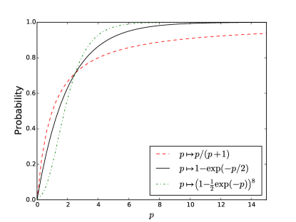
Figure 2: Examples of different success probability functions

2.2 System Dynamics and Costs

The transmitter is modeled as a packet buffer (job queue) with a single transmitter (server). When a packet reaches the head-of-line (HOL) it is assigned a residual deadline $d=D$. The transmitter chooses a power $p$ from a finite set $\mathcal{P}\subseteq\mathbb{R}_{\geq 0}$ and transmits the packet. Assuming the interference state is $i$, with probability $s(p,i)$ the transmission is successful. In this case, the receiver will send an acknowledgment (ACK) to the transmitter over a low rate control channel. The transmission is unsuccessful with probability $1-s(p,i)$. In this case, the receiver sends a negative acknowledgment (NACK), the residual deadline $d$ is decremented by one, and the transmitter reattempts the transmission. This continues until either the packet is successfully transmitted or until the residual deadline reaches zero. When the residual deadline reaches zero, the HOL packet is ejected from the transmitter buffer. The next packet becomes the new HOL packet and is assigned a residual deadline of $D$, as before. Dropping the packet will temporarily degrade the multimedia quality, but prevents jitter and delay. Note that the receiver sends a receiver signal strength indication (RSSI) on the control channel. As a result, we assume that the transmitter knows the current interference state before a transmission power is chosen. This assumption is relaxed in the performance evaluation in Section 5.

As the system evolves, the transmitter incurs the following non-negative costs in each time slot. First, transmitting with power $p\in\mathcal{P}$ costs $\mathcal{C}_{p}(p)$. We assume that $\mathcal{C}_{p}(\cdot)$ is non-decreasing which reflects a natural desire to use less power. Second, the transmitter incurs a backlog cost of $\mathcal{C}_{b}(b)$ when the packet backlog is $b$. We assume that $\mathcal{C}_{b}(\cdot)$ is non-decreasing. This creates what is known in the queueing literature as “backlog pressure” [26]. The backlog pressure reduces the overall latency experienced by the sequence of packets. Finally, when a HOL packet is dropped because the residual deadline reaches zero, the transmitter incurs a constant cost of $\mathcal{C}_{d}$. This cost reflects an aversion to degrading the multimedia stream.

In general, we will use subscripts to indicate time slots. For the packet backlog, assume $b_{0}=B$ and that the backlog at time $t$ is $b_{t}\in\{0,1,2,\ldots,B\}$ for all $t\geq 1$. The residual deadline at time $t$ is $d_{t}\in\{1,2,\ldots,D\}$. The power level at time $t$ (for now chosen according to some arbitrary rule) is $p_{t}\in\mathcal{P}$ and the interference level at time $t$ is $i_{t}$. Let $S_{t}$ be a binary random variable representing the channel so that $\mathbb{P}(S_{t}=0)=1-s(p_{t},i_{t})$ and $\mathbb{P}(S_{t}=1)=s(p_{t},i_{t})$. Using $S_{t}$, we can write the cost in each time slot as follows:

$$g(b_{t},d_{t},i_{t},p_{t})=\mathbb{I}_{\{b_{t}>0\}}\left(\mathcal{C}_{p}(p_{t})+\mathcal{C}_{b}(b_{t})+\mathbb{I}_{\{S_{t}=0\}}\mathbb{I}_{\{d_{t}=1\}}\mathcal{C}_{d}\right)$$ (1)

The dynamics and costs are summarized in Figure 1. Recall that the interference fluctuates independently of all other aspects of the model and therefore $i_{t+1}$ is not influenced by $S_{t}$, $b_{t}$, or $d_{t}$.

	Stage Cost	State Transition
$S_{t}=1$, $b_{t}>0$	$\mathcal{C}_{p}(p_{t})+\mathcal{C}_{b}(b_{t})$	$(b_{t+1},d_{t+1},i_{t+1})=(b_{t}-1,D,i_{t+1})$
$S_{t}=0$, $d_{t}>1,b_{t}>0$	$\mathcal{C}_{p}(p_{t})+\mathcal{C}_{b}(b_{t})$	$(b_{t+1},d_{t+1},i_{t+1})=(b_{t},d_{t}-1,i_{t+1})$
$S_{t}=0$, $d_{t}=1,b_{t}>0,$	$\mathcal{C}_{p}(p_{t})+\mathcal{C}_{b}(b_{t})+\mathcal{C}_{d}$	$(b_{t+1},d_{t+1},i_{t+1})=(b_{t}-1,D,i_{t+1})$
$b_{t}=0$	0	Terminal State

Table 1: A table summarizing the costs and dynamics of the model. $S_{t}$ is a binary variable indicating whether the transmission in time slot $t$ is successful (1 if successful, 0 otherwise). $\mathcal{C}_{p}(\cdot)$ and $\mathcal{C}_{b}(\cdot)$ are non-decreasing costs on the power and backlog respectively. $\mathcal{C}_{d}$ is a constant cost incurred when a deadline is violated. Note that when $b_{t}=0$, the transmission is complete.

There are some modeling aspects that we have chosen to exclude. For example, we have not included a packet arrival process because we are primarily interested in the transmission problem and hence focus on the media packets that are already present at the transmitter. This also reflects the initial motivation of a device transmitting a cached video to another nearby user – the video is already completely stored and there are no arrivals in this case.

Another potential modeling aspect would be non-uniform deadlines. In previous work [20], we allowed for the deadlines to be a function of the backlog so that $D=D(b)$. The following mathematical results still hold, but it is not clear that there is any practical benefit to having backlog adaptive deadlines. For simplicity of exposition, we assume that every packet has the same HOL deadline.

An alternative model could include deadlines for every job rather than just for the HOL packet. Tracking all packet deadlines would cause the state space to explode and the “curse of dimensionality” [27] would yield such a problem numerically intractable. This issue is discussed more in Section 2.4. Furthermore, the HOL deadline allows us to control inter-packet jitter and leads to more regularity in the received packet stream. For applications like multimedia streaming, this will lead to fewer video freezes and a more consistent user experience at the receiver.

We should note that wireless video streaming involves many technical issues such as error correction coding across multiple packets. For example, packet level forward error correction was experimentally investigated by Alay et al. [28]. They designed an application layer mechanism to strategically insert parity packets, thus allowing up to 50% packet loss of video streams over wireless channels with virtually no loss of quality. Hence, we can assume that the receiver can recover the information in the packets that are dropped due to the HOL deadlines. With this experimental work in mind, our model is built to spotlight the theoretical trade-off between transmitter power, packet drop rate (due to missed deadlines), and backlog, which is key in these systems.

2.3 Optimal Control Formulation

Given the Markovian nature of our model, we can now pose the power control problem as a Markov Decision Process (MDP) [27]. At time $t\in\{0,1,2,\ldots\}$, our state is given by $x_{t}=(b_{t},d_{t},i_{t})$. In each time slot, a control policy uses the state to choose a power level for transmission. Mathematically, our set of admissible policies is

$$\Pi=\{\pi:\{1,\ldots,B\}\times\{1,\ldots,D\}\times\{1,\ldots,I\}\rightarrow\mathcal{P}\}.$$ (2)

We want to minimize the total expected cost. Since there is no arrival process, the state $(0,d,i)$ is a terminal state with zero cost for any $(d,i)$. It can take no more than $BD$ time slots to reach the class of terminal states. Therefore, the optimal expected cost-to-go $\mathcal{J}(b,d,i)$ is well-defined:

$$\mathcal{J}(b,d,i)=\min_{\pi\in\Pi}\mathbb{E}\left[\left.\sum_{t=0}^{\infty}g(b_{t},d_{t},i_{t},\pi(b_{t},d_{t},i_{t}))\right|(b_{0},d_{0},i_{0})=(b,d,i)\right]$$ (3)

Note that in (3), the minimization is implicitly subject to the dynamics from Sections 2.1 and 2.2. The dynamics along with the costs give us the following Bellman equation:

$$\begin{split}\mathcal{J}(b,d,i)&=\min_{p\in\mathcal{P}}\Bigg{\{}\mathcal{C}_{b}(b)+\mathcal{C}_{p}(p)\\ &+\sum_{j}P_{ij}\Big{[}s(p,i)\mathcal{J}(b-1,D,j)+(1-s(p,i))(\mathbb{I}_{\{d=1\}}(\mathcal{C}_{d}+\mathcal{J}(b-1,D,j))+\mathbb{I}_{\{d>1\}}\mathcal{J}(b,d-1,j))\Big{]}\Bigg{\}}\end{split}$$ (4)

For each $(b,d,i)$, the minimizer is not necessarily unique so there may be multiple optimal policies. We refer to the optimal policy $\mu$ as the policy defined by the following minimization:

$$\begin{split}\mu(b,d,i)&=\min\operatorname*{argmin}_{p\in\mathcal{P}}\Bigg{\{}\mathcal{C}_{b}(b)+\mathcal{C}_{p}(p)\\ &+\sum_{j}P_{ij}\Big{[}s(p,i)\mathcal{J}(b-1,D,j)+(1-s(p,i))(\mathbb{I}_{\{d=1\}}(\mathcal{C}_{d}+\mathcal{J}(b-1,D,j))+\mathbb{I}_{\{d>1\}}\mathcal{J}(b,d-1,j))\Big{]}\Bigg{\}}\end{split}$$ (5)

The $\operatorname*{argmin}$ operator returns the set of minimizers and $\mu$ is defined by taking the smallest minimizer. Therefore, $\mu$ is the optimal policy which uses the smallest amount of power.

2.4 Practical Drawbacks of Optimal Control

In principle, given the model, we can solve (4) and (5) with standard algorithms like value iteration and policy iteration [27] offline and then store $\mu$ as a look-up table for use online. However, there are some practical limitations to this approach. The algorithmic complexity of computing $\mu$ grows exponentially with the dimension of the state-space so it can become difficult to compute the optimal power control for large numbers of packets and large numbers of interference states. In dynamic programming, this is known as the “curse of dimensionality” [27]. If the system parameters change, (4) and (5) would have to be solved again online, which would not be tractable. In addition, naively storing $\mu$ would require $O(BDI)$ memory which would be prohibitive for large packet buffers.

There are also problems with estimating a model in the first place. Although finite-state Markov interference patterns are a useful model [23], it can be difficult to estimate the transition matrix $P$. First, there is the question of choosing quantization levels. Because of the algorithmic complexity mentioned above, there is a trade-off between model fidelity and ease of computation. In addition, as we increase $I$, the “stochastic complexity” [29] of estimating the model increases. In brief, the number of parameters to be estimated is $O(I^{2})$ and the number of observations needed for reliable estimation grows exponentially with the number of parameters. Finally, note that the finite-state Markov channel is a good stochastic model for interference fluctuating over time, but it does not necessarily capture the notion of fluctuations over space. In particular, interference patterns can be very different in different places which would require estimating new models as mobile users move to new locations.

3 An Illustrative Case

Because of the practical limitations of the general optimal control approach, we instead consider a special case with fixed interference. This corresponds to taking $I=1$. The goal is to mathematically understand the structure of the special case and use this understanding to overcome the aforementioned complexity issues in the general case. We continue to use $\mathcal{J}$ to represent the expected cost-to-go and $\mu$ to represent the optimal policy, but we no longer include the third argument because the interference is constant. We continue to keep interference as the second argument to $s(\cdot,\cdot)$. The new Bellman equation is given below:

$$\begin{split}\mathcal{J}(b,d)=\min_{p\in\mathcal{P}}\Big{\{}&\mathcal{C}_{b}(b)+\mathcal{C}_{p}(p)\\ &+s(p,i)\mathcal{J}(b-1,D)+(1-s(p,i))(\mathbb{I}_{\{d=1\}}(\mathcal{C}_{d}+\mathcal{J}(b-1,D))+\mathbb{I}_{\{d>1\}}\mathcal{J}(b,d-1))\Big{\}}\end{split}$$ (6)

First we numerically explore the optimal power control of this special case. We demonstrate and explain the salient features of the optimal policy. Then we move on to prove theoretical properties of the optimal policy. The theoretical results in this section will be used to design a power control scheme which approximates the optimal control.

3.1 Numerical Results

In this section we fix the following parameters while varying $\mathcal{C}_{d}$: $\mathcal{P}=\{2,4,6\}$, $s(p,i)=1-\exp(-p/2)$, $\mathcal{C}_{b}(b)=b$, $\mathcal{C}_{p}(p)=p$, $B=20$, $D=5$. Varying $\mathcal{C}_{d}$ corresponds to varying the aversion to dropping a packet relative to the other costs. A low value of $\mathcal{C}_{d}$ corresponds to accepting a low quality stream while a high value of $\mathcal{C}_{d}$ corresponds to requiring a high fidelity stream. These parameters do not reflect a particular physical system but are intended to illustrate the features of $\mu$.

In Figure 3, we plot $\mu$ for $\mathcal{C}_{d}\in\{1,10,100\}$. For each $(b,d)\in\{1,2,\ldots,B\}\times\{1,2,\ldots,D\}$, we plot a point indicating $\mu(b,d)\in\mathcal{P}$. We first note that for all values of $\mathcal{C}_{d}$ and each $d$, $b\mapsto\mu(b,d)$ is non-decreasing. This is expected because the backlog pressure incentivizes the transmitter to “try harder” to transmit the packets.

Varying $\mathcal{C}_{d}$ does cause qualitatively different behavior of $d\mapsto\mu(b,d)$. When $\mathcal{C}_{d}=1$, $d\mapsto\mu(b,d)$ is non-decreasing for every $b$. This shows that when the cost of dropping a packet is low, the transmitter will “give up” as the deadline approaches. In contrast, when $\mathcal{C}_{d}=100$, $d\mapsto\mu(b,d)$ is non-increasing for every $b$. In this case, the cost of dropping a packet is high so the transmitter “tries harder” as the deadline approaches. When $\mathcal{C}_{d}=10$, we see that the “give up” and “try harder” behavior depends on the value of $b$. Indeed for $\mathcal{C}_{d}=10$, the policy adopts a “try harder” behavior for low values of $b$ and a “give up” behavior for large values of $b$. In the following section, we analytically determine the relationship between the costs that causes this qualitatively different behavior.

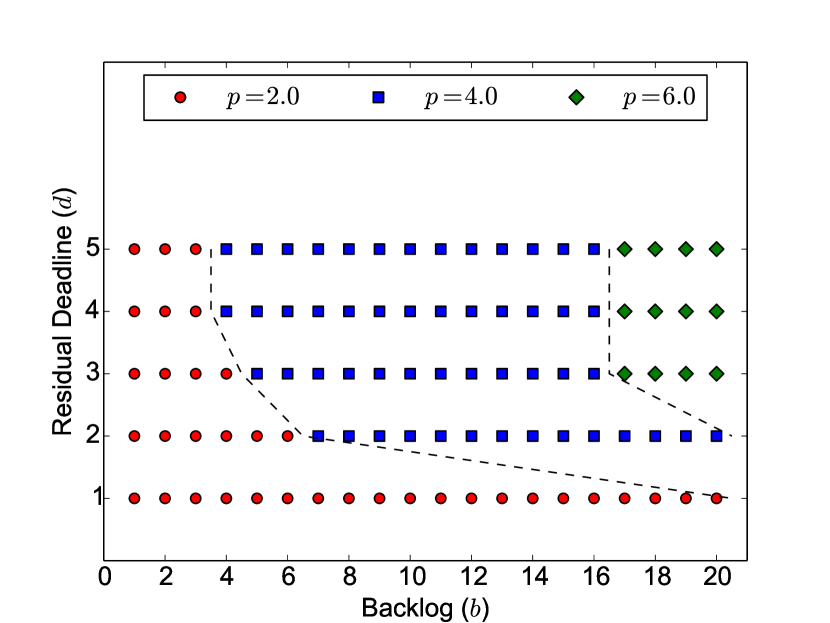
(a) $\mathcal{C}_{d}=1$

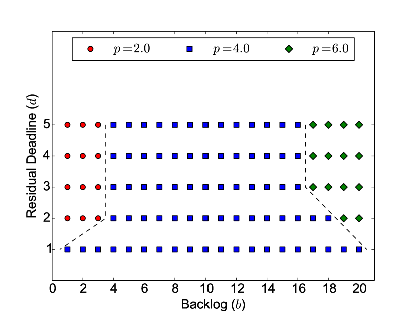
(b) $\mathcal{C}_{d}=10$

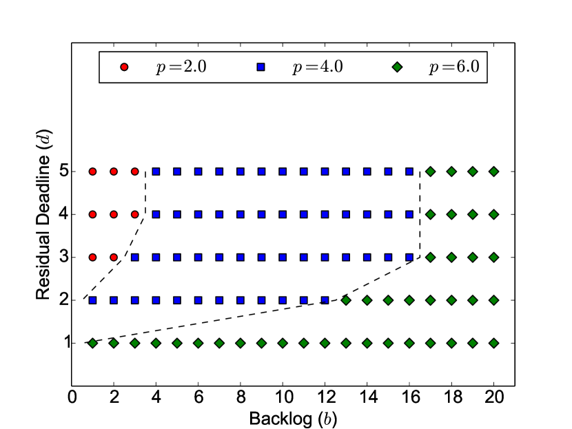
(c) $\mathcal{C}_{d}=100$

Figure 3: Example policies for the illustrative case presented in Section 3. We take $\mathcal{P}=\{2,4,6\}$, $s(p,i)=1-\exp(-p/2)$, $\mathcal{C}_{b}(b)=b$, $\mathcal{C}_{p}(p)=p$, $B=20$, $D=5$ and vary $\mathcal{C}_{d}$. For each $(b,d)\in\{1,2,\ldots,B\}\times\{1,2,\ldots,D\}$, we plot a point indicating $\mu(b,d)\in\mathcal{P}$. The dashed lines indicate partitions in the state space that separate the different power values. For any $\mathcal{C}_{d}$ and any $d$, we see that $b\mapsto\mu(b,d)$ is non-decreasing. However, varying $\mathcal{C}_{d}$ does affect how $\mu(b,d)$ varies with $d$. When $\mathcal{C}_{d}$ is low ($\mathcal{C}_{d}=1$), $d\mapsto\mu(b,d)$ is non-decreasing for every $b$. When $\mathcal{C}_{d}$ is high ($\mathcal{C}_{d}=100$), $d\mapsto\mu(b,d)$ is non-increasing for every $b$. When $\mathcal{C}_{d}$ is moderate ($\mathcal{C}_{d}=10$), $d\mapsto\mu(b,d)$ is non-decreasing for certain values of $b$ and non-increasing for others.

3.2 Theoretical Results

The main results can be summarized informally as follows:

• For any $s(\cdot,\cdot)$, $b\mapsto\mu(b,d)$ is non-decreasing.

• For any $s(\cdot,\cdot)$, if $\mathcal{C}_{b}(b)+\min_{p\in\mathcal{P}}\{\mathcal{C}_{p}(p)-s(p,i)\mathcal{C}_{d}\}\geq 0$ then $d\mapsto\mu(b,d)$ is non-decreasing.

• For any $s(\cdot,\cdot)$, if $\mathcal{C}_{b}(b)+\min_{p\in\mathcal{P}}\{\mathcal{C}_{p}(p)-s(p,i)\mathcal{C}_{d}\}\leq 0$ then $d\mapsto\mu(b,d)$ is non-increasing.

• When $p\mapsto s(p,i)$ is concave or sigmoidal and $\mathcal{C}_{p}(\cdot)$ is linear, $b\mapsto\mu(b,d)$ is well-approximated by a sublinear function of $\mathcal{C}_{b}(b)$. Roughly speaking, the optimal transmitter power grows sublinearly with the backlog cost.

To rigorously prove these theoretical results, we need to apply the following theorem (a version of what is known as Topkis’s Theorem [30]) which is standard in the stochastic dynamic programming literature, e.g. [27].

Theorem 1.

Take some finite $\mathcal{Y}\subseteq\mathbb{R}$. We say $f:\mathbb{R}\times\mathcal{Y}\rightarrow\mathbb{R}$ is submodular if for any $x^{-}\leq x^{+}$ and $y^{-}\leq y^{+}$, the following inequality holds:

$$f(x^{+},y^{+})+f(x^{-},y^{-})\leq f(x^{+},y^{-})+f(x^{-},y^{+})$$ (7)

Let $g(x)=\min\operatorname*{argmin}_{y\in\mathcal{Y}}f(x,y)$. If $f$ is submodular then $g$ is non-decreasing.

Theorem 1 and its generalizations have been used to prove monotonicity properties of MDPs in the queueing and control literature (e.g. [31], [32], and [33]). However, the HOL deadlines in our model prevent us from directly applying these previous results. As seen in Section 3.1, the monotonicity of the optimal control policy varies with the backlog. As a result, we need to approach this problem from first principles. We begin with some definitions and notation which will allow us to reformulate the Bellman equation in (6).

Definition 1.

We define the following auxiliary quantities. For each $b\geq 1$,

$$\delta(b,1)=\mathcal{C}_{b}(b)+\min_{p\in\mathcal{P}}\left\{\mathcal{C}_{p}(p)-s(p,i)\mathcal{C}_{d}\right\}.$$

For $d>1$, $\delta(b,d)$ is inductively defined as follows:

$$\delta(b,d) =\mathcal{C}_{b}(b)+\min_{p\in\mathcal{P}}\left\{\mathcal{C}_{p}(p)-s(p,i)\left(\mathcal{C}_{d}+\sum_{k=1}^{d-1}\delta(b,k)\right)\right\}$$ (8)

In addition, we define $\sigma(b,d)=\sum_{k=1}^{d}\delta(b,k)$. For each of these definitions, whenever the upper limit on a sum is less than the lower limit, the sum is equal to zero.

For $b\geq 1$ we define the operator $T_{b}:\mathbb{R}\rightarrow\mathbb{R}$ as follows:

$$T_{b}(x)=x+\mathcal{C}_{b}(b)+\min_{p\in\mathcal{P}}\left\{\mathcal{C}_{p}(p)-s(p,i)(\mathcal{C}_{d}+x)\right\}$$

Note that $T_{b}(0)=\mathcal{C}_{b}(b)+\min_{p\in\mathcal{P}}\left\{\mathcal{C}_{p}(p)-s(p,i)\mathcal{C}_{d}\right\}$. Therefore, we will be using the sign of $T_{b}(0)$ to tell us whether $\mu(b,\cdot)$ is increasing or decreasing. This idea is further elucidated in the following propositions.

Proposition 1.

For $b\geq 1$, the Bellman equation in (6) can be reformulated as follows:

$$\begin{split}\mathcal{J}(b,d)&=\left\{\begin{array}[]{ll}\mathcal{C}_{d}+\mathcal{J}(b-1,D)+\delta(b,1)&,d=1\\ \mathcal{J}(b,d-1)+\delta(b,d)&,d>1\end{array}\right.\end{split}$$ (9)

Consequently, the optimal policy can we written as

$$\mu(b,d) =\min\operatorname*{argmin}_{p\in\mathcal{P}}\left\{\mathcal{C}_{p}(p)-s(p,i)(\mathcal{C}_{d}+\sigma(b,d-1))\right\}.$$ (10)

Also note that since every cost is non-negative, $\mathcal{J}(b,d)\geq 0$ for every $(b,d)$.

Proof.

We apply the principle of strong mathematical induction. For $d=1$, this is just a reordering of the terms in the Bellman equation. For $d=2$, we have the following:

$$\mathcal{J}(b,2) =\min_{p\in\mathcal{P}}\{\mathcal{C}_{p}(p)+\mathcal{C}_{b}(b)+s(p,i)\mathcal{J}(b-1,D)+(1-s(p,i))\mathcal{J}(b,1)\}$$ (11)

$$=\mathcal{J}(b,1)+\mathcal{C}_{b}(b)+\min_{p\in\mathcal{P}}\{\mathcal{C}_{p}(p)-s(p,i)(\mathcal{J}(b,1)-\mathcal{J}(b-1,D))\}$$ (12)

$$=\mathcal{J}(b,1)+\mathcal{C}_{b}(b)+\min_{p\in\mathcal{P}}\{\mathcal{C}_{p}(p)-s(p,i)(\mathcal{C}_{d}+\delta(b,1))\}$$ (13)

$$=\mathcal{J}(b,1)+\delta(b,2)$$ (14)

Now assume the proposition is true for all $d-1,d-2,d-3,\ldots,2,1$.

$$\mathcal{J}(b,d)$$

$$=\min_{p\in\mathcal{P}}\{\mathcal{C}_{p}(p)+\mathcal{C}_{b}(b)+s(p,i)\mathcal{J}(b-1,D)+(1-s(p,i))\mathcal{J}(b,d-1)\}$$ (15)

$$=\mathcal{J}(b,d-1)+\mathcal{C}_{b}(b)+\min_{p\in\mathcal{P}}\{\mathcal{C}_{p}(p)-s(p,i)(\mathcal{J}(b,d-1)-\mathcal{J}(b-1,D))\}$$ (16)

$$=\mathcal{J}(b,d-1)+\mathcal{C}_{b}(b)+\min_{p\in\mathcal{P}}\left\{\mathcal{C}_{p}(p)-s(p,i)\left(\sum_{k=2}^{d-1}(\mathcal{J}(b,k)-\mathcal{J}(b,k-1))+\mathcal{J}(b,1)-\mathcal{J}(b-1,D)\right)\right\}$$ (17)

$$=\mathcal{J}(b,d-1)+\mathcal{C}_{b}(b)+\min_{p\in\mathcal{P}}\left\{\mathcal{C}_{p}(p)-s(p,i)\left(\sum_{k=2}^{d-1}\delta(b,k)+\mathcal{J}(b,1)-\mathcal{J}(b-1,D)\right)\right\}$$ (18)

$$=\mathcal{J}(b,d-1)+\mathcal{C}_{b}(b)+\min_{p\in\mathcal{P}}\left\{\mathcal{C}_{p}(p)-s(p,i)\left(\mathcal{C}_{d}+\sum_{k=1}^{d-1}\delta(b,k)\right)\right\}$$ (19)

$$=\mathcal{J}(b,d-1)+\delta(b,d)$$ (20)

In (17), we replace $\mathcal{J}(b,d-1)$ with an equivalent telescoping sum. This allows us to apply the induction hypothesis in (18) and (19).

This reformulation of the Bellman equation allows us to just ignore the terms that don’t involve $p$ to see that

$$\mu(b,d)=\min\operatorname*{argmin}_{p\in\mathcal{P}}\left\{\mathcal{C}_{p}(p)-s(p,i)\left(\mathcal{C}_{d}+\sum_{k=1}^{d-1}\delta(b,k)\right)\right\}.$$

Replacing the sum with $\sigma(b,d-1)$ completes the proof. ∎

This gives us a semi-analytic expression for $\mu$. In other words, we now have an expression for $\mu$ which depends on $\sigma$ rather than on $\mathcal{J}$. We will use the $\delta$ terms to determine whether $\sigma(b,d)$ is increasing or decreasing in $b$ and/or $d$.

Proposition 2.

For each $b$, $T_{b}(\cdot)$ is non-decreasing. We can write $\sigma(b,d)=T_{b}(\sigma(b,d-1))$ where $\sigma(b,0)=0$. For $d\geq 1$ and $b\geq 1$ we have the following conditions:

• For each $d$, $\sigma(\cdot,d)$ is non-decreasing.

• If $T_{b}(0)\geq 0$ then $\sigma(b,\cdot)$ is non-negative and non-decreasing.

• If $T_{b}(0)\leq 0$ then $\sigma(b,\cdot)$ is non-positive and non-increasing.

Proof.

Take $x\geq y$. For any $p$, $(1-s(p,i))\geq 0$ so $(1-s(p,i))x\geq(1-s(p,i))y$. Adding terms to both sides preserves the inequality so

$$\mathcal{C}_{b}(b)+(1-s(p,i))x+\mathcal{C}_{p}(p)-s(p,i)\mathcal{C}_{d}\geq\mathcal{C}_{b}(b)+(1-s(p,i))y+\mathcal{C}_{p}(p)-s(p,i)\mathcal{C}_{d}.$$ (21)

Taking the minimum over $p\in\mathcal{P}$ and using the monotonicity of minimization gives us that $T_{b}(x)\geq T_{b}(y)$.

We originally defined $\sigma(b,d)=\sum_{k=1}^{d}\delta(b,k)$. If $d=0$ then the sum is vacuous so $\sigma(b,0)=0$. For $d\geq 1$,

$$\sigma(b,d) =\sum_{k=1}^{d}\delta(b,k)=\sum_{k=1}^{d-1}\delta(b,k)+\delta(b,d)=\sigma(b,d-1)+\delta(b,d)$$ (22)

$$=\sigma(b,d-1)+\mathcal{C}_{b}(b)+\min_{p\in\mathcal{P}}\left\{\mathcal{C}_{p}(p)-s(p,i)\left(\mathcal{C}_{d}+\sum_{k=1}^{d-1}\delta(b,k)\right)\right\}$$ (23)

$$=\sigma(b,d-1)+\mathcal{C}_{b}(b)+\min_{p\in\mathcal{P}}\left\{\mathcal{C}_{p}(p)-s(p,i)\left(\mathcal{C}_{d}+\sigma(b,d-1)\right)\right\}$$ (24)

$$=T_{b}(\sigma(b,d-1))$$ (25)

Since $\mathcal{C}_{b}(\cdot)$ is non-decreasing, $T_{b^{\prime}}(x)\geq T_{b}(x)$ for any $b^{\prime}\geq b$. Since $\sigma(b,d)$ can be found by iteratively applying $T_{b}(\cdot)$ to $0$, we have that $\sigma(b^{\prime},d)\geq\sigma(b,d)$ for any $b^{\prime}\geq b$. Therefore, $\sigma(\cdot,d)$ is non-decreasing for all $d$.

Now we show how $\sigma(b,d)$ varies with $d$. Assume that $T_{b}(0)\geq 0$ and proceed by induction. $\sigma(b,0)=0$ so we have that $\sigma(b,1)=T_{b}(\sigma(b,0))\geq\sigma(b,0)$. If $\sigma(b,d)\geq\sigma(b,d-1)$ then applying $T_{b}$ and using the fact that $T_{b}$ is non-decreasing gives us that

$$\sigma(b,d+1)=T_{b}(\sigma(b,d)) \geq T_{b}(\sigma(b,d-1))=\sigma(b,d)$$ (26)

Therefore, $\sigma(b,\cdot)$ is non-decreasing for all $d$. $\sigma(b,0)=0$ so $\sigma(b,d)$ is non-negative. The case of $T_{b}(0)\leq 0$ is analogous. ∎

Now that we understand the monotonicity properties of $\sigma(b,d)$, we can leverage these to understand the monotonicity properties of $\mu(b,d)$.

Proposition 3.

The optimal policy $\mu(b,d)$ is always non-decreasing in $b$. If $T_{b}(0)\geq 0$ then $\mu(b,d)$ is non-decreasing in $d$. If $T_{b}(0)\leq 0$ then $\mu(b,d)$ is non-increasing in $d$.

Proof.

We can now leverage Theorem 1 for our specific problem. From Proposition 1,

$$\mu(b,d)=\min\operatorname*{argmin}_{p\in\mathcal{P}}\left\{\mathcal{C}_{p}(p)-s(p,i)(\mathcal{C}_{d}+\sigma(b,d-1))\right\}.$$

Let $f(x,p)=\mathcal{C}_{p}(p)-s(p,i)x$ and define $g(x)$ as in Theorem 1 with $\mathcal{Y}=\mathcal{P}$. Then $\mu(b,d)=g(\mathcal{C}_{d}+\sigma(b,d-1))$. Let LHS and RHS be the left-hand side and right-hand side of (7).

$$LHS -RHS$$

$$=\left(\mathcal{C}_{p}(p^{+})-s(p^{+},i)x^{+}+\mathcal{C}_{p}(p^{-})-s(p^{-},i)x^{-}\right)-\left(\mathcal{C}_{p}(p^{+})-s(p^{+},i)x^{-}+\mathcal{C}_{p}(p^{-})-s(p^{-},i)x^{+}\right)$$ (27)

$$=(s(p^{+},i)-s(p^{-},i))(x^{-}-x^{+})$$ (28)

By assumption, $(s(p^{+},i)-s(p^{-},i))\geq 0$ while $(x^{-}-x^{+})\leq 0$ so $LHS\leq RHS$. Therefore, $f$ is submodular, $g$ is non-decreasing, and $\mu(b,d)$ is a non-decreasing function of $\sigma(b,d-1)$.

$\sigma(b,d)$ is non-decreasing in $b$ so $\mu(b,d)$ is non-decreasing in $b$. If $T_{b}(0)\geq 0$ then $\sigma(b,d)$ is non-decreasing in $d$ so $\mu(b,d)$ is non-decreasing in $d$. If $T_{b}(0)\leq 0$ then $\sigma(b,d)$ is non-increasing in $d$ so $\mu(b,d)$ is non-increasing in $d$. ∎

In order to understand more precisely how $\mu(b,d)$ increases with $b$, we need to understand more precisely how $\sigma(b,d)$ increases with $b$. The following result gives us that understanding.

Proposition 4.

Let $m=\min_{p\in\mathcal{P}}\{\mathcal{C}_{p}(p)-s(p,i)\mathcal{C}_{d}\}$ and $M=\max_{p\in\mathcal{P}}\{\mathcal{C}_{p}(p)-s(p,i)\mathcal{C}_{d}\}$. Let $s_{min}=s(\min\mathcal{P},i)$ and $s_{max}=s(\max\mathcal{P},i)$. For any fixed $b$ and $d$, we have the following cases:

• $T_{b}(0)>0$:

  $$\left(\mathcal{C}_{b}(b)+m\right)\sum_{k=0}^{d-1}(1-s_{max})^{k}\leq\sigma(b,d)\leq\left(\mathcal{C}_{b}(b)+M\right)\sum_{k=0}^{d-1}(1-s_{min})^{k}$$ (29)

• $T_{b}(0)<0$:

  $$\left(\mathcal{C}_{b}(b)+m\right)\sum_{k=0}^{d-1}(1-s_{min})^{k}\leq\sigma(b,d)\leq\left(\mathcal{C}_{b}(b)+M\right)\sum_{k=0}^{d-1}(1-s_{max})^{k}$$ (30)

• $T_{b}(0)=0$:

  $$\sigma(b,d)=0$$ (31)

Proof.

By substituting the optimal policy into the minimization in $T_{b}$ we have

$$\sigma(b,d+1) =T_{b}(\sigma(b,d))=\sigma(b,d)+\mathcal{C}_{b}(b)+\min_{p\in\mathcal{P}}\left\{\mathcal{C}_{p}(p)-s(p,i)(\mathcal{C}_{d}+\sigma(b,d))\right\}$$ (32)

$$=\sigma(b,d)+\mathcal{C}_{b}(b)+\mathcal{C}_{p}(\mu(b,d))-s(\mu(b,d),i)(\mathcal{C}_{d}+\sigma(b,d))$$ (33)

$$=(1-s(\mu(b,d),i))\sigma(b,d)+\mathcal{C}_{b}(b)+\mathcal{C}_{p}(\mu(b,d))-s(\mu(b,d),i)\mathcal{C}_{d}$$ (34)

Consider the case when $T_{b}(0)>0$ so that $\sigma(b,d)>0$. By first optimizing $\mathcal{C}_{p}(p)-s(p,i)\mathcal{C}_{d}$ over $p\in\mathcal{P}$ and then optimizing $(1-s(p,i))$ over $p\in\mathcal{P}$, we have the following inequality:

$$(1-s_{max})\sigma(b,d)+\mathcal{C}_{b}(b)+m\leq\sigma(b,d+1)\leq(1-s_{min})\sigma(b,d)+\mathcal{C}_{b}(b)+M$$ (35)

For $d=1$, the condition holds because $\mathcal{C}_{b}(b)+m=\sigma(b,1)\leq\mathcal{C}_{b}(b)+M$. If the condition holds for $\sigma(b,d)$ then we have that

$$\sigma(b,d+1) \leq(1-s_{min})\sigma(b,d)+\mathcal{C}_{b}(b)+M\leq(1-s_{min})\left((\mathcal{C}_{b}(b)+M)\sum_{k=0}^{d-1}(1-s_{min})^{k}\right)+\mathcal{C}_{b}(b)+M$$ (36)

$$=(\mathcal{C}_{b}(b)+M)\sum_{k=0}^{d}(1-s_{min})^{k}.$$ (37)

We can apply similar reasoning for the lower bound. By induction, the condition holds for all $d$.

The case when $T_{b}(0)<0$ and $\sigma(b,d)<0$ is analogous.

Recall that $\sigma(b,d)$ can be computed by iteratively applying $T_{b}(\cdot)$ to 0. When $T_{b}(0)=0$, we have that $\sigma(b,d)=0$ for all $d$. ∎

Proposition 4 tells us that $b\mapsto\sigma(b,d)$ is bounded above and below by affine functions of $\mathcal{C}_{b}(b)$. Intuitively, the important thing to note is that for any fixed $d$, $\sigma(b,d)$ is roughly proportional to $\mathcal{C}_{b}(b)$. For example, in the degenerate case when $\mathcal{P}$ is a singleton, the upper and lower bounds are equal and $\sigma(b,d)$ is an affine function of $\mathcal{C}_{b}(b)$. Furthermore, the inequalities hold for any $b$ no matter how large $B$ is.

In the previous propositions, we only assumed that $\mathcal{C}_{p}(\cdot)$ and $s(\cdot,i)$ were non-decreasing. Now we consider when $\mathcal{C}_{p}(\cdot)$ is linear and $s(\cdot,i)$ is concave. Assuming $\mathcal{C}_{p}(\cdot)$ is linear is somewhat limiting, but linear power costs form an important class that has been considered in the communications engineering literature (e.g. [34, 35]) as well as in the information theory literature (e.g. [36]). In addition, although assuming $s(\cdot,i)$ is concave may seem limiting, we will use this as a step towards considering a much broader class of success probability functions. We also introduce the following definition which allows us to precisely state the necessary result.

Definition 2.

We say a non-negative real-valued function $f$ is sublinear if

1. there exists $K_{1},K_{2}\in(0,\infty)$ such that $K_{1}x+K_{2}\geq f(x)$ for all $x\geq 0$, and

2. the asymptotic behavior of $f$ is such that

   $$\lim_{x\rightarrow\infty}\frac{f(x)}{x}=0.$$

This definition differs slightly from the standard computer science definition of sublinearity [37] which would only require the second condition. The second condition only considers the asymptotic behavior of the function while the first condition also captures the behavior over finite subsets of the domain. This is important in our application because we are minimizing over a finite set of power values $\mathcal{P}$.

Proposition 5.

Consider the following function:

$$\gamma(b,d)=\operatorname*{argmin}_{p\geq 0}\{\mathcal{C}_{p}(p)-s(p,i)(\mathcal{C}_{d}+\sigma(b,d-1))\}$$

Assume $\mathcal{C}_{p}(p)=Kp$ for some $K>0$ and that for some function $\phi:[0,\infty)\rightarrow[0,\infty)$ that is differentiable, strictly increasing, and convex function, that $\frac{\partial}{\partial p}s(p,i)=\frac{1}{\phi(p,i)}$. Then, $\gamma(b,d)$ is a sublinear function of $\sigma(b,d-1)$.

Proof.

First assume that $\mathcal{C}_{d}+\sigma(b,d-1)\geq 0$. This is always the case when $T_{b}(0)\geq 0$. The function being minimized is convex so the first-order optimality condition is both necessary and sufficient.

$$\frac{\partial}{\partial p}\{\mathcal{C}_{p}(p)-s(p,i)(\mathcal{C}_{d}+\sigma(b,d-1))\}=K-s^{\prime}(p,i)(\mathcal{C}_{d}+\sigma(b,d-1))=0\iff s^{\prime}(p,i)=\frac{K}{\mathcal{C}_{d}+\sigma(b,d-1)}$$

$\phi(\cdot,i)$ is strictly increasing so it is invertible. Therefore,

$$\gamma(b,d)=\phi^{-1}\left(\frac{\mathcal{C}_{d}+\sigma(b,d-1)}{K},i\right)$$

where we take the inverse with respect to the first argument. $\phi(\cdot,i)$ is strictly increasing and convex so $\phi^{-1}(\cdot,i)$ is strictly increasing and concave. Therefore, $\phi^{-1}(\cdot,i)$ is sublinear.

When $\mathcal{C}_{d}+\sigma(b,d)<0$, we are minimizing an increasing function so $\gamma(b,d)=0$ which is trivially sublinear. ∎

We now briefly consider how one could adapt Proposition 5 for the case that $s(\cdot,i)$ is sigmoidal. Recall that while concave forms for $s(\cdot,i)$ have been used in the transmitter power control literature (e.g. [24]), sigmoidal forms for $s(\cdot,i)$ have been emperically shown to be more accurate (e.g. [25]). A sigmoidal function of the form $p\mapsto\left(1-\frac{1}{2}\exp\left(-\beta_{0}\frac{p}{i}+\beta_{1}\right)\right)^{\beta_{2}}$ will be strictly convex for smaller values of $p$ and strictly concave for larger values of $p$. As a result, two distinct values of $p$ will satisfy the first-order optimality criterion used in the proof of Proposition 5.

To alleviate this problem, we can adjust the definition of $\gamma(b,d)$. Instead of using

$$\gamma(b,d)=\operatorname*{argmin}_{p\geq 0}\{\mathcal{C}_{p}(p)-s(p,i)(\mathcal{C}_{d}+\sigma(b,d-1))\}$$

we can use

$$\gamma(b,d)=\operatorname*{argmin}_{p\geq 0}\{\mathcal{C}_{p}(p)-s_{ccv}(p,i)(\mathcal{C}_{d}+\sigma(b,d-1))\}$$

where $s_{ccv}(\cdot,i)$ is the concave envelope of $s(\cdot,i)$, i.e.

$$s_{ccv}(\cdot,i)=\inf\{h(\cdot):s(p,i)\leq h(p)\,\forall\,p\geq 0,\,h(\cdot)\hbox{ is concave}\}.$$

The concave envelope of a function is analogous to the convex envelope of a function and such envelopes be used to approximately minimize non-convex (or maximize non-concave) function (see e.g. [38]). However, in this case, using $s_{ccv}(\cdot,i)$ instead of $s(\cdot,i)$ yields an exact result rather than an approximation. Indeed, we are using $s_{ccv}(\cdot,i)$ instead of $s(\cdot,i)$ only in the definition of $\gamma(b,d)$ and not in the definitions of $\delta(b,d)$ or $\sigma(b,d)$. As a result, $s_{ccv}(\cdot,i)$ does not change the minimum but merely makes the first-order optimization condition sufficient for finding this minimum. This is depicted in Figure 4.

Furthermore, for a given sigmoidal function $s(\cdot,i)$, it is easy to compute $s_{ccv}(\cdot,i)$. By definition, $s_{ccv}(\cdot,i)$ is the smallest concave function that majorizes $s(\cdot,i)$. Since $s(\cdot,i)$ is concave for sufficiently large values, there is some $p^{*}$ such that $s_{ccv}(p,i)=s(p,i)$ for all $p\geq p^{*}$. In addition, because $s(\cdot,i)$ is convex for $p\in[0,p^{*}]$, the concave envelope will be linear on $[0,p^{*}]$. Hence,

$$s_{ccv}(p,i)=\left\{\begin{array}[]{cl}K_{ccv}p+s(0,i)&,p\in[0,p^{*})\\ s(p,i)&,p\geq p^{*}\end{array}\right.$$

where $p^{*}\in(0,\infty)$ satisfies

$$s^{\prime}(p^{*},i)=\frac{s(p^{*},i)-s(0,i)}{p^{*}}$$

and $K_{ccv}=s^{\prime}(p^{*},i)$. Figure 4 shows this graphically.

This demonstrates that (with a slight modification) Proposition 5 applies to both concave as well as sigmoidal success probability functions. Proposition 4 tells us that $\sigma(b,d)$ is roughly proportional to $\mathcal{C}_{b}(b)$ so Proposition 5 indicates that $\gamma$ is well-approximated by a sublinear function of $\mathcal{C}_{b}(b)$. Introducing $\phi$ and $\gamma$ allows us to to make use of continuous optimization theory which leads to closed-form results that wouldn’t arise when optimizing over the finite set $\mathcal{P}$. We will see below that $\gamma$ is useful for designing power control schemes.

(a)

(b)

Figure 4: A depiction of how the concave envelope of a sigmoidal success probability function can be used to simplify $\gamma(b,d)$. Figure 4(a) demonstrates how $s_{ccv}(\cdot,i)$ compares to $s(\cdot,i)$. Figure 4(b) shows how using $s_{ccv}(\cdot,i)$ makes the first-order optimality condition sufficient for minimization.

4 Sublinear-Backlog Power Control Algorithm

Now we would like to to leverage the theoretical results above in order to build a low-complexity power control scheme which approximates the original optimal control scheme. Intuitively, these low-complexity power controls are schemes which aim to mimic the behavior of $\mu(b,d,i)$. In Section 2.3, we defined $\Pi$ as the set of deterministic policies but we will see that it can be useful to use a stochastic scheme to capture the prominent structural features proven above. To demonstrate our methodology, we focus on a particular functional form of $s(p,i)$. We consider a linear power cost and present two schemes. The first makes use of the fact that $\mu(b,d)$ grows sublinearly with $\mathcal{C}_{b}(b)$ for any fixed $d$. The second introduces a further refinement which incorporates how $\mu(b,d)$ varies with $d$ and $i$.

4.1 A Particular Success Probability Function

The function $s(\cdot,\cdot)$ characterizes the wireless channel. In Section 2.1, we gave some natural conditions that $s(\cdot,\cdot)$ must satisfy but there is still considerable flexibility available for modeling different types of channels. As discussed above with regard to Propsition 5, our results apply to concave functions like $s(p,i)=p/(p+i)$ and $s(p,i)=1-\exp(p/i)$ and also sigmoidal functions of the form $s(p,i)=\left(1-\frac{1}{2}\exp\left(-\beta_{0}\frac{p}{i}+\beta_{1}\right)\right)^{\beta_{2}}$. To demonstrate the applicability of our results, we choose to focus on a simple form. The same approach can be applied with more complicated functions, but the closed forms involved will be more cumbersome.

With this in mind, consider $s(p,i)=1-\exp(-p/i)$. Using the notation from Proposition 5 gives us that $\phi(p,i)=i\exp(p/i)$. When $T_{b}(0)\geq 0$ and $i=1$,

$$\gamma(b,d) =\ln\left(\frac{\mathcal{C}_{d}+\sigma(b,d-1)}{K}\right),$$ (38)

$$\gamma(b,2) =\ln\left(\frac{\mathcal{C}_{d}+\sigma(b,1)}{K}\right)=\ln\left(\frac{\mathcal{C}_{d}+\mathcal{C}_{b}(b)+\min_{p\in\mathcal{P}}\{\mathcal{C}_{p}(p)-s(p,1)\mathcal{C}_{d}\}}{K}\right).$$ (39)

This demonstrates that the power (roughly) grows logarithmically with the backlog cost and thus justifies the “sublinear-backlog” heuristic that will be utilized in the following schemes.

4.2 Sublinear-Backlog Power Control 1 (SLBPC1)

We first create a power control scheme adapts to the packet backlog, but does not react to approaching deadlines or to fluctuating interference. This gives us a simple policy which is a function of only $b$. The previous calculation suggests that using $\gamma(b,2)$ would be a reasonable approximate policy that meets this requirement. Since $\gamma(b,2)$ takes values in $\mathbb{R}_{\geq 0}$ rather than $\mathcal{P}$, we define $\hat{\gamma}$ as follows:

$$\hat{\gamma}(b)=\min\operatorname*{argmin}_{p\in\mathcal{P}}\left|p-\gamma(b,2)\right|$$ (40)

So SLBPC1 is a deterministic policy defined by $\hat{\gamma}(b)$. This type of sub-optimal policy is useful because it does not require the transmitter to know anything about the current interference. Furthermore, $\hat{\gamma}$ has a simple form which can be easily implemented. On the other hand, SLBPC1 does not adapt to approaching deadlines or to fluctuating interference so it will not behave entirely like the optimal control.

4.3 Sublinear-Backlog Power Control 2 (SLBPC2)

Our second power control scheme builds on SLBPC1 by incorporating our understanding of how to react to interference and approaching deadlines. Recall that for fixed interference, the sign of $T_{b}(0)$ determines whether the optimal policy will increase or decrease power as the deadline approaches. We will now apply this idea to the case of fluctuating interference. Let $f_{b}(i)$ as follows:

$$f_{b}(i)=T_{b}(0)=\mathcal{C}_{b}(b)+\min_{p\in\mathcal{P}}\left\{\mathcal{C}_{p}(p)-s(p,i)\mathcal{C}_{d}\right\}$$ (41)

Define the “signum” function as $\text{sgn}(x)=2\mathbb{I}_{\{x\geq 0\}}-1$. We will use $\text{sgn}(f_{b}(i))$ to stochastically drift the power value up or down as the interference and backlog change. More concretely, LBCP2 is described as follows:

1. When there are $b$ packets in the buffer, the initial power level for a new HOL packet is $\hat{\gamma}(b)$.

2. If the previous transmission attempt is not successful, the transmitter computes $\text{sgn}(f_{b}(i))$. If $\text{sgn}(f_{b}(i))$ is positive, the power is increased to the next highest level with probability $p_{change}$. If $\text{sgn}(f_{b}(i))$ is negative, the power is decreased to the next lowest level with probability $p_{change}$. If a higher/lower power level does not exist and the power needs to be increased/decreased, the power level remains the same.

3. This process is followed until the packet is successfully transmitted or until the deadline is exceeded. The process is then continued with a backlog of $b-1$.

We still need to choose a value for $p_{change}$. The packet will be at the HOL for a number of time slots in $\{1,2,\ldots,D\}$. As a result, $p_{change}$ should be inversely proportional to $D$ so that when $D$ becomes large $p_{change}$ becomes small. This corresponds to the case of not having deadlines and the power control being constant for the packet. In practice, a precise value can be chosen experimentally but we take $p_{change}=1/(2D)$.

SLBPC2 adapts to interference, deadlines, and backlog while SLBPC1 only adapts to backlog. However, this requires an increase in complexity. SLBPC2 needs to store the previous transmission power. SLBPC2 requires a reliable RSSI and also needs to compute $\text{sgn}(f_{b}(i))$. Finally, note that SLBPC2 requires a psuedo-random number generator (PRNG). On the other hand, SLBPC2 is still low complexity when compared to the optimal control. SLBPC2 does not require solving dynamic programming equations and does not require knowledge of the interference transition matrix $P$.

5 Performance Evaluation

We take a two-pronged approach to the performance evaluation. In the first approach, we verify that the SLBPC algorithms perform similarly to the optimal control policy in some simple cases where the optimal control can easily be computed. We then consider a more detailed simulation in which power control is not on the same time scale as the interference dynamics and there are also packet arrivals. In this more detailed setting computing the optimal control is not tractable so we compare SLBPC2 to some benchmark algorithms and show a statistically significant increase in performance.

5.1 Verification

In this performance evaluation, we will compare the following power control schemes:

• DP, the optimal control policy defined by $\mu(b,d,i)$.

• MIN, a benchmark power control scheme which always transmits at the minimum power.

• MAX, a benchmark power control scheme which always transmits at the maximum power.

• SLBPC1, the scheme defined above which does not adapt to deadlines or interference.

• SLBPC2, the scheme defined above which does adapt to approaching deadlines and fluctuating interference.

We will take $B=20$, $D=5$, $\mathcal{C}_{b}(b)=b$, $s(p,i)=1-\exp(p/(2i))$, $\mathcal{P}=\{0.1,0.2,0.4,0.8\}$, and $\mathcal{C}_{d}=1$. We will take $\mathcal{C}_{p}(p)=Kp$ where $K>0$ will be varied to show how the power control schemes are affected by different power sensitivities. Note that these parameters are not meant to describe a specific system. This performance evaluation is meant to illustrate the various trade-offs between the different power control schemes.

We assume the interference takes two possible values $i_{t}\in\{1,2\}$. Let $p_{u}$ be the probability that the interference moves from low to high (i.e. up) and let $p_{d}$ is the probability of the interference moving from high to low (i.e. down). The transition matrix is therefore given by

$$P=\left[\begin{array}[]{cc}1-p_{u}&p_{u}\\ p_{d}&1-p_{d}\end{array}\right].$$ (42)

By varying $p_{u}$ and $p_{d}$, we can simulate slow fading and fast fading channels. In particular, when $p_{u}$ and $p_{d}$ are small, we have a slow fading channel and when $p_{u}$ and $p_{d}$ are large, we have a fast fading channel. It is important to investigate these different cases because SLBPC1 and SLBPC2 were designed with properties from the fixed interference case. Fixed interference can be a good approximation of a slow fading channel but typically not of a fast fading channel.

For each scheme we vary $K$, $p_{u}$, and $p_{d}$ and compute different performance metrics via Monte Carlo simulation with 2000 particles. Because of how we formulated the optimal control problem, the obvious metric is the total cost. In addition, we compute the average fraction of dropped packets and the average power per packet.

5.1.1 Slow Fading

We begin by simulating a slow fading channel in which $p_{u}=p_{d}=0.1$. Because $1/p_{u}=1/p_{d}=10$ and $D=5$, we expect that each packet will only experience a fixed level of interference. We first vary $K$ and plot the estimated total cost incurred by each of the power control schemes. The results are shown in Figure 5(a). When the power sensitivity is low (i.e. small values of $K$), the DP and SLBPC schemes perform like the MAX scheme and when the power sensitivity is high (i.e. large values of $K$), the DP and SLBPC schemes perform like the MIN scheme. For moderate power sensitivities, the DP outperforms both SLBPC schemes but the SLBPC cost curves are qualitatively similar to the DP cost curve. We also see that when it comes to total cost, the SLBPC schemes are almost indistinguishable.

(a) Total Cost vs. Power Sensitivity, Slow Fading

(b) Total Cost vs. Power Sensitivity, Fast Fading

Figure 5: Estimated total cost as a function of power sensitivity. The power cost is $\mathcal{C}_{p}(p)=Kp$ so a lower value of $K$ indicates less sensitivity of power while a higher value of $K$ indicates a greater sensitivity. In the slow fading case, $p_{u}=p_{d}=0.1$. In the fast fading case, $p_{u}=p_{d}=0.9$. For low values of $K$, the DP and SLBPC schemes are just like the MAX scheme. For high values of $K$, the DP and SLBPC schemes are just like the MIN scheme. For moderate values of $K$, both SLBPC schemes qualitatively match the DP scheme. These observations hold for both the slow fading and fast fading cases.

The SLBPC schemes achieve a very similar total cost, but we know that they do not achieve this total cost in the same way. Because the SLBPC2 scheme adapts to interference and deadlines, SLBPC2 behaves more similarly to the DP scheme than SLBPC1 does. To demonstrate this, we choose a few values for $K$ and compute the average power per packet and the average fraction of dropped packets. The results are shown in Figure 6(a). In each case, SLBPC2 is more similar to the DP scheme than SLBPC1 is. SLBPC1 and SLBPC2 may achieve similar total costs, but SLBPC2 is more similar in behavior to the DP scheme.

(a) Performance Metrics for Various $K$, Slow Fading

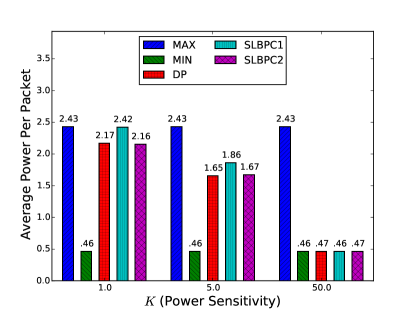
(b) Performance Metrics for Various $K$, Fast Fading

Figure 6: For a few different values of $K$, the schemes are compared on the average fraction of dropped packets and the average power expended per packet. In the slow fading case, $p_{u}=p_{d}=0.1$. In the fast fading case, $p_{u}=p_{d}=0.9$. We see that SLBPC2 behaves more similarly to the DP scheme than SLBPC1 even though the SLBPC schemes have similar total costs. This demonstrates that reacting to deadlines and adapting to fluctuating interference is important when approximating the optimal control.

5.1.2 Fast Fading

Now we consider a fast fading channel for which $p_{u}=p_{d}=0.9$. Because $1/p_{u}=1/p_{d}=1.\overline{11}$ while $D=5$, we expect the interference to change multiple times during the transmission of a single packet. As a result, having knowledge of the interference transition matrix $P$ could give the DP power control scheme a significant advantage over the SLBPC schemes.

However, our simulations show that the SLBPC schemes do not degrade in performance due to a fast fading channel. In Figure 5(b), we plot the total cost as a function of the power sensitivity $K$. As with the slow fading channel, we see that the DP scheme acts like the MAX scheme for low $K$, like the MIN scheme for high $K$, and is better than all schemes for moderate $K$. We also see that the cost curves for the SLBPC schemes are qualitatively similar to the cost curve for the DP scheme. In addition, the optimality gap is not significantly greater than it was in the case of a slow fading channel. Furthermore, when considering the average fraction of dropped packets and the average power per packet in Figure 6(b), we see the same trends as before. Both SLBPC schemes are similar to the DP scheme in terms of total cost, but SLBPC2 is more similar to the DP scheme in terms of behavior.

5.2 Detailed Simulation

In this section we consider a more realistic simulation in which our assumptions do not always hold. We fix $\mathcal{C}_{d}=1$, $\mathcal{C}_{b}(b)=b$, $D=3$, and $\mathcal{P}=\{0.5,1.0,2.0,4.0,8.0\}$. The transmitter starts with $B=100$ packets and in each time slot a new packet arrives with probability $0.1$. We consider a two-state channel where the low interference level is 8.0 and the high interference level is 16.0. The transition matrix for the channel is given by

$$P=\left[\begin{array}[]{cc}0.1&0.9\\ 0.9&0.1\end{array}\right]$$ (43)

so that we have a fast fading channel. In addition, we assume that the channel dynamics are at a time scale that is twice as fast as the transmission dynamics. In other words, the interference will take two values over the course of a transmission time slot and the transmitter only has knowledge of the first value. If the transmitter uses power level $p$ and the interference is at level $i$ and then $i^{\prime}$, the probability of successfully transmitting the packet is

$$s_{chan}(p,i,i^{\prime})=1-\exp(-p/\max(i,i^{\prime})).$$

Since the transmitter only knows the value of $i$ (and not $i^{\prime}$), the SLBPC algorithms use

$$s(p,i)=1-\exp(-p/i)$$

as a success probability function.

We compare the SLBPC algorithms to a power control policy call AVG which is parameterized by $\alpha\in[0,1]$. Let $p_{min}=\min\mathcal{P}$ and $p_{max}=\max\mathcal{P}$. Then with probability $\alpha$, AVG uses $p_{min}$ and with probability $1-\alpha$, AVG uses $p_{max}$. By varying $\alpha$, AVG can (on average) use any power level between $p_{min}$ and $p_{max}$. For example, when $\alpha=1$, AVG is equivalent to MIN and when $\alpha=0$, AVG is equivalent to MAX.

We simulate the performance of SLBPC1, SLBPC2, and AVG to calculate the average packet error rate and the average total time until the transmitter has zero remaining packets. We vary $K$ (for SLBPC) and $\alpha$ (for AVG) to get curves that demonstrate the trade-offs between power, packet error rate, and total transmission time. We run $10^{4}$ simulations for each point on the curve. The results are shown in Figure 7. Note that the power insensitive regime (i.e. low $\alpha$ and low $K$) is in the lower right and the power sensitive regime (i.e. high $\alpha$ and high $K$) is in the upper left. In the power insensitive regime, all power control schemes will be roughly equivalent because they will all use high power levels for transmission. Note that the optimal control framework did not explicitly optimize for minimizing packet drop rate or for total transmission time. The costs used implicitly account for these performance metrics but it isn’t immediately clear how SLBPC1 and SLBPC2 will compare.

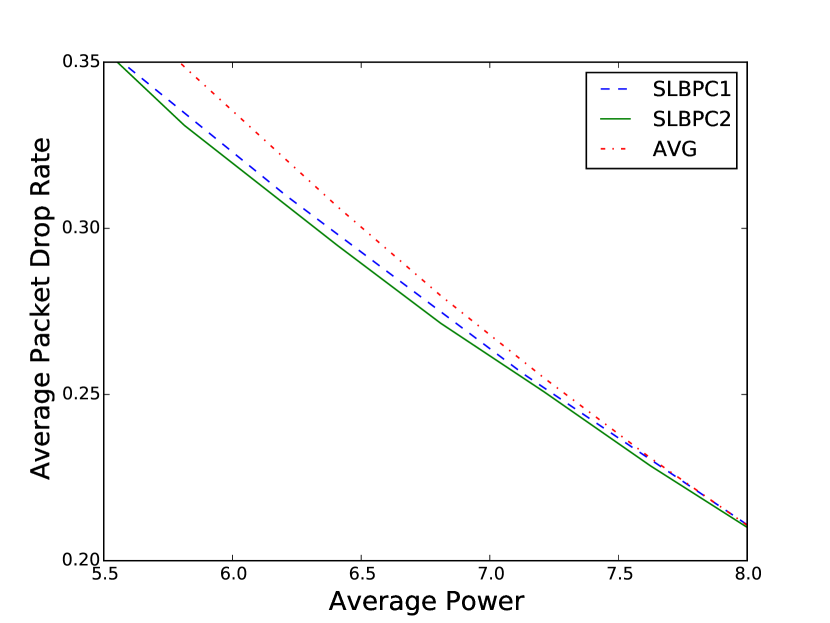
(a) Packet Drop Rate vs. Power

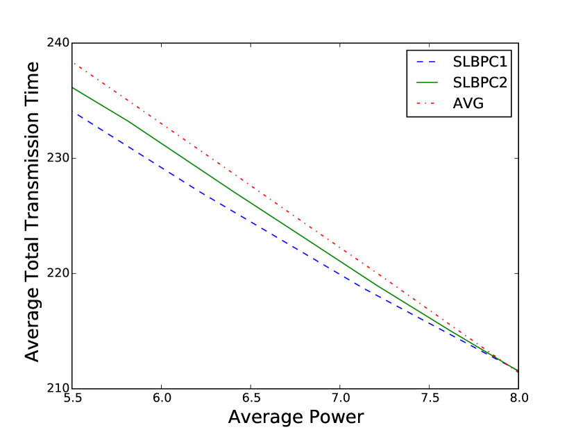
(b) Total Transmission Time vs. Power

Figure 7: Trade-off curves comparing SLBPC1, SLBPC2, and AVG.

We see that for a given power level, SLBPC1 achieves a lower packet drop rate than AVG and that SLBPC2 achieves a lower packet drop rate than SLBPC1. The advantage of the SLBPC algorithms over AVG is most apparent in the low power regime. This demonstrates that the SLBPC algorithms enable a higher fidelity packet stream with less power used. The SLBPC algorithms also reduce the total amount of transmission time. However, it is interesting to note that SLBPC1 is better at reducing the total transmission time than SLBPC2 is. Recall that SLBPC1 is a function only of the backlog so SLBPC1 makes reducing backlog pressure the primary objective. Since backlog pressure is a proxy for total delay, this behavior is expected.

6 Conclusions

This paper examines the problem of transmitting packets across a stochastically fluctuating wireless link while balancing power usage, overall latency, and jitter constraints. By considering a special case of the optimal transmitter power control problem, we have developed mathematically justified heuristics that are useful when designing sub-optimal power control schemes. In particular, we have analytically characterized how the optimal power control should vary with the backlog and how the optimal power control should react to approaching deadlines. By incorporating these structural properties into the Sublinear-Backlog Power Control (SLBPC) scheme, we have demonstrated how our theoretical results can be leveraged to build low-complexity approximations of the optimal power control. Monte Carlo simulations show that the SLBPC scheme is a good approximation for the optimal power control scheme. An additional simulations show that SLBPC outperforms benchmark algorithms in realistic settings.

References

References

- [1] H. Fattah, C. Leung, An overview of scheduling algorithms in wireless multimedia networks, IEEE Wireless Communications 9 (5) (2002) 76–83.
- [2] A. Dua, C. Chan, N. Bambos, J. Apostolopoulos, Channel, deadline, and distortion (CD2) aware scheduling for video streams over wireless, IEEE Transactions on Wireless Communications 9 (3) (2010) 1001–1011.
- [3] A. Asadi, Q. Wang, V. Mancuso, A survey on device-to-device communication in cellular networks, IEEE Communications Surveys Tutorials (99).
- [4] M. Zulhasnine, C. Huang, A. Srinivasan, Efficient resource allocation for device-to-device communication underlaying LTE network, in: IEEE International Conference on Wireless and Mobile Computing, Networking and Communications, 2010, pp. 368–375.
- [5] D. Camps-Mur, A. Garcia-Saavedra, P. Serrano, Device-to-device communications with Wi-Fi Direct: overview and experimentation, IEEE Wireless Communications 20 (3) (2013) 96–104.
- [6] Y. Li, A. Markopoulou, N. Bambos, J. Apostolopoulos, Joint power-playout control for media streaming over wireless links, IEEE Transactions on Multimedia 8 (4) (2006) 830–843.
- [7] B. Xing, K. Seada, N. Venkatasubramanian, An Experimental Study on Wi-Fi Ad-Hoc Mode for Mobile Device-to-Device Video Delivery, in: IEEE INFOCOM Workshops 2009, 2009, pp. 1–6.
- [8] IEEE 802.11 Working Group, Wireless LAN medium access control (MAC) and physical layer (PHY) specifications.
- [9] M. Chiang, P. Hande, T. Lan, C. W. Tan, Power control in wireless cellular networks, Foundations and Trends® in Networking 2 (4) (2008) 381–533.
- [10] L. B. Le, Fair resource allocation for device-to-device communications in wireless cellular networks, in: IEEE Global Communications Conference, 2012, pp. 5451–5456.
- [11] C.-H. Yu, K. Doppler, C. Ribeiro, O. Tirkkonen, Resource sharing optimization for device-to-device communication underlaying cellular networks, IEEE Transactions on Wireless Communications 10 (8) (2011) 2752–2763.
- [12] S. Kandukuri, S. Boyd, Optimal power control in interference-limited fading wireless channels with outage-probability specifications, IEEE Transactions on Wireless Communications 1 (1) (2002) 46–55.
- [13] D. O. Neill, A. J. Goldsmith, S. Boyd, Optimizing adaptive modulation in wireless networks via utility maximization, in: IEEE International Conference on Communications, IEEE, 2008, pp. 3372–3377.
- [14] M. J. Neely, Delay-based network utility maximization, IEEE/ACM Transactions on Networking 21 (1) (2013) 41–54.
- [15] M. J. Neely, Optimal energy and delay tradeoffs for multiuser wireless downlinks, IEEE Transactions on Information Theory 53 (9) (2007) 3095–3113.
- [16] J.-H. Kim, K.-Y. Chwa, Scheduling broadcasts with deadlines, Theoretical Computer Science 325 (3) (2004) 479–488.
- [17] N. T. Argon, S. Ziya, R. Righter, Scheduling impatient jobs in a clearing system with insights on patient triage in mass casualty incidents, Probability in the Engineering and Informational Sciences 22 (03) (2008) 301–332.
- [18] A. C. Dalal, S. Jordan, Optimal scheduling in a queue with differentiated impatient users, Performance Evaluation 59 (1) (2005) 73–84.
- [19] J. M. George, J. M. Harrison, Dynamic control of a queue with adjustable service rate, Operations Research 49 (5) (2001) 720–731.
- [20] N. Master, N. Bambos, Power control for wireless streaming with HOL packet deadlines, in: IEEE International Conference on Communications, IEEE, 2014, pp. 2263–2269.
- [21] N. Master, N. Bambos, Service rate control for jobs with decaying value, in: American Control Conference, IEEE, 2015, pp. 3255–3260.
- [22] E. N. Gilbert, Capacity of a burst-noise channel, Bell system technical journal 39 (5) (1960) 1253–1265.
- [23] H.-S. Wang, N. Moayeri, Finite-state Markov channel – a useful model for radio communication channels, IEEE Transactions on Vehicular Technology 44 (1) (1995) 163–171.
- [24] N. Bambos, S. Kandukuri, Power controlled multiple access (pcma) in wireless communication networks, in: Joint Conference of the IEEE Computer and Communications Societies (INFOCOM), Vol. 2, 2000, pp. 386–395.
- [25] D. Son, B. Krishnamachari, J. Heidemann, Experimental analysis of concurrent packet transmissions in wireless sensor networks, ACM SenSys, Boulder, USA.
- [26] J. Walrand, An introduction to queueing networks, Vol. 165, Prentice Hall Englewood Cliffs, NJ, 1988.
- [27] M. L. Puterman, Markov decision processes: discrete stochastic dynamic programming, John Wiley & Sons, 2009.
- [28] Ö. Alay, T. Korakis, Y. Wang, S. Panwar, An experimental study of packet loss and forward error correction in video multicast over ieee 802.11 b network, in: IEEE Consumer Communications and Networking Conference, IEEE, 2009, pp. 1–5.
- [29] A. Barron, J. Rissanen, B. Yu, The minimum description length principle in coding and modeling, IEEE Transactions on Information Theory 44 (6) (1998) 2743–2760.
- [30] D. M. Topkis, Minimizing a submodular function on a lattice, Operations research 26 (2) (1978) 305–321.
- [31] R. F. Serfozo, Monotone optimal policies for markov decision processes, in: Stochastic Systems: Modeling, Identification and Optimization, II, Springer, 1976, pp. 202–215.
- [32] M. H. Veatch, L. M. Wein, Monotone control of queueing networks, Queueing Systems 12 (3-4) (1992) 391–408.
- [33] A. Dragut, Structured optimal policies for markov decision processes: lattice programming techniques, Wiley Encyclopedia of Operations Research and Management Science.
- [34] R. L. Cruz, A. V. Santhanam, Optimal routing, link scheduling and power control in multihop wireless networks, in: Joint Conference of the IEEE Computer and Communications Societies (INFOCOM), Vol. 1, IEEE, 2003, pp. 702–711.
- [35] M. Goyal, A. Kumar, V. Sharma, Power constrained and delay optimal policies for scheduling transmission over a fading channel, in: Joint Conference of the IEEE Computer and Communications Societies (INFOCOM), Vol. 1, IEEE, 2003, pp. 311–320.
- [36] I. Bettesh, S. Shamai, Optimal power and rate control for minimal average delay: The single-user case, IEEE Transactions on Information Theory 52 (9) (2006) 4115–4141.
- [37] T. H. Cormen, C. E. Leiserson, R. L. Rivest, C. Stein, et al., Introduction to algorithms, MIT press Cambridge, 2001.
- [38] S. Boyd, L. Vandenberghe, Convex optimization, Cambridge university press, 2004.