Pulse-noise approach for classical spin systems

Abstract

For systems of classical spins interacting with the bath via damping and thermal noise, the approach is suggested to replace the white noise by a pulse noise acting at regular time intervals $\Delta t$, within which the system evolves conservatively. The method is working well in the typical case of a small dimensionless damping constant $\lambda$ and allows a considerable speed-up of computations by using high-order numerical integrators with a large time step $\delta t$ (up to a fraction of the precession period), while keeping $\delta t\ll\Delta t$ to reduce the relative contribution of noise-related operations. In cases when precession can be discarded, $\delta t$ can be increased up to a fraction of the relaxation time $\propto 1/\lambda$ that leads to a further speed-up. This makes equilibration speed comparable with that of Metropolis Monte Carlo. The pulse-noise approach is tested on single-spin and multi-spin models.

I Introduction

Systems of localized spins on a lattice, considered classically as vectors $\mathbf{s}$ of unit length, are receiving an increasing interest because of their application in computer simulations of magnetic materials. Although this classical model misses the exact form of the low-temperature magnetization formed by quantum effects (e.g., the Bloch law for ferromagnets), it provides a good overall description of magnetic properties, including non-uniform states. Atomistic models of classical spins are working at any temperature and overall explain thermal properties including phase transitions. In this respect they are superior to micromagnetics – a macroscopic approach in which thermal properties have to be taken from experiment.

The temperature in atomistic classical spin systems can be fixed by their interaction with the environment modeled by the damping term introduced by Landau and Lifshitz Landau and Lifshitz (1935) plus white-noise-type random fields $\boldsymbol{\zeta}$ known as Langevin sources and introduced by Brown W. F. Brown (1963). This equation has the form

$$\mathbf{\dot{s}}=\gamma\left[\mathbf{s}\times\left(\mathbf{H}_{\mathrm{eff}}+\boldsymbol{\zeta}\right)\right]-\gamma\lambda\left[\mathbf{s}\times\left[\mathbf{s}\times\mathbf{H}_{\mathrm{eff}}\right]\right],$$ (1)

where $\mathbf{H}_{\mathrm{eff}}$ is the effective magnetic field, $\gamma$ is gyromagnetic ratio, and $\lambda$ is the dimensionless damping constant. Such a stochastic model is equivalent to the Fokker-Planck equation, as was shown by Brown for superparamagnetic particles. The equilibrium solution of the Fokker-Planck equation should be Boltzmann distribution, that requires a relation between damping and noise,

$$\left\langle\zeta_{\alpha}(t)\zeta_{\beta}(t^{\prime})\right\rangle=\frac{2\lambda T}{\gamma\mu_{0}}\delta_{\alpha\beta}\delta(t-t^{\prime}).$$ (2)

Here $\mu_{0}$ is the magnetic moment of one atom and $k_{B}=1$. Microscopic theories always suggest $\lambda\ll 1$.

It was shown that the vector product in the noise term dictates the double-vector product form of the Landau-Lifshitz damping term Garanin et al. (1990). For instance, in the case of noise being anisotropic, the damping term has to be accordingly modified. Moreover, the main source of thermal agitation of spins, lattice vibrations, does not produce fluctuating fields. There are rather fluctuations of the crystal-field anisotropy tensor. This leads to a more complicated model of noise Garanin et al. (1990) that was not explored, however. The model above, although physically questionable, is the simplest possible model and it does not lead to visible inconsistencies.

For many-spin systems, the Fokker-Planck equation becomes a numerically intractable partial differential equation for the joint probability density of orientations of all spins. On the other hand, the system of ordinary differential equations (ODE) of the many-spin stochastic model can be solved on modern computers in a relatively straighforward way. Early implementations were done for superparamangetic particles Lyberatos and Chantrell (1993); García-Palacios and Lázaro (1998). Later the method was applied to magnetic particles considered as many-spin systems Chubykalo et al. (2002); Chubykalo-Fesenko et al. (2006); Suh et al. (2008); Bastardis et al. (2012). A recent review of the method for magnetic materials provides a link to a software package developed by authors Evans et al. (2014). In particular, the Landau-Lifshitz-Langevin (LLL) method reproduces the same temperature dependence of the magnetization of the Heisenberg model, as Metropolis Monte Carlo.

Currently most of stochastic-dynamics routines for classical spin systems are using rather primitive Heun method having a quadratic accuracy in integration steps, the latter being chosen small to avoid instabilities. For this reason, the computing speeds falls far behind the speed of the numerical solution of noisless spin models. Generating noise in these programs is taking longer time than solving equations of motion.

Fortunately, coupling to the environment $\lambda$ is typically small in spin systems, so that taking it into account should simplify. The idea of this work is to replace the white noise by a sequence of pulses equally spaced in time. In the underdamped case the interval of free evolution between noise pulses can be made comparable with the spin precession period or longer, if precession can be discarded, and within these intervals high-order ODE solvers can be used with a large integration step.

The main part of this paper is organized as follows. The proposed pulse-noise method is described in Sec. II. Sec. III is devoted to testing the method on one-spin problems, including thermally-activated escape. In Sec. IV the pulse-noise method is tested on many-spin systems and its speed is compared to that of Monte Carlo.

II The method

In all existing approaches, noise is considered as invariable within $n$th integration step $\varDelta t$ and equal to

$$\boldsymbol{\zeta}_{n}=\sqrt{\frac{2\lambda T}{\gamma\mu_{0}\varDelta t}}\mathbf{G}_{n}.$$ (3)

Here $\mathbf{G}_{n}$ is $n$th realization of a three-component vector, each component being a normal distribution with a unit dispersion. Such approximated noise will be called rectangular noise. The coefficient here is fixed by the sum rule

$$\intop_{-\infty}^{\infty}dt\left\langle\zeta_{\alpha}(t)\zeta_{\beta}(t^{\prime})\right\rangle=\varDelta t\sum_{n}\left\langle\zeta_{n\alpha}\zeta_{n^{\prime}\beta}\right\rangle=\frac{2\lambda T}{\gamma\mu_{0}}\delta_{\alpha\beta},$$ (4)

since $\left\langle G_{n\alpha}G_{n^{\prime}\beta}\right\rangle=\delta_{nn^{\prime}}\delta_{\alpha\beta}$.

The usual argument says that invariance of the noise within the integration step excludes high-order integration methods splitting the step into several substeps. In this case one has to generate the noise at the intermediate positions as well, causing a bigger amount of number crunching. However, since high-order methods require smoothness of derivatives, they would not work in this case anyway. Nevertheless, as soon as the rectangular-noise model is already adopted, it is quite reasonable to solve it with high-order integration methods that are more accurate and more stable. Below it will be shown that it makes a considerable positive effect.

The numerical efficiency can be drastically improved by replacing the rectangular noise by the pulse noise acting only at the boundaries of intervals $\varDelta t$. The latter can be taken large in the case of small damping, $\lambda\ll 1$. The action of each pulse is instantaneous rotation of the spin by the angle

$$\boldsymbol{\varphi}_{n}=\sqrt{\varLambda_{N}\varDelta t}\mathbf{G}_{n},$$ (5)

where $\varLambda_{N}\equiv 2\gamma\lambda T/\mu_{0}$ is the so-called Néel attempt frequency Garanin (1997). With $\boldsymbol{\varphi}=\varphi\mathbf{n}$ and $|\mathbf{n}|=1$ the rotation formula reads

$$\mathbf{s}^{\prime}=\mathbf{s}\cos\varphi+\left(\mathbf{n}\times\mathbf{s}\right)\sin\varphi+\mathbf{n}\left(\mathbf{s\bullet n}\right)\left(1-\cos\varphi\right).$$ (6)

Such a rotation would occur within the time interval $\varDelta t$ if nothing else than noise acted on the spin. Then, within the intervals $\varDelta t$, evolution of the noiseless system can be obtained by an efficient ODE solver making large steps $\delta t$ satisfying $\delta t<\varDelta t$. The value of $\delta t$ should be chosen so that noiseless dynamics (mainly precession of spins) be reproduced correctly. On the other hand, $\varDelta t$ should be a fraction of the relaxation time due to spin-bath interaction. In the underdamped case one can choose $\delta t\ll\varDelta t$, drastically reducing the computer time needed to generate the noise. In this case noisy dynamics becomes close to the noiseless dynamics, and it is only slightly modified by random kicks on the spins.

Separating simultaneous dynamics of the system under the influence of the noise and everything else into separate motions can be justified with the help of the Suzuki-Trotter expansion of exponential operators. The evolution of the system on the time interval $\varDelta t$ can be represented via the evolution operator $\hat{U}=e^{\hat{A}+\hat{B}}$, where $\hat{A}$ is due to noiseless dynamics and $\hat{B}$ is due to noise. Both of these operators depend on $\varDelta t$. In the underdamped case, if $\varDelta t$ is not too long, $\hat{B}$ becomes small even if $\hat{A}$ is not. Then one can use the second-order Suzuki-Trotter formula (see, e.g., Ref. Hatano and Suzuki (2005))

$$e^{\hat{A}+\hat{B}}\cong e^{\hat{A}/2}e^{\hat{B}}e^{\hat{A}/2}$$ (7)

that describes the sequence of (i) noiseless evolution during the interval $0.5\varDelta t$; (ii) rotation by the noise angle $\boldsymbol{\varphi}$, Eq. (6); (iii) repetition of (i). The a priori applicability condition of the pulse-noise approach is

$$\varphi\sim\sqrt{\varLambda_{N}\varDelta t}\ll 1.$$ (8)

One can see that the weaker is the damping $\lambda$ and the lower is the temperature, the longer noiseless interval $\varDelta t$ can be used. It does not make sense to expand Eq. (6) to the linear order in $\varphi$ since the spin length has to be conserved. There is another applicability condition, however. Non-thermal relaxation of the system during the time $\varDelta t$ should be small,

$$\gamma\lambda H_{\mathrm{eff}}\Delta t\ll 1.$$ (9)

In the opposite case the system will spend most of the time near its ground state and the averages will correspond to $T=0$.

All problems described by Eq. (1) fall into two categories: 1) Precession term $\gamma\left[\mathbf{s}\times\mathbf{H}_{\mathrm{eff}}\right]$ is important and has to be kept; 2) Precession term can be discarded.

The first (precessional) case is a regular situation in which using the pulse-noise model brings a huge computing speed-up in the typical underdamped case, $\lambda\ll 1$. Accurate numerical integration of the precession imposes the condition $\gamma H_{\mathrm{eff}}\delta t\ll 1$, where $\delta t$ is the integration step used by the ODE solver. For instance, a good ODE solver provides an acceptable accuracy for $\gamma H_{\mathrm{eff}}\delta t$ about 0.2 and even 0.25. In this case, one can use $\Delta t\gg\delta t$ and still satisfy Eqs. (8) and (9). As the result, the main computer time is being spent on solving the noiseless dynamics, while the time spent on computing rare noise kicks becomes negligible. This is true both for one-spin and many-spin systems.

The second (non-precessional) case is realized if one is interested in the averages of physical quantities at equilibrium. Since precession terms do not affect the equilibrium solution of the Fokker-Planck equation, they can be dropped. If the system has integrals of motion such as projection the total spin $\mathbf{S}$ on the symmetry axis $z$ in the case of uniaxial anisotropy, then even the dynamical behavior of $m_{z}\equiv\left\langle s_{z}\right\rangle$, not only its asymptotic value, becomes unaffected by the precession. In these cases one can discard the precession and use the resulting slow equation that can be numerically solved with a much larger integration step satisfying $\gamma\lambda H_{\mathrm{eff}}\delta t\ll 1$. This leads to an additional speed-up in comparison to the precessional case.

Within the standard method using continuous noise, dropping the regular precession term in the equation of motion leads only to a marginal improvement since there is still the noisy precession term that cannot be discarded. To the contrast, in the pulse-noise model precession term can be dropped entierely since precession due to the noise is accounted for by Eq. (6).

In the sequel, testing the pulse-noise approach will be done for different models. For the sake of transparency, instead of introducing different reduced quantities, some parameters and constants, such as $\gamma$, $\mu_{0}$, etc., will be set to 1. This should be taken into account in reading plots.

Details of the numerical implementation using Wolfram Mathematica are given in the Appendix.

III Testing the method on one-spin problems

III.1 Spin in a magnetic field

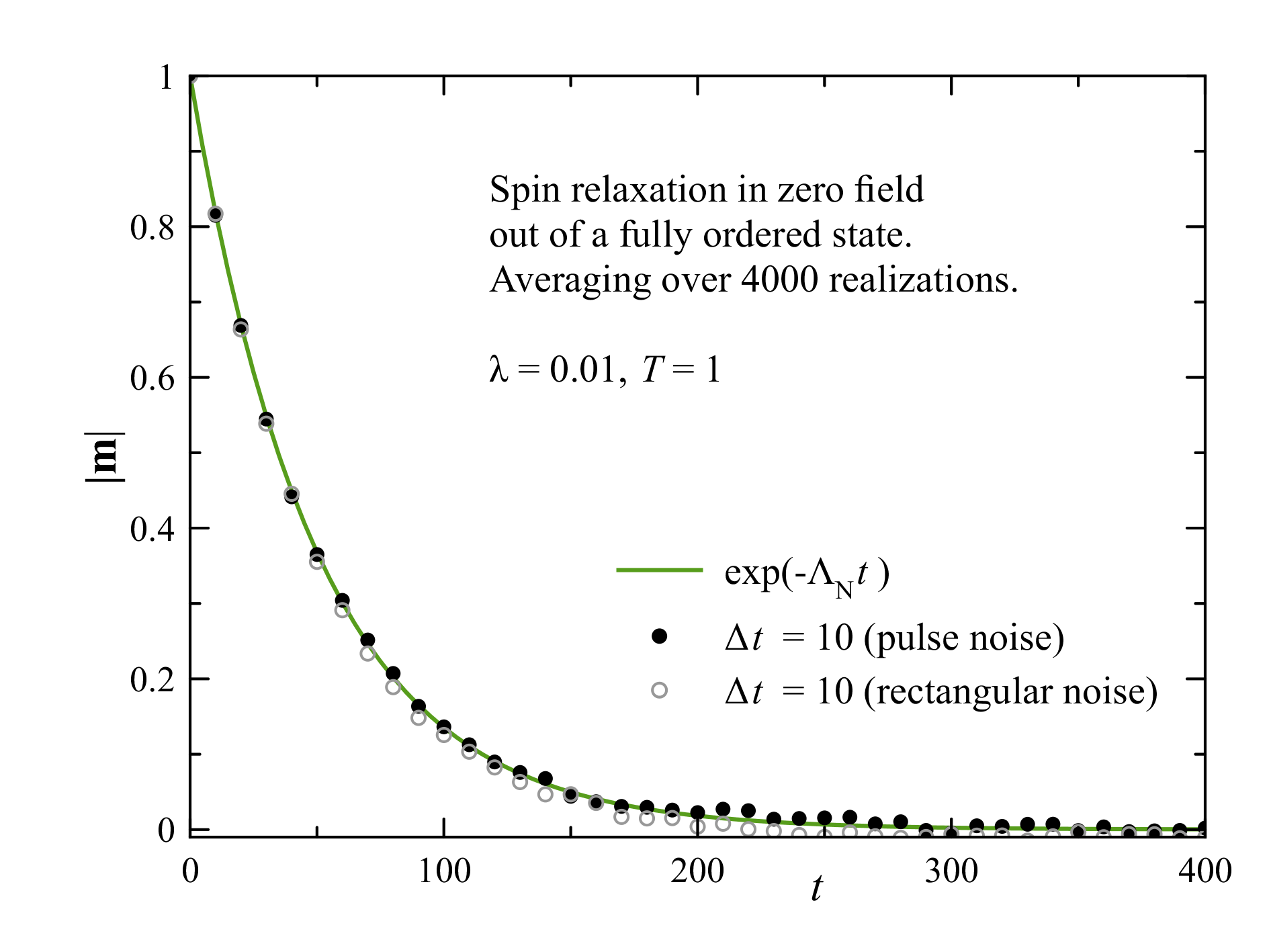
Figure 1: Exponential decay of the magnetization out of a completely ordered state under the action of the noise only (the high-temperature limit). The pulse-noise and rectangular-noise models yield the same results.

The first test to make is the test of the discretization of the noise into intervals $\varDelta t$ for the trivial system in which only the noise is present, that physically corresponds to high temperatures. In this case the Fokker-Planck equation for one spin readily yields the evolution of the magnetization $\mathbf{m}=\left\langle\mathbf{s}\right\rangle$ in the form

$$\mathbf{m}=\mathbf{m}_{0}e^{-\varLambda_{N}t}.$$ (10)

Fig. 1 shows this dependence together with the results of numerical solutions of the pulse-noise and rectangular-noise models with $\delta t=0.25$ and discretization time $\Delta t=10$ for $\lambda=0.01$, $T=1$. Here the RMS value of the rotation angle $\varphi_{\mathrm{RMS}}=\sqrt{\varLambda_{N}\varDelta t}\simeq 0.45$ is not small, still the pulse-noise model well reproduces the analytical result. The model with rectangular noise yields the same result that is not surprising. Whereas in the pulse-noise model rotations are instantaneous in the middle of the $\Delta t$ interval, in the rectangular-noise model they are performed gradually by the ODE solver to the same effect.

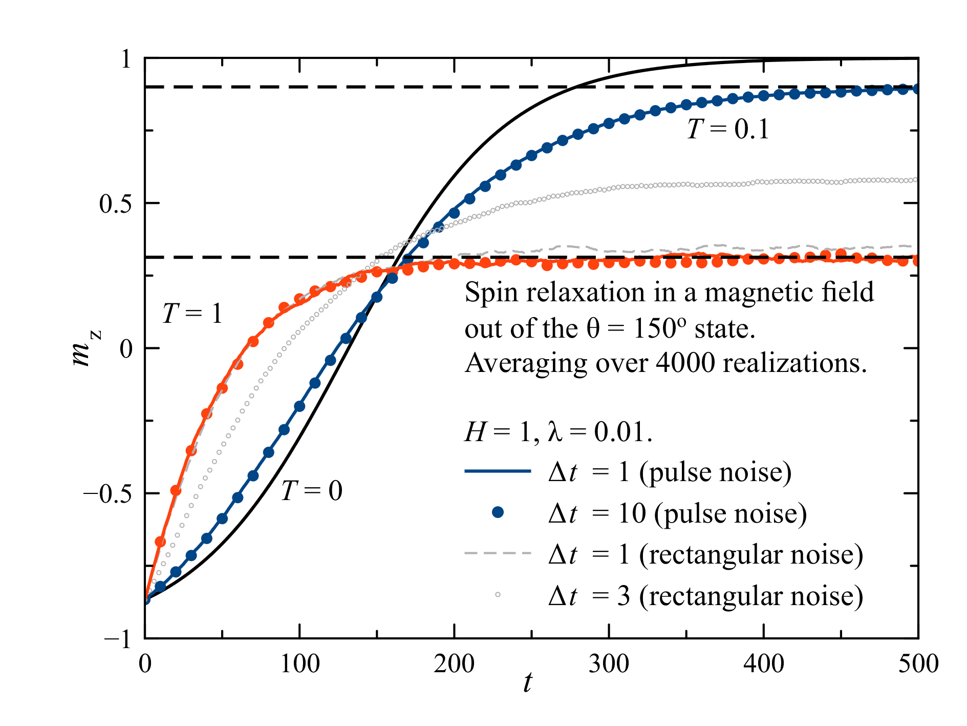
Figure 2: Relaxation of the spin in a magnetic field out of the completely ordered state directed at $\theta=150\textdegree$ to the field, at different temperatures and $\varDelta t$. Pulse-noise model works perfectly for $\Delta t=1$ (red, blue, and black lines) and holds up to $\Delta t=10$ (red and blue points), while the rectangular-noise model (gray) fails already at $\Delta t=3$.

For non-trivial spin Hamiltonians, starting with the spin in a magnetic field, the difference between the two noise models becomes tremendous. This can be seen in Fig. 2, where initially the spin is directed at $\theta=150^{\circ}$ to the field. Whereas the pulse-noise model yields visually the same results for $m_{z}(t)$ for $\Delta t=1$ and 10 (both with $\lambda=0.01$ and $H=1$) and asymptotically approaches the correct equilibrium value, the rectangular-noise model for $T=1$ is working only for $\Delta t=1$, although there a visible overestimation of $m_{z}(\infty)$. Already for $\Delta t=3$ this model breaks down completely, mimicking a significantly lower temperature. This can be interpreted as the rectangular noise being correlated and thus gentle, only slightly modifying the field instead of really kicking the spin. Here in all cases RK5 ODE solver with the integration time step $\delta t=0.25$ was used. For the sake of comparison, precession term was kept in the equation of motion, since for the rectangular-noise model it cannot be discarded.

The spin-in-a-field model is convenient for making a comparison with the standard stochastic-dynamics approach using the Heun ODE solver. It was found that for $T=1$ and other parameters as indicated above, the Heun solver is stable for $\delta t\leq 0.04$, where it yields visibly same results as the pulse-noise method in Fig. 2. Above this value the Heun method crashes even if the spin length is constantly corrected. Ref. Evans et al. (2014) uses natural units with $J=3\times 10^{-21}$ J/link for magnetic particles. The time step was $\delta t_{\mathrm{natural}}=10^{-15}$s but it had to be decreased to $10^{-16}$s near the Curie point. In dimensionless units used here, $10^{-15}$s corresponds to $\delta t=\left(J/\hbar\right)\delta t_{\mathrm{natural}}\simeq 0.03$. Other authors also report using rather small time steps with the Heun method, that makes it slow. Within the Heun method in the present implementation, most of the computer time is being spent on generation of random numbers, and the resulting computing speed is 10 times lower than that of the pulse-noise method using RK5 solver with $\delta t=0.25$ and $\Delta t=10$.

Even within the rectangular-noise model, using the more stable RK5 instead of the Heun method allows to use $\delta t=0.25$ to reach a speed-up by a factor of 4. This confirms the statement about usefulness of high-order integration methods made at the beginning of Sec. II.

Fig. 3 shows one realization of the spin precession with relaxation in a magnetic field in the presence of a pulse noise for $H=1$, $T=0.01$, $\lambda=0.04$. Here the computation was done with $\delta t=0.25$ and $\varDelta t=\delta t$. One can see precession with relaxation terminating in a noisy behavior.

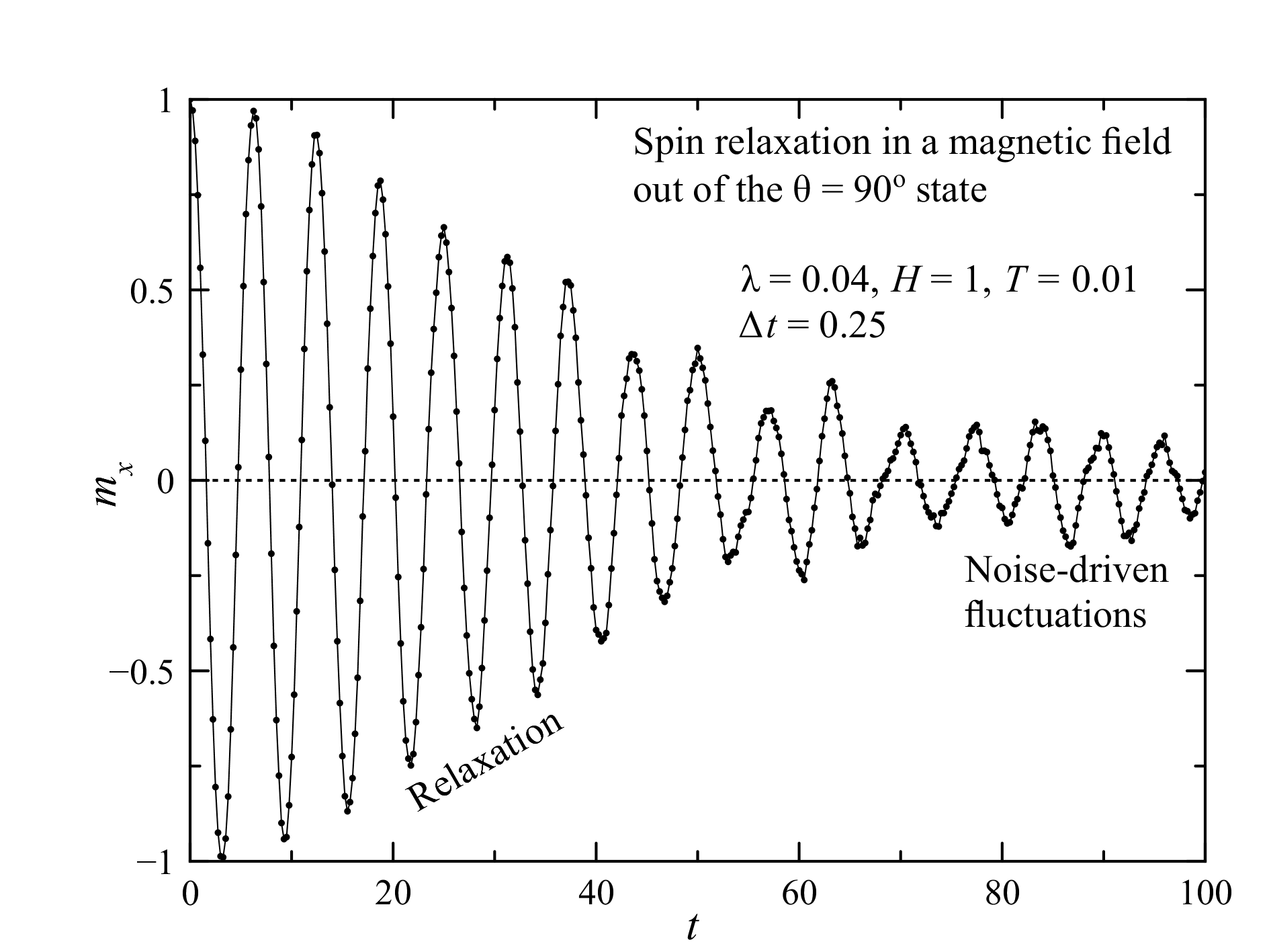
Figure 3: One realization of the spin precession with relaxation in the presence of a pulse noise. The initial direction of the spin is perpendicular to the field. For the temperature as low as $T=0.01,$ there is a regime of nearly-deterministic relaxation terminating in the regime of noise-driven fluctuations.

Note that noiseless precession and relaxation of a spin in a magnetic field can be described analytically, so that there is no need of numerical integration. Transformation of $s_{z}$ and the transverse spin component $s_{\bot}=\sqrt{s_{x}^{2}+s_{y}^{2}}$ during the time interval $\Delta t$ is described by Chudnovsky and Garanin (2002)

$$s_{z}^{\prime} = \frac{\sinh\left(\tau\right)+s_{z}\cosh\left(\tau\right)}{\cosh\left(\tau\right)+s_{z}\sinh\left(\tau\right)}$$

$$s_{\bot}^{\prime} = \sqrt{1-s_{z}^{\prime 2}},\qquad\tau\equiv\gamma\lambda H\Delta t.$$ (11)

Here one can trivially add precession to find the values of $s_{x}$ and $s_{y}$. Thus evolution of the spin in a field within the pulse-noise model is a map combined of discrete transformations of two kinds. Same is true for the rectangular-noise model, although working out analytics is more cumbersome because of changing the direction of the total field. Although the transformation above is exact, $\tau$ has to be small because of Eq. (9).

Let us now investigate the a posteriori accuracy of the pulse-noise approximation by looking at the equilibrium value of $m_{z}$ obtained by extensive averaging for the spin-in-a-field model using Eqs. (6) and (11). After an initial thermalization period, spin evolution was monitored within the time interval $t_{\max}=10^{6}$, and $m_{z}=\left\langle s_{z}\right\rangle$ was computed by averaging the values at the end of each time interval $\Delta t$. Such computations were run in parallel cycles, using three different computers having 4, 8, and 16 cores. The final computed average corresponds to the total averaging time $t_{\mathrm{avr}}=t_{\max}\times N_{\mathrm{cores}}\times N_{\mathrm{cycles}}$.

Fig. 4 shows the dependence of $m_{z}$ computed with $t_{\mathrm{avr}}\simeq 2\times 10^{9}$, as explained above, on $\Delta t$ for $H=1$ and $\lambda=0.01$. At the elevated temperature $T=1$ (Fig. 4a), the deviation from the exact result goes down almost linearly with some upward curwature. This upward curvature is dominating at the low temperature $T=0.1$ in Fig. 4b, so that the deviation from the exact result is positive. This can be explained by the effect commented upon below Eq. (9), since here $\gamma\lambda H\Delta t=1$ at $\Delta t=100$. However, the effect is smaller than expected, thus the applicability condition in Eq. (9) is somewhet less stringent than it seems. The scales of $\Delta t$ in both computations were chosen so that the range of $\varLambda_{N}\Delta t$ is the same, as shown in top $x$ axes. In both cases $\varLambda_{N}\Delta t=0.1$ provides an accuracy good enough, as shown in the figures, and it satisfies the thermal applicability condition, Eq.$\,(\ref{eq:phi_condition}).$ Note that low temperatures are more favorable for the pulse-noise model: $\varLambda_{N}\Delta t=0.1$ corresponds to $\Delta t=5$ for $T=1$ and $\Delta t=50$ for $T=0.1$. In the plots, $\varDelta m_{z}$ is the deviation from the exact value of $m_{z}$, that for $\varLambda_{N}\Delta t=0.1$ has different signs for $T=1$ and $T=0.1$.

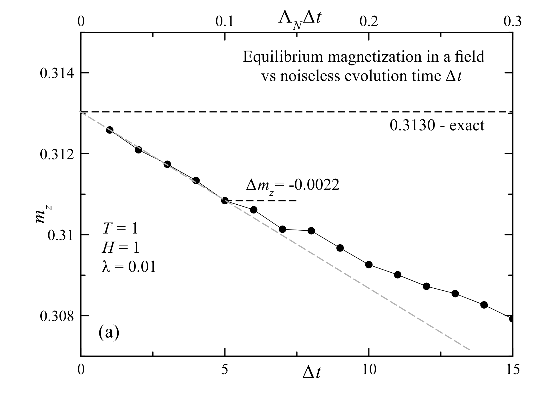
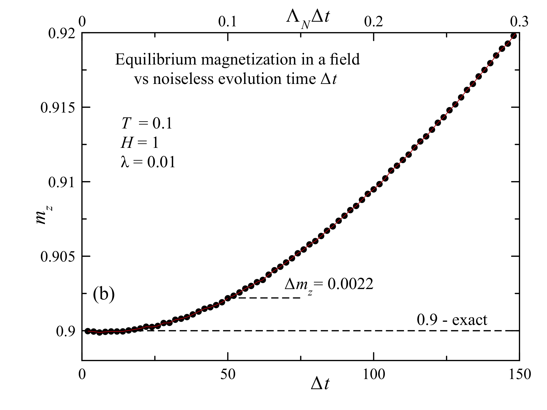
Figure 4: Equilibrium magnetization $m_{z}$ for the spin-in-a-field model vs noiseless evolution time $\Delta t$ (bottom $x$ axes) and parameter $\varLambda_{N}\Delta t$ (top $x$ axes) for $H=1$ and $\lambda=0.01$. The curves begin from the exact values of $m_{z}$ on the left, and the error of the pulse-noise approximation increases with $\varDelta t$. (a) $T=1$; (b) $T=0.1.$

III.2 Thermally activated escape rate of a uniaxial spin in a transverse field

Uniaxial spin in a transverse field is an example of a system, for which precession is relevant in the dynamics. The energy

$$\mathcal{H}=-Ds_{z}^{2}-Hs_{x}$$ (12)

for $h\equiv H/(2D)<1$ possesses two degenerate minima at the angle $\theta=\arcsin h$ to $z$ axis. The saddle point is $\mathbf{s}=(1,0,0)$ and the energy barrier between the minima is given by $\Delta U=D(1-h)^{2}$. In the case of a well-developed saddle, the thermally activated escape rate over the barrier $\Gamma$ reads Garanin et al. (1999)

$$\Gamma=\frac{\omega_{0}}{2\pi}Ae^{-\sigma(1-h)^{2}},$$ (13)

where $\sigma\equiv D/T$ and $\omega_{0}=2\gamma D\sqrt{1-h^{2}}$ is the frequency of the ferromagnetic resonance near the bottom of the well, so that $\omega_{0}/(2\pi)$ can be interpereted as the attempt frequency. The factor $A$ has different forms in the high-damping (HD), intermediate damping (ID) and low damping (LD) regimes, similarly to the problem of a particle in a potential well considered by Kramers Kramers (1940). Crossovers between these regimes and those to the uniaxial case have been studied in Ref. Garanin et al. (1999). In the HD regime, $\lambda\gtrsim 1$, one has $A\propto\lambda$ (or $A\propto 1/\lambda$ if the Gilbert equation is used). Since HD regime is untypical for spin systems, it will not be considered here. In the ID regime $\lambda\lesssim 1$ that corresponds to the transition-state theory, one has $A=1$. Finally, in the LD case the energy dissipated over the separatrix trajectory around one well becomes smaller than thermal energy, $\delta E\sim\lambda D\lesssim T$, and the energy-diffusion regime sets in. In this case one has $A=\delta E/(2T)$ that can be written in the form

$$A\equiv A^{(LD)}=\lambda\sigma F(h),$$ (14)

where

$$F(h)=\frac{1}{2}\oint_{f=f_{c}}\left[(1-x^{2})\frac{\partial f}{\partial x}d\phi-\frac{1}{1-x^{2}}\frac{\partial f}{\partial\phi}dx\right],$$ (15)

$x\equiv\cos\theta$, and $f$ is the dimensionless energy in the spherical coordinates,

$$f(x,\phi)=-\mathcal{H}/D=x^{2}+2h\sqrt{1-x^{2}}\cos\phi,$$ (16)

$f_{c}=2h$. The maximal value of $x$ on the separatrix is given by $x_{c}=2\sqrt{h(1-h)}$. It is convenient to calculate $F(h)$ as the integral over $x$ over the half of the separatrix between 0 and $x_{c}$, with $\phi=0$ at both points. After some algebra one obtains

$$F(h)=\intop_{0}^{1}\frac{x_{c}du}{1-x_{c}^{2}u^{2}}\left[\frac{u\left[2(1-h)-x_{c}^{2}u^{2}\right]^{2}}{\sqrt{1-u^{2}}}+x_{c}\sqrt{1-u^{2}}\right]$$ (17)

that can be computed numerically, see Fig. 5. For $h\ll 1$ this simplifies to $F(h)=8\sqrt{h}$ Klik and Gunther (1990); Garanin et al. (1999).

Non-trivial crossover between the ID and LD regimes is given by the Melnikov’s formula Mel’nikov (1985); Mel’nikov and Meshkov (1986); Coffey et al. (2001). However, for the current purposes (plotting the escape rate in a log scale) it is sufficient to use the interpolation

$$A=A^{(ILD)}=\frac{A^{(LD)}}{1+A^{(LD)}}.$$ (18)

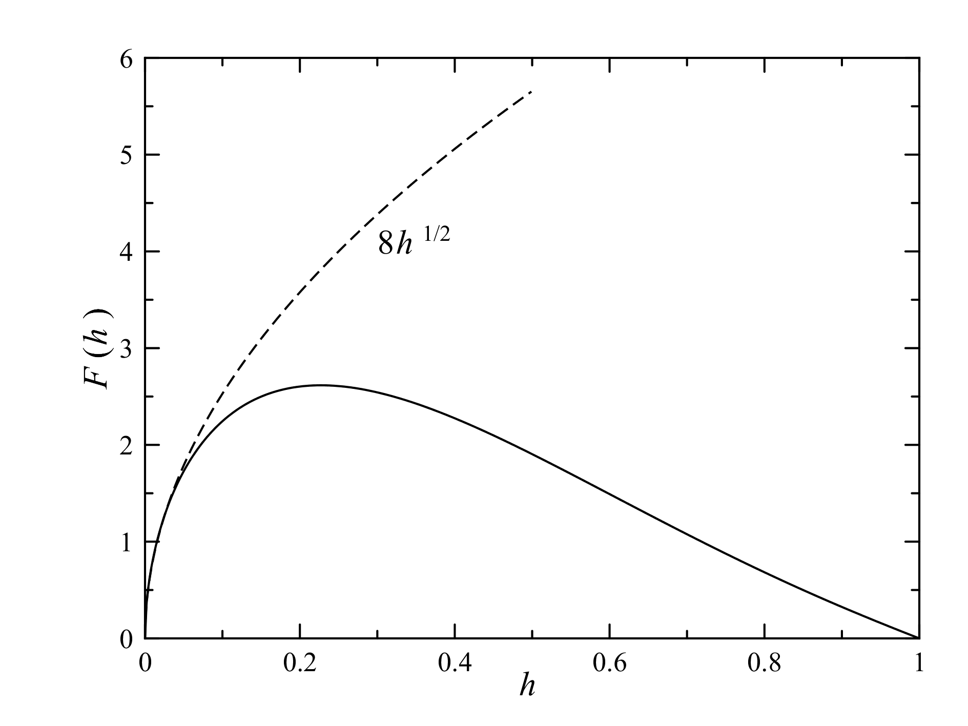
Figure 5: Function $F(h)$ in the low-damping escape rate of a uniaxial spin in a transverse field, Eq. (14).

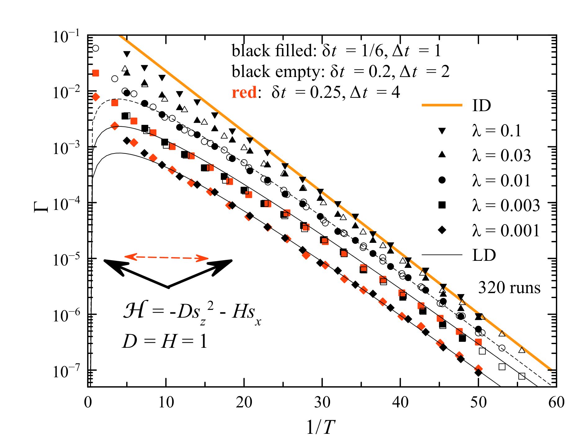
Figure 6: Temperature dependence of the thermal activation escape rate of a uniaxial spin in a transverse field for different values of damping $\lambda$, obtained with different values of the parameters in the pulse-noise approximation. The ID line corresponds to $A=1$ in Eq. (13). The LD lines use Eq. (14) with $F(h)=1.90$ for $h=1/2$. The dashed line uses the LD-ID interpolation, Eq. (18).

This problem has been investigated by different methods (see, e.g., Ref. Kalmykov et al. (2010) and references therein). The results of numerical calculation of the escape rate using Eq. (1) with the pulse-noise approximation with different parameters are shown in Fig. 6 together with analytical results with which they fully agree. In the computations, spins were initially put at the bottom of the potential well $\phi=0$, $\sin\theta=h$ with $h=1/2$ and then the evolution routine was run using Butcher’s RK5 ODE solver with time step $\delta t$ and random pulse rotations with noise-free evolution time $\Delta t$. By construction [see Eq. (7)] the ratio $\Delta t/\delta t$ has to be an even number. After crossing the line $s_{z}=0$ the computation was stopped and the first-passage time was recorded. For each temperature 320 runs were done in parallel, the mean first-passage time (MFPT) was computed and escape rate $\Gamma$ was found as its inverse. A similar procedure is being used in the experiment Coffey et al. (1998).

The results in Fig. 6 show that for $\lambda=0.1$ the ID regime, Eq. (13) with $A=1,$ is realized for most temperatures. On the other hand, the results for $\lambda=0.003$ and 0.001 are well described by the LD formula, Eq.$\,(\ref{eq:ALD})$. The cases $\lambda=0.03$ and 0.01 are ILD crossover cases. In particular, the $\lambda=0.01$ results are well described by the interpolation formula, Eq. (18).

Concerning the accuracy of computations, the set $\delta t=1/6$ and $\Delta t=1$ was used as the reference one as it provides accurate resuls for all dampings and temperatures studied here. Already for this set, the ratio $\Delta t/\delta t=6$ ensured that the computer time spent on generating random numbers and rotations of the spin is negligibly small in comparison to the time spent on solving the noiseless equation of motion. For higher values of damping, $\lambda=0.01$ and 0.03, the computation could be sped up by choosing $\delta t=0.2$ and $\Delta t=2$ with essentially the same results. However, for $\Delta t=4$ obtained values of $\Gamma$ were visibly too high. This can be explained by strong kicks allowing spins to cross the barrier at once from a position slightly below it, that results in effective reducing the barrier. For lower damping, such as $\lambda=0.001$ and 0.003, the set $\delta t=0.25$ and $\Delta t=4$ could be used without significant loss of accuracy, that allowed an even greater speed-up. Increasing integration step above $\delta t=0.25$ leads to a sharp decrease of accuracy and even to an instability. Thus the integration time step larger than 0.25 has to be avoided, if the full equation of motion including precession is used.

IV Pulse-noise approach for many-spin systems

Many-spin systems usually have their own non-trivial dynamics, only slightly modified by the coupling to the bath. Dynamic quantities such as relaxation rates are typically due to spin-spin interactions. The role of the coupling to the bath is merely to maintain the spin system at the preset temperature. Thus the coupling to the bath $\lambda$ can be chosen small, so that the noiseless evolution time $\Delta t$ in the pulse-noise model can be made long, while satisfying $\varLambda_{N}\Delta t=2\gamma\lambda T\Delta t\ll 1$. This reduces the fraction of the computer time used to generate random numbers to insignificant values, and the computation acquires the speed of those for isolated systems. Of course, one has to generate many random numbers for a good statistical averaging. In large systems it occurs automatically because of a large number of spins.

There are, however, special sutuations where coupling to the bath becomes more important (non-precessional case). This happens for simple spin systems having integrals of motion that are broken by the coupling to the bath (e.g., isotropic and uniaxial spin systems). In particular, the prefactor in the overbarrier thermal-activation rate of a magnetic particle with a uniaxial anisotropy is proportional to $\lambda$, while adding a transverse field or a transverse anisotropy breaks conservation of $S_{z}$ and makes the prefactor independent of $\lambda$ and much larger Garanin et al. (1999).

As time dependence of the integrals of motion is entirely due to spin-bath relaxation and noise, one can discard the fast motion (precession around the effective field) in Eq. (1). Resulting slow equation of motion can be solved with a much larger integration step $\delta t$, saving computer time ($\gamma\lambda H_{\mathrm{eff}}\delta t\ll 1$ instead of $\gamma H_{\mathrm{eff}}\delta t\ll 1$, that makes a big difference for weak damping $\lambda\ll 1$).

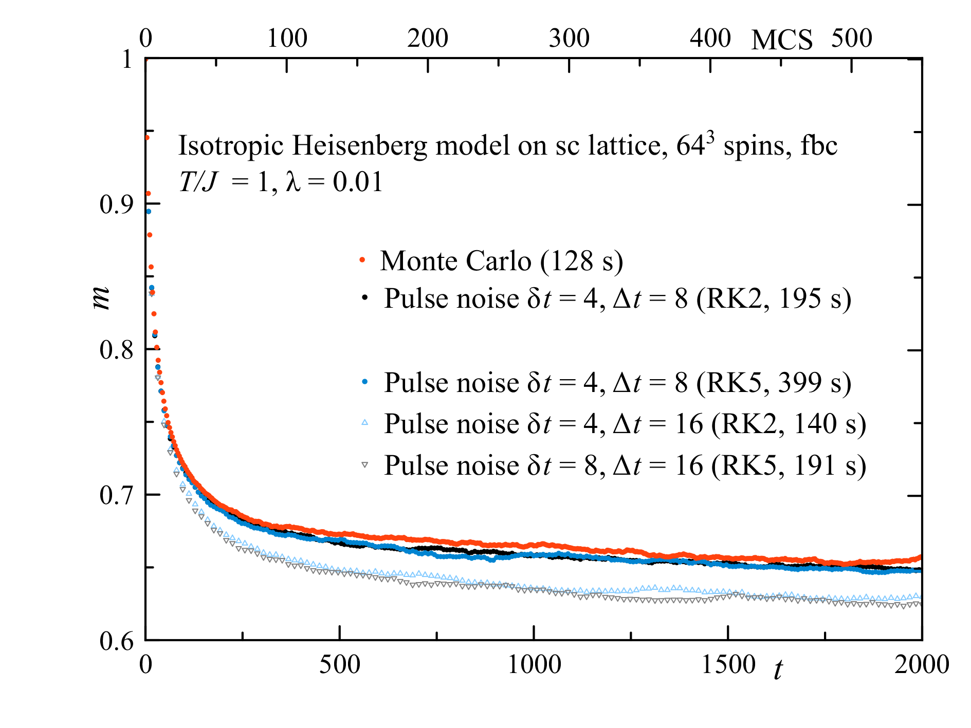
Figure 7: Monte Carlo vs pulse-noise approach: Relaxation of the magnetization of a $64\times 64\times 64$ particle with isotropic Heisenberg coupling and free boundary conditions out of a completely ordered state at $T/J=1$. Numerical methods and computing times are indicated in brackets.

Fig. 7 shows the magnetization relaxation out of a fully ordered state for a particle of $64^{3}=262144$ spins on a simple cubic lattice, coupled by the isotropic Heisenberg exchange $J$ with free boundary conditions at temperature $T/J=1$ that is below the Curie temperature $T/J=1.444$ in the bulk. The curves were obtained by variations of the pulse-noise method and by the standard Metropolis Monte Carlo method Metropolis et al. (1954), for a comparison. In the current implementation, one Monte Carlo step (MCS) includes a successive update of all spins in the system by adding a randomly directed vector $\mathbf{R}$ to each spin, and then normalizing the spin, and computing the energy change $\Delta E$. This trial is accepted unconditionally if $\Delta E<0$ and accepted with probability $e^{-\Delta E/T}$ if $\Delta E>0$. The length of $\mathbf{R}$ was chosen as $R=1.55\sqrt{T/(6J)}$ that yields about 50% acceptance rate in a wide temperature range. More details of the Monte Carlo method and more trial choices can be found in Ref. Nowak (2007). Note that for such large system sizes, most of fluctuations self-average and relaxation curves become pretty smooth without avegaring over runs. The figure shows the results of one run for each set of parameters. Both pulse-noise and Monte Carlo routines were not explicitly parallelized in this numerical experiment.

In the pulse-noise method, precession terms have been discarded in the equation of motion, that did not change the relaxation curve. Dropping precession terms allowed a much larger integration time step $\delta t$. However, the noiseless interval $\Delta t$ cannot exceed 8, as can be seen in the figure. For $\Delta t=16$ the applicability condition of the method, Eq. (8), is violated and the magnetization values fall visibly below those obtained by the Monte Carlo. Correspondingy, $\delta t$ cannot be made large enough to make high-order numerical integration methods win over low-order methods. The results for $\delta t=4$ and $\Delta t=8$ obtained by the RK2 midpoint routine are the same as those obtained by RK5 but the computation time is about two times shorter. Sensitivity of the computation time to the ODE solver indicates that most time is being spent on integration of noiseless equations of motion.

Although these computations have been done for the particular damping value $\lambda=0.01$, one can figure out the computation parameters for any other value of $\lambda$, since in the precessionless case $\lambda$ can be scaled out of the equations of motion. The efficiency of the pulse-noise method in the precessionless case is the same for any $\lambda$.

To compare the real dynamics of the system with Monte-Carlo pseudo-dynamics, one has to find a relation between time $t$ and the MCS Nowak et al. (2000); Chubykalo et al. (2003); Nowak (2007). Here it was done empirically by plotting the curves using dual axes and adjusting the $t$ and MCS scales so that the relaxation curves superimpose. Here, $t=2000$ corresponds to 550 Monte Carlo steps. The speed of Monte Carlo is only slightly higher than that of the pulse-noise method with $\delta t=4$ and $\Delta t=8$ using RK2. To the contrary, Ref. Evans et al. (2014) reports a 20 speed advantage of the Monte Carlo in comparison to the standard stochastic dynamics method using the Heun solver.

It has to be added that the Monte Carlo routine can be parallelized by splitting the particle into parts that can be processed in parallel. This brings a significant speed gain, especially for large particles. The ODE solvers used in the pulse-noise routines were written in the vector form without explicit parallelization. In such cases Mathematica is doing some parallelization at the processor level using Intel’s Math Kernel Library (MKL). Thus, the speed comparison above is somewhat skewed to the favor of the pulse-noise method. The performance of the Monte Carlo still can be improved by explicit parallelization. However, this explicit parallelization becomes a useless burden if statistical averaging over runs is performed. In this case one can do many runs of the non-parallelized problem in parallel cycles, making a better use of the multi-core processor.

In any case, Monte Carlo is unbeatable in finding equilibrium states of many-body systems at finite temperatures. The pulse-noise approach in the precessionless case has a computation speed comparable with that of Monte Carlo for equilibrium problems, as shown above. Its advantage is in its universality – the ability to deal with real-time dynamics in addition to statics.

V Summary

It was shown that replacing the continuous white noise acting on classical spins by a pulse noise acting with a periodicity $\Delta t$ is superior to the conventional method replacing the continuous noise by the rectangular noise, constant within the intervals $\varDelta t$. The pulse-noise approach leads to a considerable speed-up of numerical calculations in the relevant underdamped case $\lambda\ll 1$, since the maximal possible value of $\Delta t$ that still ensures a good accuracy scales with the relaxation time proportional to $1/\lambda$. Here one can use high-order numerical integrators with a larger time step limited by precession terms in the equation of motion. In this case $\delta t\ll\Delta t$ ensures a negligible contribution of noise-related operations into computing time.

In the cases where precession of spins can be discarded, time integration step $\delta t$ can be increased up to $\Delta t$ that leads to a further speed-up. Since here $\delta t$ is limited by $\Delta t$, it cannot be made large enough to justify using high-order ODE solvers, hence simpler second-order solvers work faster with a comparable accuracy. Note that discarding precession terms is inefficient within the standard stochastic formalism using the rectangular-noise approximation, since still there is the noise-generated precession term that does not allow a large increase of the time integration step.

Appendix: Details of numerical implementation

All numerical calculation were done with Wolfram Mathematica using compilation. For one-spin models, statistical averaging over realizations of the noise (runs) were performed in parallel cycles on multi-core computers. For the many-spin system in Sec. IV, single runs were performed, since the results self-average for large systems. No explicit parallelization was done in this case. Mathematica generates normal distribution with the Box-Muller algorithm from uniformly distributed real numbers. In parallel computations, the latter are by default generated by Parallel Mercenne Twister due to Matsumoto and Nishimura.

As the main ODE solver, Butcher’s 5th-order Runge-Kutta (RK5) method making six function evaluations per step was used. This method is superior to the classical 4th-order Runge-Kutta method. Below is the list of different numerical integrators for the equation $\dot{x}=f(t,x)$ with $\delta t\equiv h$ that were used in this project.

Heun (RK2) method

$$K_{1} = hf[t,x]$$

$$K_{2} = hf[t+h,x+K_{1}]$$

$$x = x+\frac{1}{2}(K_{1}+K_{2}).$$ (19)

RK2 midpoint method

$$K_{1} = hf[t,x]$$

$$K_{2} = hf[t+\frac{1}{2}h,x+\frac{1}{2}K_{1}]$$

$$x = x+K_{2}.$$ (20)

Butcher’s RK5 method

$$K_{1} = hf[t,x]$$

$$K_{2} = hf[t+\frac{1}{4}h,x+\frac{1}{4}K_{1}]$$

$$K_{3} = hf[t+\frac{1}{4}h,x+\frac{1}{8}(K_{1}+K_{2})]$$

$$K_{4} = hf[t+\frac{1}{2}h,x-\frac{1}{2}K_{2}+K_{3}]$$

$$K_{5} = hf[t+\frac{3}{4}h,x+\frac{3}{16}(K_{1}+3K_{4})]$$

$$K_{6} = hf[t+h,x+\frac{1}{7}(-3K_{1}+2K_{2}+12(K_{3}-K_{4})+8K_{5})]$$

$$x = x+\frac{1}{90}(7K_{1}+32K_{3}+12K_{4}+32K_{5}+7K_{6}).$$ (21)

For one-spin systems, the quantities in the formulas above are arrays with one index, the spin component. For the many-spin system in Sec. IV, they are arrays with four indices: the spin component index and three lattice indices. Because of the vectorization, the program implementations for one-spin and many-spin systems look very similar.

References

- Landau and Lifshitz (1935) L. D. Landau and E. M. Lifshitz, Phys. Z. Sowjetunion 8, 153 (1935).
- W. F. Brown (1963) J. W. F. Brown, Phys. Rev. 130, 1677 (1963).
- Garanin et al. (1990) D. A. Garanin, V. V. Ishchenko, and L. V. Panina, Teor. Mat. Fiz. 82, 242 (1990).
- Lyberatos and Chantrell (1993) A. Lyberatos and R. W. Chantrell, J. Appl. Phys. 73, 6501 (1993).
- García-Palacios and Lázaro (1998) J. L. García-Palacios and F. J. Lázaro, Phys. Rev. B 58, 14937 (1998).
- Chubykalo et al. (2002) O. Chubykalo, J. D. Hannay, M. Wongsam, R. W. Chantrell, and J. M. Gonzalez, Phys. Rev. B 65, 184428 (2002).
- Chubykalo-Fesenko et al. (2006) O. Chubykalo-Fesenko, U. Nowak, R. W. Chantrell, and D. A. Garanin, Phys. Rev. B 74, 094436 (2006).
- Suh et al. (2008) H.-J. Suh, C. Heo, C.-Y. You, W. Kim, T.-D. Lee, and K.-J. Lee, Phys. Rev. B 78, 064430 (2008).
- Bastardis et al. (2012) R. Bastardis, U. Atxitia, O. Chubykalo-Fesenko, and H. Kachkachi, Phys. Rev. B 86, 094415 (2012).
- Evans et al. (2014) R. F. L. Evans, W. J. Fan, P. Chureemart, T. A. Ostler, M. O. A. Ellis, and R. W. Chantrell, J. Phys.: Condens. Matter 26, 103202 (2014).
- Garanin (1997) D. A. Garanin, Phys. Rev. B 55, 3050 (1997).
- Hatano and Suzuki (2005) N. Hatano and M. Suzuki, in Quantum Annealing and Other Optimization Methods, Vol. 679, edited by A. Das and B. K. Chakrabarti (Springer, 2005).
- Chudnovsky and Garanin (2002) E. M. Chudnovsky and D. A. Garanin, Phys. Rev. Lett. 89, 157201 (2002).
- Garanin et al. (1999) D. A. Garanin, E. Kennedy, D. S. F. Crothers, and W. T. Coffey, Phys. Rev. E 60, 6499 (1999).
- Kramers (1940) H. A. Kramers, Physica (Amsterdam) 7, 284 (1940).
- Klik and Gunther (1990) I. Klik and L. Gunther, J. Stat. Phys. 60, 473 (1990).
- Mel’nikov (1985) V. I. Mel’nikov, Physica A 130, 606 (1985).
- Mel’nikov and Meshkov (1986) V. I. Mel’nikov and S. V. Meshkov, J. Chem. Phys. 85, 1018 (1986).
- Coffey et al. (2001) W. T. Coffey, D. A. Garanin, and D. J. McCarthy, in Advances in Chemical Physics, Vol. 117, edited by I. Prigogine and S. A. Rice (Wiley, 2001).
- Kalmykov et al. (2010) Y. P. Kalmykov, W. T. Coffey, U. Atxitia, O. Chubykalo-Fesenko, P.-M. Déjardin, and R. W. Chantrell, Phys. Rev. B 82, 024412 (2010).
- Coffey et al. (1998) W. T. Coffey, D. S. F. Crothers, J. L. Dormann, Y. P. Kalmykov, E. C. Kennedy, and W. Wernsdorfer, Phys. Rev. Lett. 80, 5655 (1998).
- Metropolis et al. (1954) N. Metropolis, A. W. Rosenbluth, M. N. Rosenbluth, A. H. Teller, and E. Teller, J. Chem. Phys. 21, 1087 (1954).
- Nowak (2007) U. Nowak, in Handbook of Magnetism and Advanced Magnetic Materials (Wiley, 2007).
- Nowak et al. (2000) U. Nowak, R. W. Chantrell, and E. C. Kennedy, Phys. Rev. Lett. 84, 163 (2000).
- Chubykalo et al. (2003) O. Chubykalo, U. Nowak, R. Smirnov-Rueda, M. A. Wongsam, R. W. Chantrell, and J. M. Gonzalez, Phys. Rev. B 67, 064422 (2003).