Asymptotic direction for random walks in mixing random environments

Abstract.

We prove that every random walk in a uniformly elliptic random environment satisfying the cone mixing condition and a non-effective polynomial ballisticity condition with high enough degree has an asymptotic direction.

2000 Mathematics Subject Classification. 60K37, 82C41, 82D30.

Keywords. Random walk in random environment, ballisticity conditions, cone mixing.

1. Introduction

Random walk in random environment is a simple but powerful model for a variety of phenomena including homogenization in disordered materials [M94], DNA chain replication [Ch62], crystal growth [T69] and turbulent behavior in fluids [Si82]. Nevertheless, challenging and fundamental questions about it remain open (see [Z04] for a general overview). In the multidimensional setting a widely open question is to establish relations between the environment at a local level and the long time behavior of the random walk. During last ten years, interesting progress has been achieved specially in the case in which the movement takes place on the hypercubic lattice $\mathbb{Z}^{d}$ and the environment is i.i.d., establishing relations between directional transience, ballisticity and the existence of an asymptotic direction and the law of the environment in finite regions. To a great extent, these arguments are no longer valid when the i.i.d. assumption is dropped.

In this article we focus on the problem of finding local conditions on the environment which ensure the existence of a deterministic asymptotic direction for the random walk model in contexts where the environment is not necessarily i.i.d. As it will be shown in Section 2, there exist environments which are ergodic and for which there does not exist a deterministic asymptotic direction. Therefore, some kind of mixing or ballisticity condition should be imposed on the environment. Here we establish the existence of an asymptotic direction for random walks in random environments which are uniformly elliptic, are cone mixing [CZ01], and satisfy a non-effective version of the polynomial ballisticity condition introduced in [BDR14] with high enough degree of the decay. It will be also shown (see Section 2), that there exist environments almost satisfying the above assumptions which are directionally transient and for which there exists at least in a weak sense an asymptotic direction, but have a vanishing velocity. Here the term almost is used because in these examples the non-effective polynomial ballisticity condition is satisfied with a low degree. This shows that somehow, while the mixing and non-effective polynomial conditions we will impose do imply the existence of an asymptotic direction, they might not necessarily imply the existence of a non-vanishing velocity.

For $x\in\mathbb{R}^{d}$, we denote by $|x|_{1}$, $|x|_{2}$ and $|x|_{\infty}$ its $l_{1}$, $l_{2}$ and $l_{\infty}$ norms respectively. For each integer $d\geq 1$, we consider the $2d-$dimensional simplex $\mathcal{P}_{d}:=\{z\in(\mathbb{R}^{+})^{2d}:\sum_{i=1}^{2d}\ z_{i}=1\}$ and $E:=\{e\in\mathbb{Z}^{d}:|e|_{1}=1\}$. We define the environmental space $\Omega:=\mathcal{P}_{d}^{\mathbb{Z}^{d}}$ and endow it with its product $\sigma$-algebra. Now, for a fixed $\omega=\{\omega(y):y\in\mathbb{Z}^{d}\}\in\Omega$, with $\omega(y)=\{\omega(y,e):e\in U\}\in\mathcal{P}_{d}$, and a fixed $x\in\mathbb{Z}^{d}$, we consider the Markov chain $\{X_{n}:n\geq 0\}$ with state space $\mathbb{Z}^{d}$ starting from $x$ defined by the transition probabilities

$$P_{x,\omega}[X_{n+1}=X_{n}+e\mid X_{n}]=\omega(X_{n},e)\qquad{\rm for}\quad e\in U.$$ (1)

We denote by $P_{x,\omega}$ the law of this Markov chain and call it a random walk in the environment $\omega$. Consider a law $\mathbb{P}$ defined on $\Omega$. We call $P_{x,\omega}$ the quenched law of the random walk starting from $x$. Furthermore, we define the semi-direct product probability measure on $\Omega\times(\mathbb{Z}^{d})^{\mathbb{N}}$ by

$$P_{x}(A\times B):=\int_{A}P_{x,\omega}(B)d\mathbb{P}$$

for each Borel-measurable set $A$ in $\Omega$ and $B$ in $(\mathbb{Z}^{d})^{\mathbb{N}}$, and call it the annealed or averaged law of the random walk in random environment. The law $\mathbb{P}$ of the environment is said to be i.i.d. if the random variables $\{\omega(X):x\in\mathbb{Z}^{d}\}$ are i.i.d. under $\mathbb{P}$, elliptic if for every $x\in\mathbb{Z}^{d}$ and $e\in U$ one has that $\mathbb{P}[\omega(x,e)>0]=1$ while uniformly elliptic if there exists a $\kappa>0$ such that $\mathbb{P}[\omega(x,e)\geq\kappa]=1$ for every $x\in\mathbb{Z}^{d}$ and $e\in U$.

Let $l\in\mathbb{S}^{d-1}$. We say that a random walk is transient in direction $l$ or just directionally transient if $P_{0}$-a.s. one has that

$$\lim_{n\to\infty}X_{n}\cdot l=\infty.$$

Furthermore, we say that it is ballistic in direction $l$ if

$$\liminf_{n\to\infty}\frac{X_{n}\cdot l}{n}>0.$$

In the case in which the environment is elliptic and i.i.d., it is known that whenever a random walk is ballistic necessarily a law of large numbers is satisfied and in fact $\lim_{n\to\infty}\frac{X_{n}}{n}=v\neq 0$ is deterministic [DR14]. Furthermore, in the uniformly elliptic i.i.d. case, it is still an open question to establish whether or not in dimensions $d\geq 2$, every directionally transient random walk is ballistic (see [BDR14]).

On the other hand, we say that $\hat{v}\in\mathbb{S}^{d-1}$ is an asymptotic direction if $P_{0}$-a.s. one has that

$$\lim_{n\to\infty}\frac{X_{n}}{|X_{n}|_{2}}=\hat{v}.$$

For elliptic i.i.d. environments, Simenhaus established [Si07] the existence of an asymptotic direction whenever the random walk is directionally transient in an open set of ${\mathbb{S}^{d-1}}$. As it will be shown in Section 2, this statement is not true anymore when the environment is assumed to be ergodic instead of i.i.d., even if it is uniformly elliptic.

Let us now define the three main assumptions throughout this article: uniform ellipticity, cone mixing, and non-effective polynomial ballisticity condition. Let $\kappa>0$. We say that $\mathbb{P}$ is uniformly elliptic with respect to $l$, denoted by $(UE)|l$, if the jump probabilities of the random walk are positive and larger than $2\kappa$ in those directions which for which the projection of $l$ is positive. In other words if $\mathbb{P}[\omega(0,e)>0]=1$ for $e\in E$ and if

$$\mathbb{P}\left[\min_{e\in\mathcal{E}}\ \omega(0,e)\geq 2\kappa\right]=1,$$

where

$$\mathcal{E}:=\cup_{i=1}^{d}\{sgn(l_{i})e_{i}\}-\{0\}$$ (2)

and by convention $sgn(0)=0$.

We will now introduce a certain mixing assumption for the environment $\mathbb{P}$. Let $\alpha>0$ and $R$ be a rotation such that

$$R(e_{1})=l.$$ (3)

To define the cone, it will be useful to consider for each $i\in[2,d]$,

$$l_{+i}=\frac{l+\alpha R(e_{i})}{|l+\alpha R(e_{i})|}\qquad{\rm and}\qquad l_{-i}=\frac{l-\alpha R(e_{i})}{|l-\alpha R(e_{i})|}.$$

The cone $C(x,l,\alpha)$ centered in $x\in\mathbb{R}^{d}$ is defined as

$$C(x,l,\alpha)):=\bigcap_{i=2}^{d}\left\{z\in\mathbb{R}^{d}:(z-x)\cdot l_{+i}\geq 0,\,(z-x)\cdot l_{-i}\geq 0\right\}.$$ (4)

Let $\phi:[0,\infty)\to[0,\infty)$ be such that $\lim_{r\to\infty}\phi(r)=0$. We say that a stationary probability measure $\mathbb{P}$ satisfies the cone mixing assumption with respect to $\alpha$, $l$ and $\phi$, denoted $(CM)_{\alpha,\phi}|l$, if for every pair of events $A,B$, where $\mathbb{P}(A)>0$, $A\in\sigma\{\omega(z,\cdot);z\cdot l\leq 0\}$, and $B\in\sigma\{\omega(z,\cdot);z\in C(rl,l,\alpha)\}$, it holds that

$$\left|\frac{\mathbb{P}[A\cap B]}{\mathbb{P}[A]}-\mathbb{P}[B]\right|\leq\phi(r|l|_{1}).$$

We will see that every stationary cone mixing measure $\mathbb{P}$ is necessarily ergodic. On the other hand, a cone-mixing environment can be such that the jump probabilities are highly dependent along certain directions.

We now introduce an assumption which is closely related to the effective polynomial ballisticity condition introduced in [BDR14]. For each $A\subset\mathbb{Z}^{d}$ we define

$$\partial A:=\{z\in\mathbb{Z}^{d}:z\not\in A,\mbox{ there exists some }y\in A\mbox{ such that }|y-z|=1\}.$$

Define also the stopping time

$$T_{A}:=\inf\{n\geq 0:X_{n}\not\in A\}.$$

Given $L,L^{\prime}>0$, $x\in\mathbb{Z}^{d}$ and $l\in\mathbb{S}^{d-1}$ we define the boxes

$$B_{L,L^{\prime},l}(x):=x+R\left(\left(-L,L\right)\times\left(-L^{\prime},L^{\prime}\right)^{d-1}\right)\cap\mathbb{Z}^{d},$$

where $R$ is defined in (3). The positive boundary of $B_{L,L^{\prime},l}(x)$, denoted by $\partial^{+}B_{L,L^{\prime},l}(0)$, is

$$\partial^{+}B_{L,L^{\prime},l}(0):=\partial B_{L,L^{\prime},l}(0)\cap\{z:z\cdot l\geq L\},$$

Define also the half-space

$$H_{x,l}:=\{y\in\mathbb{Z}^{d}:y\cdot l<x\cdot l\},$$

and the corresponding $\sigma$-algebra of the environment on that half-space

$$\mathcal{H}_{x,l}:=\sigma(\omega(y):y\in H_{x,l}).$$

Now, for $M\geq 1$, we say that the non-effective polynomial condition $(PC)_{M,c}|l$ is satisfied if there exists some $c>0$ so that for $y\in H_{0,l}$ one has that

$$\overline{\displaystyle}{\lim_{L\to\infty}}L^{M}\sup P_{0}\left[X_{T_{B_{L,cL,l}}(0)}\not\in\partial^{+}B_{L,cL,l}(0),T_{B_{L,cL,l}(0)}<T_{H_{y,l}}|\mathcal{H}_{y,l}\right]=0,$$ (5)

where the supremum is taken over all the coordinates $\{\omega(x):x\cdot l\leq y\cdot l\}$. It is possible to show that for i.i.d. environments, this condition is implied by Sznitman’s $(T^{\prime})$ condition [Sz03], and it is equivalent to the effective polynomial condition introduced in [BDR14].

Let $\mathbb{I}$ be the subset of vectors in $\mathbb{R}^{d}$ different from $0$ and with integer coordinates. Define $\mathbb{S}^{d-1}_{q}:=\left\{\frac{l}{|l|_{2}}:l\in\mathbb{I}\right\}$. We can now state our main result.

Theorem 1.1.

Let $l\in\mathbb{S}^{d-1}_{q}$, $M>6d$, $c>0$ and $0<\alpha\leq\min\{\frac{1}{9},\ \frac{1}{2c+1}\}$. Consider a random walk in a random environment with stationary law satisfying the uniform ellipticity condition $(UE)|l$, the cone mixing condition $(CM)_{\alpha,\phi}|l$ and the non-effective polynomial condition $(PC)_{M,c}|l$. Then, there exists a deterministic $\hat{v}\in\mathbb{S}^{d-1}$ such that $P_{0}$-a.s. one has that

$$\lim_{n\to\infty}\frac{X_{n}}{|X_{n}|}=\hat{v}.$$

As it will be explained in Section 2, Simenhaus’s theorem which states that an asymptotic direction exists whenever the random walk is directionally transient in an open set of directions and the environment is i.i.d., is not true if the i.i.d. assumption is dropped. Somehow, Theorem 1.1 shows that if the i.i.d. assumption is weakened to cone mixing, while directional transience is strengthened to the non-effective polynomial condition, we still can guarantee the existence of an asymptotic direction.

In [CZ01], the existence of a strong law of large numbers is established for random walks in cone-mixing environments which also satisfy a version of Kalikow’s condition, but under an additional assumption of existence of certain moments of approximate regeneration times. This assumption is unsatisfactory in the sense that it is in general difficult to verify if for a given random environment it is true or not. On the other hand, as it will be shown in Section 2, there exist examples of random walks in a random environment satisfying the cone-mixing assumption for which the law of large numbers is not satisfied, while an asymptotic direction exists. From this point of view, Theorem 1.1 is also a first step in the direction of obtaining scaling limit theorems for random walks in cone-mixing environments through ballisticity conditions weaker than Kalikow’s condition, and without any kind of assumption on the moments of approximate regeneration times or of the position of the random walk at these times. On the other hand, in [RA03], a strong law of large numbers is proved for random walks which satisfy Kalikow’s condition and Dobrushin-Shlosman’s strong mixing assumption. The Dobrushin-Shlosman strong mixing assumption is stronger than cone-mixing, both because it implies cone-mixing in every direction and because it corresponds to a decay of correlations which is exponential.

A key step to prove Theorem 1.1 will be to establish that the probability that the random walk never exits a cone is positive through the use of renormalization type ideas, and only assuming the non-effective polynomial condition and uniform ellipticity. Using this fact, we will define approximate regeneration times as in [CZ01], showing that they have finite moments of order larger than one when we also assume cone-mixing. This part of the proof will require careful and tedious computations. Once this is done, the law of large numbers can be deduced using for example the coupling approach of [CZ01].

In Section 2, we will present two examples of random walks in random environments which exhibit a behavior which is not observed in the i.i.d. case, giving an idea of the kind of limitations given by the framework of Theorem 1.1. In Section 3, the meaning of the non-effective polynomial condition and its relation to other ballisticity conditions will be discussed. In Section 4, we will show that the non-effective polynomial condition implies that the probability that the random walk never exits a cone is positive. This will be used in Section 5 to prove that the approximate regeneration times have finite moments of order larger than one. Finally in Section 6, Theorem 1.1 will be proved using coupling with i.i.d. random variables.

2. Examples of directionally transient random walks without an asymptotic direction and vanishing velocity

We will present two examples of random walks in random environment which exhibit the framework of the hypothesis of Theorem 1.1. The first example indicates that the hypothesis of Theorem 1.1 might not necessarily imply a strong law of large numbers with a non-vanishing velocity. The second example will show that we cannot expect to prove the existence of an asymptotic direction without either some kind of mixing hypothesis on the environment or some ballisticity condition.

Throughout, $p$ will be a random variable taking values in $(0,1)$ such that there exists a unique $\kappa\in(1/2,1)$ with the property that

$$E[\rho^{\kappa}]=1\quad{\rm and}\quad E[\rho^{\kappa}\ln^{+}\rho]<\infty,$$ (6)

where $\rho:=(1-p)/p$.

2.1. Random walk with a vanishing velocity but with an asymptotic direction

Let $\{p_{i}:i\in\mathbb{Z}\}$ be i.i.d. copies of $p$. Let $e_{1}$ and $e_{2}$ be the canonical vectors in $\mathbb{Z}^{2}$. Define an i.i.d. sequence of random variables $\{\omega_{i}:i\in\mathbb{Z}\}$ with $\omega_{i}=\{\omega_{i}(e_{1}),\omega_{i}(-e_{1}),\omega_{i}(e_{2}),\omega_{i}(-e_{2})\}$, by

$$\omega_{i}(e_{2})=\omega_{i}(-e_{2})=\frac{1}{4},$$

$$\omega_{i}(e_{1})=\frac{p_{i}}{2}\quad{\rm and}\quad\omega_{i}(-e_{1})=\frac{1}{2}-\frac{p_{i}}{2}.$$

Now consider the random environment $\omega=\{\omega((i,j)):(i,j)\in\mathbb{Z}^{2}\}$ defined

$$\omega((i,j)):=\omega_{i}\quad{\rm for}\ {\rm all}\quad i,j\in\mathbb{Z}.$$

We will call $\mathbb{P}_{1}$ the law of the above environment and $Q_{1}$ the annealed law of the corresponding random walk starting from $0$.

Theorem 2.1.

Consider a random walk in a random environment with law $\mathbb{P}_{1}$. Then, the following are satisfied:

• $Q_{1}$-a.s.

  $$\lim_{n\to\infty}X_{n}\cdot e_{1}=\infty.$$

• $Q_{1}$-a.s.

  $$\lim_{n\to\infty}\frac{X_{n}}{n}=0.$$

• In $Q_{1}$-probability

  $$\lim_{n\to\infty}\frac{X_{n}}{|X_{n}|_{2}}=e_{1}.$$

• The law $Q_{1}$ satisfies the polynomial condition $(PC)_{M,c}$ with $M=\kappa-\frac{1}{2}-\varepsilon$ and $c=1$, where $\varepsilon$ is an arbitrary number in the interval $(0,\kappa-\frac{1}{2})$.

Proof.

Part (i). We will describe a one dimensional procedure which will be used throughout the proofs of items $(i)$ and $(ii)$. Define $\{Y_{n}:n\geq 0\}:=\{X_{n}\cdot e_{1}:n\geq 0\}$. Note that

$$P_{0,\omega}[Y_{n+1}=Y_{n}+e_{1}\mid Y_{n}]=\widetilde{\omega}(Y_{n},e_{1})=p_{Y_{n}}/2,$$

$$P_{0,\omega}[Y_{n+1}=Y_{n}-e_{1}\mid Y_{n}]=\widetilde{\omega}(Y_{n},-e_{1})=(1-p_{Y_{n}})/2\mbox{, and }$$

$$P_{0,\omega}[Y_{n+1}=Y_{n}\mid Y_{n}]=\widetilde{\omega}(Y_{n},0)=1/2.$$

By (6) it follows that $\widetilde{E}_{1}[\ln[\widetilde{\rho_{0}}]]<0$, where $\widetilde{\rho}_{0}:=\widetilde{\omega}(0,-e_{1})/\widetilde{\omega}(0,e_{1})$ and $\widetilde{E}_{1}$ denotes the corresponding expectation in this random environment. Now, from the transience criteria in [Z04] Theorem 2.1.2 one has that $Q_{1}$- a.s.

$$\lim_{n\to\infty}X_{n}\cdot e_{1}=\infty.$$

Part (ii). Note that

$$\frac{X_{n}}{n}=\frac{Y_{n}e_{1}+(X_{n}\cdot e_{2})e_{2}}{n},$$

where $\{Y_{n}:n\geq 0\}$ is the projection of the random walk in the direction $e_{1}$ defined in part $(i)$. Now, using the strong law of large numbers for this projection ([Z04], Theorem 2.1.9), we get $Q_{1}$-a.s., and the fact that $(X_{n}\cdot e_{2})$ is a random walk which moves with the same probability in both directions, we conclude that $Q_{1}$-a.s.

$$\lim_{n\to\infty}\frac{X_{n}}{n}=0.$$

Part (iii). We define the random variables $N_{1}$ and $N_{2}$ as horizontal and vertical steps performed by the walk $X_{n}$, respectively. By the very definition of this example, both of them distribute like a binomial law of paratemers $n$ and $1/2$ under the quenched law. For each $\varepsilon>0$, we have to estimate the probability

$$Q_{1}\left[\left|\frac{X_{n}}{|X_{n}|_{2}}-e_{1}\right|>\varepsilon\right]=Q_{1}\left[\left|\frac{\frac{(X_{n}\cdot e_{1})}{n^{\kappa}}e_{1}+\frac{(X_{n}\cdot e_{2})}{n^{\kappa}}e_{2}}{\sqrt{\frac{(X_{n}\cdot e_{1})^{2}}{n^{2\kappa}}+\frac{(X_{n}\cdot e_{2})^{2}}{n^{2\kappa}}}}-e_{1}\right|>\varepsilon\right].$$ (7)

Clearly, $X_{n}\cdot e_{2}$ under the annealed law has the same law $\widetilde{P}$ of a one dimensional simple symmetric random walk $\{Z_{m}:m\geq 0\}$ at time $m=N_{2}$. Note that $\widetilde{P}$- a.s. $N_{2}/n\rightarrow 1/2$ as $n\to\infty$. Therefore, since $\kappa>1/2$ we see that

$$Q_{1}\left[\lim_{n\to\infty}\frac{X_{n}\cdot e_{2}}{n^{\kappa}}=0\right]=\widetilde{P}\left[\lim_{n\to\infty}\frac{Z_{N_{2}}}{N_{2}^{\kappa}}\frac{1}{2^{\kappa}}=0\right]=1.$$

and hence $Q_{1}$-a.s.

$$\lim_{n\to\infty}\frac{(X_{n}\cdot e_{2})^{2}}{n^{2\kappa}}=0.$$

On the other hand, using the convergence theorem of Kesten, Kozlov and Spitzer [KKS75], we see that

$$\lim_{n\to\infty}\frac{X_{n}\cdot e_{1}}{\sqrt{(X_{n}\cdot e_{1})^{2}}}=1$$

in distribution, and hence also in $Q_{1}$- probability. It follows that for each $\varepsilon>0$, the left hand-side of (7) tends to $0$ as $n\to\infty$.

Part (iv). For $j\in\{1,2\}$ and $a$ a positive real number, we define the stopping times $T_{a}^{e_{j}}$ and $\widetilde{T}_{a}^{e_{j}}$ by

$$T_{a}^{e_{j}}:=\inf\{n\geq 0:X_{n}\cdot e_{j}\geq a\}$$ (8)

along with

$$\widetilde{T}_{a}^{e_{j}}:=\inf\{n\geq 0:X_{n}\cdot e_{j}\leq a\}$$ (9)

Notice that for $c=1$ and large $L$ one has the following estimate

$$Q_{1}[X_{T_{B_{L,cL,l}}(0)}\not\in\partial^{+}B_{L,cL,l}(0)]\leq Q_{1}[\widetilde{T}_{-L}^{e_{1}}<T_{L}^{e_{1}}]+Q_{1}[T_{L}^{e_{2}}\wedge\widetilde{T}_{-L}^{e_{2}}<T_{L}^{e_{1}}].$$ (10)

The first probability in the right-most side of (10) has an exponential bound in $L$. Observe that the second probability in the right-most side of (10) is less than or equal to

$$Q_{1}[T_{L}^{e_{2}}\wedge\widetilde{T}_{-L}^{e_{2}}\leq L^{2+\varepsilon}]+Q_{1}[L^{2+\varepsilon}<T_{L}^{e_{1}}].$$

Keeping the notations introduced in item $(iii)$, one sees that for large $L$, there exists a positive constant $K_{1}$ such that

$$Q_{1}[T_{L}^{e_{2}}\wedge\widetilde{T}_{-L}^{e_{2}}\leq L^{2+\varepsilon}]\leq Q_{1}[|X_{n}\cdot e_{2}|\leq L,\mbox{ for all }n\in\mathbb{N},0\leq n\leq L^{2+\varepsilon}]$$

$$\leq\widetilde{P}[Z_{N_{2}(n)}\leq L^{2+\varepsilon},\mbox{ for all }n\in\mathbb{N},0\leq n\leq L^{2+\varepsilon}]\leq\exp\{-K_{1}L^{\varepsilon}\}.$$ (11)

On the other hand, using the sharp estimate in Theorem 1.3 in [FGP10] and denoting by $\hat{P}$ the law of underlying one-dimensional random walk corresponding to the annealed law of $(X_{n}\cdot e_{1})_{n\geq 0}$, we can see that for large $L$, there exists a positive constant $K_{2}$ such that

$$Q_{1}[L^{2+\varepsilon}<T_{L}^{e_{1}}]\leq Q_{1}[X_{[L^{2+\varepsilon}]}\cdot e_{1}<L]$$

$$\leq\hat{P}[Y_{N_{1}([L^{2+\varepsilon}])}<L]\leq K_{2}L^{-(\kappa-1/2-\varepsilon)}.$$ (12)

Therefore, in view of inequality (10), the estimates (11) and (12), we complete the proof. ∎

2.2. Directionally transient random walk without an asymptotic direction

Let $\{p_{i}:i\in\mathbb{Z}\}$ and $\{p^{\prime}_{j}:j\in\mathbb{Z}\}$ be two independent i.i.d. copies of $p$. Following a similar procedure as in the previous example, we consider in the lattice $\mathbb{Z}^{2}$ the canonical vectors $e_{1}$ and $e_{2}$, and define the random environment $\omega=\{\omega((i,j)):(i,j)\in\mathbb{Z}^{2}\}$ by,

$$\omega_{(i,j)}(e_{1})=\frac{p_{i}}{2}\quad{\rm and}\quad\omega_{(i,j)}(-e_{1})=\frac{1}{2}-\frac{p_{i}}{2}.$$

together with

$$\omega_{(i,j)}(e_{2})=\frac{p^{\prime}_{j}}{2}\quad{\rm and}\quad\omega_{(i,j)}(-e_{2})=\frac{1}{2}-\frac{p^{\prime}_{j}}{2}.$$

We call $\mathbb{P}_{2}$ the law of the above environment and $Q_{2}$ the annealed law of the corresponding random walk starting from $0$.

Theorem 2.2.

Consider a random walk in a random environment with law $\mathbb{P}_{2}$. Then, the following are satisfied.

• Let $l\in\mathbb{S}$. Then $l\cdot e_{1}\geq 0$ and $l\cdot e_{2}\geq 0$ if and only if $Q_{2}$-a.s.

  $$\lim_{n\to\infty}X_{n}\cdot l=\infty.$$

• $Q_{2}$-a.s.

  $$\lim_{n\to\infty}\frac{X_{n}}{n}=0.$$

• There exists a non-deterministic $\hat{v}$ such that

  $$\frac{X_{n}}{|X_{n}|_{2}}\rightarrow\hat{v}.$$

  in distribution.

• There exists a $c>1$ such that

  $$\overline{\lim}_{L\to\infty}L^{-1}\log Q_{2}[X_{T_{B_{L,cL,l}}(0)}\not\in\partial^{+}B_{L,cL,l}(0)]<0,$$ (13)

  where $l=(1/\sqrt{2},1/\sqrt{2})$. Thus, condition $(T)|l$ [Sz02] is satisfied.

Proof.

Part (i). It is enough to prove that $Q_{2}$-a.s.

$$\lim_{n\to\infty}X_{n}\cdot e_{1}=\infty\mbox{ and }\lim_{n\to\infty}X_{n}\cdot e_{2}=\infty.$$

Both assertions follow from an argument similar to the one used in part $(i)$ of Theorem 2.1, Theorem 2.1.2 in [Z04] and (6).

Part (ii). This proof is similar to case $(ii)$ of Theorem 2.1 .

Part (iii). For $j=1,2$ we define $T_{0,j}=0$. For $j=1,2$ we define

$$T_{1,j}=\inf\{n\geq 0:\ (X_{n}-X_{0})\cdot e_{j}>0\mbox{ or }(X_{n}-X_{0})\cdot e_{j}<0\}$$

and for $i\geq 2$ let

$$T_{i,j}=T_{1,j}\circ\theta_{T_{i-1,j}}+T_{i-1,j}.$$

Setting $Y_{n,j}:=X_{T_{n,j}}\cdot e_{j}$, we see that for $j\in\{1,2\}$, the one dimensional random walks without transitions to itself at each site $(Y_{n,j})_{n\geq 0}$ are independent and their transitions at each site $i\in\mathbb{Z}^{d}$ are determined by $p_{i}$. Furthermore, for $j\in\{1,2\}$, the strong law of large numbers implies that $Q_{2}$- a.s.

$$\lim_{n\to\infty}\frac{T_{n,j}}{n}=2.$$ (14)

We now apply the result of Kesten, Kozlov and Spitzer [KKS75] to see that there exist constants $C_{1}$ and $C_{2}$ such that

$$\left(\frac{Y_{n,1}}{n^{\kappa}},\frac{Y_{n,2}}{n^{\kappa}}\right)\rightarrow\left(C_{1}\left(\frac{1}{S_{ca}^{1\ \kappa}}\right)^{\kappa},C_{2}\left(\frac{1}{S_{ca}^{2\ \kappa}}\right)^{\kappa}\right)$$

in distribution, where for $j\in\{1,2\}$, $S_{ca}^{j\ \kappa}$ stands for two independent completely asymmetric stable laws of index $\kappa$, which are positive. Using (14) and properties of convergence in distribution we can see that

$$\frac{X_{n}}{|X_{n}|_{2}}=\frac{\frac{(X_{n}\cdot e_{1})}{n^{\kappa}}e_{1}+\frac{(X_{n}\cdot e_{2})}{n^{\kappa}}e_{2}}{\sqrt{\frac{(X_{n}\cdot e_{1})^{2}}{n^{2\kappa}}+\frac{(X_{n}\cdot e_{2})^{2}}{n^{2\kappa}}}}\rightarrow\frac{\left(\frac{C_{1}}{S_{ca}^{1\ \kappa}}\right)^{\kappa}e_{1}+\left(\frac{C_{2}}{S_{ca}^{2\ \kappa}}\right)^{\kappa}e_{2}}{\sqrt{\left(\frac{C_{1}}{S_{ca}^{1\ \kappa}}\right)^{2\kappa}+\left(\frac{C_{2}}{S_{ca}^{2\ \kappa}}\right)^{2\kappa}}}$$

in distribution. Therefore we have proved that the limit $\hat{v}$ is random.

Part (iv). A first step will be to prove the following decay

$$\limsup L^{-1}\log Q_{2}[\widetilde{T}_{-\widetilde{c}L}^{e_{j}}<T_{cL}^{e_{j}}]<0$$

for arbitrary positive constants $\widetilde{c}$ and $c$ (see (8) and (9) for the notations). We will prove this only in the case $j=1$ since the case $j=2$ is similar. Following the notation introduced in Theorem 2.1 item $(i)$ and denoting the greatest integer function by $[\cdot]$, we see that it is sufficient to prove that for large $L$ there exists a positive constant $\widehat{C}$ such that:

$$\widetilde{E}_{1}[P_{0,\omega}[Y_{n}\mbox{ hits }-[\widehat{c}L]+1\mbox{ before }[cL]+1]]\leq\exp\{-\widehat{C}L\}.$$ (15)

To this end, for a fixed random environment $\omega$, if we define

$$\mathfrak{V}_{i}^{L}:=P_{i,\omega}[Y_{n}\mbox{ hits }-[\widehat{c}L]+1\mbox{ before }[cL]+1],$$

the Markov property makes us see that $\mathfrak{V}_{i}^{L}$ satisfies the following difference equation for integers $i\in[[\widehat{c}L]+2,[cL]]$,

$$\mathfrak{V}_{i}^{L}=(1-p_{i})\mathfrak{V}_{i-1}^{L}+p_{1}\mathfrak{V}_{i+1}^{L},$$

with the constraints

$$\mathfrak{V}_{[\widetilde{c}L]+1}^{L}=1\mbox{ and }\mathfrak{V}_{[cL]+1}^{L}=0.$$

This system can be solved by the method developed by Chung in [Ch67], Chapter 1, Section 12. Applying it we see that

$$\mathfrak{V}_{0}^{L}=\frac{\exp\{\sum_{-[\widehat{c}L+1],0}\}+\ldots+\exp\{\sum_{-[\widehat{c}L]+1,[cL]}\}}{1+\exp\{\sum_{-[\widehat{c}L]+1,-[\widehat{c}L]+2}\}+\ldots+\exp\{\sum_{-[\widehat{c}L]+1,[cL]}\}},$$

where we have adopted the notation $\sum_{z<m\leq z^{\prime}}:=\log\rho(m)$ and $\rho(m):=(1-p_{m})/p_{m}$. A slight variation of the argument in [Sz02] page 744 completes the proof of claim (15). On the other hand, considering the probability

$$Q_{2}[X_{T_{B_{L,2L,l}}(0)}\not\in\partial^{+}B_{L,2L,l}(0)],$$

we observe that this expression is clearly bounded from above by (see Figure 1)

$$Q_{2}[\widetilde{T}_{-\frac{\sqrt{2}}{2}L}^{e_{1}}<T_{\sqrt{2}L}^{e_{1}}]+Q_{2}[\widetilde{T}_{-\frac{\sqrt{2}}{2}L}^{e_{2}}<T_{\sqrt{2}L}^{e_{2}}]$$

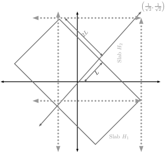
Figure 1. A geometric sketch of the bound for $Q_{2}[X_{T_{B_{L,2L,l}}(0)}\notin\partial^{+}B_{L,2L,l}(0)]$.

In virtue of the claim (15) the last expression has an exponential bound and this finishes the proof. ∎

3. Preliminary discussion

In this section we will derive some important properties that are satisfied by the non-effective polynomial and cone mixing conditions. In subsection 3.1 we will show that the non-effective polynomial condition is weaker than the conditional form of Kalikow’s condition introduced in [CZ02]. In subsection 3.2 we will show that the cone mixing condition implies ergodicity. Finally, in subsection 3.3, we will prove that the non-effective polynomial condition in a given direction implies the non-effective polynomial condition in a neighborhood of that direction with a lower degree.

3.1. Non-effective polynomial condition and its relation with other directional transience conditions

Here we will discuss the relationship between the condition non-effective polynomial condition and other transience conditions. Furthermore we will show that the conditional non-effective polynomial condition is weaker than the conditional version of Kalikow’s condition introduced by Comets-Zeitouni in [CZ01] and [CZ02].

For reasons that will become clear in the next section, the following definition, which is actually weaker than the conditional non-effective polynomial condition, will be useful. Let $l\in\mathbb{S}^{d-1}$, $M\geq 1$ and $c>0$. We say that condition $(P)_{M,c}|l$ is satisfied, and we call it the non-effective polynomial condition if there is a constant $c>0$ such that

$$\overline{\lim}_{L\to\infty}L^{M}P_{0}[X_{T_{B_{L,cL,l}}(0)}\not\in\partial^{+}B_{L,{c}L,l}(0)]=0.$$

It is straightforward to see that $(PC)_{M,c}|l$ implies $(P)_{M,c}|l$.

It should be pointed out, that for a fixed $\gamma\in(0,1)$, if both in the conditional and non-conditional non-effective polynomial conditions the polynomial decay is replaced by a stronger stretched exponential decay of the form $e^{-L^{\gamma}}$, one would obtain a condition defined on rectangles equivalent to condition $(T)_{\gamma}$ introduced by Sznitman in [Sz03], and also a conditional version of it. On the other hand, as we will see now, the conditional non-effective polynomial condition is implied by Kalikow’s condition as defined in [CZ01] for environments which are not necessarily i.i.d. Let us recall this definition. For $V$ a finite, connected subset of $\mathbb{Z}^{d}$, with $0\in V$ , we let

$$\mathfrak{F}_{V^{c}}=\sigma\{\omega(z,\cdot):z\not\in V\}.$$

The Kalikow’s random walk $\{X_{n}:n\geq 0\}$ with state space in $V\cup\partial V$, starting from $y\in V\cup\partial V$ is defined by the transition probabilities

$$\widehat{P}_{V}(x,x+e):=\left\{\begin{array}[]{ll}\frac{E_{0}[\sum_{n=0}^{T_{V^{c}}}\mathds{1}_{\{X_{n}=x\}}\omega(x,e)|\mathfrak{F}_{V^{c}}]}{E_{0}[\sum_{n=0}^{T_{V^{c}}}\mathds{1}_{\{X_{n}=x\}}|\mathfrak{F}_{V^{c}}]},&\quad{\rm for}\quad x\in V\ {\rm and}\ e\in E\\ 1&\quad{\rm for}\quad x\in\partial V\ {\rm and}\ e=0.\end{array}\right.$$

We denote by $\hat{P}_{y,V}$ the law of this random walk and by $\hat{E}_{y,V}$ the corresponding expectation. The importance of Kalikow’s random walk stems from the fact that

$$X_{T_{V^{c}}}\ \ \mbox{has the same law under }\widehat{P}_{0,V}\ \mbox{and under }P_{0}[\cdot|\mathfrak{F}_{V^{c}}]$$ (16)

(see ([K81])). Let $l\in\mathbb{S}^{d-1}$. We now define Kalikow’s condition with respect to the direction $l$ as the following requirement: there exits a positive constant $\delta$ such that

$$\inf_{V:x\in V}\ \widehat{d}_{V}(x)\cdot l\geq\delta,$$

where

$$\widehat{d}_{V}(x):=\widehat{E}_{x,V}[X_{1}-X_{0}]=\sum_{e\in E}e\widehat{P}_{V}(x,x+e)$$

denotes the drift of Kalikow’s random walk at $x$, and the infimum runs over all finite connected subset $V$ of $\mathbb{Z}^{d}$ such that $0\in V$. The following result shows that Kalikow’s condition is indeed stronger that the conditional non-effective polynomial criteria.

Proposition 3.1.

Let $l\in\mathbb{S}^{d-1}$. Assume Kalikow’s condition with respect to $l$. Then there exists an $r>0$ such that for all $y\in H_{0,l}$ one has that

$$\!\!\!\!\textcopyright∂\displaystyle\limsup_{\begin{subarray}{c}L\to\infty\end{subarray}}L^{-1}\sup\log P_{0}[X_{T_{B_{L,rL,l}}(0)}\not\in\partial^{+}B_{L,rL,l}(0),T_{B_{L,rL,l}(0)}<T_{H_{y,l}}|\mathcal{H}_{y,l}]$$

$$<0,$$

where the supremum is taken in the same sense as in (5). In particular, Kalikow’s condition with respect to direction $l$ implies $(PC)_{M,r}|l$ for all $M>0$.

Proof.

Suppose that Kalikow’s condition is satisfied with constant $\delta>0$. We will first assume that $y\cdot l\in(-L,0)$. Let $c>1$. For $y\in H_{0,l}$ and $L\geq 1$ consider the box

$$V:=R\left([y\cdot l,L]\times\left(-\frac{c}{\delta}L,\frac{c}{\delta}L\right)^{d-1}\right).$$

Therefore, using (16) we find that

$$P_{0}[X_{T_{B_{L,\frac{c}{\delta}L,l}}(0)}\not\in\partial^{+}B_{L,cL,l}(0),T_{B_{L,\frac{c}{\delta}L,l}(0)}<T_{H_{y,l}}|\mathfrak{F}_{V^{c}}]$$

$$\leq P_{0}[X_{T_{\widetilde{U}}}\cdot R(e_{j})\geq\frac{c}{\delta}L\mbox{ for some }j\in[2,d],|X_{T_{\widetilde{U}}}\cdot l|<L|\mathfrak{F}_{V^{c}}]$$

$$=\widehat{P}_{0,V}[X_{T_{\widetilde{U}}}\cdot R(e_{j})\geq\frac{c}{\delta}L\mbox{ for some }j\in[2,d],|X_{T_{\widetilde{U}}}\cdot l|<L].$$ (17)

Notice that on the set

$$\{X_{T_{V}}\cdot R(e_{j})\geq\frac{c}{\delta}L\mbox{ for some }j,X_{T_{V}}\cdot l<L\},$$

one has $\widehat{P}_{0,V}$-a.s. that

$$T_{V}\geq\left[\frac{cL}{\delta}\right].$$

Thus, by means of the auxiliary martingale $\{M_{n}^{V}:n\geq 0\}$ defined by

$$M_{n}^{V}:=X_{n}-X_{0}-\sum_{j=0}^{n-1}\widehat{d}_{V}(X_{j}),$$

which has bounded increments (indeed bounded by $2$) we can see that on $\{T_{V}>\left[\frac{cL}{\delta}]\right\}$, we have that for $L$ large enough that

$$M_{[\frac{cL}{\delta}]}^{V}\cdot l<L-\left(\frac{cL}{\delta}-1\right)\delta=(1-c)L+\delta<\frac{(1-c)L}{2}$$ (18)

$\widehat{P}_{0,V}$-a.s. Now, it will be convenient at this point to recall Azuma’s inequality (see for example [Sz01]) for martingales with increments bounded by $2$,

$$\widehat{P}_{0,V}[M_{n}^{V}\cdot w>A]\leq\exp\left\{-\frac{A^{2}}{8n}\right\}\ \mbox{ for }\ A>0,\ n\geq 0,\ |w|=1.$$

Using this inequality and (18) we obtain that

$$\widehat{P}_{0,V}[X_{T_{\widetilde{U}}}\cdot R(e_{j})>\frac{c}{\delta}L\mbox{ for some }j,X_{T_{V}}\cdot l\leq L]$$

$$\leq\widehat{P}_{0,V}[T_{V}>\frac{cL}{\delta}]$$

$$\leq\widehat{P}_{0,V}[M_{[\frac{cL}{\delta}]}^{V}\cdot(-l)>(c-1)L/2]\leq\exp\{-c_{1}L\},$$ (19)

for a suitable positive constant $c_{1}$. Finally, coming back to (17), we can then conclude that

$$\limsup_{\begin{subarray}{c}L\to\infty\end{subarray}}L^{-1}\sup\log P_{0}[X_{T_{B_{L,rL,l}}(0)}\not\in\partial^{+}B_{L,rL,l}(0),T_{B_{L,rL,l}(0)}<T_{H_{y,l}}|\mathcal{H}_{y,l}]<0,$$

where $r=\frac{c}{\delta}$. Let us now assume that $y\cdot l\leq-L$. By Lemma 1.1 in [Sz01] we know that there exists a positive constant $\psi$ depending on $\delta$ such that for all $V$ finite connected subsets of $\mathbb{Z}^{d}$ with $0\in V$

$$e^{-\psi X_{n}\cdot l}$$

is a supermartingale with respect to the canonical filtration of the walk under Kalikow’s law $\widehat{P}_{0,V}$. Thus, we have that

$$\widehat{P}_{0,V}[X_{T_{V}}\cdot l\leq-L]\leq\exp\{-\psi L\}$$

by means of the stopping time theorem applied at time $T_{V}$. By an argument similar to the one developed for the case $y\cdot l\in(-L,0)$, we can finish the estimate in the case $y\cdot l\leq L$. ∎

3.2. Cone mixing and ergodicity

The main objective in this section is to establish that any stationary probability measure $\mathbb{P}$ defined on the canonical $\sigma-$ algebra $\mathfrak{F}$, which satisfies property $(CM)_{\phi,\alpha}|l$ is ergodic with respect to space-shifts. We do not claim any originality about such an implication, but since we where not able to find an adecuate reference, we have included the proof of it here for completeness.

Let us recall that a set $E\in\mathfrak{F}$ is an invariant set if

$$\theta^{-1}_{x}E:=E$$

for all $x\in\mathbb{Z}^{d}$.

Theorem 3.2.

Assume that the probability space $(\Omega,\mathfrak{F},\mathbb{P})$ has the property $(CM)_{\phi,\alpha}|l$ and is stationary, then the probability measure $\mathbb{P}$ is ergodic, i.e. for any invariant set $E\in\mathfrak{F}$ we have:

$$\mathbb{P}[E]\in\{0,1\}.$$

Proof.

Let $E\in\mathfrak{F}$ be an invariant set. Note that for each $\epsilon>0$ there exists a cylinder measurable set $A\in\mathfrak{F}$ such that

$$\mathbb{P}[A\triangle E]<\epsilon.$$

Since $A$ is a cylinder measurable set, it can be represented as

$$A=\{\omega(x,\cdot):\ x\in F,F\subset\mathbb{Z}^{d},\ |F|<\infty,$$

$$\omega(x_{i},\cdot)\in P_{i},\mbox{ for $x_{i}\in F$},\ P_{i}\in\mathcal{B}(\mathcal{P}_{d})\},$$

where $\mathcal{B}(\mathcal{P}_{d})$ stands for the Borel $\sigma-$algebra on the compact subset $\mathcal{P}_{d}$ of $\mathbb{R}^{2d}$. Choose now $L$ such that

$$\phi(L)<\epsilon.$$

Plainly, for $L$ we can find an $x\in\mathbb{Z}^{d}$ such that $\theta_{x}A$ and $A$ are $L$ separated on cones with respect to direction $l$: there exists $y\in\mathbb{Z}^{d}$ such that

$$A\in\sigma\{\omega(z,\cdot):\ z\cdot l\leq y\cdot l-L\}$$

along with

$$\theta_{x}A\in\sigma\{\omega(z,\cdot):\ z\in C(y,l,\alpha)\}.$$

We can suppose that $\mathbb{P}[E]>0$, otherwise there is nothing to prove. So as to complete the proof we have to show that $\mathbb{P}[E]=1$. Therefore taking $\epsilon$ small enough we can suppose that $\mathbb{P}[A]>0$. Thus, using the cone mixing property, we get that

$$-\mathbb{P}[A]\phi(L)\leq\mathbb{P}[A\cap(\theta_{x}A)^{c}]-\mathbb{P}[A]\mathbb{P}[\Omega-A]\leq\mathbb{P}[A]\phi(L).$$ (20)

On the other hand, since $E$ is an invariant set, we see that

$$\mathbb{P}[\theta_{x}A\triangle E]=\mathbb{P}[\theta_{x}A\triangle\theta_{x}E]=\mathbb{P}[\theta_{x}(A\triangle E)]<\epsilon,$$ (21)

which implies

$$\mathbb{P}[A\triangle\theta_{x}A]\leq\mathbb{P}[(A\triangle E)\cup(\theta_{x}A\triangle\theta_{x}E)]<2\epsilon.$$ (22)

In turn, from inequality (22), it is clear that $\mathbb{P}[A\cap(\theta_{x}A)^{c}]<2\epsilon$. Now, using the inequality (20) one has that

$$\mathbb{P}[A]\mathbb{P}[\Omega-A]\leq 2\epsilon+\mathbb{P}[A]\phi(L).$$

As a result, we see that

$$\mathbb{P}[E]\mathbb{P}[\Omega-E]<(\mathbb{P}[A]+\epsilon)(\mathbb{P}[\Omega-A]+\epsilon)$$

$$=\mathbb{P}[A]\mathbb{P}[\Omega-A]+\epsilon+\epsilon^{2}<4\epsilon+\phi(L)\leq 5\epsilon.$$

Hence, since $\epsilon>0$ is arbitrary we conclude that $\mathbb{P}[E]\mathbb{P}[\Omega-E]=0$. Therefore if $\mathbb{P}[E]>0$, this implies $\mathbb{P}[E]=1$. ∎

3.3. Polynomial Decay implies Polynomial decay in a neighborhood

In this subsection we prove that whenever $(PC)_{M,c}|l$ holds, for prescribed positive constants $M$ and $c$, then we can choose $2(d-1)$ directions where we still have polynomial decay although of less order. More precisely, we can prove the following.

Proposition 3.3.

Suppose that $(P)_{M,c}|l$ is satisfied with $c>0$ for some $M>6(d-1)$, then there exists an $\alpha>0$ such that if we define for $i\in[2,d]$,

$$l_{+i}:=\frac{l+\alpha R(e_{i})}{|l+\alpha R(e_{i})|}$$

and

$$l_{-i}:=\frac{l-\alpha R(e_{i})}{|l-\alpha R(e_{i})|},$$

then

$$(P)_{N,2c}|l_{\pm i}$$

is satisfied with $N=\frac{M}{3}-1$.

Proof of Proposition 3.3.

We will just give the proof for direction $l_{-2}$, the other cases being analogous. Throughout the proof we pick $\alpha\in(0,1)$ and we define the angle

$$\beta:=\arctan(\alpha).$$ (23)

Consider the rotation $R^{\prime\prime}$ on $\mathbb{R}^{d}$ defined by

$$R^{\prime\prime}:=\left(\begin{array}[]{cccccc}\cos(\beta)&-\sin(\beta)&0&\ldots&\ldots&0\\ \sin(\beta)&\cos(\beta)&0&\ldots&\ldots&0\\ 0&0&1&\ldots&\ldots&0\\ \vdots&\vdots&\vdots&\vdots&\vdots&\vdots\\ \vdots&\vdots&\vdots&\vdots&\vdots&\vdots\\ 0&0&\ldots&\ldots&1&0\\ 0&0&\ldots&\ldots&0&1\\ \end{array}\right).$$

where this representation matrix is taken in the vector space base $\{R(e_{1}),R(e_{2}),\ldots,R(e_{d})\}$. It will be useful to define a new rotation

$$R^{\prime}:=R^{\prime\prime}R$$

together with the rotated box $\widetilde{B}_{L}(0)$ given by

$$\widetilde{B}_{L}(0):=R^{\prime}\left(\left[-L\lambda_{1}(\alpha),L\lambda_{2}(\alpha)\right]\times\left[-Lc\lambda_{3}(\alpha),Lc\lambda_{3}(\alpha)\right]^{d-1}\right)\cap\mathbb{Z}^{d},$$

where

$$\lambda_{1}(\alpha):=\frac{1+\frac{1}{\alpha}}{\sqrt{\cot^{2}(\beta)+1}}$$

$$\lambda_{2}(\alpha):=\frac{\frac{1}{\alpha}-1}{\sqrt{\cot^{2}(\beta)+1}}$$

$$\lambda_{3}(\alpha):=\frac{\sqrt{(1-\cot(\beta))^{2}+(1-\tan(\beta))^{2}}}{|\tan(\beta)+\cot(\beta)|}$$

Notice that with these definitions, $P_{0}$- almost surely:

$$X_{T_{\widetilde{B}_{L}(0)}}\not\in\partial^{+}\widetilde{B}_{L}(0)\Rightarrow X_{T_{B_{L,L,l}(0)}}\not\in\partial^{+}B_{L,L,l}(0).$$ (24)

Figure 2 shows the boxes involved in (24).

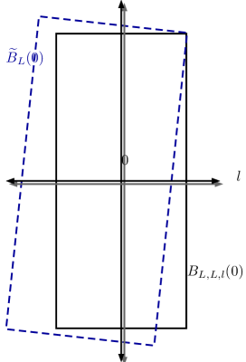
Figure 2. The choice of boxes.

As a result we have that

$$P_{0}[X_{T_{\widetilde{B}_{L}(0)}}\not\in\partial^{+}\widetilde{B}_{L}(0)]\leq L^{-M}.$$

Furthermore, a straightforward computation makes us see that the scale factor $\lambda_{3}(\alpha)$ is less than $\frac{4}{3}$ whenever $\alpha\leq\frac{1}{9}$. Therefore if we let the positive $\alpha\leq\frac{1}{9}$ one has that

$$\lambda_{3}(\alpha)\leq\frac{4}{3}.$$ (25)

For technical reasons, we need to introduce an auxiliary box. Specifically, we first set

$$h:=\frac{\frac{1}{\alpha}-1}{\sqrt{1+(\frac{1}{\alpha})^{2}}}=\frac{1-\alpha}{\sqrt{1+\alpha^{2}}}$$

and observe that $\frac{4}{5}<h<1$. We then can introduce the new box $\overline{B}_{l_{-2},L}(0)$ defined by

$$\overline{B}_{l_{-2},L}(0):=R^{\prime}\left(\left[-L(h+2),Lh\right]\times\left[-cL\lambda_{3}(\alpha),Lc\lambda_{3}(\alpha)\right]^{d-1}\right)\cap\mathbb{Z}^{d}.$$

From this definition, we obtain

$$P_{0}[X_{T_{\overline{B}_{l_{-2},L}(0)}}\not\in\partial^{+}\overline{B}_{l_{-2},L}(0)]\leq L^{-M}.$$

In order to complete the proof, we claim that for large enough $U$ the probability

$$P_{0}[X_{T_{\overline{B}_{l_{-2},U}(0)}}\not\in\partial^{+}\overline{B}_{l_{-2},U}(0)],$$

decays polynomially as a function of $U$, where the box $\overline{B}_{l_{-2},U}(0)$ is defined by

$$\overline{B}_{l_{-2},U}(0):=R^{\prime}([-U,U]\times[-2cU,2cU]^{d-1}).$$

The general strategy to follow will be to stack smaller boxes up inside of $\overline{B}_{l_{-2},U}(0)$ and then using the Markov property along with good environment sets we ensure that the walk exits from box $\overline{B}_{l_{-2},U}(0)$ by $\partial^{+}\overline{B}_{l_{-2},U}(0)$ with probability bigger than $1-P(U)$, where $P$ is a polynomial function. Specifically, we let

$$L:=\frac{U}{h+2}.$$ (26)

Introduce now a sequence of stopping times as follows

$$T_{1}=T_{\overline{B}_{l_{-2},L}(0)},$$

and for $i>1$

$$T_{i}=T_{i-1}+T_{1}\circ\theta_{T_{i-1}}.$$

For simplicity we write $\widehat{T_{1}}$ instead of $T_{\overline{B}_{l_{-2},U}(0)}.$ In view of (25) and (26) it is clear that to ensure that the random walk exits at time $\widehat{T}_{1}$ through $\partial^{+}\bar{B}_{l_{-2},U}(0)$, it is enough that it exits through the corresponding positive boundaries through four succesive times, so that

$$P_{0}[X_{\widehat{T_{1}}}\in\partial^{+}\overline{B}_{l_{-2},U}(0)]\geq P_{0}\left[X_{T_{1}}\in\partial^{+}\overline{B}_{l_{-2},L}(0),\right.$$

$$\left.\left(X_{T_{1}}\in\partial^{+}\overline{B}_{l_{-2},L}(X_{T_{1}})\right)\circ\theta_{T_{1}},\left(X_{T_{1}}\in\partial^{+}\overline{B}_{l_{-2},L}(X_{T_{2}})\right)\circ\theta_{T_{2}},\right.$$

$$\left.\left(X_{T_{1}}\in\partial^{+}\overline{B}_{l_{-2},L}(X_{T_{3}})\right)\circ\theta_{T_{3}}\right].$$ (27)

In order to use (27), let $i$ be a positive integer number and consider the lattice sets sequence $(F_{i})_{i\geq 1}$ defined by

$$F_{1}=\partial^{+}\overline{B}_{l_{-2},L}(0),$$

and for $i>1$, we define by induction

$$F_{i}=\bigcup_{y\in F_{1}}\partial^{+}\overline{B}_{l_{-2},L}(y).$$

We now define for $i\geq 1$, the environment events $G_{i}$ by

$$G_{i}=\left\{\omega\in\Omega:P_{y,\omega}[\left(X_{T_{1}}\in\partial^{+}\overline{B}_{l_{-2},L}(X_{T_{i}})\right)\circ\theta_{T_{i}}]\right.$$

$$\left.\geq 1-L^{-\frac{M}{2}},\mbox{ for each }y\in F_{i}\right\}.$$

Note that

$$P_{0}[X_{\widehat{T_{1}}}\in\partial^{+}\overline{B}_{l_{-2},U}(0)]$$

$$\geq P_{0}\left[X_{T_{1}}\in\partial^{+}\overline{B}_{l_{-2},L}(0),\left(X_{T_{1}}\in\partial^{+}\overline{B}_{l_{-2},L}(X_{T_{1}})\right)\circ\theta_{T_{1}},\right.$$

$$\left.\left(X_{T_{1}}\in\partial^{+}\overline{B}_{l_{-2},L}(X_{T_{2}})\right)\circ\theta_{T_{2}},\left(X_{T_{1}}\in\partial^{+}\overline{B}_{l_{-2},L}(X_{T_{3}})\right)\circ\theta_{T_{3}}\mathds{1}_{G_{3}}\right].$$

By the Markov property applied at time $T_{3}$ and the very meaning of $G_{3}$, we get that the last expression is equal to

$$\sum_{y\in F_{3}}\mathbb{E}\left[P_{0,\omega}\left[X_{T_{1}}\in\partial^{+}\overline{B}_{l_{-2},L}(0),\left(X_{T_{1}}\in\partial^{+}\overline{B}_{l_{-2},L}(X_{T_{1}})\right)\circ\theta_{T_{1}},\right.\right.$$

$$\left.\left.\left(X_{T_{1}}\in\partial^{+}\overline{B}_{l_{-2},L}(X_{T_{2}})\right)\circ\theta_{T_{2}}\right]P_{y,\omega}[X_{T_{\overline{B}_{l_{-2},L}(y)}}\in\partial^{+}\overline{B}_{l_{-2},L}(y)]\mathds{1}_{G_{3}}\right]\geq$$

$$(1-L^{-\frac{M}{2}})\left(P_{0}\left[X_{T_{1}}\in\partial^{+}\overline{B}_{l_{-2},L}(0),\left(X_{T_{1}}\in\partial^{+}\overline{B}_{l_{-2},L}(X_{T_{1}})\right)\circ\theta_{T_{1}},\right.\right.$$

$$\left.\left.\left(X_{T_{1}}\in\partial^{+}\overline{B}_{l_{-2},L}(X_{T_{2}})\right)\circ\theta_{T_{2}}\right]-\mathbb{P}[(G_{3})^{c}]\right).$$ (28)

Repeating the above argument, one has the following upper bound for the right-most expression of (28),

$$(1-L^{-\frac{M}{2}})^{4}-(1-L^{-\frac{M}{2}})^{3}\mathbb{P}[(G_{1})^{c}]-(1-L^{-\frac{M}{2}})^{2}\mathbb{P}[(G_{2})^{c}]-(1-L^{-\frac{M}{2}})\mathbb{P}[(G_{3})^{c}].$$ (29)

At this point, we would like to obtain for $i\in|[1,3]|$, an upper bound of the probabilities

$$\mathbb{P}[(G_{i})^{c}].$$

To this end, we first observe that Chebyshev’s inequality and our hypothesis imply

$$\mathbb{P}[(G_{1})^{c}]\leq\sum_{y\in F_{1}}\mathbb{E}[\mathds{1}_{\{P_{y,\omega}[X_{T_{\overline{B}_{l_{-2},L}(y)}}\in\partial^{+}\overline{B}_{l_{-2},L}(y)]>L^{-\frac{M}{2}}\}}]\leq\mid F_{1}\mid L^{-\frac{M}{2}}.$$

Clearly, we have the estimate $\mid F_{1}\mid\leq\left(\frac{8}{3}L\right)^{d-1}$ (recall (25)). As a result, we see that

$$\mathbb{P}[(G_{1})^{c}]\leq\left(\frac{8}{3}L\right)^{d-1}L^{-\frac{M}{2}}.$$ (30)

By a similar procedure we can conclude that

$$\mathbb{P}[(G_{2})^{c}]\leq\left(\frac{16}{3}L\right)^{d-1}L^{-\frac{M}{2}}\quad{\rm and}\quad\mathbb{P}[(G_{3})^{c}]\leq\left(\frac{24}{3}L\right)^{d-1}L^{-\frac{M}{2}}.$$ (31)

Combining the estimates in (27) and (31) and the assumption $M\geq 6(d-1)$ we see that

$$P_{0}[X_{\widehat{T_{1}}}\not\in\partial^{+}\overline{B}_{l_{-2},U}(0)]\leq 3\frac{6(8)^{d-1}}{2^{-\frac{M}{3}}}U^{-\frac{M}{3}}.$$

This ends the proof by choosing the required $\alpha$ as any number in the open interval $(0,\frac{1}{9})$. ∎

4. Backtracking of the random walk out of a cone

Here we will provide a uniform control on the probability that a random walk starting form the vertex of a cone stays inside the cone forever. It will be useful to this end to define

$$D^{\prime}:=\inf\{n\in\mathbb{N}:X_{n}\not\in\mathcal{C}(\alpha,l,X_{0})\},$$ (32)

where as before $l\in\mathbb{S}^{d-1}$.

Proposition 4.1.

Let $l\in\mathbb{S}^{d-1}$. Suppose that $(P)_{M,c}|l$ holds, for some $M>6d-3$. Then there exists a positive constant $c_{2}(d)>0$ such that $P_{0}[D^{\prime}=\infty]>c_{2}(d)$.

In what follows we prove this proposition. With the purpose of making easier the reading, we introduce here some notations. Let $l^{\prime}\in\mathbb{S}^{d-1}$ and choose a rotation $R^{\prime}$ on $\mathbb{R}^{d}$ with the property

$$R^{\prime}(e_{1})=l^{\prime}$$

For each $x\in\mathbb{Z}^{d}$, real numbers $m>0$, $c>0$ and integer $i\geq 0$ we define the box

$$B_{i}(x):=$$

$$x+R^{\prime}\left(\left(-2^{m+i},2^{m+i}\right)\times\left(-2c2^{m+i},2c2^{m+i}\right)^{d-1}\right)\cap\mathbb{Z}^{d}$$

along with its ”positive boundary”

$$\partial^{+}B_{i}(x):=\partial B_{i}(x)\cap\{x+R^{\prime}\left((2^{m+i},\infty)\times\mathbb{R}^{d-1}\right)\}.$$

We also need slabs perpendicular to direction $l^{\prime}$. Set

$$V_{0}(x):=x+R^{\prime}\left([-2^{m},2^{m}]\times\mathbb{R}^{d-1}\right)\cap\mathbb{Z}^{d}$$

and for $i\geq 1$,

$$V_{i}(x):=x+R^{\prime}\left(\left[-2^{m},\sum_{j=0}^{i}2^{m+j}\right]\times\mathbb{R}^{d-1}\right)\cap\mathbb{Z}^{d}.$$

The positive part of the boundary for this set is defined as

$$\partial^{+}V_{i}(x):=\partial V_{i}(x)\cap\left\{x+R^{\prime}\left(\left(\sum_{j=0}^{i}2^{m+j},\infty\right)\times\mathbb{R}^{d-1}\right)\right\}.$$

Furthermore, we will define recursively a sequence of stopping times as follows. First, let

$$T_{0}:=T_{B_{0}(X_{0})}.$$

and for $i\geq 1$

$$T_{i}:=T_{B_{i}(X_{T_{i-1}})}\circ\theta_{T_{i-1}}+T_{i-1}.$$

We now need to define the first time of entrance of the random walk to the hyperplane $R^{\prime}\left((-\infty,0)\times\mathbb{R}^{d-1}\right)$,

$$D_{l^{\prime}}:=\inf\{n\geq 0:X_{n}\cdot l^{\prime}<0\}.$$

With these notations we can prove:

Lemma 4.2.

Assume $(P)_{N,2c}|l^{\prime}$ where $c>0$ , for some $N>2(d-1)$. Then, for all $m\in\mathbb{N}$ and $x\in\{z\in\mathbb{Z}^{d}:z\cdot l^{\prime}\geq 2^{m}\}$, we have that

$$P_{x}[D_{l^{\prime}}=\infty]\geq y(m)$$

where $y(m)$ does not depend on $l^{\prime}$ and satisfies $\lim_{m\rightarrow\infty}y(m)=1$.

Proof.

From the fact that $(P)_{N,2}|l^{\prime}$ holds, we can (and we do) assume that there exists a $m>0$ large enough, such that for any positive integer $i$ one has that

$$P_{0}[X_{T_{B_{i}(0)}}\in\partial^{+}B_{i}(0)]\geq 1-2^{-N(m+i)}$$ (33)

holds. By stationarity, we have for $x\in\mathbb{Z}^{d}$:

$$P_{x}[X_{T_{B_{i}(x)}}\in\partial^{+}B_{i}(x)]\geq 1-2^{-N(m+i)}.$$ (34)

Throughout this proof, let us choose $x\in\{z\in\mathbb{Z}^{d}:z\cdot l^{\prime}\geq 2^{m}\}$. For reasons that will be clear through the proof, we need to estimate for $i\geq 1$ the following probability

$$I_{i}:=P_{x}[X_{T_{V_{i}(x)}}\in\partial^{+}V_{i}(x)],$$ (35)

and with this aim, in view of (34), we have

$$I_{0}\geq P_{x}[X_{T_{B_{0}(x)}}\in\partial^{+}B_{0}(x)]\geq 1-2^{-Nm}\geq 1-2^{-N\frac{m}{2}}.$$

Now, as a preliminary computation for the recursion, we begin to estimate $I_{1}$. Note that

$$I_{1}\geq P_{x}[X_{T_{0}}\in\partial^{+}B_{0}(X_{0}),(X_{T_{B_{1}(X_{0})}}\in\partial^{+}B_{1}(X_{0}))\circ\theta_{T_{0}}].$$ (36)

Using the strong Markov property at time $T_{0}$ we then see that

$$I_{1}\geq\sum_{y\in\partial^{+}B_{0}(x)}\mathbb{E}\left[P_{x,\omega}[X_{T_{0}}\in\partial^{+}B_{0}(X_{0}),X_{T_{0}}=y]\right.$$

$$\times\left.P_{y,\omega}[X_{T_{B_{1}(y)}}\in\partial^{+}B_{1}(y)]\right]$$

$$\geq\sum_{y\in\partial^{+}B_{0}(x)}\mathbb{E}\left[P_{x,\omega}[X_{T_{0}}\in\partial^{+}B_{0}(X_{0}),X_{T_{0}}=y]\right.$$

$$\times\left.P_{y,\omega}[X_{T_{B_{1}(y)}}\in\partial^{+}B_{1}(y)]\mathds{1}_{G_{0}}\right],$$ (37)

where

$$G_{0}:=$$

$$\{w\in\Omega:P_{y,\omega}[X_{T_{B_{1}(y)}}\in\partial^{+}B_{1}(y)]>1-2^{-N\frac{m}{2}},\ \mbox{for all}\ y\in\partial^{+}B_{0}(x)\}.$$

Thus, it is clear that

$$I_{1}\geq\left(1-2^{-N\frac{m}{2}}\right)\left(P_{x}[X_{T_{0}}\in\partial^{+}B_{0}(X_{0})]-\mathbb{P}[(G_{0})^{c}]\right).$$ (38)

Notice that by (34) and Chebyshev’s inequality

$$\mathbb{P}[(G_{0})^{c}]\leq\sum_{y\in\partial^{+}B_{0}(x)}\mathbb{P}[P_{y,\omega}[X_{T_{B_{1}(y)}}\not\in\partial^{+}B_{1}(y)]\geq 2^{-N\frac{m}{2}}]$$

$$\leq\sum_{y\in\partial^{+}B_{0}(x)}P_{y}[X_{T_{B_{1}(y)}}\not\in\partial^{+}B_{1}(y)]2^{N\frac{m}{2}}$$

$$=|\partial^{+}B_{0}(x)|2^{N\frac{m}{2}}]P_{0}[X_{T_{B_{1}(0)}}\not\in\partial^{+}B_{1}(0)]$$

$$\leq(2c2^{m+1})^{d-1}2^{N\left(\frac{m}{2}-(m+1)\right)}\leq(2c2^{m+1})^{d-1}2^{-N\frac{m}{2}}.$$ (39)

Plugging (39) into (38) we see that

$$I_{1}\geq(1-2^{-N\frac{m}{2}})(1-2^{-N\frac{m}{2}}-(2c2^{m+1})^{d-1}2^{-N\frac{m}{2}}).$$ (40)

Hereafter we can do the general recursive procedure. For this end, we define for $i\geq 1$

$$\begin{split}J_{i}:=P_{0}[X_{T_{0}}\in\partial^{+}B_{0}(X_{0}),(X_{T_{B_{1}(X_{0})}}\in\partial^{+}B_{1}(X_{0}))\circ\theta_{T_{0}},\ldots\\ \ldots,(X_{T_{B_{i}(X_{0})}}\in\partial^{+}B_{i}(X_{0}))\circ\theta_{T_{i-1}}].\end{split}$$ (41)

It is straightforward that $I_{i}\geq J_{i}$. Furthermore, through induction on $i\geq 1$, we will establish the following claim

$$J_{i}\geq(1-2^{-N\frac{(m+i-1)}{2}})\left[J_{i-1}-2^{-N\frac{(m+i-1)}{2}}\left(\sum_{j=0}^{i-1}2c2^{(m+j)+1}\right)^{d-1}\right].$$ (42)

To prove this, we first define the extended boundary of the pile of boxes at a given step as

$$F_{0}:=\partial B_{0}(x)\cap\{x+R^{\prime}((2^{m},\infty)\times\mathbb{R}^{d-1}))\},$$

and for $i\geq 2$

$$F_{i-1}:=\partial\left\{\cup_{y\in F_{i-2}}B_{i-1}(y)\right\}\cap\{x+R^{\prime}((2^{m+i-1},\infty)\times\mathbb{R}^{d-1}))\}.$$

Using these notations, we can apply the strong Markov property to (41) at time $T_{i-1}$, to get that

$$J_{i}=\sum_{y\in F_{i-1}}\mathbb{E}\left[P_{x,\omega}[X_{T_{0}}\in\partial^{+}B_{0}(X_{0}),\ldots\right.$$

$$\left.\ldots,(X_{T_{B_{i-1}(X_{0})}}\in\partial^{+}B_{i-1}(X_{0}))\circ\theta_{T_{i-2}},X_{T_{i-1}}=y]P_{y,\omega}[X_{T_{B_{i}(X_{0})}}\in\partial^{+}B_{i}(X_{0})]\right].$$

Following the same strategy used to deduce (40), it will be convenient to introduce for each $i\geq 2$ the event

$$G_{i-1}:=$$

$$\{\omega\in\Omega:P_{y,\omega}[X_{T_{B_{i}(y)}}\in\partial^{+}B_{i}(y)]>1-2^{-N\frac{(m+i-1)}{2}},\ \mbox{for all}\ y\in F_{i-1}\}.$$

Inserting the indicator function of the event $G_{i-1}$ into (41) we get that

$$J_{i}\geq$$

$$\sum_{y\in F_{i-1}}\mathbb{E}\left[P_{x,\omega}[X_{T_{0}}\in\partial^{+}B_{0}(X_{0}),\ldots,(X_{T_{B_{i-1}(X_{0})}}\in\partial^{+}B_{i-1}(X_{0}))\circ\theta_{T_{i-2}},X_{T_{i-1}}=y]\right.$$

$$\left.\times P_{y,\omega}[X_{T_{B_{i}(X_{0})}}\in\partial^{+}B_{i}(X_{0})]\mathds{1}_{G_{i-1}}\right].$$

By the same kind of estimation as in (38), we have

$$J_{i}\geq(1-2^{-N\frac{(m+i-1)}{2}})\left(J_{i-1}-\mathbb{P}[(G_{i-1})^{c}]\right).$$ (43)

We need to get an estimate for $\mathbb{P}[(G_{i-1})^{c}]$. We do it repeating the argument given in (39). Let us first remark that

$$|F_{i-1}|\leq\left(\sum_{j=0}^{i-1}2c2^{(m+j)+1}\right)^{d-1},$$ (44)

holds. Indeed, the case in which $l^{\prime}=e_{1}$ gives the maximum number for $|F_{i-1}|$. Keeping (44) in mind we get that

$$P_{x}[(G_{i-1})^{c}]\leq\sum_{y\in F_{i-1}}\mathbb{P}\left[P_{y,\omega}\left[X_{T_{B_{i}(y)}}\not\in\partial^{+}B_{i}(y)\right]\geq 2^{-N\frac{(m+i-1)}{2}}\right]$$

$$\leq\sum_{y\in F_{i-1}}P_{y}[X_{T_{B_{i}(y)}}\not\in\partial^{+}B_{i}(y)]2^{N\frac{(m+i-1)}{2}}$$

$$\leq\left(\sum_{j=0}^{i-1}2c2^{(m+j)+1}\right)^{d-1}2^{-N\frac{(m+i-1)}{2}}.$$ (45)

Therefore, combining (45) and (43) we prove claim (42). Iterating (42) backward, from a given integer $i$, we have got

$$J_{i}\geq J_{1}\left[\prod_{h=1}^{i-1}(1-2^{-N\frac{(m+h)}{2}})\right]-\sum_{j=1}^{i-1}a_{j}2^{-N\frac{m+j}{2}}\prod_{k=j}^{i-1}(1-2^{-N\frac{(m+k)}{2}}),$$ (46)

where we have used for short

$$a_{j}:=\left(\sum_{i=0}^{j}c2^{(m+i)+1}\right)^{d-1}\leq(2c)^{d-1}2^{(m+j+2)(d-1)}.$$

The same argument used to derive (40) can be repeated to conclude that

$$J_{1}\geq(1-2^{-N\frac{m}{2}})(1-2^{-N\frac{m}{2}}-(2c2^{m+1})^{d-1}2^{-N\frac{m}{2}}).$$ (47)

Replacing the right hand side of (47) into (46), and together to the fact $I_{i}\geq J_{i}$, we see that

$$I_{i}\geq\left[\prod_{h=0}^{i-1}(1-2^{-N\frac{m+h}{2}})\right](1-2^{-N\frac{m}{2}})-\sum_{j=0}^{i-1}a_{j}2^{-N\frac{(m+j)}{2}}\prod_{k=j}^{i-1}(1-2^{-N\frac{(m+k)}{2}}).$$ (48)

Now we can finish the proof. First, observe that

$$P_{x}[D_{l^{\prime}}=\infty]\geq I_{\infty},$$

where as a matter of definition

$$I_{\infty}:=\lim_{i\rightarrow\infty}\,I_{i}$$

(this limit exists, because it is the limit of a decreasing sequence of real numbers bounded from below). By the condition $N>2(d-1)$, we get that for each $m\geq 1$ one has that for all $j\geq 1$,

$$a_{j}\ 2^{-\frac{M(m+j)}{2}}\leq(8c)^{d-1}2^{-\vartheta\frac{(m+j)}{2}},$$

where $\vartheta$ stands for the positive number so that $N=2(d-1)+\vartheta$. Thus all the products and series in (48) converge and we have that for all $m\geq 1$ and $x\in\{z\in\mathbb{Z}^{d}:z\cdot l^{\prime}\geq 2^{m}\}$

$$P_{x}[D_{l^{\prime}}=\infty]\geq y(m),$$

where

$$y(m):=\left[\prod_{h=0}^{\infty}(1-2^{-N\frac{(m+h)}{2}})\right](1-2^{-N\frac{m}{2}})$$

$$-\sum_{j=0}^{\infty}a_{j}2^{-N\frac{(m+j)}{2}}\prod_{k=j}^{\infty}(1-2^{-N\frac{(m+k)}{2}}).$$

Clearly for each $m\geq 1$, $y(m)$ does not depend on the direction $l^{\prime}$ and $\lim_{m\to\infty}y(m)=1$, which completes the proof. ∎

With the previous Lemma, we now have enough tools to prove Proposition 4.1. Before this, we need a definition of geometrical nature.

We will say that a sequence $(x_{0},\ldots,x_{n})$ of lattice points is a path if for every $1\leq i\leq n-1$, one has that $x_{i}$ and $x_{i-1}$ are nearest neighbors. Furthermore, we say that this path is admissible if for every $1\leq i\leq n-1$ one has that

$$(x_{i}-x_{i-1})\cdot l\neq 0.$$

Proof of Proposition 4.1..

Assume $(P)_{M,c}|l$, where $M>6(d-1)+3$ which is the condition of the statement of the Proposition 4.1. We appeal to Proposition (3.3) and assumption $(P)_{M,c}|l$ to choose an $\alpha>0$ such that for all $i\in[2,d]$

$$(P)_{N,2c}|l_{\pm i}$$

is satisfied with

$$N:=\frac{M}{3}-1>2(d-1).$$ (49)

From now on, let $m$ be any natural number satisfying

$$y(m)>1-\frac{1}{2(d-1)},$$ (50)

where $y(m)$ is the function given in Lemma 4.2. Note that there exists a constant $c_{3}(d)$ such that for all $x\in\mathbb{Z}^{d}$ contained in $C(\alpha,l,R(2^{m}e_{1}))$ and such that $|R(2^{m}e_{1})-x|_{1}\leq 1$ one has that there exists an admissible path with at most $c_{3}2^{m}$ lattice points joining $0$ and $x$. We denote this path by

$$(0,y_{1},\ldots,y_{n}=x)$$

noting that $n\leq c_{3}2^{m}$.

The general idea to finish the proof is to push forward the walk up to site $x$ with the help of uniform ellipticity in direction $l$ and then we make use of Lemma (4.2) to ensure that the walk remains inside the cone.

Therefore, by (49) and Lemma (4.2) we can conclude that for all $2\leq i\leq d$ one has that

$$P_{x}[D_{l_{i+}}=\infty]\geq y(m),$$ (51)

along with

$$P_{x}[D_{l_{i-}}=\infty]\geq y(m).$$ (52)

Define the event that the random walk starting from $0$ following that path $(0,y_{1},\ldots,y_{n})$ as

$$A_{n}:=\{(X_{0},\ldots,X_{n})=(0,y_{1},\ldots,y_{n})\}.$$

Now notice that

$$P_{0}[D^{\prime}=\infty]\geq$$

$$\begin{split}P_{0}\left[A_{n},(D_{l_{i-}}=\infty)\circ\theta_{n},(\ D_{l_{i+}}=\infty)\circ\theta_{n}\ {\rm for}\ 2\leq i\leq d\right].\end{split}$$ (53)

On the other hand, by definition of the annealed law, together with the strong Markov property we have that

$$P_{0}[A_{n},(D_{l_{i-}}=\infty)\circ\theta_{n},(\ D_{l_{i+}}=\infty)\circ\theta_{n}\ {\rm for}\ 2\leq i\leq d]=$$

$$\mathbb{E}\left[P_{0,\omega}[A_{n}],P_{x,\omega}[D_{l_{i-}}=\infty,D_{l_{i+}}=\infty\ {\rm for}\ 2\leq i\leq d]\right].$$ (54)

Using the uniform ellipticity assumption $(UE)|l$, along with (51) and (52), we can see that (54) is bounded from below by

$$(2\kappa)^{c_{3}2^{m}}\left(1-2(d-1)(1-y(m))\right).$$ (55)

By virtue of our choice of $m$ in (50), we see that there exists a constant $c_{2}$ just depending on the dimension (we recall that $m$ is fixed at this point of the proof), such that

$$c_{4}:=(2\kappa)^{c_{3}2^{m}}\left(1-2(d-1)(1-y(m))\right)>0$$ (56)

Finally, in view of the inequalities (53) and (54) it follows that

$$P_{0}[D^{\prime}=\infty]\geq c_{4}.$$

∎

5. Polynomial control of regeneration positions

In this section, we define an approximate regeneration times as done in [CZ01], which will depend on a distance parameter $L>0$. We will then show that these times, assuming $(PC)_{M,c}|l$ for $M$ large enough, and cone-mixing, when scaled by $\kappa^{L}$, define approximate regeneration positions with a finite second moment.

5.1. Preliminaries

We recall the definition of approximate renewal time given in [CZ01]. Let $W:=\mathcal{E}\cup\{0\}$ [c.f. (2)] and endow the space $W^{\mathbb{N}}$ with the canonical $\sigma-$algebra $\mathcal{W}$ generated by the cylinder sets. For fixed $\omega\in\Omega$ and $\varepsilon=(\varepsilon_{0},\varepsilon_{1},\ldots)\in W^{\mathbb{N}}$, we denote by $P_{\omega,\varepsilon}$ the law of the Markov chain $\{X_{n}\}$ on $(\mathbb{Z}^{d})^{\mathbb{N}}$, so that $X_{0}=0$ and with transition probabilities defined for $z\in\mathbb{Z}^{d}$, $e,|e|=1$ as

$$P_{\omega,\varepsilon}[X_{n+1}=z+e|X_{n}=z]=\mathds{1}_{\{\varepsilon_{n}=e\}}+\frac{\mathds{1}_{\{\varepsilon_{n}=0\}}}{1-\kappa|\mathcal{E}|}[\omega(z,e)-\kappa\mathds{1}_{\{e\in\mathcal{E}\}}].$$

Call $E_{\omega,\epsilon}$ the corresponding expectation. Define also the product measure $Q$, which to each sequence of the form $\varepsilon\in W^{\mathbb{N}}$ assigns the probability $Q(\varepsilon_{1}=e):=\kappa$, if $e\in\mathcal{E}$, while $Q(\varepsilon_{1}=0)=1-\kappa|\mathcal{E}|$, and denote by $E_{Q}$ the corresponding expectation.

Now let $\mathfrak{G}$ be the $\sigma$-algebra on $(\mathbb{Z}^{d})^{\mathbb{N}}$ generated by cylinder sets, while $\mathfrak{F}$ be the $\sigma$-algebra on $\Omega$ generated by cylinder sets. Then, we can define for fixed $\omega$ the measure

$$\overline{P}_{0,\omega}:=Q\otimes P_{\omega,\varepsilon}$$

on the space $(W^{\mathbb{N}}\times(\mathbb{Z}^{d})^{\mathbb{N}},\mathcal{W}\times\mathfrak{G})$, and also

$$\overline{P}_{0}:=\mathbb{P}\otimes Q\otimes P_{\omega,\varepsilon}$$

on $(\Omega\times W^{\mathbb{N}}\times(\mathbb{Z}^{d})^{\mathbb{N}},\mathfrak{F}\times\mathcal{W}\times\mathfrak{G})$, denoting by $\bar{E}_{0,\omega}$ and $\bar{E}_{0}$ the corresponding expectations. A straightforward computation makes us conclude that the law of $\{X_{n}\}$ under $\bar{P}_{0,\omega}$ coincides with its law under $P_{0,\omega}$ and that its law under $\overline{P}_{0}$ coincides with its law under $P_{0}$.

Let $q$ be a positive real number such that for all $1\leq i\leq d$,

$$u_{i}:=l_{i}q$$

is an integer. Define now the vector $u:=(u_{1},\ldots,u_{d})$. From now on, we fix a particular sequence $\overline{\varepsilon}$ in $\mathcal{E}$ of length $p:=|u|_{1}$ whose components sum up to $u$:

$$\overline{\varepsilon}:=(\overline{\varepsilon}_{1},\ldots,\overline{\varepsilon}_{p}),$$

together with

$$\overline{\varepsilon}_{1}=\overline{\varepsilon}_{2}=\ldots=\overline{\varepsilon}_{|u_{1}|}:=\ \mbox{sgn}(u_{1})e_{1},$$

$$\overline{\varepsilon}_{|u_{1}|+1}=\overline{\varepsilon}_{|u_{1}|+2}=\ldots=\overline{\varepsilon}_{|u_{1}|+|u_{2}|}:=\ \mbox{sgn}(u_{2})e_{2}$$

$$\vdots$$

$$\overline{\varepsilon}_{p-|u_{d}|+1}=\ldots=\overline{\varepsilon}_{p}:=\ \mbox{sgn}(u_{d})e_{d}.$$

Without loss of generality we can assume that $l_{1}\not=0$. And by taking $\alpha$ small enough that

$$\overline{\varepsilon}_{1},\overline{\varepsilon}_{1}+\overline{\varepsilon}_{2},\ldots\overline{\varepsilon}_{p}$$

are inside of $\mathcal{C}(0,l,\alpha)$. For $L\in p\mathbb{N}$ consider the sequence $\bar{\varepsilon}^{(L)}$ of length $L$, defined as the concatenation $L/p$ times with itself of the sequence $\bar{\varepsilon}$, so that

$$\overline{\varepsilon}^{(L)}=(\bar{\varepsilon}_{1},\ldots,\bar{\varepsilon}_{p},\ldots,\bar{\varepsilon}_{1},\ldots,\bar{\varepsilon}_{p}).$$

Consider the filtration $\mathcal{G}:=\{\mathcal{G}_{n}:n\geq 0\}$ where

$$\mathcal{G}_{n}:=\sigma((\varepsilon_{i},X_{i}),i\leq n).$$

Define $S_{0}:=0$,

$$S_{1}:=\inf\{n\geq L:\ X_{n-L}\cdot l>\max\{X_{m}\cdot l:m<n-L\},$$

$$(\varepsilon_{n-L},\ldots,\varepsilon_{n-1})=\overline{\varepsilon}^{(L)}\}$$

together with

$$R_{1}:=D^{\prime}\circ\theta_{S_{1}}+S_{1}.$$

We can now recursively define for $k\geq 1$,

$$S_{k+1}:=\inf\{n\geq R_{k}:\ X_{n-L}\cdot l>\max\{X_{m}\cdot l:m<n-L\},$$

$$(\varepsilon_{n-L},\ldots,\varepsilon_{n-1}=\overline{\varepsilon}^{(L)}))\}$$

and

$$R_{k+1}:=D^{\prime}\circ\theta_{{S}_{k+1}}+S_{k+1}.$$

Clearly,

$$0=S_{0}\leq S_{1}\leq R_{1}\leq\cdots\infty,$$

the inequalities are strict if the left member of the corresponding inequality is finite, and the sequences $\{S_{k}:k\geq 0\}$ and $\{R_{k}:k\geq 0\}$ are $\mathcal{G}$-stopping times. On the other hand, we can check that $\bar{P}_{0}-$a.s. one has that $S_{1}<\infty$ along with the fact $\bar{P}_{0}-$a.s. on the set

$$\{\lim X_{n}\cdot l=\infty\}\cap\{R_{k}<\infty\}\ \mbox{one has too that}$$ (57)

$$S_{k+1}<\infty.$$

Put

$$K:=\inf\{k\geq 1:{S}_{k}<\infty,{R}_{k}=\infty\}$$

and define the approximate regeneration time

$$\tau^{(L)}:={S}_{K}.$$ (58)

We see that the random variable $\tau^{(L)}$ is the first time $n$ in which the walk has reached a record at time $n-L$ in direction $l$, and then the walk goes on $L$ steps in the direction $l$ by means of the action of $\overline{\varepsilon}^{(L)}$ and finally after this time $n$, never exits the cone $C(X_{n},l,\alpha)$.

The following lemma is required to show that the approximate renewal times are $\bar{P}_{0}$-a.s. finite. Its can be proved using a slight variation of the argument given in page 517 of Sznitman [Sz03].

Lemma 5.1.

Consider a random walk in a random environment. Let $l\in\mathbb{S^{*}}^{d-1}$, $M\geq d+1$ and $c>0$ and assume that $(PC)_{M,c}|l$ is satisfied. Then the random walk is transient in direction $l$.

Proof.

The proof can be obtained following for example the argument presented in page 517 of [Sz03], through the use of Borel-Cantelli and the fact that for any $M>0$ we have that

$$P_{0}[\limsup_{n\rightarrow\infty}X_{n}\cdot l=\infty]=1.$$

∎

We can now prove the following stronger version of Lemma 2.2 of [CZ01].

Lemma 5.2.

Assume $(CM)_{\alpha,\phi}|l$, $(UE)|l$ and $(PC)_{M,c}$ for $M>6d-3,c>0$. Then there exists a positive $L_{0}\in|u|_{1}\mathbb{N}$, such that

$$\phi(L_{0})+P_{0}[D^{\prime}<\infty]<1,$$

and $\tau^{(L)}<\infty$, $P_{0}$-a.s. are fulfilled for each $L\geq L_{0},\ L\in|u|_{1}\mathbb{N}$.

Proof.

Following the arguments in the proof of Lemma 2.2. of [CZ01] (using $u$ instead of $l$), one has that:

$$\bar{P}_{0}[R_{k}<\infty]\leq(\phi(L_{0})+P_{0}[D^{\prime}<\infty])^{k}$$ (59)

From the assumption $(CM)_{\alpha,\phi}|l$, we have $\phi(L)\rightarrow 0$ as $L\rightarrow\infty$. On the other hand, by Lemma 4.1,

$$P_{0}[D^{\prime}<\infty]<1.$$

Therefore, we can find a $L_{0}$ with the property:

$$\phi(L)+P_{0}[D^{\prime}<\infty]<1,$$

for all $L\geq L_{0},\ L\in\mathbb{N}|l|_{1}$.
Then, via Borel-Cantelli Lemma, one has that $\bar{P}_{0}-$ almost surely

$$\inf\{n\geq 1:\ R_{n}=\infty\}<\infty,$$ (60)

holds. Now, observe that $\bar{P}_{0}-$ almost surely:

$$\inf\{n\geq 1:\ R_{n}=\infty\}=\inf\{n\geq 1:R_{n-1}<\infty\ R_{n}=\infty\}$$ (61)

In turn, using (57) which is satisfied in view of Lemma 5.1, turns out that

$$\inf\{n\geq 1:S_{n}<\infty\ R_{n}=\infty\}=K<\infty$$

$\bar{P}_{0}-$ almost surely. ∎

Finally, we can state the following proposition, which gives a control on the second moment of the position of the random walk at the first regeneration position. Define for $x\in\mathbb{Z}^{d}$ and $L>0$ the $\sigma-$algebra

$$\mathfrak{F}_{x,L}:=\sigma\left\{\omega(y,\cdot);\ y\cdot u\leq x\cdot u-\frac{L}{|u|_{1}}|u|_{2}\right\}.$$

Proposition 5.3.

Fix $l\in\mathbb{S^{*}}^{d-1}$, $\alpha>0$, $M>0$ and $\phi:[0,\infty)\to[0,\infty)$ such that $\lim_{r\to\infty}\phi(r)=0$. Assume that $0<\alpha<\min\{\frac{1}{9},\frac{1}{2c+1}\}$ and that $(CM)_{\alpha,\phi}|l$, $(UE)|l$ and $(PC)_{M,c}|_{l}$ hold. Then, there exists a constant $c_{5}$, such that

$$\bar{E}_{0}[(\kappa^{L}X_{\tau^{(L)}}\cdot l)^{2}|\mathfrak{F}_{0,L}]\leq c_{5}.$$ (62)

5.2. Preparatory results

Now we are in position to prove the main proposition of this section. Before we do this, we will prove a couple of lemmas.

Lemma 5.4.

Assume that $(CM)_{\alpha,\phi}|l$ holds. Then, for each $x\in\mathbb{Z}^{d}$ one has that

$$\left|\mathbb{E}[P_{x,\omega}[D^{\prime}=\infty]|\mathfrak{F}_{x,L}]-P_{0}[D^{\prime}=\infty]\right|\leq\phi(L)$$

holds a.s.

Proof.

For each $A\in\mathfrak{F}_{x,L}$, we define

$$\nu[A]:=\mathbb{E}[P_{x,\omega}[D^{\prime}=\infty]\mathds{1}_{A}]$$ (63)

and

$$\mu[A]:=\left(P_{0}[D^{\prime}=\infty]+\phi(L)\right)\mathbb{P}[A]-\nu[A].$$ (64)

Clearly (63) defines a measure on $(\Omega,\mathfrak{F}_{x,L})$. We will show that (64) also. Indeed, take an $A\in\mathfrak{F}_{x,L}$ and note that $P_{x,\omega}[D=\infty]$ is $\sigma\{\omega(y,\cdot),\,y\in C(x,l,\alpha)\}$-measurable. Therefore, by assumption $(CM)_{\alpha,\phi}|l$ one has that

$$\nu[A]\leq P_{0}[D^{\prime}=\infty]\mathbb{P}[A]+\phi(L)\mathbb{P}[A].$$

Consequently, (64) defines a measure $\mu$ on $(\Omega,\mathfrak{F}_{x,L})$. Consider the increasing sequence $\{A_{n}:n\geq 1\}$ of $\mathfrak{F}_{x,L}$-measurable sets defined by

$$A_{n}:=\left\{\omega\in\Omega:\mathbb{E}[P_{x,\omega}[D^{\prime}=\infty]|\mathfrak{F}_{x,L}]>P_{0}[D^{\prime}=\infty]+\phi(L)+\frac{1}{n}\right\}$$

and define

$$A:=\bigcup_{n\geq 1}A_{n}.$$

Observe that for each $n\geq 1$ we have that

$$0\leq\mu(A_{n})=(P_{0}[D=\infty]+\phi(L))\mathbb{P}[A_{n}]-\mathbb{E}[\mathbb{E}[P_{x,\omega}[D^{\prime}=\infty]|\mathfrak{F}_{x,L}]\mathds{1}_{A_{n}}]$$

$$\leq-\frac{1}{n}\mathbb{P}[A_{n}].$$

Therefore, one has that for each $n\geq 1$, $\mathbb{P}[A_{n}]=0$ and consequently $\mathbb{P}[A]=0$. Observing that

$$A=\{\omega\in\Omega:\mathbb{E}[P_{x,\omega}[D^{\prime}=\infty]|\mathfrak{F}_{x,L}]>P_{0}[D^{\prime}=\infty]+\phi(L)\},$$

we see that

$$\mathbb{E}[P_{x,\omega}[D^{\prime}=\infty]|\mathfrak{F}_{x,L}]-P_{0}[D^{\prime}=\infty]\leq\phi(L).$$ (65)

One can prove that

$$-\phi(L)\leq\mathbb{E}[P_{x,\omega}[D^{\prime}=\infty]|\mathfrak{F}_{x,L}]-P_{0}[D^{\prime}=\infty]$$

following the same argument used to show (65), but changing the event $\{D^{\prime}=\infty\}$ by $\{D^{\prime}<\infty\}$.

∎

The second lemma that will be needed to prove Proposition 5.3 is the following one. To state it define

$$\mathfrak{M}:=\sup_{0\leq n\leq D^{\prime}}(X_{n}-X_{0})\cdot u,$$

$$D^{\prime}(0):=\inf\{n\geq 0:\ X_{n}\not\in C(0,l,\alpha)\},$$

and for $a\in\mathbb{R}$

$$T^{l}_{a}:=\inf\{n\geq 0:\ X_{n}\cdot l\geq a\}\qquad{\rm and}$$

$$\bar{T}^{l}_{a}:=\inf\{n\geq 0:\ X_{n}\cdot l>a\}.$$ (66)

Lemma 5.5.

Let $M>4d+1$ and

$$2c+1\leq\frac{1}{\alpha}.$$ (67)

Assume that $(PC)_{M,c}|l$ is satisfied. Then, there exists $c_{6}=c_{6}(d)>0$ such that a.s. one has that

$$E_{0}[\mathfrak{M}^{2},D^{\prime}<\infty|\mathfrak{F}_{0,L}]\leq c_{6}.$$

$\mathbb{P}-$ almost surely.

Proof.

To simplify the proof, we will show that the second moment of

$$\mathfrak{M^{\prime}}:=\sup_{0\leq n\leq D^{\prime}}(X_{n}-X_{0})\cdot l$$

is bounded from above. Note that

$$E_{0}[\mathfrak{M^{\prime}}^{2},D^{\prime}<\infty|\mathfrak{F}_{0,L}]\leq P_{0}[D^{\prime}<\infty\mid\mathfrak{F}_{0,L}]$$

$$+\sum_{m\geq 0}2^{2(m+1)}P_{0}[2^{m}\leq\mathfrak{M^{\prime}}<2^{m+1},D^{\prime}<\infty\mid\mathfrak{F}_{0,L}].$$ (68)

Therefore, it is enough to obtain an appropriate upper bound of the probability when $m$ is large

$$P_{0}[2^{m}\leq\mathfrak{M^{\prime}}<2^{m+1},D^{\prime}<\infty\mid\mathfrak{F}_{0,L}].$$

Note that,

$$P_{0}[2^{m}\leq\mathfrak{M^{\prime}}<2^{m+1},D^{\prime}<\infty\mid\mathfrak{F}_{0,L}]$$

$$\leq P_{0}[T^{l}_{2^{m}}<D^{\prime}<\infty,T^{l}_{2^{m+1}}\circ\theta_{T_{2^{m}}}>D^{\prime}(0)\circ\theta_{T_{2^{m}}}\mid\mathfrak{F}_{0,L}]$$

$$\leq P_{0}[X_{T^{l}_{2^{m}}}\not\in\partial^{+}B_{2^{m},c2^{m},l}(0),T^{l}_{2^{m}}<D^{\prime}<\infty\mid\mathfrak{F}_{0,L}]$$

$$+P_{0}[X_{T^{l}_{2^{m}}}\in\partial^{+}B_{2^{m},c2^{m},l}(0),T^{l}_{2^{m+1}}\circ\theta_{T_{2^{m}}}>D^{\prime}(0)\circ\theta_{T_{2^{m}}}\mid\mathfrak{F}_{0,L}].$$ (69)

Using $(PC)_{M,c}|l$, we get the following upper bound for the first term of the rightmost expression in (69),

$$P_{0}[X_{T_{B_{2^{m},c2^{m},l}(0)}}\not\in\partial^{+}B_{2^{m},2^{m},l}(0),(X_{n})_{0\leq n\leq T_{B_{i}(0)}}\subset(H_{0,l})^{c}|\mathcal{H}_{0,l}]$$

$$\leq 2^{-Mm}.$$ (70)

As for the second term in the rightmost expression in (69), it will be useful to introduce the set

$$F_{m}:=\partial^{+}B_{2^{m},c2^{m},l}(0).$$

Now, by the strong Markov property we have the bound

$$P_{0}[X_{T_{B_{2^{m},c2^{m},l}}(0)}\in\partial^{+}B_{2^{m},2^{m},l}(0),T^{l}_{2^{m+1}}\circ\theta_{T^{l}_{2^{m}}}>D^{\prime}(0)\circ\theta_{T^{l}_{2^{m}}}\mid\mathfrak{F}_{0,L}]$$

$$\leq\sum_{y\in F_{m}}P_{y}[T^{l}_{2^{m+1}}>D^{\prime}(0)\mid\mathfrak{F}_{0,L}].$$ (71)

In order to estimate this last conditional probability, we obtain a lower bound for its complement as follows. To simplify the computations which follow, for each $x\in\mathbb{Z}^{d}$ we introduce the notation

$$B_{x}:=B_{2^{m-1},c2^{m-1},l}(x).$$

Now, note that under the assumption (67) we have that

$$c\left(2^{m}+2^{m-1}\right)\leq\cot(\beta)2^{m-1},$$

which implies that the boxes $B_{y}$ and $B_{z}$, for all $y\in F_{m}$ and $z\in\partial^{+}B_{y}$, are inside the cone $C(0,l,\alpha)$ (see Figure 3).

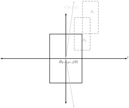
Figure 3. The boxes $B_{y}$ and $B_{z}$ are inside of $C(0,l,\alpha)$.

Therefore, fixing $y\in F_{m}$, it follows that

$$P_{y}[T^{l}_{2^{m+1}}<D^{\prime}(0)\mid\mathfrak{F}_{0,L}]\geq$$

$$\sum_{z\in\partial^{+}B_{y}}\mathbb{E}[P_{y,\omega}[X_{T_{B_{y}}}\in\partial^{+}B_{y},$$

$$X_{T_{B_{y}}}=z,(X_{T_{B_{z}}}\in\partial^{+}B_{z})\circ\theta_{T_{B_{y}}}]|\mathfrak{F}_{0,L}].$$ (72)

To estimate the right-hand side of the above inequality, it will be convenient to introduce the set

$$\bar{F}_{m}:=\partial[\cup_{y\in F_{m}}B_{y}]\cap\{R([2^{m-1}+2^{m},\infty)\times\mathbb{R}^{d-1})\},$$

and the event

$$G_{\bar{F}_{m}}:=\{\omega\in\Omega:\ P_{z,\omega}[X_{T_{B_{z}}}\in\partial^{+}B_{z}]>$$

$$1-2^{-\frac{M(m-1)}{2}},\ \mbox{for all }z\in\bar{F}_{m}\}.$$

Using the strong Markov property, we can now bound from below the right-hand side of inequality (72) by

$$(1-2^{-\frac{M(m-1)}{2}})\left(P_{y}[X_{T_{B_{y}}}\in\partial^{+}B_{y}|\mathfrak{F}_{0,L}]-P_{y}[(G_{\bar{F}_{m}})^{c}|\mathfrak{F}_{0,L}]\right).$$ (73)

In turn, by means of the polynomial condition and the fact that the boxes $B_{y}$ and $B_{z}$ are inside the cone $C(0,l,\alpha)$ we see that (73) is greater than or equal to

$$(1-2^{-\frac{M(m-1)}{2}})\left(1-2^{-M(m-1)}-P_{y}[(G_{\bar{F}_{m}})^{c}|\mathfrak{F}_{0,L}]\right).$$ (74)

Now, note that

$$P_{y}[(G_{\bar{F}_{m}})^{c}|\mathfrak{F}_{0,L}]\leq\sum_{x\in\bar{F}_{m}}2^{\frac{M(m-1)}{2}}P_{x}[X_{T_{B_{x}}}\not\in\partial^{+}B_{x}|\mathfrak{F}_{0,L}]$$

$$\leq|\bar{F}_{m}|2^{-\frac{M(m-1)}{2}}\leq(4c)^{d-1}2^{m(d-1)}2^{-\frac{M(m-1)}{2}}.$$ (75)

where in the first inequality we have used Chebyshev inequality, in the second one the assumption that $(PC)_{M,c}|_{l}$ is satisfied and in the third one the bound $|\bar{F}_{2m}|\leq(4c)^{d-1}2^{m(d-1)}$.

Consequently inserting the estimates (75) into (74) and combining this with inequality (72) we conclude that

$$P_{y}[T^{l}_{2^{m+1}}\leq D^{\prime}(0)\mid\mathfrak{F}_{0,L}]\geq\ (1-2^{-\frac{M(m-1)}{2}})\times$$

$$(1-2^{-\frac{M(m-1)}{2}}-(4c)^{d-1}2^{m(d-1)}2^{-\frac{M(m-1)}{2}})$$

$$\geq 1-3(4c)^{d-1}2^{m(d-1)}2^{-\frac{M(m-1)}{2}}.$$ (76)

Using the bound (76) in (71), together with the estimate $|F_{m}|\leq(2c)^{d-1}2^{m(d-1)}$, we see that

$$P_{0}[X_{T_{B_{2^{m},c2^{m},l}}(0)}\in\partial^{+}B_{2^{m},2^{m},l}(0),T^{l}_{2^{m+1}}\circ\theta_{T^{l}_{2^{m}}}>D^{\prime}(0)\circ\theta_{T^{l}_{2^{m}}}\mid\mathfrak{F}_{0,L}]$$

$$\leq 3(4c)^{2(d-1)}2^{2m(d-1)}2^{-\frac{M(m-1)}{2}}.$$ (77)

Combining the estimates (77), (70), (69) with (68) we conclude that

$$E_{0}[\mathfrak{M^{\prime}}^{2},D^{\prime}<\infty|\mathfrak{F}_{0,L}]$$

$$\leq 1+4(4c)^{2(d-1)}\sum_{m\geq 0}2^{2(m+1)}2^{2m(d-1)}2^{-\frac{M(m-1)}{2}}$$

$$\leq 1+4(4c)^{2(d-1)}\sum_{m\geq 0}2^{-m}\leq c_{6},$$

where in the second to last inequality we have used the fact that $M>4d+1$ and $c_{6}$ is a constant that does not depend on $L$. This completes the proof of the Lemma. ∎

5.3. Proof of Proposition 5.3

To simplify the computations, we introduce the notation

$$b=b(L):=P_{0}(D^{\prime}<\infty)+\phi(L),$$

$$b^{\prime}=b^{\prime}(L):=P_{0}(D^{\prime}=\infty)+\phi(L)$$

and $E_{\mathbb{P}\otimes Q}:=\mathbb{E}E_{Q}$. Furthermore, it will be necessary to define for each $j\geq 0$ and $n\geq L+j$ the events

$$D_{j,n}:=\{\varepsilon\in W^{\mathbb{N}}:(\varepsilon_{m},\ldots,\varepsilon_{m+L-1})\neq\overline{\varepsilon}^{(L)}\ {\rm for}\ {\rm all}\ j\leq m\leq j+n-L+1\}.$$

The following lemma, whose proof is presented in Appendix A, will be useful in the proof of Proposition 5.3.

Lemma 5.6.

There exists a constant $c_{7}$ such that for all $n\geq L^{2}$ one has that

$$Q[D_{0,n}]\leq(1-c_{7}L^{2}\kappa^{L})^{\left[\frac{n}{L^{2}}\right]}.$$

We now present the proof of Proposition 5.3, divided in several steps. For the sake of simplicity, we will write $\tau$ instead of $\tau^{(L)}$.

Step 0. We first note that

$$\bar{E}_{0}[(X_{\tau}\cdot u)^{2}\mid\mathfrak{F}_{0,L}]=$$

$$\displaystyle{\sum_{k=1}^{\infty}}\displaystyle{\sum_{k^{\prime}=0}^{k-1}}\bar{E}_{0}[(X_{S_{k^{\prime}+1}}\cdot u)^{2}-(X_{S_{k^{\prime}}}\cdot u)^{2},S_{k}<\infty,D^{\prime}\circ\theta_{S_{k}}=\infty\mid\mathfrak{F}_{0,L}].$$

(78)

Throughout the subsequent steps of the proof we will estimate the right-hand side of (78).

Step 1. Here we will prove the following estimate valid for all $k\geq 1$ and $0\leq k^{\prime}<k$.

$$\bar{E}_{0}[(X_{S_{k^{\prime}+1}}\cdot u)^{2}-(X_{S_{k^{\prime}}}\cdot u)^{2},S_{k}<\infty,D^{\prime}\circ\theta_{S_{k}}=\infty\mid\mathfrak{F}_{0,L}]$$

$$\leq b^{\prime}b^{k-k^{\prime}-1}\bar{E}_{0}[(X_{S_{k^{\prime}+1}}\cdot u)^{2}-(X_{S_{k^{\prime}}}\cdot u)^{2},S_{k^{\prime}+1}<\infty\mid\mathfrak{F}_{0,L}].$$ (79)

Furthermore, define the set

$$H^{L}:=\left\{y\in\mathbb{Z}^{d}:y\cdot u\geq L\frac{|u|_{2}}{|u|_{1}}\right\}.$$

Then, for each $0\leq k^{\prime}<k$, one has that

$$\bar{E}_{0}[(X_{S_{k^{\prime}+1}}\cdot u)^{2}-(X_{S_{k^{\prime}}}\cdot u)^{2},S_{k}<\infty,D^{\prime}\circ\theta_{S_{k}}=\infty\mid\mathfrak{F}_{0,L}]$$

$$\displaystyle{=\sum_{n\geq 1,x\in H^{L}}}E_{\mathbb{P}\otimes Q}[E_{\omega,\varepsilon}[(X_{S_{k^{\prime}+1}}\cdot u)^{2}-(X_{S_{k^{\prime}}}\cdot u)^{2},S_{k}=n,$$

$$X_{S_{k}}=x,D^{\prime}\circ\theta_{n}=\infty\mid\mathfrak{F}_{0,L}]$$

$$\displaystyle{=\sum_{n\geq 1,x\in H^{L}}}E_{\mathbb{P}\otimes Q}[E_{\omega,\varepsilon}[(X_{S_{k^{\prime}+1}}\cdot u)^{2}-(X_{S_{k^{\prime}}}\cdot u)^{2},S_{k}=n,X_{n}=x]$$

$$P_{\vartheta_{x}\omega,\ \theta_{n}\varepsilon}[D^{\prime}=\infty]\mid\mathfrak{F}_{0,L}]$$

$$\displaystyle{=\sum_{x\in H^{L}}}\mathbb{E}[\bar{E}_{0,\omega}[(X_{S_{k^{\prime}+1}}\cdot u)^{2}-(X_{S_{k^{\prime}}}\cdot u)^{2},S_{k}<\infty,X_{S_{k}}=x]$$

$$P_{x,\omega}[D^{\prime}=\infty]\mid\mathfrak{F}_{0,L}],$$

where here for each $x\in\mathbb{Z}^{d}$, $\vartheta_{x}$ denotes the canonical space shift in $\Omega$ so that $\vartheta_{x}\omega(y)=\omega(x+y)$, while for each $n\geq 0$, $\theta_{n}$ denotes the canonical time shift in the space $W$ so that $(\theta_{n}\epsilon)_{m}=\epsilon_{n+m}$, in the first equality we have used the fact that the value of $X_{S_{k}}\cdot u\geq X_{S_{1}}\cdot u$, in the second equality the Markov property and in the last equality we have used the independence of the coordinates of $\epsilon$ and the fact that the law of the random walk is the same under $P_{x,\omega}$ and under $E_{Q}P_{\vartheta_{x}\omega,\theta_{n}\epsilon}$.

Moreover, by the fact that the first factor inside the expectation of the right-most expression of (5.3) is $\mathfrak{F}_{x,L}$-measurable, the right-most expression in (5.3) is equal to

$$\displaystyle{\sum_{x\in H^{L}}}\mathbb{E}[\bar{E}_{0,\omega}[(X_{S_{k^{\prime}+1}}\cdot u)^{2}-(X_{S_{k^{\prime}}}\cdot u)^{2},S_{k}<\infty,X_{S_{k}}=x]$$

$$\mathbb{E}[P_{x,\omega}[D^{\prime}=\infty]\mid\mathfrak{F}_{x,L}]\mid\mathfrak{F}_{0,L}].$$ (81)

Applying next Lemma 5.4 to (81), we see that

$$\sum_{x\in H^{L}}\mathbb{E}[\bar{E}_{0,\omega}[(X_{S_{k^{\prime}+1}}\cdot u)^{2}-(X_{S_{k^{\prime}}}\cdot u)^{2},S_{k}<\infty,X_{S_{k}}=x]$$

$$\times\mathbb{E}[P_{x,\omega}[D^{\prime}=\infty]\mid\mathfrak{F}_{x,L}]\mid\mathfrak{F}_{0,L}]$$

$$\leq b^{\prime}\bar{E}_{0}[(X_{S_{k^{\prime}+1}}\cdot u)^{2}-(X_{S_{k^{\prime}}}\cdot u)^{2},S_{k}<\infty\mid\mathfrak{F}_{0,L}].$$ (82)

Next, observe that for $k^{\prime}<k$ one has that

$$\bar{E}_{0}[(X_{S_{k^{\prime}+1}}\cdot u)^{2}-(X_{S_{k^{\prime}}}\cdot u)^{2},S_{k}<\infty\mid\mathfrak{F}_{0,L}]$$

$$=\bar{E}_{0}[(X_{S_{k^{\prime}+1}}\cdot u)^{2}-(X_{S_{k^{\prime}}}\cdot u)^{2},R_{k-1}<\infty\mid\mathfrak{F}_{0,L}]$$

$$=\sum_{x\in H^{L}}\mathbb{E}[\bar{E}_{0,\omega}[(X_{S_{k^{\prime}+1}}\cdot u)^{2}-(X_{S_{k^{\prime}}}\cdot u)^{2},S_{k-1}<\infty,X_{S_{k-1}}=x,$$

$$D^{\prime}\circ\theta_{S_{k-1}}<\infty]\mid\mathfrak{F}_{0,L}]$$

$$=\sum_{x\in H^{L}}\mathbb{E}[\bar{E}_{0,\omega}[(X_{S_{k^{\prime}+1}}\cdot u)^{2}-(X_{S_{k^{\prime}}}\cdot u)^{2},S_{k-1}<\infty,X_{S_{k-1}}=x]$$

$$P_{x,\omega}[D^{\prime}<\infty]\mid\mathfrak{F}_{0,L}]$$

$$=\sum_{x\in H^{L}}\mathbb{E}[\bar{E}_{0,\omega}[(X_{S_{k^{\prime}+1}}\cdot u)^{2}-(X_{S_{k^{\prime}}}\cdot u)^{2},S_{k-1}<\infty,X_{S_{k-1}}=x]$$

$$\mathbb{E}[P_{x,\omega}[D^{\prime}<\infty]\mid\mathfrak{F}_{x,L}]\mid\mathfrak{F}_{0,L}].$$ (83)

By Lemma 5.4, we have that $\mathbb{E}[P_{x,\omega}[D^{\prime}<\infty]\mid\mathfrak{F}_{x,L}]\leq b=P_{0}[D^{\prime}<\infty]+\phi(L)$. Using this inequality to estimate the last term in (83), we see that

$$\bar{E}_{0}[(X_{S_{k^{\prime}+1}}\cdot u)^{2}-(X_{S_{k^{\prime}}}\cdot u)^{2},S_{k}<\infty\mid\mathfrak{F}_{0,L}]$$

$$\leq b\bar{E}_{0}[(X_{S_{k^{\prime}+1}}\cdot u)^{2}-(X_{S_{k^{\prime}}}\cdot u)^{2},S_{k-1}<\infty\mid\mathfrak{F}_{0,L}].$$

By induction on $k$ we get that

$$\bar{E}_{0}[(X_{S_{k^{\prime}+1}}\cdot u)^{2}-(X_{S_{k^{\prime}}}\cdot u)^{2},S_{k}<\infty\mid\mathfrak{F}_{0,L}]$$

$$\leq b^{k-k^{\prime}-1}\bar{E}_{0}[(X_{S_{k^{\prime}+1}}\cdot u)^{2}-(X_{S_{k^{\prime}}}\cdot u)^{2},S_{k^{\prime}+1}<\infty\mid\mathfrak{F}_{0,L}].$$ (84)

Combining (84) with (82) we obtain (79).

Step 2. For $k\geq 1$ we define

$$M_{k}:=\sup_{0\leq n\leq R_{k}}X_{n}\cdot u.$$ (85)

Define also the sets parametrized by $k$ and $n\geq 0$

$$A_{n,k}:=\left\{\varepsilon\in W^{\mathbb{N}}:\left(\varepsilon_{t^{(n)}_{k}},\varepsilon_{t^{(n)}_{k}+1},\ldots,\varepsilon_{t^{(n)}_{k}+L-1}\right)=\overline{\varepsilon}^{(L)}\right\}$$ (86)

and

$$B_{n,k}:=\left\{\varepsilon\in W^{\mathbb{N}}:\left(\varepsilon_{t^{(j)}_{k}},\varepsilon_{t^{(j)}_{k}+1},\ldots,\varepsilon_{t^{(j)}_{k}+L-1}\right)\neq\overline{\varepsilon}^{(L)}\ {\rm for}\ {\rm all}\ 0\leq j\leq n-1\right\},$$ (87)

where we define the sequence of stopping times [c.f. (66)] parameterized by $k$ and recursively on $n\geq 0$ by

$$t^{(0)}_{k}:=\bar{T}^{l}_{M_{k}}$$

and the successive times where a record value of the projection of the random walk on $l$ is achieved by

$$t_{k}^{(n+1)}:=\bar{T}^{l}_{X_{t_{k}^{(n)}}\cdot u}.$$

In this step we will show that for all $k\geq 0$ one has that

$$\bar{E}_{0}[(X_{S_{k+1}}\cdot u)^{2}-(X_{S_{k}}\cdot u)^{2},S_{k+1}<\infty|\mathfrak{F}_{0,L}]$$

$$\leq\sum_{n=0}^{L^{2}-1}\bar{E}_{0}[(X_{S_{k+1}}\cdot u)^{2}-(X_{S_{k}}\cdot u)^{2},t^{(n)}_{k}<\infty,A_{n,k}\mid\mathfrak{F}_{0,L}]$$

$$\!\!+\sum_{n=L^{2}}^{\infty}\bar{E}_{0}[(X_{S_{k+1}}\cdot u)^{2}-(X_{S_{k}}\cdot u)^{2},t^{(n)}_{k}<\infty,B_{n,k},A_{n,k}\mid\mathfrak{F}_{0,L}],$$ (88)

To prove (88), we have to introduce some further notations. Now, note that on the event $A_{n,k}\cap B_{n,k}$ one has that

$$S_{k+1}=t^{(n)}_{k}+L.$$

Thus, as a consequence of the definition of $S_{k+1}$, one has that $\bar{P}_{0}$-a.s.

$$\{S_{k+1}<\infty\}\subset\bigcup_{n\geq 0}\{t^{(n)}_{k}<\infty,B_{n,k},A_{n,k}\}.$$ (89)

Display (88) now follows directly from (89).

Step 3. Here we will derive an upper bound for the two sums appearing in the right-hand side in (88). In fact, we will prove that there is a constant $c_{8}$ such that for all $k\geq 1$ one has that

$$\sum_{n=0}^{L^{2}-1}\bar{E}_{0}[(X_{S_{k+1}}\cdot u)^{2}-(X_{S_{k}}\cdot u)^{2},t^{(n)}_{k}<\infty,A_{n,k}\mid\mathfrak{F}_{0,L}]$$

$$\leq c_{8}\kappa^{L}\left(L^{4}b^{k-1}+L^{2}\bar{E}_{0}[X_{S_{k}}\cdot u,S_{k}<\infty|\mathfrak{F}_{0,L}]\right)$$ (90)

and

$$\sum_{n=L^{2}}^{\infty}\bar{E}_{0}[(X_{S_{k+1}}\cdot u)^{2}-(X_{S_{k}}\cdot u)^{2},t^{(n)}_{k}<\infty,B_{n,k},A_{n.k}\mid\mathfrak{F}_{0,L}]$$

$$\leq c_{8}\sum_{n=L^{2}}^{\infty}\kappa^{L}(1-c_{7}\kappa^{L})^{\left[\frac{n}{L^{2}}\right]}\left((n+L)^{2}b^{k-1}\right.$$

$$\left.+(n+L)\bar{E}_{0}[X_{S_{k}}\cdot u,S_{k}<\infty|\mathfrak{F}_{0,L}]\right).$$ (91)

Note that for all $n\geq 0$ one has that

$$X_{t^{(n+1)}_{k}}\cdot u\leq X_{t^{(n)}_{k}}\cdot u+|u|_{\infty},$$

and hence by induction on $n$ we get that

$$X_{t^{(n)}_{k}}\cdot u\leq M_{k}+(n+1)|u|_{\infty}.$$

Therefore, if we set

$$L^{\prime}:=\frac{L|u|}{|u|_{1}}+|u|_{\infty}\leq c_{9}L,$$ (92)

where $c_{9}$ is a constant depending on $l$ and $d$, we can see that $P_{0}$-a.s on the event $\{t^{(n)}_{k}<\infty,\ A_{n,k}\}$ one has that

$$X_{S_{k+1}}\cdot u\leq N_{k,n}:=M_{k}+n|u|_{\infty}+L^{\prime}.$$ (93)

Therefore, for all $0\leq n\leq L^{2}-1$ one has that

$$\bar{E}_{0}[(X_{S_{k+1}}\cdot u)^{2}-(X_{S_{k}}\cdot u)^{2},t^{(n)}_{k}<\infty,A_{n,k}\mid\mathfrak{F}_{0,L}]$$

$$\leq\bar{E}_{0}[N_{k,n}^{2}-(X_{S_{k}}\cdot u)^{2},t^{(n)}_{k}<\infty,A_{n,k}\mid\mathfrak{F}_{0,L}]$$

$$=\sum_{j=0}^{\infty}\sum_{x\in\mathbb{Z}^{d}}E_{\mathbb{P}\otimes Q}[E_{\omega,\varepsilon}[N_{k,n}^{2}-(X_{S_{k}}\cdot u)^{2},$$

$$t^{(n)}_{k}=j,X_{j}=x]\mathds{1}_{\{(\varepsilon_{j},\ldots,\varepsilon_{j+L-1})=\overline{\varepsilon}^{(L)}\}}\mid\mathfrak{F}_{0,L}]$$

$$\leq\kappa^{L}\bar{E}_{0}[N_{k,n}^{2}-(X_{S_{k}}\cdot u)^{2},R_{k}<\infty\mid\mathfrak{F}_{0,L}],$$ (94)

where in the equality we have applied the Markov property and in the second inequality the fact that $Q$ is a product measure and that $R_{k}\leq t^{(n)}_{k}$. Similarly for all $n\geq L^{2}$ one has that

$$\bar{E}_{0}[(X_{S_{k+1}}\cdot u)^{2}-(X_{S_{k}}\cdot u)^{2},t^{(n)}_{k}<\infty,B_{n,k},A_{n,k}\mid\mathfrak{F}_{0,L}]$$

$$\leq\bar{E}_{0}[N_{k,n}^{2}-(X_{S_{k}}\cdot u)^{2},t^{(n)}_{k}<\infty,B_{n,k},A_{n,k}\mid\mathfrak{F}_{0,L}]$$

$$\leq\sum_{j=0}^{\infty}\sum_{j^{\prime}=j+n}^{\infty}\sum_{y\in\mathbb{Z}^{d}}E_{\mathbb{P}\otimes Q}\ [E_{\omega,\varepsilon}[N_{k,n}^{2}-(X_{S_{k}}\cdot u)^{2},$$

$$X_{t^{(0)}_{k}}=y,t^{(0)}_{k}=j]P_{\theta_{y}\omega,\theta_{j}\varepsilon}[D_{j,n},t^{(n)}_{k}=j^{\prime}]\mathds{1}_{\{(\varepsilon_{j^{\prime}},\ldots,\varepsilon_{j^{\prime}+L-1})=\overline{\varepsilon}^{(L)}\}}]\mid\mathfrak{F}_{0,L}]$$

$$\leq\kappa^{L}Q[D_{0,n}]\bar{E}_{0}[N_{k,n}^{2}-(X_{S_{k}}\cdot u)^{2},R_{k}<\infty\mid\mathfrak{F}_{0,L}]$$

$$\leq\kappa^{L}(1-c_{7}L^{2}\kappa^{L})^{\left[\frac{n}{L}\right]}\bar{E}_{0}[N_{k,n}^{2}-(X_{S_{k}}\cdot u)^{2},R_{k}<\infty\mid\mathfrak{F}_{0,L}],$$ (95)

where in the second inequality we have used the Markov property, in the third one the fact that $R_{k}\leq t_{k}^{(0)}$ and in the last one Lemma 5.6.

Now, by displays (94) and (95), to finish the proof of inequalities (90) and (91) it is enough to prove that there is a constant $c_{10}$ such that

$$\bar{E}_{0}[N_{k,n}^{2}-(X_{S_{k}}\cdot u)^{2},R_{k}<\infty\mid\mathfrak{F}_{0,L}]$$

$$\leq c_{10}\left((n+L)^{2}b^{k-1}+(n+L)\bar{E}_{0}[X_{S_{k}}\cdot u,S_{k}<\infty|\mathfrak{F}_{0,L}]\right),$$ (96)

using the fact that $n\leq L^{2}-1$ in the left-hand side of inequality (90). To prove (96), the following identity will be useful

$$N_{k,n}^{2}-(X_{S_{k}}\cdot u)^{2}=(M_{k}-X_{S_{k}}\cdot u)^{2}$$

$$+2(n|u|_{\infty}+L^{\prime})(M_{k}-X_{S_{k}}\cdot u)+2(n|u|_{\infty}+L^{\prime})X_{S_{k}}\cdot u$$

$$+2(M_{k}-X_{S_{k}}\cdot u)X_{S_{k}}\cdot u+(n|u|_{\infty}+L^{\prime})^{2}.$$ (97)

We will now insert this decomposition in the left-hand side of (96) and bound the corresponding expectations of each term. Let us begin with the expectation of the last term. Note that by an argument similar to the one developed in Step 1 we have that

$$\bar{E}_{0}[(n|u|_{\infty}+L^{\prime})^{2},R_{k}<\infty|\mathfrak{F}_{0,L}]\leq c_{11}(n+L)^{2}b^{k},$$ (98)

for some constant $c_{11}$. Similarly, the expectation of the first term of the right-hand side of display (97) can be bounded using Lemma 5.5, so that

$$\bar{E}_{0}[(M_{k}-X_{S_{k}}\cdot u)^{2},R_{k}<\infty\mid\mathfrak{F}_{0,L}]$$

$$=\displaystyle{\sum_{x\in H^{L}}}\mathbb{E}[\bar{P}_{0,\omega}[S_{k}<\infty,X_{S_{k}}=x]E_{x}[\mathfrak{M}^{2},D^{\prime}<\infty\mid\mathfrak{F}_{x,L}]\mid\mathfrak{F}_{0,L}]$$

$$\leq c_{6}b^{k-1}.$$ (99)

Again, for the expectation of the second term of the right-hand side of display (97), we have that

$$\bar{E}_{0}[2(n|u|_{\infty}+L^{\prime})(M_{k}-X_{S_{k}}\cdot u),R_{k}<\infty\mid\mathfrak{F}_{0,L}]$$

$$\leq c_{12}b^{k-1}(n+L),$$ (100)

for some suitable positive constant $c_{12}$. For the expectation of fourth term of the right-hand side of (97), we see by Lemma 5.5 that

$$\bar{E}_{0}[2(M_{k}-X_{S_{k}}\cdot u)X_{S_{k}}\cdot u,R_{k}<\infty\mid\mathfrak{F}_{0,L}]$$

$$\leq 2\sqrt{c_{6}}\bar{E}_{0}[X_{S_{k}}\cdot u,S_{k}<\infty\mid\mathfrak{F}_{0,L}].$$ (101)

Finally, for the expectation of third term of the right-hand side of (97) we have that

$$\bar{E}_{0}[2(n|u|_{\infty}+L^{\prime})X_{S_{k}}\cdot u,R_{k}<\infty\mid\mathfrak{F}_{0,L}]$$

$$\leq c_{12}b(n+L)\bar{E}_{0}[X_{S_{k}}\cdot u,S_{k}<\infty\mid\mathfrak{F}_{0,L}].$$ (102)

Using the bounds (102), (101), (100), (99) and (98) we obtain inequality (96).

Step 4. Here we will derive for all $k\geq 1$ the inequality

$$\bar{E}_{0}[X_{S_{k}}\cdot u,S_{k}<\infty|\mathfrak{F}_{0,L}]$$

$$\leq\sum_{k^{\prime}=0}^{k-1}b^{k-k^{\prime}-1}\left(\sum_{n=0}^{L^{2}-1}\,\bar{E}_{0}[N_{k^{\prime},n}-X_{S_{k^{\prime}}}\cdot u,t^{(n)}_{k^{\prime}}<\infty,A_{n,k^{\prime}}\mid\mathfrak{F}_{0,L}]+\right.$$

$$\!\!\!\!\!\left.\sum_{n=L^{2}}^{\infty}\,\bar{E}_{0}[N_{k^{\prime},n}-X_{S_{k^{\prime}}}\cdot u,t^{(n)}_{k^{\prime}}<\infty,B_{n,k^{\prime}},A_{n,k^{\prime}}\mid\mathfrak{F}_{0,L}]\right).$$ (103)

Note that

$$\bar{E}_{0}[X_{S_{k}}\cdot u,S_{k}<\infty\mid\mathfrak{F}_{0,L}]$$

$$=\sum_{k^{\prime}=0}^{k-1}\bar{E}_{0}[(X_{S_{k^{\prime}+1}}-X_{S_{k^{\prime}}})\cdot u,S_{k}<\infty\mid\mathfrak{F}_{0,L}].$$ (104)

By an argument similar to the one used in Step 1 we see that for $k^{\prime}<k$ one has that

$$\bar{E}_{0}[(X_{S_{k^{\prime}+1}}-X_{S_{k}^{\prime}})\cdot u,S_{k}<\infty\mid\mathfrak{F}_{0,L}]$$

$$\leq b^{k-k^{\prime}-1}\bar{E}_{0}[(X_{S_{k^{\prime}+1}}-X_{S_{k}^{\prime}})\cdot u,S_{k^{\prime}+1}<\infty\mid\mathfrak{F}_{0,L}].$$ (105)

Now, we can use inclusion (89) in order to get that

$$\bar{E}_{0}[(X_{S_{k^{\prime}+1}}-X_{S_{k}^{\prime}})\cdot u,S_{k^{\prime}+1}<\infty\mid\mathfrak{F}_{0,L}]$$

$$\leq\sum_{n=0}^{L^{2}-1}\,\bar{E}_{0}[(X_{S_{k^{\prime}+1}}-X_{S_{k}^{\prime}})\cdot u,t^{(n)}_{k^{\prime}}<\infty,B_{n,k^{\prime}},A_{n,k^{\prime}}\mid\mathfrak{F}_{0,L}]$$

$$+\sum_{n=L^{2}}^{\infty}\,\bar{E}_{0}[(X_{S_{k^{\prime}+1}}-X_{S_{k}^{\prime}})\cdot u,t^{(n)}_{k^{\prime}}<\infty,B_{n,k^{\prime}},A_{n,k^{\prime}}\mid\mathfrak{F}_{0,L}],$$ (106)

where the events $A_{n,k^{\prime}}$ and $B_{n,k^{\prime}}$ are defined in (86) and (87). Using the fact that on the event $\{t^{(n)}_{k^{\prime}}<\infty,B_{n,k^{\prime}},A_{n,k^{\prime}}\}$ one has that $P_{0}$-a.s.

$$(X_{S_{k^{\prime}+1}}-X_{S_{k^{\prime}}})\cdot u\leq N_{k^{\prime},n}-X_{S_{k}^{\prime}}\cdot u,$$

we see that the right-hand side of (106) is bounded by the right-hand side of (103), which is what we want to prove.

Step 5. Here we will obtain an upper bound for the terms in the first summation in (106). Indeed, note that on $R_{k^{\prime}}\leq t^{(n)}_{k^{\prime}}$, by an argument similar to the one used to derive inequality (94), we have that for all $0\leq n\leq L^{2}$ and $0\leq k^{\prime}\leq k-1$

$$\bar{E}_{0}[N_{k^{\prime},n}-X_{S_{k^{\prime}}}\cdot u,t^{(n)}_{k^{\prime}}<\infty,A_{n,k^{\prime}}\mid\mathfrak{F}_{0,L}]$$

$$\leq\kappa^{L}\bar{E}_{0}[N_{k^{\prime},n}-X_{S_{k^{\prime}}}\cdot u,R_{k^{\prime}}<\infty\mid\mathfrak{F}_{0,L}].$$

Step 6. Here we will obtain an upper bound for the terms in the second summation in (106), showing that for all $n\geq L^{2}$ and $0\leq k^{\prime}\leq k-1$,

$$E_{0}[N_{k^{\prime},n}-X_{S_{k^{\prime}}}\cdot u,t^{(n)}_{k^{\prime}}<\infty,B_{n,k^{\prime}},A_{n,k^{\prime}}\mid\mathfrak{F}_{0,L}]$$

$$\leq\kappa^{L}\left(1-c_{7}L^{2}\kappa^{L}\right)^{\left[\frac{n}{L}\right]}\bar{E}_{0}[N_{k^{\prime},n}-X_{S_{k^{\prime}}}\cdot u,R_{k^{\prime}}<\infty\mid\mathfrak{F}_{0,L}].$$ (107)

Now note that

$$E_{0}[N_{k^{\prime},n}-X_{S_{k^{\prime}}}\cdot u,t^{(n)}_{k^{\prime}}<\infty,B_{n,k^{\prime}},A_{n,k^{\prime}}\mid\mathfrak{F}_{0,L}]$$

$$\leq\sum_{j=0}^{\infty}\sum_{j^{\prime}\geq j+n}\sum_{y\in\mathbb{Z}^{d}}E_{\mathbb{P}\otimes Q}\ [E_{\omega,\varepsilon}[N_{k^{\prime},n}-X_{S_{k^{\prime}}}\cdot u,$$

$$X_{t^{(0)}_{k^{\prime}}}=y,t^{(0)}_{k^{\prime}}=j]P_{\theta_{y}\omega,\theta_{j}\varepsilon}[D_{j,n},t^{(n)}_{k^{\prime}}=j^{\prime}]\mathds{1}_{\{(\varepsilon_{j^{\prime}},\ldots,\varepsilon_{j^{\prime}+L-1})=\overline{\varepsilon}^{(L)}\}}]\mid\mathfrak{F}_{0,L}]$$

$$=\kappa^{L}Q[D_{0,n}]\mathbb{E}[\bar{E}_{0,\omega}[N_{k^{\prime},n}-X_{S_{k^{\prime}}}\cdot u,t^{(0)}_{k^{\prime}}<\infty]\mid\mathfrak{F}_{0,L}].$$

Using Lemma 5.6 to estimate $Q[D_{0,n}]$ we conclude the proof of inequality (107).

Step 7. Here we will show that there exist constant $c_{13}$ and $c_{14}$ such that

$$\sum_{n=0}^{L^{2}-1}\bar{E}_{0}[N_{k^{\prime},n}-X_{S_{k^{\prime}}}\cdot u,t^{(n)}_{k^{\prime}}<\infty,A_{n,k^{\prime}}\mid\mathfrak{F}_{0,L}]\leq c_{13}\kappa^{L}L^{4}b^{k^{\prime}-1}$$ (108)

and

$$\sum_{n=L^{2}}^{\infty}\bar{E}_{0}[N_{k^{\prime},n}-X_{S_{k^{\prime}}}\cdot u,t^{(n)}_{k^{\prime}}<\infty,A_{n,k^{\prime}},B_{n,k^{\prime}}\mid\mathfrak{F}_{0,L}]\\ \leq 4c_{14}\kappa^{-L}b^{k^{\prime}-1}.$$ (109)

Let us first note that by an argument similar to the one used to derive the bound in Step 1 (through Lemmas 5.4 and 5.5), we have that

$$\bar{E}_{0}[N_{k^{\prime},n}-X_{S_{k}^{\prime}}\cdot u,R_{k^{\prime}}<\infty]\\ \leq(n|u|_{\infty}+L^{\prime}+c_{15})b^{k^{\prime}-1},$$ (110)

where $c_{15}:=\sqrt{c_{6}}$. Let us now prove (108). Indeed, note that by Step 5 and (110) we then have that

$$\sum_{n=0}^{L^{2}-1}\bar{E}_{0}[N_{k^{\prime},n}-X_{S_{k^{\prime}}}\cdot u,t^{(n)}_{k^{\prime}}<\infty,A_{n,k^{\prime}}\mid\mathfrak{F}_{0,L}]$$

$$\leq\kappa^{L}\sum_{n=0}^{L^{2}-1}\bar{E}_{0}[N_{k^{\prime},n}-X_{S_{k^{\prime}}}\cdot u,R_{k^{\prime}}<\infty\mid\mathfrak{F}_{0,L}]$$

$$\leq c_{13}\ L^{4}\ \kappa^{L}b^{k^{\prime}-1},$$ (111)

for some suitable constant $c_{13}$. Let us now prove (109). First note that

$$\sum_{n=L^{2}}^{\infty}\bar{E}_{0}[N_{k^{\prime},n}-X_{S_{k^{\prime}}}\cdot u,t^{(n)}_{k^{\prime}}<\infty,A_{n,k^{\prime}},B_{n,k^{\prime}}\mid\mathfrak{F}_{0,L}]$$

$$\leq\sum_{n=L^{2}}^{\infty}\kappa^{L}(1-c_{7}L^{2}\kappa^{L})^{\left[\frac{n}{L}\right]}\bar{E}_{0}[N_{k^{\prime},n}-X_{S_{k^{\prime}}}\cdot u,R_{k^{\prime}}<\infty\mid\mathfrak{F}_{0,L}]$$

$$\leq b^{k^{\prime}-1}\sum_{n=L^{2}}^{\infty}\kappa^{L}(1-c_{7}L^{2}\kappa^{L})^{\left[\frac{n}{L}\right]}(n|u|_{\infty}+L^{\prime}+c_{15})$$

$$\leq c_{16}b^{k^{\prime}-1}\sum_{n=L^{2}}^{\infty}n\kappa^{L}(1-c_{33}L^{2}\kappa^{L})^{[\frac{n}{L^{2}}]}.$$ (112)

for some constant $c_{16}$, where in the first inequality we have used Step 6 and in the second we have used inequality (110). Finally notice that using the fact that for $n\geq L^{2}$ one has that $n\leq 2L^{2}\left[\frac{n}{L^{2}}\right]$, we get that

$$\sum_{n=L^{2}}^{\infty}n\kappa^{L}(1-c_{7}L^{2}\kappa^{L})^{\left[\frac{n}{L^{2}}\right]}\leq 2\kappa^{L}L^{2}\sum_{n=L^{2}}^{\infty}\left[\frac{n}{L^{2}}\right](1-c_{7}L^{2}\kappa^{L})^{\left[\frac{n}{L^{2}}\right]}$$

$$=2L^{4}\kappa^{L}\sum_{m=1}^{\infty}m(1-c_{7}L^{2}\kappa^{L})^{m}\leq\frac{2}{(c_{7})^{2}}\kappa^{-L}.$$

Using this estimate in (112) we obtain (109).

Step 8. Here we finish the proof of Proposition 5.3 combining the previous steps we have already developed. Combining inequality (103) proved in Step 4 with inequalities (108) and (109) proved in Step 7, we see that there is a constant $c_{17}$ such that

$$\bar{E}_{0}[X_{S_{k}}\cdot u,S_{k}<\infty\mid\mathfrak{F}_{0,L}]\leq c_{17}kb^{k-2}\kappa^{-L}.$$ (113)

Thus, by inequality (90) proved in Step 3, we have that

$$\sum_{n=0}^{L^{2}-1}\bar{E}_{0}[(X_{S_{k+1}}\cdot u)^{2}-(X_{S_{k}}\cdot u)^{2},t^{(n)}_{k}<\infty,A_{n,k}\mid\mathfrak{F}_{0,L}]\leq c_{18}L^{4}kb^{k-2}.$$ (114)

for certain positive constant $c_{18}$ On the other hand, combining inequality (91) proved in Step 3 with (113), we see that there exists a constant $c_{19}$ such that

$$\sum_{n=L^{2}}^{\infty}\bar{E}_{0}[(X_{S_{k+1}}\cdot u)^{2}-(X_{S_{k}}\cdot u)^{2},t^{(n)}_{k}<\infty,B_{n,k},A_{n,k}\mid\mathfrak{F}_{0,L}]$$

$$\leq c_{19}\sum_{n=L^{2}}^{\infty}\kappa^{L}(1-c_{7}L^{2}\kappa^{L})^{\left[\frac{n}{L^{2}}\right]}\left((n+L)^{2}b^{k-1}\right.$$

$$\left.+(n+L)kb^{k-2}\kappa^{-L}\right).$$ (115)

Now, note that for some constant $c_{20}$ one has that

$$\sum_{n=L^{2}}^{\infty}(n+L)^{2}(1-c_{7}L^{2}\kappa^{L})^{[\frac{n}{L^{2}}]}\leq c_{20}\ \kappa^{-3L}\quad{\rm and}$$ (116)

$$\sum_{n=L^{2}}^{\infty}(n+L)(1-c_{7}L^{2}\kappa^{L})^{[\frac{n}{L^{2}}]}\leq c_{20}\ \kappa^{-2L}.$$ (117)

Substituting (116) and (117) into (115) we see that

$$\sum_{n=L^{2}}^{\infty}\bar{E}_{0}[(X_{S_{k+1}}\cdot u)^{2}-(X_{S_{k}}\cdot u)^{2},t^{(n)}_{k}<\infty,B_{n,k},A_{n,k}\mid\mathfrak{F}_{0,L}]\leq$$

$$c_{21}\kappa^{-2L}b^{k-2}k,$$ (118)

for some suitable positive constant $c_{21}$. Substituting (115) and (118) into inequality (88) of Step 2, we then conclude that there is a constant $c_{22}$ such that

$$\bar{E}_{0}[(X_{S_{k+1}}\cdot u)^{2}-(X_{S_{k}}\cdot u)^{2},S_{k+1}<\infty|\mathfrak{F}_{0,L}]\leq c_{22}\kappa^{-2L}b^{k-2}k.$$ (119)

Substituting (119) into (79) of Step 1, we get that

$$\bar{E}_{0}[(X_{S_{k^{\prime}+1}}\cdot u)^{2}-(X_{S_{k^{\prime}}}\cdot u)^{2},S_{k}<\infty,D^{\prime}\circ\theta_{S_{k}}=\infty\mid\mathfrak{F}_{0,L}]$$

$$\leq b^{\prime}b^{k+1}k^{\prime}.$$ (120)

From the fact that $\sum_{k=1}^{\infty}\sum_{k^{\prime}=0}^{k-1}b^{k+1}k^{\prime}<\infty$ together with (120 and (78) of Step 0, we conclude that

$$\bar{E}_{0}[(X_{\tau}\cdot u)^{2}|\mathfrak{F}_{0,L}]\leq c_{23}\kappa^{-2L},$$

for some constant $c_{23}>0$, which proves the proposition.

6. Proof of Theorem 1.1

In this section we will prove Theorem 1.1 using Proposition 5.3 proved in Section 5. First in Subsection 6.1, we will define an approximate sequence of regeneration times. In Subsection 6.2, we will show through this approximate regeneration time sequence, that there exists an approximate asymptotic direction. In Subsection 6.3, we will use the approximate asymptotic direction to prove Theorem 1.1.

6.1. Approximate regeneration time sequence

As in [CZ01], we define approximate regeneration by the recursively by $\tau_{1}^{(L)}:=\tau$ [c.f.(58)] and for $i\geq 2$

$$\tau_{i}^{(L)}:=\tau_{1}^{(L)}\circ\theta_{\tau_{i-1}^{(L)}}+\tau_{i-1}^{(L)}.$$

We will drop the dependence in $L$ on $\tau_{1}^{(L)}$ when it is convenient for us, using the notation $\tau_{i}$ instead $\tau_{i}^{(L)}$. Let us define $\sigma$-algebras corresponding to the information of the random walk and the $\varepsilon$ process up to the first regeneration time and of the environment $\omega$ at a distance of order $L$ to the left of the position of the random walk at this regeneration time as

$$\mathcal{H}_{1}:=\sigma(\tau_{1}^{(L)},X_{0},\varepsilon_{0},\ldots,\varepsilon_{\tau_{1}^{(L)}-1},X_{\tau_{1}^{(L)}},$$

$$\{\omega(y,\cdot):\ y\cdot u<u\cdot X_{\tau_{1}^{(L)}}-L|u|/|u|_{1}\}).$$

Similarly define for $k\geq 2$

$$\mathcal{H}_{k}:=\sigma(\tau_{1}^{(L)},\ldots,\tau_{k}^{(L)},X_{0},\varepsilon_{0},\ldots,\varepsilon_{\tau_{k}^{(L)}-1},X_{\tau_{k}^{(L)}},$$

$$\{\omega(y,\cdot):\ y\cdot u<u\cdot X_{\tau_{k}^{(L)}}-L|u|/|u|_{1}\}).$$ (121)

Let us now recall Lemma 2.3 of [CZ01], stated here under the condition $P_{0}[D^{\prime}=\infty]>0$ [c.f. (32)] instead of Kalikow’s condition.

Lemma 6.1.

Let $l\in\mathbb{S^{*}}^{d-1}$, $\alpha>0$ and $\phi$ be such that $\lim_{r\to\infty}\phi(r)=0$. Consider a random walk in a random environment satisfying the cone-mixing assumption with respect to $\alpha$, $l$ and $\phi$ and uniformly elliptic with respect to $l$. Assume that $L$ is such that

$$\phi(L)<P_{0}[D^{\prime}=\infty].$$

Then, $\mathbb{P}-$a.s. one has that

$$\left|\bar{P}_{0}[\{X_{\tau_{k}+\cdot}-X_{\tau_{k}}\}\in A\mid\mathcal{H}_{k}]-\bar{P}_{0}[\{X_{\cdot}\}\in A|D^{\prime}=\infty]\right|\leq\phi^{\prime}(L),$$

for all measurable sets $A\subset\mathbb{(}\mathbb{Z}^{d})^{\mathbb{N}}$, where

$$\phi^{\prime}(L):=\frac{2\phi(L)}{(P_{0}[D^{\prime}=\infty]-\phi(L))}.$$

Proof.

For $k=1$, the argument given in page 890 of ([CZ01]) still works without any change. With the purpose of showing that the result continues being true under the weaker assumptions here, we complete the induction argument in the case $k=2$. To this end, we consider a positive $\mathcal{H}_{2}-$ measurable function $h$ of the form $h=h_{1}\cdot(h_{2})\circ\theta_{\tau_{1}}$ ($\cdot$ denotes usual function multiplication), such that $h_{1},$ is $\mathcal{H}_{1}-$ measurable and $h_{2}$ is $\mathcal{H^{\prime}}_{1}$ measurable, where the $\sigma-$ algebra $\mathcal{H^{\prime}}_{1}$ is defined as :

$$\mathcal{H^{\prime}}_{1}: = \sigma(\tau_{1}^{(L)},X_{0},\varepsilon_{0},\ldots,\varepsilon_{\tau_{1}^{(L)}-1},X_{\tau_{1}^{(L)}},$$

$$\{\omega(y,\cdot):\ u\cdot y\leq u\cdot X_{\tau_{1}^{(L)}}-L\frac{|u|}{|u|_{1}},\ y\in C(X_{0},l,\alpha)\}).$$

We let $A$ be a measurable set of the path space, for short we will write $\mathds{1}_{A}:=\mathds{1}_{\{(X_{n}-X_{0})_{n\geq 0}\in A\}}$. By the strong Markov property and using that $\tau_{1}<\infty$ within an event of full $P_{0}$ probability, we get:

$$\displaystyle{\bar{E}_{0}[h\mathds{1}_{A}\circ\theta_{\tau_{2}}]\leq\sum_{n\geq 1}E_{0}[h\mathds{1}_{A}\circ\theta_{\tau_{2}}]}$$

$$\displaystyle{\bar{E}_{0}[h\mathds{1}_{A}\circ\theta_{\tau_{2}}\ \mathds{1}_{K=n}\circ\theta_{\tau_{1}},\tau_{1}<\infty]}$$

$$\displaystyle{\sum_{t\geq 1}\bar{E}_{0}[h\mathds{1}_{A}\circ\theta_{\tau_{2}}\ ,\tau_{1}=t]}$$

$$\displaystyle{\sum_{t\geq 1}\bar{E}_{0}[h_{1}\cdot(h_{2}\circ\theta_{\tau_{1}})\mathds{1}_{A}\circ\theta_{\tau_{2}}\ ,S_{t}<\infty,D^{\prime}\circ\theta_{S_{t}}=\infty]}.$$ (122)

Now, notice that for given $t\in\mathbb{N},m\in\mathbb{N},x\in\mathbb{Z}^{d}$, we can find a random variable $h_{1,t,m,x}$ measurable with respect to $\sigma(\{\omega(y,\cdot):y\cdot u<x\cdot u-L\frac{|u|}{|u|_{1}}\},\{X_{i}\}_{i<m})$ such that it coincides with $h_{1}$ on the event $\{\tau_{1}=S_{t}=m,X_{S_{t}}=x\}$, therefore (122) equals

$$\displaystyle{\sum_{\ t\geq 1,m\geq 1,x\in\mathbb{Z}^{d}}\bar{E}_{0}[h_{1,t,m,x}(h_{2}\circ\theta_{\tau_{1}})\mathds{1}_{A}\circ\theta_{\tau_{2}}\ \mathds{1}_{S_{t}=m,D^{\prime}\circ\theta_{m}=\infty,X_{m}=x}]}$$

$$\displaystyle{\sum_{\ t\geq 1,m\geq 1,x\in\mathbb{Z}^{d}}\bar{E}_{0}[h_{1}\mathds{1}_{S_{t}=m,X_{m}=xD^{\prime}\circ\theta_{m}=\infty}\mathds{1}_{A}\circ\theta_{\tau_{2}}h_{2}\circ\theta_{\tau_{1}}]}$$

$$\displaystyle{\sum_{\ t\geq 1,m\geq 1,x\in\mathbb{Z}^{d}}E_{\mathbb{P}\otimes Q}[E_{0,\omega,\varepsilon}[h_{1,t,m,x}\mathds{1}_{S_{t}=m,X_{m}=x}\mathds{1}_{D^{\prime}\circ\theta_{m}=\infty}\mathds{1}_{A}\circ\theta_{\tau_{2}}h_{2}\circ\theta_{\tau_{1}}]]}$$

$$\displaystyle{\sum_{t\geq 1,m\geq 1,x\in\mathbb{Z}^{d}}E_{\mathbb{P}\otimes Q}[E_{0,\omega,\varepsilon}[h_{1,t,m,x}\mathds{1}_{S_{t}=m,X_{m}=x}]E_{\theta_{x}\omega,\theta_{m}\varepsilon}[\mathds{1}_{D^{\prime}=\infty}\mathds{1}_{A}\circ\theta_{\tau_{1}}h_{2}]]}.$$

We now work out the following expression

$$E_{\theta_{x}\omega,\theta_{m}\varepsilon}[\mathds{1}_{D^{\prime}=\infty}\mathds{1}_{A}\circ\theta_{\tau_{1}}h_{2}]$$

$$\displaystyle{\sum_{\begin{subarray}{c}z\in C(x,l,\alpha)\\ n\geq 1,j\geq m+1\end{subarray}}E_{\theta_{x}\omega,\theta_{m}\varepsilon}[\mathds{1}_{D^{\prime}=\infty}\mathds{1}_{A}\circ\theta_{\tau_{1}}h_{2},S_{n}=j,X_{S_{n}}=z,D^{\prime}\circ\theta_{j}=\infty]}.$$ (123)

Observe that, as in the case of $h_{1}$, for fixed $x$ and $m$, we consider the probability measure $P_{\theta_{x}\omega,\theta_{m}\varepsilon}$. Then we can find a measurable function $h_{2,j,n,z}$ with respect to $\sigma(\{\omega(y,\cdot):y\cdot u\leq z\cdot u-L\frac{|u|}{|u|_{1}},\ y\in C(x,l,\alpha)\},\{X_{i}\}_{i<j})$ , which coincides with $h_{2}$ on the event $\{\tau_{1}=S_{n}=j,X_{S_{n}}=z,D^{\prime}=\infty\}$, furthermore note that $D^{\prime}=\infty$ depends up to $(j-1)$ coordinate in $\varepsilon$ (recall that $\{D^{\prime}=\infty\}\in\mathcal{H}_{1}$), hence we can apply the Markov property to get that the last expression in (123) is equal to:

$$\sum_{\begin{subarray}{c}z\in C(x,l,\alpha)\\ n\geq 1,j\geq 1\end{subarray}}E_{\theta_{x}\omega,\theta_{m}\varepsilon}[h_{2,j,n,z},\mathds{1}_{S_{n}=j,X_{S_{n}}=z,D^{\prime}=\infty}]P_{\theta_{z}\omega,\theta_{j}\varepsilon}[A\cap\{D^{\prime}=\infty\}].$$ (124)

Using (124), it follows that (122) is equal to:

$$\displaystyle{\sum_{t\geq 1,m\geq 1,x\in\mathbb{Z}^{d}}\sum_{\begin{subarray}{c}z\in C(x,l,\alpha)\\ n\geq 1,j\geq m+1\end{subarray}}E_{\mathbb{P}\otimes Q}[E_{0,\omega,\varepsilon}[h_{1,t,m,x}\mathds{1}_{S_{t}=m,X_{m}=x}]\cdot}$$

$$\displaystyle{E_{\theta_{x}\omega,\theta_{m}\varepsilon}[h_{2,j,n,z},\mathds{1}_{S_{n}=j,X_{S_{n}}=z,D^{\prime}=\infty}]P_{\theta_{z}\omega,\theta_{j}\varepsilon}[A\cap\{D^{\prime}=\infty\}]]}$$

Following [CZ01], we can write down the expression above as

$$\displaystyle{\sum_{t\geq 1,m\geq 1,x\in\mathbb{Z}^{d}}\sum_{\begin{subarray}{c}z\in C(x,l,\alpha)\\ n\geq 1,j\geq m+1\end{subarray}}E_{\mathbb{P}\otimes Q}[[E_{0,\omega,\varepsilon}[h_{1,t,m,x}\mathds{1}_{S_{t}=m,X_{m}=x}]]\cdot}$$

$$\displaystyle{E_{\theta_{x}\omega,\theta_{m}\varepsilon}[h_{2,j,n,z}\mathds{1}_{S_{n}=j,X_{S_{n}}=z,D^{\prime}=\infty}]]\bar{P}_{0}[A\cap\{D^{\prime}=\infty\}]+\rho(A)},$$

where

$$\rho(A):=\sum_{t\geq 1,m\geq 1,x\in\mathbb{Z}^{d}}\sum_{\begin{subarray}{c}z\in C(x,l,\alpha)\\ n\geq 1,j\geq m+1\end{subarray}}Cov_{\mathbb{P}\otimes Q}[f_{t,m,x,j,n,z},g_{j,z}],$$

with:

$$f_{t,m,x,j,n,z}:=E_{0,\omega,\varepsilon}[h_{1,t,m,x}\mathds{1}_{S_{t}=m,X_{m}=x}]E_{\theta_{x}\omega,\theta_{m}\varepsilon}[h_{2,j,n,z},\mathds{1}_{S_{n}=j,X_{S_{n}}=z,D^{\prime}=\infty}]$$

and

$$g_{j,z}:=P_{\theta_{z}\omega,\theta_{j}\varepsilon}[A\cap\{D^{\prime}=\infty\}].$$

On the other hand, since assumption $(CM)_{\phi,\alpha}|l$, the estimate

$$\displaystyle{\rho(A)\leq\phi(L)\sum_{t\geq 1,m\geq 1,x\in\mathbb{Z}^{d}}\sum_{\begin{subarray}{c}z\in C(x,l,\alpha)\\ n\geq 1,j\geq m+1\end{subarray}}E_{\mathbb{P}\otimes Q}[E_{0,\omega,\varepsilon}[h_{1,t,m,x}\mathds{1}_{S_{t}=m,X_{m}=x}]\cdot}$$

$$\displaystyle{E_{\theta_{x}\omega,\theta_{m}\varepsilon}[h_{2,j,n,z}\mathds{1}_{S_{n}=j,X_{S_{n}}=z,D^{\prime}=\infty}]]}$$

holds for all measurable set $A$ in the path space, in particular applying this for $A=\mathbb{Z}^{d}$ turns out the estimate:

$$\displaystyle{\sum_{t\geq 1,m\geq 1,x\in\mathbb{Z}^{d}}\sum_{\begin{subarray}{c}z\in C(x,l,\alpha)\\ n\geq 1,j\geq m+1\end{subarray}}E_{\mathbb{P}\otimes Q}[E_{0,\omega,\varepsilon}[h_{1,t,m,x}\mathds{1}_{S_{t}=m,X_{m}=x}]\cdot}$$

$$\displaystyle{E_{\theta_{x}\omega,\theta_{m}\varepsilon}[h_{2,j,n,z}\mathds{1}_{S_{n}=j,X_{S_{n}}=z,D^{\prime}=\infty}]]\leq}$$

$$(P_{0}[D^{\prime}=\infty]-\phi(L))^{-1}\bar{E}_{0}[h].$$

From now on, we can follow the same sort of argument as in ([CZ01]), in order to conclude that

$$\parallel\bar{P}_{0}[\{X_{\tau_{2}+n}-X_{\tau_{2}}\}\in\cdot\mid\mathcal{H}_{2}]-\bar{P}_{0}[\{X_{n}\}\in\cdot\mid D^{\prime}=\infty]\parallel_{var}\leq\phi^{\prime}(l).$$

Therefore the second step induction is complete. ∎

6.2. Approximate asymptotic direction

We will show that a random satisfying the cone mixing, uniform ellipticity assumption and the non-effective polynomial condition with high enough degree has an approximate asymptotic direction. The exact statement is given below. It will also be shown that the right order in which the random variable $X_{\tau_{1}}$ grows as a function of $L$ is $\kappa^{-L}$.

Proposition 6.2.

Let $l\in\mathbb{S^{*}}^{d-1}$, $\phi$ be such that $\lim_{r\to\infty}\phi(r)=0$, $c>0$, $M>6d$ and $0<\alpha<\min\{\frac{1}{9},\frac{1}{2c+1}\}$. Consider a random walk in a random environment satisfying the cone mixing condition with respect to $\alpha$, $l$ and $\phi$ and the uniform ellipticity condition with respect to $l$. Assume that $(PC)_{M,c}|l$ is satisfied. Then, there exists a sequence $\eta_{L}$ such that $\lim_{L\to\infty}\eta_{L}=0$ and $\bar{P}_{0}$-a.s.

$$\limsup_{n\rightarrow\infty}\left|\frac{\kappa^{L}X_{\tau_{n}}}{n}-\lambda_{L}\right|<\eta_{L},$$ (125)

where for all $L\geq 1$,

$$\lambda_{L}:=\bar{E}_{0}[\kappa^{L}X_{\tau_{1}}\mid D^{\prime}=\infty].$$ (126)

Furthermore,

$$|\lambda_{L}|_{2}\geq c_{270}\kappa^{-L},$$ (127)

for some constant $c_{270}$.

We first prove inequality (125) of Proposition 6.2. We will follow the argument presented for the proof of Lemma 3.3 of [CZ01]. For each integer $i\geq 1$ define the sequence

$$\overline{X}_{i}:=\kappa^{L}(X_{\tau_{i}}-X_{\tau_{i-1}}),$$

with the convention $\tau_{0}=0$. Using Lemma 6.1 and Lemma 3.2 of [CZ01], we can enlarge the probability space where the sequence $\{X_{i}:i\geq 1\}$ so that there we have the following properties:

• There exist an i.i.d. sequence $\{(\widetilde{X}_{i},\Delta_{i}):i\geq 2\}$ of random vectors with values in $(\kappa^{L}\mathbb{Z}^{d},\{0,1\})$, such that $\widetilde{X}_{2}$ has the same distribution as $\overline{X}_{1}$ under the measure $\bar{P}_{0}[\cdot|D^{\prime}=\infty]$ while $\Delta_{2}$ has a Bernoulli distribution on $\{0,1\}$ with $\bar{P}_{0}[\Delta_{i}=1]=\phi^{\prime}(L)$.

• There exists a sequence $\{Z_{i}:i\geq 2\}$ of random variables such that for all $i\geq 2$ one has that

  $$\overline{X}_{i}=(1-\Delta_{i})\widetilde{X}_{i}+\Delta_{i}Z_{i}.$$ (128)

  Furthermore, for each $i\geq 2$, $\Delta_{i}$ is independent of $Z_{i}$ and of

  $$\mathcal{G}_{i}:=\sigma\{\overline{X}_{j}:j\leq i-1\}.$$

We will call $P$ the common probability distribution of the sequences $\{\overline{X}_{i}:i\geq 2\}$, $\{\widetilde{X}_{i}:i\geq 2\}$, $\{Z_{i}:i\geq 2\}$ and $\{\Delta_{i}:i\geq 2\}$, and $E$ the corresponding expectation. From (128) note that

$$\frac{1}{n}\sum_{i=1}^{n}\overline{X}_{i}=\frac{\overline{X}_{1}}{n}+\frac{1}{n}\sum_{i=2}^{n}\widetilde{X}_{i}-\frac{1}{n}\sum_{i=2}^{n}\Delta_{i}\widetilde{X}_{i}+\frac{1}{n}\sum_{i=1}^{n}\Delta_{i}Z_{i}.$$ (129)

Let us now examine the behavior as $n\to\infty$ of each of the four terms in the left-hand side of (129). Clearly, the first term tends to $0$ as $n\to\infty$. For the second term, note that on the event $\{D^{\prime}=\infty\}$, one has that $\mid\overline{X}_{1}\mid_{2}^{2}\leq c_{24}(\overline{X}_{1}\cdot l)^{2}$ for some constant $c_{24}$. Therefore, by Proposition 5.3, and the fact that $\widetilde{X}_{2}$ has the same distribution as $\overline{X}_{1}$ under $\bar{P}_{0}[\cdot|D^{\prime}=\infty]$, we see that

$$E[|\widetilde{X}_{2}|_{2}^{2}]=\bar{E}_{0}[|\overline{X}_{1}|_{2}^{2}|D^{\prime}=\infty]\leq c_{24}\bar{E}_{0}[(\overline{X}_{1}\cdot l)^{2}|D^{\prime}=\infty]<c_{25},$$ (130)

for a suitable constant $c_{25}$. Hence, by the strong law of large numbers, we actually have that $P$-a.s.

$$\lim_{n\rightarrow\infty}\frac{1}{n}\sum_{i=2}^{n}\widetilde{X}_{i}=\lambda_{L}.$$ (131)

For the third term in the left-hand side of (129) we have by Cauchy-Schwartz inequality that

$$\left|\frac{1}{n}\sum_{i=2}^{n}\Delta_{i}\widetilde{X}_{i}\right|_{2}\leq\left(\frac{1}{n}\sum_{i=2}^{n}|\widetilde{X}_{i}|^{2}\right)^{\frac{1}{2}}\left(\frac{1}{n}\sum_{i=2}^{n}\Delta_{i}\right)^{\frac{1}{2}}.$$ (132)

Again by (130) and Proposition 5.3, we know that there is a constant $c_{26}$ [c.f. (62)] such that $P$-a.s.

$$\lim_{n\to\infty}\frac{1}{n}\sum_{i=2}^{n}|\widetilde{X}_{i}|_{2}^{2}=\bar{E}_{0}[|\overline{X}_{1}|_{2}^{2}|D^{\prime}=\infty]\leq c_{26}.$$

As a result, from (132) we see that

$$\limsup_{n\rightarrow\infty}\left|\frac{1}{n}\sum_{i=2}^{n}\Delta_{i}\widetilde{X}_{i}\right|_{2}\leq\sqrt{c_{26}\phi^{\prime}(L)}.$$ (133)

For the fourth term of the left-hand side of (129), we note setting $\overline{Z}_{i}^{(L)}:=E[Z_{i}\mid\mathcal{G}_{i}]$ that

$$M_{n}^{j}:=\sum_{i=2}^{n}\frac{\Delta_{i}(Z_{i}-\overline{Z}_{i})\cdot e_{j}}{i}\quad{\rm for}\ n\geq 2,\ j\in\{1,2,\ldots,n\}$$

is a martingale with mean zero with respect to the filtration $\{\mathcal{G}_{i}:i\geq 1\}$. Thus, from the Burkholder-Gundy inequality [W91], we know that there is a constant $c_{27}$ such that for all $j\in\{1,2,\ldots,d\}$

$$E\left[\left(\sup_{n}M_{n}^{j}\right)^{2}\right]\leq c_{27}E\left[\sum_{i=2}^{\infty}\frac{|\Delta_{i}(Z_{i}-\overline{Z}_{i})|_{2}^{2}}{i^{2}}\right].$$ (134)

Now, since (128), note that for all $i\geq 2$, $|\Delta_{i}Z_{i}|\leq|\bar{X}_{i}|$. It follows that there exists a constant $c_{28}$ such that

$$E[|Z_{i}|_{2}^{2}|\mathcal{G}_{i}]\leq\frac{1}{\phi^{\prime}(L)}E_{0}[|\overline{X}_{1}|_{2}^{2},D^{\prime}=\infty|\mathfrak{F}_{0,L}]\leq\frac{1}{\phi^{\prime}(L)}c_{28},$$ (135)

where we have used Proposition 5.3 and Lemma 5.4 in the second inequality. So that by (134) we see that the martingale $\{M_{n}^{j}:n\geq 1\}$ converges $P-$a.s. to a random variable for any $j\in\{1,2,\ldots,d\}$. Thus, by Kronecker’s lemma applied to each component $j\in\{1,2,\ldots,d\}$, we conclude that $P$-a.s.

$$\lim_{n\rightarrow\infty}\frac{1}{n}\sum_{i=2}^{n}\Delta_{i}(Z_{i}-\overline{Z}_{i})=0.$$ (136)

Now, note from (135) that there is a constant $c_{29}$ such that

$$|\overline{Z}_{i}|_{2}\leq E[|Z_{i}|_{2}^{2}\mid\mathcal{G}_{i}]^{\frac{1}{2}}\leq c_{29}\phi^{\prime}(L)^{-\frac{1}{2}}.$$ (137)

Therefore, $P$-a.s. we have that

$$\limsup_{n\to\infty}\left|\frac{1}{n}\sum_{i=2}^{n}\Delta_{i}\overline{Z}_{i}\right|_{2}\leq c_{29}\phi^{\prime}(L)^{-\frac{1}{2}}\limsup_{n\to\infty}\frac{1}{n}\sum_{i=1}^{n}\Delta_{i}$$

$$\leq c_{29}\phi^{\prime}(L)^{\frac{1}{2}}.$$ (138)

Substituting (138), (133) and (131) into (129), we conclude the proof of inequality (125) provided we set $\eta_{L}=c_{30}\phi^{\prime}(L)^{\frac{1}{2}}$ for some constant $c_{30}$.

Let us now prove the inequality (127). By an argument similar to the one presented in [CZ01] to show that the random variable $\tau_{1}$ has a lower bound of order $\kappa^{-L}$, we can show that $X_{\tau_{1}}\cdot l$ is bounded from below by the sum $S:=\sum_{i=1}^{N}U_{i}$, where $\{U_{i}:i\geq 1\}$ are i.i.d. random variables taking values on $\{1,2,\ldots,L\}$ with law $P[U_{i}=n]=\kappa^{n}$ for $1\leq n\leq L$, while $N:=\min\{i\geq 1:U_{i}=L\}$. It is clear then that

$$E[X_{\tau_{1}}\cdot l]\geq E[N]=c_{31}\kappa^{-L},$$

for some constant $c_{31}$.

6.3. Proof of Theorem 1.1

It will be enough to prove that there is a constant $c_{32}$ such that for all $L\geq 1$ one has that

$$\limsup_{n\rightarrow\infty}\left|\frac{X_{n}}{|X_{n}|_{2}}-\frac{\lambda_{L}}{|\lambda_{L}|_{2}}\right|_{2}<c_{260}\frac{\eta_{L}}{\lambda_{L}}.$$ (139)

Indeed, by compactness, we know that we can choose a sequence $\{L_{m},m\geq 1\}$ such that

$$\lim_{m\to\infty}\frac{\lambda_{L_{m}}}{|\lambda_{L_{m}}|_{2}}=\hat{v},$$ (140)

exists. On the other hand, by the inequality (127) of Proposition 5.3, we know that $\lim_{m\to\infty}\frac{\eta_{L_{m}}}{\lambda_{L_{m}}}=0$. Now note that by the triangle inequality and (139), for every $m\geq 1$ one has that

$$\limsup_{n\rightarrow\infty}\left|\frac{X_{n}}{|X_{n}|_{2}}-\hat{v}\right|_{2}\leq c_{32}\frac{\eta_{L_{m}}}{\lambda_{L_{m}}}+\left|\frac{\lambda_{L_{m}}}{|\lambda_{L_{m}}|_{2}}-\hat{v}\right|_{2}.$$ (141)

Taking the limit $m\to\infty$ in (141) using (140) we prove Theorem 1.1.

Let us hence prove inequality (139). Choose a nondecreasing sequence $\{k_{n}:n\geq 1\}$, $P$- a.s. tending to $+\infty$ so that for all $n\geq 1$ one has that

$$\tau_{k_{n}}\leq n<\tau_{k_{n}+1}.$$

Notice that

$$\frac{X_{n}}{|X_{n}|_{2}}=\left(\frac{X_{n}-X_{\tau_{k_{n}}}}{|X_{n}|_{2}}\right)+\left(\frac{X_{\tau_{k_{n}}}}{k_{n}}\frac{k_{n}}{|X_{n}|_{2}}\right).$$ (142)

On the other hand, we assume for the time being, that for large enough $L$ we have proved that

$$\limsup_{n\rightarrow\infty}\frac{|X_{n}-X_{\tau_{k_{n}}}|_{2}}{k_{n}}=0.$$ (143)

Note first that (143) implies that

$$\limsup_{n\rightarrow\infty}\frac{|X_{n}-X_{\tau_{k_{n}}}|_{2}}{|X_{n}|_{2}}=0.$$ (144)

Indeed, note that $|X_{n}|_{2}\geq X_{n}\cdot l\geq X_{\tau_{k_{n}}}\cdot l\geq k_{n}L\frac{|l|_{2}}{|l|_{1}}$, which in combination with (143) implies (144). Also, from (143) and the fact that

$$\frac{|X_{\tau_{k_{n}}}|_{2}}{k_{n}}-\frac{|X_{n}-X_{\tau_{k_{n}}}|_{2}}{k_{n}}\leq\frac{|X_{n}|_{2}}{k_{n}}\leq\frac{|X_{\tau_{k_{n}}}|_{2}}{k_{n}}+\frac{|X_{n}-X_{\tau_{k_{n}}}|_{2}}{k_{n}},$$ (145)

we see that

$$\limsup_{n\rightarrow\infty}\left|\frac{\kappa^{L}|X_{n}|_{2}}{k_{n}}-|\lambda_{L}|_{2}\right|_{2}\leq\eta_{L}.$$ (146)

Combining (144) and (146) with (142) we get (139). Thus, it is enough to prove the claim in (143). To this end, note that

$$\displaystyle{\frac{|X_{n}-X_{\tau_{k_{n}}}|_{2}}{k_{n}}\leq\sup_{j\geq 0}\frac{|X_{(\tau_{k_{n}}+j)\wedge\tau_{k_{n}+1}}-X_{\tau_{k_{n}}}|_{2}}{k_{n}}}$$

(147)

We now consider the sequence $\widehat{X}_{k\geq 1}:=\left(\kappa^{L}\ \sup_{j\geq 0}|X_{(\tau_{k}+j)\wedge(\tau_{k+1})}-X_{\tau_{k}}|\right)_{k\geq 1}$, a coupling decomposition as in the proof of Proposition 6.2 turns out; in a enlarged probability space $\mathrm{P}$ if necessary, the existence of two i.i.d. sequences $\left(\mathrm{X}_{k}\right)_{k\geq 1},\ \left(\mathrm{\Delta}_{k}\right)_{k\geq 1}$ and a sequence $\left(Y_{k}\right)_{k\geq 1}$, such that $\mathrm{P}$ supports the following:

• For $k\geq 1$, the common law of $\mathrm{X}_{k}$ is the same as $\widehat{X}_{1}$ under $\bar{P}[\cdot\mid D^{\prime}=\infty]$, and one has that $\mathrm{\Delta}_{k}$ is Bernoulli with values in the set $\{0,1\}$ independent of $\mathcal{G}_{k}$ and $\mathrm{P}[\mathrm{\Delta}_{k}=1]=\phi^{\prime}(L)$.

• $\mathrm{P}$- almost surely for $k\geq 1$, we have the decomposition:

  $$\widehat{X}_{k}=(1-\mathrm{\Delta}_{k})\mathrm{X}_{k}+\mathrm{\Delta}_{k}Y_{k}$$

Furthermore, quite similar arguments as the ones given in the proof of Proposition 6.2 allow us to conclude that:

$$\displaystyle{\sum_{j=1}^{n}\frac{|\mathrm{X}_{j}|}{n}\rightarrow\mathrm{E}[|\widehat{X_{1}}|\mid D^{\prime}=\infty]<\infty},$$

$$\displaystyle{\sum_{j=1}^{n}\frac{\mathrm{\Delta}_{j}(Y_{j}-\widetilde{Y}_{j})}{n}\rightarrow 0}\mbox{ and}$$

$$\displaystyle{\sum_{j=1}^{n}\frac{\mathrm{|\Delta}_{j}\widetilde{Y}_{j}|}{n}\leq c_{240}\phi^{\prime}(L)^{\frac{1}{2}}}.$$ (148)

where $\widetilde{Y}_{j}:=\mathrm{E}[Y_{j}\mid\mathcal{G}_{j}]$. Therefore, using the following inequality

$$\frac{\widehat{X}_{k}}{k}=\frac{\mathrm{X}_{k}}{k}+\frac{\mathrm{\Delta}_{k}(Y_{k}-\widetilde{Y}_{k})}{k}+\frac{\mathrm{\Delta}_{k}\widetilde{Y}_{k}}{k},$$ (150)

implies that

$$\frac{\mathrm{X}_{k}}{k}\rightarrow_{\begin{subarray}{c}k\to\infty\end{subarray}}0$$ (151)

The proof is finished.

Appendix A Proof of Lemma 5.6

Here we will prove Lemma 5.6. Let us first remark that it will be enough to show that there exists a constant $c_{33}>0$ such that for all $L\in|u|_{1}\mathbb{N}$

$$Q[D_{0,L^{2}}]\leq 1-c_{33}L^{2}\kappa^{L}.$$ (152)

Indeed, using this inequality and the product structure of $Q$, for all $n\geq L^{2}$ one has that

$$Q[D_{0,n}]\leq(1-c_{7}L^{2}\kappa^{L})^{\left[\frac{n}{L^{2}}\right]}.$$

In order to prove (152), for $j=L^{2}-L$ and $i=0,1,\ldots,j$ consider the events

$$A_{i}=\{\varepsilon:\ (\varepsilon_{i},\ldots,\varepsilon_{i+L-1})=\overline{\varepsilon}^{(L)}\}.$$

Then, by the inclusion-exclusion principle we have that

$$Q[(D_{0,L^{2}})^{c}]\geq\sum_{0\leq j_{1}\leq j}Q[A_{j_{1}}]-\sum_{0\leq j_{1}<j_{2}\leq j}Q[A_{j_{1}}\cap A_{j_{2}}].$$ (153)

Now, note that

$$\displaystyle{\sum_{0\leq j_{1}<j_{2}\leq j}}Q[A_{j_{1}}\cap A_{j_{2}}]\leq j\kappa^{L+1}+(j-1)\kappa^{L+2}+\ldots$$

$$\ldots+(j-L+1)\kappa^{2L}+(j-L)\kappa^{2L}+\ldots+(j-(j-1))\kappa^{2L}$$

$$\leq j\kappa^{L}\displaystyle{\sum_{n=1}^{L}}\kappa^{n}+\kappa^{2L}(j-L)^{2}\leq L^{2}\kappa^{L}\frac{1-\kappa^{L+1}}{1-\kappa}+L^{4}\kappa^{2L}$$

$$\leq c_{34}L^{2}\kappa^{L},$$ (154)

for some constant $c_{34}$. Since $Q[A_{i}]=\kappa^{L}$ for all $1\leq i\leq j$, we conclude from (153) and (154) that there is a constant $c_{33}$ such that

$$Q[D_{0,L^{2}}]=1-Q[(D_{0,L^{2}})^{c}]\leq 1-c_{33}L^{2}\kappa^{L}.$$

This finishes the proof.

References

- [BDR14] N. Berger, A. Drewitz and A.F. Ramírez. Effective Polynomial Ballisticity Conditions for Random Walk in Random Environment. Comm. Pure. Appl. Math. 67, 1947-1973 (2014).
- [Ch62] A.A. Chernov. Replication of a multicomponent chain by the lightning mechanism. Biophysics 12, 336-341 (1962).
- [CZ01] F. Comets and O. Zeitouni. A law of large numbers for random walks in random mixing environments. Ann. Probab. 32, 880-914, (2004).
- [CZ02] F. Comets and O. Zeitouni. Gaussian fluctuations for random walks in random mixing environments. Probability in mathematics. Israel J. Math. 148, 87-113, (2005).
- [Ch67] K. L. Chung. Markov Chains: With Stationary Transition Probabilities. Grundlehren der mathematischen Wissenschaften, Springer-Verlag Berlin Heidelberg (1967).
- [DR14] A. Drewitz and A.F. Ramírez. Selected topics in random walks in random environment. Topics in percolative and disordered systems, 23–83, Springer Proc. Math. Stat., 69, Springer, New York, (2014).
- [FGP10] A. Fribergh, N. Gantert and S. Popov. On slowdown and speedup of transient random walks in random environment. Probab. Theory Relat. Fields 147, 43-88, (2010).
- [K81] S. Kalikow. Generalized random walks in random environment. Ann. Probab. 9, 753-768, (1981).
- [KKS75] H. Kesten, M. V. Kozlov and F. Spitzer. A limit law for random walk in a random environment. Compositio Mathematica 30, 2, 145-168, (1975).
- [M94] S. Molchanov. Lectures on random media. Lectures on probability theory (Saint-Flour, 1992), 242-411, Lecture Notes in Math., 1581, Springer, Berlin, (1994).
- [RA03] F. Rassoul-Agha. The point of view of the particle on the law of large numbers for random walks in a mixing random environment. Ann. Probab. 31, 1441-1463, (2003).
- [Si07] F. Simenhaus. Asymptotic direction for random walks in random environments. Ann. Inst. H. Poincaré Probab. Statist. 43, 751-761, (2007).
- [Si82] Y. S. Sinai. The limiting behavior of a one-dimensional random walk in a random envrionment. Theory Prob. Appl. 27, 247-258 (1982).
- [SZ99] A.S. Sznitman and M. Zerner. A law of large numbers for random walks in random environment. Ann. Probab. 27, 1851-1869, (1999)
- [Sz01] A.S. Sznitman. Slowdown estimates and central limit theorem for random walks in random environment. J. Eur. Math. Soc. 2, 93-143 (2000).
- [Sz02] A.S. Sznitman. On a class of transient random walks in random environment. Ann. Probab. 29 (2), 724-765 (2001).
- [Sz03] A.S. Sznitman. An effective criterion for ballistic behavior of random walks in random environment. Probab. Theory Relat. Fields 122, 509-544 (2002).
- [T69] D.E. Temkin. The theory of diffusionless crystal growth. Journal of Crystal Growth, 5, 193-202 (1969).
- [W91] D. Williams. Probability with martingales. Cambridge Univ. Press (1991).
- [Z04] O. Zeitouni. Random walks in random environment. Lectures on probability theory and statistics, 189–312, Lecture Notes in Math., 1837, Springer, Berlin, (2004).