Delayed collapses of BECs in relation to AdS gravity

Abstract

We numerically investigate spherically symmetric collapses in the Gross-Pitaevskii equation with attractive nonlinearity in a harmonic potential. Even below threshold for direct collapse, the wave function bounces off from the origin and may eventually become singular after a number of oscillations in the trapping potential. This is reminiscent of the evolution of Einstein gravity sourced by a scalar field in Anti-de Sitter space where collapse corresponds to black hole formation. We carefully examine the long time evolution of the wave function for continuous families of initial states in order to sharpen out this qualitative coincidence which may bring new insights in both directions. On one hand, we comment on possible implications for the so-called Bosenova collapses in cold atom Bose-Einstein condensates. On the other hand, Gross-Pitaevskii provides a toy model to study the relevance of either the resonance conditions or the nonlinearity for the problem of Anti-de Sitter instability.

I I. Introduction

The nonlinear Schrödinger equation (NLSE), sometimes called Gross-Pitaevskii equation (GPE) is a paradigmatic model for nonlinear systems. Different versions have been used in diverse contexts including, e.g. optics agrawal2007nonlinear ; malomed2005spatiotemporal , plasma physics zakharov2012kolmogorov and even in cosmology schive2014cosmic ; paredes2016interference . It describes with precision most of the physics of Bose-Einstein condensed (BEC) dilute gases dalfovo1999theory ; carretero2008nonlinear . With an attractive nonlinearity, the wavefunction can self-focus and collapse, diverging at some point of space in finite time sulem2007nonlinear . This can happen in cold atom BECs when the scattering length $a$ controlling the effective atom-atom interaction is negative PhysRevLett.79.2604 ; PhysRevLett.81.933 ; santos2002collapse . The phenomenon, sometimes nicknamed “Bosenova” because of the subsequent explosion, has been demonstrated in a series of experiments which have attained a notable degree of control gerton2000direct ; roberts2001controlled ; donley2001dynamics ; eigen2016observation and modeled using GPE saito2001intermittent ; saito2001power ; adhikari2002mean ; savage2003bose ; ueda2003consistent .

There is a vast literature on collapses in GPE/NLSE, comprising analytic results, numerics and experiments berge1998wave ; sulem2007nonlinear ; fibich2015nonlinear . Altogether, the standard lore is that collapse happens as soon as some parameter of the initial state, for example the overall energy or the peak value, surpasses some threshold. Near collapse, solutions typically display self-similarities budd1999new ; sulem2007nonlinear .

In a totally different arena, collapses have also been studied in general relativity (GR), in relation to black hole (BH) formation. In asymptotically flat space, a critical value for a given parameter marks the limit between collapse and dispersion to infinity of the initial matter distribution christodoulou1986problem . Remarkably, solutions at threshold also display extremely interesting self-similarities both of discrete and continuous type PhysRevLett.70.9 ; gundlach2003critical .

In recent times, a modified version of this gravitational phenomenology has been explored in Anti de Sitter (AdS), the maximally symmetric spacetime with negative curvature. The most dramatic difference is that space becomes effectively bounded. Initial conditions that do not form a BH right away, reach the boundary and bounce, falling back again towards the origin with a different radial profile. The surprising result of Bizon:2011gg is that, no matter how small the initial amplitude, collapse eventually happens after a number of bounces of the matter field against the boundary. The initial claim was that the underlying mechanism is an energy cascade triggered by a fully resonant spectrum of the linearized perturbations. Later, the picture has proved to be more intricate and has thereby become a subject of intense research. The interested reader may consult Maliborski:2013via ; Deppe:2016gur for further details.

It seems natural to look for similarities with other nonlinear systems. In this work, we have set up an efficient numerical code for radially symmetric long time simulations of the GPE with attractive nonlinearity. In order to reproduce generic features of the scalar field in AdS, we consider a quadratic potential, whose spectrum is fully resonant. Moreover, this potential typically models BEC traps and thus the framework is closely related to Bosenovae. Mathematical properties of the GPE in a harmonic trap has been studied elsewhere carles2002remarks ; jao2016energy ; hani2015asymptotic . Our setup is similar in spirit to the evolution of a probe scalar in AdS Basu:2014sia .

We perform series simulations in different number of dimensions $d$, fixing the initial condition for the wavefunction to be a Gaussian and studying the outcome for varying amplitudes and widths. For large amplitudes, the attractive interaction is strong and causes a prompt collapse. Below threshold for direct collapse, a singularity is reached after a number of oscillations. We refer to these as “delayed collapses” following the nomenclature from the GR context Okawa:2013jba . We see a stepwise structure of delayed collapses. In the physical $d=3$ case, our plots resemble those of wide initial gaussians in AdS buchel2013boson , or those of theories with a mass gap for BH formation, such as AdS₃ daSilva:2016nah , Einstein-Maxwell-scalar arias2016stability or Einstein-Gauss-Bonnet deppe2015stability ; Deppe:2016dcr . There are plateaux for which collapses occur after a number of bounces and transition regions where the collapsing time becomes a chaotic function of the initial amplitude. Below some amplitude, we do not find collapse in our simulations. In $d=7$, our results become surprisingly similar to those of Bizon:2011gg .

We close this introduction with a clarification. Our work is somewhat related, in spirit, to analogue gravity barcelo2005analogue , looking for systems that reproduce general relativistic phenomena and discussing laboratory experiments that can mimic aspects of gravity, as e.g. Philbin1367 (see Hossenfelder1 ; Hossenfelder2 for a discussion of Anti de Sitter in this context). Nevertheless, we underscore that our approach is different. We focus on the underlying nonlinear dynamics of certain processes rather than looking for direct connections with the gravitational formalism or the dynamics of probes in curved spaces. Despite analyzing very different equations, we will show that there are compelling similarities in the results. Our work suggests that the remarkable delayed collapse phenomenology recently found in gravity might be more general than initially expected, opening the possibility of cross-fertilization between different fields of physics.

II II. Formalism

The wavefunction $\psi(t,r)$, evolving in a $d$-dimensional harmonic isotropic trap $V(r)=\frac{r^{2}}{2}$ with cubic focusing nonlinearity, is governed by

$$i\partial_{t}\psi=-\frac{1}{2}\partial^{2}_{r}\psi-\frac{d-1}{2r}\partial_{r}\psi+\frac{1}{2}r^{2}\psi-|\psi|^{2}\psi\,.$$ (1)

Without loss of generality, we use dimensionless quantities. In the appendix, we give the well-known rescaling from the dimensionful BEC variables for $d=3$. The norm and hamiltonian are conserved

$$N = S_{d}\int_{0}^{\infty}r^{d-1}|\psi|^{2}dr\,,$$ (2)

$$H = \frac{S_{d}}{2}\int_{0}^{\infty}r^{d-1}\left(\partial_{r}\psi^{*}\partial_{r}\psi+\,r^{2}|\psi|^{2}-|\psi|^{4}\right)dr\,,$$ (3)

where $S_{d}$ is the integral over the angles, e.g. $S_{2}=2\pi$, $S_{3}=4\pi$. An important indicator is the variance $V=\langle r^{2}\rangle_{\psi}=S_{d}\int_{0}^{\infty}r^{d+1}|\psi|^{2}dr$. The value $V=0$ is tantamount to reaching collapse, in that all the energy gets concentrated at the origin sulem2007nonlinear . However collapses can also occur with $V\neq 0$. A simple calculation shows that $V$ satisfies the following virial identity, which is a straightforward generalization of the standard one sulem2007nonlinear :

$$\frac{d^{2}V}{dt^{2}}=4H-4V-(d-2)S_{d}\int_{0}^{\infty}r^{d-1}|\psi|^{4}dr\,.$$ (4)

For our purposes, the significance of the variance is two-fold. First, it allows to estimate how concentrated the wavefunction around the origin is and, as stated above, it can be an indicator of collapse. Second, we can use the identity (4) as a quality check for monitoring the accuracy of the numerical evolution (see the appendix).

In order to study the problem from the point of view of the formalism of weak turbulence PhysRevLett.106.115303 ; shukla2013turbulence , the evolution equation can be rewritten in terms of modes

$$\psi(t,r)=\sum_{n=0}^{\infty}\alpha_{n}(t)e^{-i\,\mu^{(d)}_{n}t}f^{(d)}_{n}(r)\,,$$ (5)

where the $f^{(d)}_{n}(r)$ are the orthonormal basis of eigenfunctions of the linear problem which we give for completeness in the appendix. Inserting (5) in (1), projecting on the $f_{n}^{(d)}(r)$ and assuming that the rate of change of the $\alpha_{n}$ is much lower than that of the complex exponentials, one finds

$$\dot{\alpha}_{l}(t)=i\sum_{i=0}^{\infty}\sum_{j=0}^{\infty}\sum_{k=0}^{\infty}C_{ijkl}\alpha_{i}(t)\alpha_{j}(t)\alpha_{k}^{*}(t)\,,$$ (6)

where

$$C_{ijkl}=\delta_{i+j,k+l}S_{d}\int r^{d-1}f^{(d)}_{i}(r)f^{(d)}_{j}(r)f^{(d)}_{k}(r)f^{(d)}_{l}(r)dr\,.$$ (7)

This multiscale analysis is standard and goes under different names in the literature: rotating wave approximation, two-time formalism Balasubramanian:2014cja , averaging Craps:2014vaa , etc. We find The two conserved quantities (2), (3) (as in Basu:2014sia ) and the coincidence of the only resonant channel, $i+j=k+l$, relate closely the GPE formalism to the AdS setup Craps:2014jwa ; Buchel:2014xwa , and imply the coexistence of direct and inverse energy cascades.

An important ingredient is the family of initial conditions. We use gaussians of width $\sigma$ and amplitude $\epsilon$

$$\psi(t=0,r)=\epsilon\,e^{-r^{2}/\sigma^{2}}\,.$$ (8)

The choice is motivated by simplicity and the discussion is not significantly affected by this particular shape. Eq. (8) gives the ground state of the linear problem in which the harmonic potential has an extra $4\sigma^{-4}$ factor. Hence one can think of the processes we simulate as quenches in which at $t=0$ the linear and/or nonlinear potentials are abruptly modified initiating the dynamical evolution. In BECs, this is accomplished by tuning external fields which not only constitute the harmonic trap but do severely affect the atom-atom scattering length near Feshbach resonances chin2010feshbach .

III III. Numerical analysis

Our work relies on numerical integration of Eq. (1). The reader interested in the methods can find all the details in the appendix. We start by briefly commenting on $d=2$. In BECs, this limit is achieved with a strongly anisotropic trap leading to a disk-shaped condensate gorlitz2001realization . In the absence of external potential, the Townes profile PhysRevLett.13.479 ; PhysRevLett.90.203902 marks the limit between directly collapsing waves and those dispersing to infinity. The harmonic potential changes the picture, permitting stable stationary solutions herring2008radially . We have not found any set of initial conditions yielding the sought structure of delayed collapses and below threshold solutions remain regular for all times.

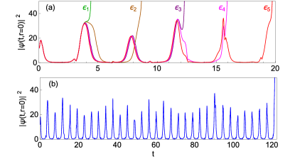
In $d=3$ without trapping potential, there is also a sharp separation between direct collapse and dispersion. With a harmonic potential, apart from having periodic stationary solutions PhysRevA.51.4704 ; PhysRevE.92.013201 , delayed collapses are possible. Figure 1 shows several examples. Each line of the plot is found by numerically integrating Eq. (1) with initial conditions (8). The different initial conditions have all the same width $\sigma$ but different values of the height $\epsilon$. We represent the value of $|\psi|^{2}$ at the origin. Collapse happens when this quantity diverges. For each initial condition, we can therefore compute the time of collapse $t_{c}$. There is an oscillating behavior which can be heuristically understood in terms of the linear problem (see the appendix), for which it can be immediately checked that $|\psi(r)|^{2}$ returns to itself with time period $\pi$. The same period is directly read from Eq. (4), since the last term is not present in the linear case. When the nonlinear term is present, the oscillation is only approximate and the “period” for which maxima appear in Fig. 1 is not exactly $\pi$. At each bounce inside the harmonic potential, the spatial profile of $|\psi|^{2}$ is modified and, eventually, this can result in a delayed collapse after several or many swings. This number of oscillations can be adjusted by fine-tuning the initial conditions. We call delayed collapses those which happen after one or more oscillations, like all the examples in the figure.

Figure 1: Examples of delayed collapses in $d=3$. We depict the value of $|\psi(t,r=0)|^{2}$ for $\sigma^{2}=2/5$ and varying $\epsilon$. In each case, the wavefunction promptly collapses after hitting the upper limit of the plot. In panel (a), ordered by growing $t_{c}$, we have $\epsilon_{1}=3.1286$ (green line), $\epsilon_{2}$=3.1285 (brown), $\epsilon_{3}$=3.1280 (purple), $\epsilon_{4}$=3.1277 (magenta) and $\epsilon_{5}$=3.1273 (red). Notice the approximate overlap for long ranges of $t$. In panel (b), $\epsilon_{6}=3.1270$ (blue line) results in collapse after many bounces. We remark that the time scale of both graphs is different.

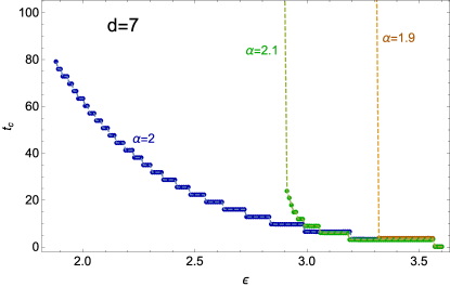
In figure 2, we plot the time of collapse, $t_{c}$, as a function of $\epsilon$ for fixed $\sigma^{2}=1/2$. Each red dot corresponds to a full simulation of Eq. (1) for which we find $t_{c}$ as in Fig. 1. Necessarily, the computation has to be stopped at some value of $t=t_{comp}$. If collapse has not been found by that time, it means that $t_{c}>t_{comp}$ or, possibly, there is no collapse in any finite time. In Fig. 2 we have taken $t_{comp}=140$ and the non-collapsing points are represented by the dotted line going up the top of the graph.

Figure 2: Time of collapse for a family of initial conditions with $\sigma^{2}=1/2$ in $d=3$. Prompt collapse occurs for $\epsilon>2.891$. The resolution of the peak at the transition $\epsilon\sim 2.889$ exhibits a chaotic structure (in the inset).

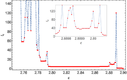
There are three distinct regions in parameter space. For large $\epsilon$ ($\epsilon>2.891$ in the case of Fig. 2), there is direct collapse and $t_{c}$ decreases with growing $\epsilon$. For small $\epsilon$ ($\epsilon<2.755$ in the case of Fig. 2), solutions stay regular for $t<t_{comp}$. There is a noteworthy intermediate transition region where some step structure is apparent (cf. $2.755<\epsilon<2.891$ in Fig. 2). Roughly speaking, each step corresponds to a number of bounces in the harmonic potential. At the boundary between steps, $t_{c}$ presents a bump. Our plot shows remarkable features in common with those found in different AdS setups (cf. Figs. 9 in buchel2013boson , 3 in cardoso2016collapsing , 16 in arias2016stability or 2 in deppe2015stability ). The chaotic character of the curve at the bumps has been recently established in Deppe:2016dcr . An analogous detailed analysis for this case would be of interest but extends way beyond the scope of this paper and is left for future work. The common feature of these examples seems to be the lack of fully resonant linearized perturbations around a standing wave Maliborski:2014rma .

Figure 3 depicts a map of the results obtained with different $\epsilon$ and $\sigma$, found by repeated simulations of Eq. (1) with different initial conditions (notice that the computations leading to Fig. 2 correspond to a vertical line at fixed $\sigma=0.707$ around the delayed collapse region). The transition line between prompt and delayed collapse can be defined with precision. On the other hand, regularity of evolution can only be stated within a given computational time, which we have fixed to $t_{comp}=100$ for Fig. 3. The delayed collapse window is certainly narrow in the two-parameter space of initial conditions.

Figure 3: Sectors for prompt and delayed collapse in $d=3$. The dashed line signals the transition from initial conditions where $d^{2}V/dt^{2}|_{t=0}$ changes from negative (above) to positive (below). All delayed collapses happen with $V\neq 0$.

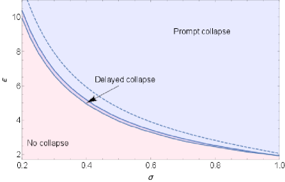
Tuning $\epsilon$ is equivalent to tuning the scattering length in the cold atom framework. Thus, Fig. 2 depicts the same observable as, e.g., Fig. 2 of donley2001dynamics . Our work is devoted to the theoretical analysis of Eq. (1) and we do not intend here to make a realistic description of experimental situations, where, typically, anisotropies and nonlinear losses should be taken into account. In any case, it is interesting to make order of magnitude estimates of the parameters. We take Fig. 2 of donley2001dynamics for reference. There, the harmonic trap is mildly anisotropic with $\nu_{radial}=17.5$Hz and $\nu_{axial}$=6.8Hz. Let us take a fiducial value of that order of magnitude $\nu=14$Hz. The initial condition is the ground state of the linear problem, namely $\sigma=\sqrt{2}$. In Fig. 3, it is shown that the delayed collapse window in parameter space closes around $\sigma=1$ and therefore the original atom cloud of donley2001dynamics is too wide to produce the behavior described here. Let us however compute the range of $\epsilon$ corresponding to the horizontal axis of Fig. 2 of donley2001dynamics . The relation between the physical and the adimensional quantities is provided in the appendix and we take $\bar{N}=6000$ for the number of atoms and $m=1.4\times 10^{-25}$kg (for ⁸⁵Rb). It is straightforward to show that $4<|a|/a_{0}<60$, where $a_{0}$ is the Bohr radius corresponds to $1<\epsilon<3.8$. The situation described in the present paper could be thus approached by taking an isotropic trap and starting with a narrower profile. Experimentally, smaller values of the initial $\sigma$ should be attainable by taking a tighter trap for $t<0$. At $t=0$, the trap can be ramped down while the value of $|a|$ is ramped up. Imagine a situation with $\sigma^{2}=1/2$ and the rest of parameters fixed as above. The $2.75<\epsilon<2.90$ window of our Fig. 2 becomes $3.8<|a|/a_{0}<4.3$ in physical terms, values that are well within reach with Feshbach resonance techniques.

As mentioned above, our interest in looking for delayed collapses in GPE was sparked by the similar problem in the gravitational context of a scalar field coupled to gravity and a negative cosmological constant. Now we can reverse the lore, and ask ourselves what we can learn from this nonlinear system in regard to the important question of the instability of AdS. In fact, one advantage of this simple equation is the fact that we can tweak separate features independently, like the property of full resonance or the character of the nonlinearity. These features are utterly mixed in the gravitational setup and are difficult to disentangle Cai:2015jbs .

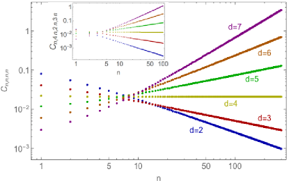
There is growing consensus that the weak turbulent instability of AdS, i.e., that initial data always collapse in the limit $\epsilon\to 0$, is not solely caused by a fully resonant spectrum. This being a necessary condition, needs to be supplemented with appropriate asymptotics for the coupling coefficients $C_{ijkl}$ (7) at large values of $i,j,k,l\to\infty$ in a resonant channel. This should catalyse efficient energy transfer to the high frequency modes. In the three-dimensional GPE, we have checked that $C_{in,jn,kn,ln}$ behaves with $n\to\infty$ as a power $n^{\gamma}$ with $\gamma=-0.5$. This is substantially lower a growth than the one observed in $AdS_{4}$ where $\gamma=1$ in this channel Craps:2015iia (in order to compare the resonant system in AdS with ours in Eq. (6), the modes $\alpha_{i}$ need to be rescaled to $\alpha_{i}/\sqrt{\omega_{i}}$. This shifts $\gamma=d\to d-2$).

A natural question is what minimal twist could we perform in order to enhance the asymptotics, and whether this would have the expected impact on the collapse at low values of the initial amplitude. One possibility is to include derivative terms, (derivative couplings appear in the effective equations for a scalar field coupled to gravity). In fact, a term of the form $|\partial_{r}\psi|^{2}\psi$ added to the GPE yields $\gamma\approx 0.5$. The numerical evolution of the system with this additional term becomes unstable and we have deferred its study.

Another artificial but efficient way to enhance $\gamma$ is to formally extend the GPE to higher dimensions. In figure 4, we depict the behavior of $C_{nnnn}$ for $n\leq 300$ and $d=2,\dots,7$. In the large $n$ limit the exponent $\gamma$ behaves with the dimension as (see the appendix)

$$\gamma=\frac{d}{2}-2,$$ (9)

a fact that presumably causes the different qualitative behavior between $d=2$ and $d=3$. This suggests that turbulence and collapse are favored at large $d$. This expectation is borne out by the results of figure 5, which shows a neat step structure for $t_{c}(\epsilon)$ when $d=7$, resembling $AdS_{4}$ Bizon:2011gg .

We also display the results with a slightly modified potential $V(r)=\frac{1}{2}r^{\alpha}$, where $\alpha=2$ corresponds to the harmonic case. Changing $\alpha$ modifies the eigenvalues of the linear problem, breaking full resonance. As shown in fig. 5 this has a dramatic impact on the time of collapse at low initial amplitudes.

Figure 4: Doubly logarithmic plot of $C_{nnnn}$ as a function of $n$ for different values of $d$. In the inset, we depict the $C_{n,4n,2n,3n}$, showing that they present a similar behavior.

Figure 5: Curve of $t_{c}$ vs. $\epsilon$ for $d=7$ with $\sigma^{2}=\frac{1}{2}$ and $V(r)=\frac{1}{2}r^{\alpha}$. Two non-resonant cases $\alpha=1.9$ and $\alpha=2.1$ present limiting values of $\epsilon$ below which no singularity is reached in computational time. The harmonic resonant case $\alpha=2$ (Eq. (1)) shows a regularly spaced set of steps extending to much lower values of $\epsilon$.

IV IV. Summary of results and connections to AdS gravity

Collapses in GPE/NLSE have been thoroughly studied but are still a fascinating topic. We have considered a harmonic trap in different number of dimensions. We have studied the long time evolution of the wave function for families of gaussian initial conditions depending on two parameters. For long time evolution we mean that many bounces are allowed to take place by evolving up to a time $t_{comp}\gg\pi$, which is much larger than that of an oscillation in the potential (we have seen that nonlinear oscillations do not have exactly a period $\pi$ but are associated to time spans of that order). In $d=3$, we have seen that there are initial conditions that lead to delayed collapses, where the divergence occurs after a number of oscillations, Fig. 1. On average, the time of collapse grows with the inverse of the norm of the initial wavefunction, but non-monotonically and with a strong sensitivity to the initial condition. This happens in a region of parameter space which separates direct collapse from absence of collapse, Figs. 2 and 3. In $d=7$, delayed collapses are also present, albeit of a different type. A neat step structure appears, cf. Fig. 5, which extends collapse to smaller values of $\epsilon$. This happens thanks to a fully resonant spectrum and efficient energy transfer between modes, associated to rapidly growing $C_{ijlm}$ couplings, Fig. 4.

For completeness, in Fig.6 we have plotted the behavior of the energy spectrum as a function of time for some of the modes. We do not include more modes for clarity of the plot. Besides the usual direct cascade that feeds the higher modes from the lowest ones, we also observe an inverse cascade. This is a consequence of the simultaneous conservation of two independent quantities, $N$ and $H$, and matches the similar behaviour observed in the resonant system obtained from averaging the AdS dynamics (see section III in Buchel:2014xwa ).

Figure 6: Temporal evolution of the spectrum $E_{n}=\mu_{n}|\alpha_{n}|^{2}$ for some low-lying modes until collapse. Panel (a) corresponds to an example with $d=3$. Panel (b) corresponds to an example with $d=7$. The changes in the spectrum mostly take place around the time when the wavefunction periodically peaks at the origin. This periodic energy transfer towards the ultraviolet underlies the stepwise patterns of collapse in figures 2 and 5.

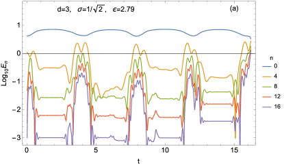
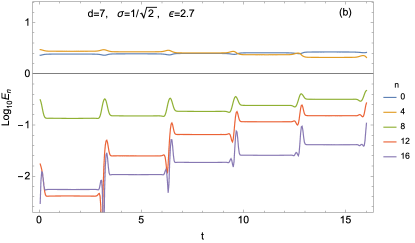
The transitions between steps in Fig. 6 happens at the time when the pulse comes close to the origin. A similar structure is seen in AdS and stems from the fact that the magnitude of the wave function increases by orders of magnitude, enhancing the non-linear effects at those instants of time. In $d=7$, this process is very much ordered and seems to end up inexorably in a collapse whereby a polinomially decaying spectrum is achieved. In $d=3$ the ordered structure is less apparent and the process becomes a statistical wave turbulence effect.

One may wonder is how generic the described behavior is. One intriguing answer is given by comparing to a scalar field in AdS gravity which shows remarkable similarities. Indeed, the two-fold structure with (partially) chaotic and ordered delayed collapses has been described in that context, see the references provided in the previous section.

In summary, we have found an interesting structure in the space of evolutions leading to collapse, within the simple setup of Eq. (1). There are neat similarities with those encountered in the context of gravitational dynamics in AdS. Since the inherent physics and the evolution equations are rather different in both cases, a natural question is what underlying mechanisms are at work. Both cases have an attractive nonlinearity that can bunch together the energy and produce a collapse that alters the otherwise smooth evolution. The harmonic potential and the AdS boundary act as boxes that impede the escape of the perturbation to infinity and cause the bounces. Moreover, they both provide a fully resonant spectrum for the linear modes. In both cases, there is an effective equation (6) and the resonant channels and conserved quantities coincide. These observations might be useful to identify other frameworks in which similar phenomena take place. Nevertheless, solid conclusions can only be derived from full-fledged numerical analysis.

Turbulence and energy cascades constitute an active area of research in the context of GPE, see e.g. shukla2013turbulence carles2010energy ; turbu1 ; turbu2 , and especially Tsatsos2016 for a recent review with references. Our setup differs from these works in several aspects, including the presence of the harmonic term and the assumed radially symmetric evolution. It could be interesting to explore whether insights from the quoted studies have implications in the present context.

V V. Outlook

The GPE/NLSE is an ubiquitous formalism in nonlinear waves, and this fact can pave the way for tabletop experiments with qualitative analogies to AdS gravity. The experimental control reached in BECs might provide an ideal framework to realize the delayed collapse phenomenology. Our formalism is not a complete description of any such system since, for instance, it does not include anisotropies or losses by three-body recombinations. However, our results suggest that it might be worth revisiting, theoretically and/or experimentally, the transition from a stable BEC with attractive nonlinearity to a Bosenova collapse (cf. Fig. 2 of donley2001dynamics ). Depending on the width of the initial wavefunction, $t_{c}$ can decrease with the strength of the interaction $|a|$, a counterintuitive behavior. Moreover, there are narrow regions of parameter space where $t_{c}$ changes chaotically. Whether these properties stemming from Eq. (1) can be consequential in a realistic setup is a challenging question for the future.

Our model can also be used as a mathematical tool to provide new insights to the problem of AdS instability. The GPE evolution equation is much simpler than those of AdS gravity but, as we have discussed, its study might be instrumental in understanding which peculiarities of general relativity are essential for the delayed collapse behavior and which are shared by other kinds of nonlinear systems. Moreover, it provides turning knobs that can be used to investigate which qualitative features (e.g full resonance, efficient turbulent cascades, etc.) underlay the remarkable nonlinear dynamics that has been discovered in the AdS context in recent years. For instance, the behavior of the $C_{ijkl}$ coefficients (7) can be tuned by considering larger dimensions, nontrivial spatial profiles for the nonlinear coupling or other generalizations of Eq. (1). On the other hand, full resonance can be broken by slightly modifying the potential. We hope that a detailed scrutiny of these issues will shed new light on this fascinating nonlinear dynamics.

Appendix

In this appendix we lay out some technicalities related to the main text. We write down some useful well-known equations concerning the dimensionful Gross-Pitaevskii equation (GPE) and the radially symmetric eigenmodes of a harmonic potential in $d\geq 2$ dimensions. Then, we specify some details regarding the employed numerical methods and cross-checks. Finally, we explain how the asymptotic form of the $C_{ijkl}$ coefficients can be derived from the integrals.

.1 The $d=3$ dimensionful GPE

The Gross-Pitaevskii mean-field description of a dilute Bose-Einstein condensate of bosons of mass $m$ in an isotropic harmonic potential of frequency $\omega$ is:

$$i\hbar\partial_{\tilde{t}}\tilde{\psi}=-\frac{\hbar^{2}}{2m}\tilde{\nabla}^{2}\tilde{\psi}+\frac{m\omega^{2}}{2}\tilde{r}^{2}\tilde{\psi}+\frac{4\pi\hbar^{2}a}{m}|\tilde{\psi}|^{2}\tilde{\psi}$$ (10)

where $\tilde{\nabla}^{2}$ is the $3-$dimensional Laplacian, $a$ is the s-wave scattering length which can be positive (repulsive interaction) or negative (attractive interaction) and $\tilde{N}=\int|\tilde{\psi}|^{2}d^{3}\tilde{\bf r}$ corresponds to the number of bosons in the sample. Eq. (1) is recovered by appropriately rescaling $\tilde{t}$, $\tilde{r}$ and $\tilde{\psi}$. The relation between normalizations is $\tilde{N}=\frac{1}{4\pi|a|}\sqrt{\frac{\hbar}{m\omega}}N$.

.2 Eigenfunctions of the harmonic oscillator

The angle-independent eigenfunctions of the linear quantum harmonic oscillator with $d\geq 2$ are

$$\psi_{n}=e^{-i\mu_{n}^{(d)}t}f_{n}^{(d)}(r)\,$$ (11)

with a fully resonant spectrum $\mu^{(d)}_{n}=2n+d/2$ and

$$f_{n}^{(d)}(r)=\sqrt{\frac{n!\Gamma(\frac{d}{2})}{\pi^{d/2}\Gamma(\frac{d}{2}+n)}}\ L_{n}^{(d-2)/2}(r^{2})e^{-r^{2}/2}\,.$$ (12)

The $L_{n}^{(d-2)/2}$ are generalized Laguerre polynomials, $\Gamma$ represents Euler’s gamma function and the multiplicative constant is chosen to satisfy the orthonormality condition $\int f_{n}^{(d)}f_{m}^{(d)}d^{d}{\bf r}=\delta_{nm}.$

.3 Numerical details and quality checks

In the region of delayed collapses, small changes in initial conditions can lead to rather different results. Thus, a method for fast, stable and precise computation is needed and we briefly describe here the one we have used. Our integration algorithm relies on an explicit finite difference scheme consistent with fourth order accuracy and convergence. Spatial derivatives are discretized with standard stencils, and time evolution uses a fourth order Runge-Kutta. The Courant factor, $c$, depends on the discretization density since the equation is parabolic. Stability enforces this number to be quite small. For $2^{w}$ points in the spatial grid, we have used $c=0.004\times 2^{12-w}$ with $w=12,...,17$.

At the origin, we ensure regularity by enforcing $\partial_{r}\psi(t,r=0)=0$. The harmonic potential confines the wavefunction and therefore $\psi$ decays exponentially with $r$. We have checked that choosing $r_{max}=50$ keeps $\psi(r_{max})\sim 10^{-15}$ so that setting its value to zero, and truncating $r$ to a finite interval $0<r<r_{max}$, does not affect the simulation. We have also performed computations using a truly compact coordinate $r=z/(z_{max}-z)$ and found consistent results.

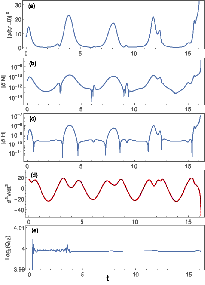
We have used the conservation of the norm (2), the hamiltonian (3), and the variance identity (4), as quality tests to monitor the computation. For initial conditions of the form (8), they take the values

$$N = \left(\frac{\pi}{2}\right)^{\frac{d}{2}}\epsilon^{2}\sigma^{d}\,,$$

$$H = \frac{d}{2}\left(\frac{\pi}{2}\right)^{\frac{d}{2}}\epsilon^{2}\sigma^{d}\left(\frac{1}{\sigma^{2}}+\frac{\sigma^{2}}{4}-\frac{\epsilon^{2}}{2^{\frac{d}{2}}d}\right)\,.$$ (13)

The value of the second derivative of the variance at $t=0$ is:

$$\left.\frac{d^{2}V}{dt^{2}}\right|_{t=0}=2d\left(\frac{\pi}{2}\right)^{\frac{d}{2}}\epsilon^{2}\sigma^{d}\left(\frac{1}{\sigma^{2}}-\frac{\sigma^{2}}{4}-\frac{\epsilon^{2}}{2^{\frac{d}{2}+1}}\right)\,.$$ (14)

We define the relative deviations $\delta N=\frac{N_{num}-N}{N}$, $\delta H=\frac{H_{num}-H}{H}$ where $N_{num}$, $H_{num}$ are the values obtained from numerical integration and $N$, $H$ are the values given in (13). To keep them satisfied at relative orders $\delta H,\delta N<10^{-6}$ we have implemented global (in space) refinement. This is seen to be required when the profile becomes extremely sharp at the origin, and needs more resolution to keep numerical control. Fig. 7 depicts a check for one of the simulations yielding a delayed collapse.

Figure 7: A simulation with $d=3$, $\epsilon=2.79$ , $w=14$, $\sigma^{2}=1/2$. Panel (a) represents $|\psi|^{2}$ at the origin. Panels (b) and (c) depict the relative deviations for the norm and hamiltonian, respectively. Panel (d) compares the second derivative of the variance from the numerical computation to that from the right-hand side of Eq. (4) computed at each step. Finally, panel (e) shows the convergence level along the whole simulation. On a grid of $2^{w}$ points, $Q_{w}=||\psi_{w+1}-\psi_{w}||/||\psi_{w+2}-\psi_{w+1}||$ where $||\cdot||$ stands for a $L^{2}$ norm. The plot shows convergence at fourth order with high accuracy. The tests show that the numerical method is reliable until times very near collapse.

We have implemented our codes for CPU computation and, in order to speed up the simulation, we also adapted them for GPGPU. The computation times that we achieve are approximately one order of magnitude lower in the latter case.

.4 Asymptotic values of the $C_{ijkl}$

We now obtain the asymptotically large $n$ behaviour of $C_{n\left(ijkl\right)}$. The form of the coefficients is given by the integral in (7) for the eigenfunctions of Eq. (12). We follow the procedure of Evnin:2016mjx . Consider the identity Digital

$$L_{n}^{(\alpha)}(\nu x)\approx\frac{e^{\frac{1}{2}\nu x}}{2^{\alpha}x^{\frac{1}{2}\alpha+\frac{1}{4}}}\left(\xi^{1/2}J_{\alpha}(\nu\xi)\right)$$ (15)

valid in the limit $n\to\infty$, $x\ll 1$. $J_{\alpha}(x)$ are Bessel functions of the first kind and $\alpha=\frac{d}{2}-1$, $\nu=2\mu_{n}^{(d)}$, $\xi\approx\sqrt{x}$. Taking $r^{2}=\nu x$, we get an expression for the eigenfunctions. Notice that the limit $x\ll 1$ is justified because $x=r^{2}/n$ with $n\rightarrow\infty$.

Now the Bessel functions are $J_{\alpha}(\nu^{1/2}r)$ and performing a change of variables in the integral (7), we can remove the dependence in $n$ from the argument. Using the asymptotic value for the normalization constants (cf. the prefactors in (12)) $N_{n}\sim n^{-\alpha/2}$, we obtain $C_{n\left(ijkl\right)}\sim n^{\frac{d}{2}-2}\int dzK(z)$ where $K(z)$ does not depend on $n$. Thus, we get equation (9).

We have checked that this expression is in agreement with the values of $C_{nnnn}$ and $C_{n,4n,2n,3n}$ found by numerical integration for $d=2,\dots,7$, see figure 4.