L-space knots
Abstract. We characterize the knots in the three-sphere and lens spaces that admit non-trivial L-space surgeries. As a corollary, 1-bridge braids in these manifolds admit non-trivial L-space surgeries. We also recover a characterization of the Berge manifold amongst 1-bridge braid exteriors.
1. Introduction.
An L-space is a rational homology sphere with the “simplest” Heegaard Floer invariant: is a free abelian group of rank . Examples abound and include lens spaces and, more generally, connected sums of manifolds with elliptic geometry [OS05]. One of the most prominent problems in relating Heegaard Floer homology to low-dimensional topology is to give a topological characterization of L-spaces. Work by many researchers has synthesized a bold and intriguing proposal that seeks to do so in terms of taut foliations and orderability of the fundamental group [Juh15, Conjecture 5].
A prominent source of L-spaces arises from surgeries along knots. Suppose that is a knot in a closed three-manifold . If admits a non-trivial surgery to an L-space, then is an L-space knot. Examples include torus knots and, more generally, Berge knots in [Ber]; two more constructions especially pertinent to our work appear in [HLV14, Vaf15]. If an L-space knot admits more than one L-space surgery – for instance, if itself is an L-space – then it admits an interval of L-space surgery slopes, so it generates abundant examples of L-spaces [RR15]. With the lack of a compelling guiding conjecture as to which knots are L-space knots, and as a probe of the L-space conjecture mentioned above, it is valuable to catalog which knots in various special families are L-space knots. This is the theme of the present work.
The manifolds in which we operate are the rational homology spheres that admit a genus one Heegaard splitting, namely the three-sphere and lens spaces. The knots we consider are the knots in these spaces: these are the knots that can be isotoped to meet each Heegaard solid torus in a properly embedded, boundary-parallel arc. Our main result, Theorem 1.2 below, characterizes L-space knots in simple, diagrammatic terms.
A diagram is a doubly-pointed Heegaard diagram , where is a genus one Heegaard diagram of a 3-manifold . The knots in are precisely those that admit a doubly-pointed Heegaard diagram [GMM05, Hed11, Ras05]. A diagram is reduced if every bigon contains a basepoint. We can transform a given diagram of into a reduced diagram of by isotoping the curves into minimal position in the complement of the basepoints: we accomplish this by successively isotoping away bigons in the complement of the basepoints and the curves in . Our characterization of L-space knots in and lens spaces is expressed in terms of the following property of diagrams:
Definition 1.1.
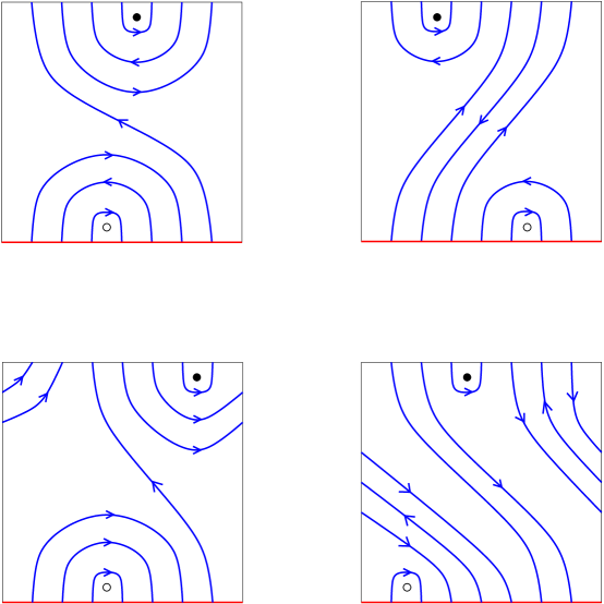
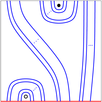
A reduced diagram is coherent if there exist orientations on and that induce coherent orientations on the boundary of every embedded bigon . Its sign, positive or negative, is the sign of , with these curves coherently oriented.
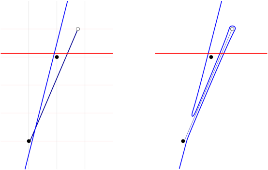
Coherence is easy to spot in a diagram: see Figures 1 and 2 and the second paragraph of Subsection 2.3.
We may now state the main result of the paper:
Theorem 1.2.
A reduced diagram presents an L-space knot if and only if it is coherent. The knot is a positive or negative L-space knot according to the sign of the coherent diagram.
The sign of an L-space knot is the sign of an L-space surgery slope along it, which we review in Subsection 2.1. Note that a given knot may admit non-homeomorphic coherent diagrams. However, Theorem 1.2 implies that its reduced diagrams are either all incoherent or else all coherent and of the same sign. Again, see Figure 1.
We apply Theorem 1.2 to show that a broad family of knots are L-space knots. We recall the following construction, first studied by Berge [Ber91] and Gabai [Gab90], and state a natural generalization of it.
Definition 1.3.
A knot in the solid torus is a 1-bridge braid if it is isotopic to a union of two arcs such that
-
•
is braided, i.e., transverse to each meridian , and
-
•
is a bridge, i.e., properly embedded in some meridional disk .
It is positive if is a positive braid in the usual sense. A knot in a closed three-manifold with a genus one Heegaard splitting is a 1-bridge braid if it is isotopic to a 1-bridge braid supported within one of the Heegaard solid tori.
J. and S. Rasmussen conjectured that a positive 1-bridge braid in is a positive L-space knot at the end of [RR15]. We prove a generalization of their conjecture in Theorem 3.2. Without the sign refinement, the result reads:
Theorem 1.4.
1-bridge braids in and lens spaces are L-space knots.
Krcatovich has found many examples of L-space knots in that are not 1-bridge braids by a computer search [Krc]. A small representative is the knot in the notation of [Ras05]. He showed that it is an L-space knot by an application of Theorem 1.2, and that its Alexander polynomial distinguishes it from 1-bridge braids by comparing with a list tabulated by J. Rasmussen.
We collect the necessary background on Heegaard Floer homology and prove Theorem 1.2 in Section 2. We prove Theorem 1.4 and its sign-refined version, Theorem 3.2, in Section 3. We also use Theorem 3.2 to characterize the Berge manifold in Proposition 3.4.
We leave open two natural problems: the isotopy classification of L-space knots, and the determination of whether surgeries along these knots conform to [Juh15, Conjecture 5].
Acknowledgments.
We thank Matt Hedden, Jen Hom, David Krcatovich, Adam Levine, Clayton McDonald, Yi Ni, and Alex Zupan for helpful conversations. We thank the referee for a very thorough and thoughtful review. Sam Lewallen would like to thank Zoltán Szabó for suggesting he study L-space knots, and both Zoltán and Liam Watson for their interest and encouragement. JEG was supported by NSF CAREER Award DMS-1455132 and an Alfred P. Sloan Foundation Research Fellowship. SL was supported by an NSF Graduate Research Fellowship.
2. Proof of the characterization.
We assume familiarity with (knot) Floer homology and review the essential input for our work in Subsections 2.1 and 2.2. In particular, we follow the treatment of [RR15, §2.2], with slight differences in notation. We prove Theorem 1.2 in Section 2.3.
2.1. Knot Floer homology and L-space knots.
Let denote a (doubly pointed) knot in a rational homology sphere . Let denote an open tubular neighborhood of , the knot exterior, and a meridian of . Let denote the set of structures on and the set of relative structures on . They are torsors over the groups and , respectively. Let denote the set of orbits in under the action by . It forms a torsor over , and there exists a pair of torsor isomorphisms .
We work with the hat-version of knot Floer homology with coefficients, graded by :
There exists a further pair of gradings
on each summand, the Alexander and Maslov gradings. An element is homogeneous if it is homogeneous with respect to both gradings. The group comes equipped with differentials , that preserve the -grading, respectively lower and by one, and respectively raise and lower . They are invariants of , and their homology calculates and , respectively. The manifold is an L-space if for all .
Definition 2.1.
For a knot in an L-space and , the group is a positive chain if it admits a homogeneous basis such that, for all ,
The group consists of positive chains if is a positive chain for all .
For example, a positive chain with generators takes the form shown here:
Each arrow represents a component of the differential and is an isomorphism between the groups it connects. Similarly, a negative chain is the dual complex to a positive chain with respect to the defining basis. Reversing the arrows above gives an example of a negative chain.
Note that the requirement that the positive chain basis elements are homogeneous does not appear in [RR15, Definition 3.1]. For example, we could alter the positive chain basis displayed above to an inhomogeneous one by replacing by . However, homogeneity is an intended property of a positive chain basis in the literature. Moreover, an inhomogeneous positive chain basis gives rise to a homogeneous one by replacing each basis element by its homogeneous part of highest bigrading. Therefore, our definition is no more restrictive, and its precision is more convenient when we invoke it in the proofs of Lemmas 2.3 and 2.4.
Let denote the rational longitude of , the unique slope that is rationally null-homologous in . Note that , since is a rational homology sphere. Another slope is positive or negative according to the sign of , for any orientations on these curves. The knot is a positive or a negative L-space knot if it has an L-space surgery slope of that sign. The following theorem characterizes positive L-space knots in L-spaces in terms of their knot Floer homology. Ozsváth and Szabó originally proved it for the case of knots in [OS05, Theorem 1.2]. Boileau, Boyer, Cebanu, and Walsh promoted a significant component of their result to knots in rational homology spheres [BBCW12]. Building on it, J. and S. Rasmussen established the definitive form of the result that we record here: see [RR15, Lemmas 3.2, 3.3, 3.5], including the proofs of these results.
Theorem 2.2.
A knot in an L-space is a positive L-space knot if and only if consists of positive chains. ∎
Similarly, is a negative L-space knot if and only if consists of negative chains. The reason amounts to the behavior of Dehn surgery and knot Floer homology under mirroring.
2.2. Calculating the invariants from a Heegaard diagram.
The invariants can be calculated from any doubly-pointed Heegaard diagram of after making some additional analytic choices. Here, as usual, denotes a closed, oriented surface of some genus ; and are -tuples of homologically linearly independent, disjoint, simple closed curves in ; and the two basepoints and lie in the complement of the and curves on . The curve collections induce tori in the -fold symmetric product . The underlying group of the Floer chain complex is freely generated by . The elements of fall into equivalence classes in 1-1 correspondence with : two elements lie in the same equivalence class iff the set of homotopy classes of Whitney disks from to is non-empty. Write for the equivalence class corresponding to and for the subgroup of generated by the elements in . Each Whitney disk has a pair of multiplicities , and a Maslov index . The Alexander and Maslov gradings on are characterized up to an overall shift by the relations
for all and . There exist endomorphisms of defined on generators by the same general prescription:
Here ranges over ; ranges over the elements of with Maslov index and a constraint on the multiplicities , ; and is the count of pseudo-holomorphic representatives of . The specific constraints on the multiplicities are for ; for ; and for . The maps are all differentials. The differential lowers by one and is filtered with respect to . The differential lowers by one and is filtered with respect to . The differential is the -filtration-preserving component of each. The groups , , and are the homology groups of with respect to , , and , respectively, and the Alexander and Maslov gradings on descend to the respective gradings on . The maps and induce the differentials and on , respectively.
The Alexander and Maslov gradings enable us to constrain the existence of pseudo-holomorphic disks for L-space knots.
Lemma 2.3.
Suppose that is a doubly-pointed Heegaard diagram for , vanishes on , and is a positive chain with basis . If there exist generators and a disk with and , then and for some . Furthermore, if and if .
Proof.
Definition 2.1 and the paragraph preceding it show that the positive chain basis satisfies
and
for some positive integers , . In particular, the Maslov and Alexander gradings of the both decrease with the index . The generators are homogeneous with respect to both gradings, as are the positive chain basis elements, so it follows that and for some , , and choices of sign.
The assumption that implies that , and at least one inequality is strict, since . Thus,
| (1) |
In the case of equality , then , and either , which gives the desired conclusion, or else , which we must rule out. In this case, and . Since is a rational homology sphere, it follows that is the unique disk with , so the coefficient on in is . However, this implies that , which violates the form of the positive chain.
Otherwise, , so . We have
| (2) |
Each term in the second sum is odd, and their total sum is odd, so it contains an odd number of terms. The terms of the first sum alternately take the form and , while the terms of the second sum alternately take the form and . Let denote the sum of the values that appear and the sum of the that appear. All of values are positive, so , and only if is even and , and only if is odd and . The first sum in (2) equals , while the second sum equals or , according to whether is even or odd. Comparing with the second sum in (1) gives or , according to whether is even or odd. Comparing with the first sum in (1) then gives or , according to whether is even or odd. If is even, then gives and , which gives the desired conclusion. If is odd, then again gives and . However, in this case it follows as before that appears with coefficient in , which once again violates the form of the positive chain. ∎
2.3. (1,1) knots.
Now assume that is a -diagram, so has genus one. In this case, the differentials on admit an explicit description that requires no analytic input, owing to the Riemann mapping theorem and the correspondence between holomorphic disks in the Riemann surface and its universal cover . Specifically, the conditions that and imply that for any choice of analytic data. Furthermore, these conditions are met if and only if the image of lifts under the universal covering map to a bigon cobounded by lifts of and . See [GMM05] and [OS04, pp.89-96] for more details.
Assuming now that is reduced, we have and . We proceed to analyze the differentials and . Without loss of generality, we henceforth fix , , a horizontal line , and . After a further homeomorphism, we may assume that takes the form shown in Figure 2. Observe that the embedded bigons in are the obvious ones cobounded by the with the “rainbow” arcs of above and below . Coherence is the condition that when the curve is oriented, all of the rainbow arcs around a fixed basepoint orient the same way. This makes it easy to check coherence from a diagram in standard form.
Let denote the upper and lower half-planes bounded by . Choose a lift to of any point in . There exists a unique lift that passes through it. The points of are in 1-1 correspondence with under , and there are an odd number of them, since with appropriate orientations on the curves. The curve meets each half-plane in one closed ray and compact arcs. These compact arcs cobound positive bigons and negative bigons with for . A positive bigon attains a local maximum, and its image under is the top of one of the rainbow arcs above . Consequently, it contains a lift of the bigon in cobounded by that rainbow arc with . Thus, , and similarly , for all . Lastly, the positive bigons go from their left-most corner to their right-most corner, and vice versa for the negative bigons.
Lemma 2.4.
If is a reduced diagram of and is a positive chain, then
-
(1)
and for all ;
-
(2)
the positive bigons are exactly the ones that contribute to , the negative bigons are exactly the ones that contribute to , and there are no other bigons; and
-
(3)
if and are oriented so that , then and induce coherent orientations on the boundaries of all of the bigons they cobound.
Proof.
∎
Drawing on the proof of Lemma 2.4, we make a definition and prove a converse.
Definition 2.5.
A curve is graphic if its intersection points with occur in the same or opposite orders along and . It is positive if they occur in opposite orders and negative if they occur in the same order.
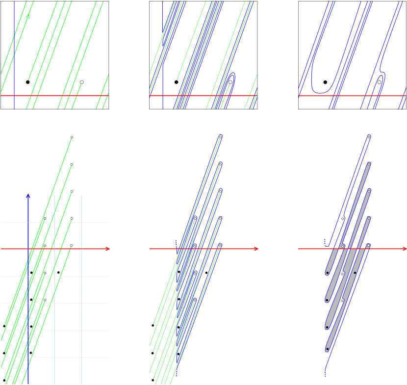
The bottom right picture in Figure 3 displays a positive graphic curve. The reason for the terminology is that a curve is graphic iff there exists a homeomorphism of taking to the pair consisting of the -axis and the graph of an odd degree polynomial with all roots real and distinct. Its sign, positive or negative, is minus the sign of the leading coefficient of the polynomial.
Proposition 2.6.
If is a reduced diagram of , then is a positive or a negative chain if and only if is positive or negative graphic, respectively.
Proof.
If is a positive chain, then Lemma 2.4 parts (2) and (3) show that is positive graphic. Conversely, suppose that is positive graphic. Label the points of intersection in by in the order they occur along . The only bigons cobounded by and are the positive and negative bigons. This latter fact can be verified using the equivalent definition of a graphic curve mentioned after Definition 2.5. Therefore,
for all and some . A value or is 0 iff the corresponding bigon contains both and basepoints. Since
it follows that for all , and is a positive chain. The corresponding statements for a negative chain and negative coherent diagram follow as well. ∎
Proof of Theorem 1.2.
Let denote a reduced -diagram of .
Suppose first that is a positive L-space knot. Orient and so that , and suppose that is an embedded bigon in . We must show that and coherently orient . Suppose that the corners of belong to , and let denote the lift of to with corners in . We have . Since is a positive L-space knot, Theorem 2.2 implies that is a positive chain, and by Lemma 2.4(3), the orientations on and coherently orient the boundaries of all of the bigons they cobound. In particular, they coherently orient , so and coherently orient . Therefore, is positive coherent.
Conversely, suppose that is positive coherent. Orient and so that and orients from left to right. Fix and select any . It is the endpoint of a closed ray of oriented out of it. If this ray meets in another point, then let denote the first such point. The arc of from to cobounds a bigon with . If lies to the left of , then is incoherently oriented by and . The arc of has an extremal (highest or lowest) point which lifts the extremal point of a rainbow arc. Projecting to by , it follows that this rainbow arc cobounds an embedded bigon with that is incoherently oriented by and , a contradiction. Therefore, lies to the right of . It follows by induction that the points of occur in the opposite orders along and with respect to these curves’ orientations. It follows that is graphic, and since , it is positive graphic. By Proposition 2.6, is a positive chain. Therefore, consists of positive chains, and is a positive L-space knot by Theorem 2.2.
The corresponding statements for negative coherent diagrams and negative L-space knots follow by a similar argument. ∎
3. 1-bridge braids.
This section consists of two parts. The first is devoted to the proof of Theorem 1.4 and its sign-refined version, Theorem 3.2. The second is a vignette on how Theorem 3.2 pertains to solid torus fillings on 1-bridge braid exteriors. Specifically, we give a novel argument in Proposition 3.4 to characterize the Berge manifold amongst 1-bridge braid exteriors.
3.1. 1-bridge braids are L-space knots
We prepare by describing a reduced -diagram of a 1-bridge braid in a rational homology sphere.
Let denote a 1-bridge braid. Identify with the flat torus in such a way that meridians lift to horizontal lines and longitudes lift to vertical lines under . Isotope rel endpoints into a geodesic on , so that consists of parallel line segments in of some common slope . Orient and write so that in each lift of to , the lift of lies below that of .
Form a genus one rational homology sphere by gluing a solid torus to along their boundaries, and let denote the image of in . Let denote a meridian of and let denote the curve to which the meridian of attaches, which we take to be a geodesic. In meridian-longitude coordinates, has some slope , and is homeomorphic to if and otherwise. Assume that and are disjoint from . Isotope by a finger-move along into a curve disjoint from . Observe that is a doubly-pointed Heegaard diagram for . Put it into reduced form by further isotoping so as to eliminate all bigons that do not contain basepoints, one by one, resulting in a curve . Let denote the resulting reduced diagram of . Figure 3 exhibits this procedure for the inclusion of the 1-bridge braid into , the pretzel knot . The notation derives from the braid presentation of 1-bridge braids; see [Ber91, Gab90, Wu04]. The –bridge braid denotes the closure of the braid word in , where the are the generators of the braid group . Note that and differ by a full twist, so there is a diffeomorphism of the solid torus that carries one to the other. Therefore, we may assume that .
A pair of distinct slopes determines an interval oriented from to in the counterclockwise sense; thus, and .
Proposition 3.1.
The diagram is coherent. Furthermore, it is positive if and negative if .
Note that Proposition 3.1 does not characterize the sign of the coherence in terms of . Theorem 3.2 does so in terms of the slope interval, and its proof relies on Proposition 3.1.
Proof.
Choose lifts of and to . They meet in a single point of intersection . Consider the lifts of that meet both and and in that order relative to their lifted orientations. Observe that these lifts meet the same component of . Label the points of intersection between these lifts and by in the order that they appear along this component, moving away from . The isotopy from to lifts to one from to . Nearby each is a pair of intersection points between and . The points occur in that order along both and . Thus, is graphic. The isotopy from to lifts to one from to . Each elimination of a bigon eliminates a pair of intersection points that are consecutive along both and . Therefore, the intersection points between and are a subset of those between and , and they occur in the same order along and . It follows that is graphic, as well. Furthermore, is positive graphic if the -coordinates of decrease with index and negative graphic if they increase with index. This is the case if belongs to or in , respectively. In particular, it is independent of the choice of lift of . Thus, all lifts of are -graphic for the same choice of sign . It follows that is coherent, and the sign-refined statement follows as well. ∎
We proceed to sharpen the statement of Theorem 1.4. To do so, we introduce the notion of a strict 1-bridge braid and its basic invariants: the winding number and slope interval. Choose the lift of with one endpoint at . Its other endpoint takes the form . We have by our convention on the basepoints, and is not a proper divisor of . Moreover, is an invariant of the isotopy type of , since . This is the winding number .
Consider the sweep-out of line segments with one endpoint at and the other endpoint varying along line . There exists a maximal slope interval containing and so that the sweep-out of line segments through slopes in contains no lattice point in its interior. If , then , and otherwise with . The sweep-out descends to an isotopy through 1-bridge braids with slopes in the interior of . If a line segment of slope has endpoint , then write , where . Let denote the meridian of the torus knot and the surface framing, oriented so that . If , then is isotopic to the torus knot , and if , then is isotopic to the -cable of , where the sign is positive or negative if the slope of the line segment is or , respectively. We call such a cable an exceptional cable of a torus knot. Otherwise, if no line segment has endpoint , then we call a strict 1-bridge braid (and justify the terminology in Corollary 3.3). In this case, there exists a unique so that , and and are consecutive terms in the Farey sequence of fractions from to whose denominators are bounded by when expressed in lowest terms.
For the following result, assume are coprime integers, and let denote . A simple knot in is a knot whose defining arcs are contained in meridian disks in the respective Heegaard solid tori, where the disks’ boundaries meet in transverse points of intersection. We permit the degenerate case that the the cable arc is a simple closed curve and the bridge is a point, in which case the simple knot is an unknot. Equivalently, a simple knot is a knot admitting a diagram in which all points of intersection between and have the same sign. Note that every simple knot is a 1-bridge braid: to see this, push one of the defining arcs onto the Heegaard torus.
Theorem 3.2.
The inclusion of a strict 1-bridge braid into is
-
(1)
a positive L-space knot iff ;
-
(2)
a negative L-space knot iff ; and
-
(3)
a simple knot iff .
For example, the inclusion of into is a simple knot iff .
Proof of Theorem 3.2.
For the forward directions, suppose first that . Write in lowest terms, . As before, let denote the lift of with one endpoint at and the other at . Note that . Let denote a horizontal line that separates from , and let denote a line of slope that separates from . Then , , and intersect in pairs, and since , they cobound a triangle containing in its interior. See Figure 5(a).
Follow the procedure for producing a coherent diagram for using the curves . The isotopy from to captures in a negative bigon and in a positive bigon in . See Figure 5(b). These points remain in bigons of the respective types following the isotopy from to . It follows that is a positive chain of rank greater than one for the structure corresponding to the pair of lifts . Thus, is not a negative L-space knot, which gives the forward direction of (2). The forward direction of (1) follows the same line of reasoning.
Since a simple knot is both a positive and a negative L-space knot, the forward direction of (3) follows. Finally, taking a 1-bridge presentation of in which has slope results in a diagram of a simple knot, and the reverse direction of (3) follows. ∎
The following result recovers the isotopy classification of 1-bridge braids from Theorem 3.2. Compare [Gab90, Proposition 2.3], which does so in terms of braid parameters.
Corollary 3.3.
If is a strict 1-bridge braid, then the slope interval is an invariant of the isotopy type of . Its isotopy type is determined by its slope interval and winding number, and is not isotopic to a torus knot or an exceptional cable thereof.
Proof.
The slope interval is characterized by Theorem 3.2 as the set of surgery slopes for which includes as a simple knot, so it is an isotopy invariant. It and the winding number together determine a sweep-out of arcs which in turn specify the isotopy type of . If is a strict 1-bridge braid, then it does not include as a simple knot in any lens space of order or less. However, every torus knot and exceptional cable thereof includes as an unknot in the lens space obtained by -filling on the outer torus. ∎
3.2. Solid torus fillings.
Gabai proved that a knot in the solid torus with a non-trivial solid torus surgery is a 1-bridge braid in [Gab90], and Berge classified them in [Ber91]. Berge found that, up to mirroring, is the unique strict 1-bridge braid that admits more than one such surgery. Its exterior is known as the Berge manifold. Menasco and Zhang studied 1-bridge braids whose exteriors admit a solid torus filling on the outer torus in [MZ01], and Wu classified them in [Wu04].
We indicate a line of approach towards Wu’s result using Theorem 3.2. Suppose that is a 1-bridge braid in and -filling on its outer torus is a solid torus; equivalently, the inclusion of into is a knot with solid torus exterior. A knot in has a solid torus exterior if and only if it is simple and homologous to the oriented core of a Heegaard solid torus. Since equals times a generator of , the uniqueness of genus one Heegaard splittings of implies that either
| (3) |
the possibilities correspond to the two Heegaard solid tori and the two orientations. Therefore, Theorem 3.2 reduces the problem Wu solved to one about lattice points. However, it appears to require considerable effort to extract Wu’s result from it. Nevertheless, we can quickly derive the following characterization of the Berge manifold:
Proposition 3.4.
Up to mirroring, the knot is the unique strict 1-bridge braid whose exterior admits three distinct solid torus fillings on the outer torus.
Wu points out that this result follows from the work of Berge and Gabai, which is an amusing exercise [Wu04, §4(1)]. By contrast, we deduce Proposition 3.4 from Theorem 3.2 and the uniqueness of genus one Heegaard splittings of lens spaces.
Given linearly independent , let denote the triangle with vertices , , . It is empty if it contains no lattice points besides its vertices, i.e. is a basis of .
Proof.
Suppose that is a strict 1-bridge braid with winding number and slope interval , . Let denote the exterior of . Suppose that -Dehn filling on the outer torus of is a solid torus. Thus, , and one of the congruences in (3) holds.
If (3)(b) holds, then there must exist so that is empty. If , then this triangle contains if and if . Therefore, we must have . Furthermore, if and if .
If instead , then it follows that (3)(a) holds, and we obtain . Furthermore, is in the cone bounded by the rays from through and . Since , it follows that . Moreover, is the mediant of and , meaning that and .
Hence, if has three distinct solid torus fillings, then they have slopes , , and (in conformity with the cyclic surgery theorem [CGLS87]). We assume this going forward.
Suppose that (3)(b) holds for both and . It follows that all lattice points interior to fall on the rays generated by and . In particular, is a multiple of exactly one of these two points, meaning that for a unique value . Thus, (3)(a) holds for whichever of and has numerator different from .
On the other hand, if (3)(a) holds for some , then it must hold with the sign , since otherwise one of or divides the other, a contradiction. Since is the unique lattice point in with its -coordinate, it follows that it is a multiple of . Thus, (3)(a) holds for at most one of .
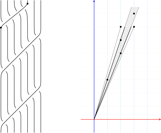
In total, (3)(a) holds for one of , and (3)(b) holds for the other. Applying the linear map exchanges with its mirror (see [Wu04, §4]). Thus, we may assume that (3)(a) holds for and (3)(b) for . We have for some , . Since , we obtain , and so . Hence
We deduce in turn that , , , , , , and . Since is the Farey sequence of fractions between and , the slope interval of is , and it has winding number . See Figure 4. These invariants specify . ∎
References
- [Ber] John Berge, Some knots with surgeries yielding lens spaces, Unpublished manuscript.
- [Ber91] by same author, The knots in which have nontrivial Dehn surgeries that yield , Topology Appl. 38 (1991), no. 1, 1–19.
- [BBCW12] Michel Boileau, Steven Boyer, Radu Cebanu, and Genevieve S. Walsh, Knot commensurability and the Berge conjecture, Geom. Topol. 16 (2012), no. 2, 625–664.
- [CGLS87] Marc Culler, C. McA. Gordon, J. Luecke, and Peter B. Shalen, Dehn surgery on knots, Ann. of Math. 125 (1987), no. 2, 237–300.
- [Gab90] David Gabai, -bridge braids in solid tori, Topology Appl. 37 (1990), no. 3, 221–235.
- [GMM05] Hiroshi Goda, Hiroshi Matsuda, and Takayuki Morifuji, Knot Floer homology of -knots, Geometriae Dedicata 112 (2005), no. 1, 197–214.
- [Hed11] Matthew Hedden, On Floer homology and the Berge conjecture on knots admitting lens space surgeries, Trans. Amer. Math. Soc. 363 (2011), no. 2, 949–968.
- [HLV14] Jennifer Hom, Tye Lidman, and Faramarz Vafaee, Berge-Gabai knots and L-space satellite operations, Algebr. Geom. Topol. 14 (2014), no. 6, 3745–3763.
- [Juh15] András Juhász, A survey of Heegaard Floer homology, New ideas in low dimensional topology, vol. 56, World Sci. Publ., Hackensack, NJ, 2015, pp. 237–296.
- [Krc] David Krcatovich, Private communication.
- [MZ01] William Menasco and Xingru Zhang, Notes on tangles, 2-handle additions and exceptional Dehn fillings, Pacific J. Math. 198 (2001), no. 1, 149–174.
- [OS04] Peter Ozsváth and Zoltán Szabó, Holomorphic disks and knot invariants, Adv. Math. 186 (2004), no. 1, 58–116.
- [OS05] by same author, On knot Floer homology and lens space surgeries, Topology 44 (2005), no. 6, 1281–1300.
- [Ras05] Jacob Rasmussen, Knot polynomials and knot homologies, Geometry and topology of manifolds, vol. 47, Amer. Math. Soc., Providence, RI, 2005, pp. 261–280.
- [RR15] Jacob Rasmussen and Sarah Dean Rasmussen, Floer simple manifolds and L-space intervals, To appear in Adv. Math., preprint (2015), arXiv:1508.05900.
- [Vaf15] Faramarz Vafaee, On the knot Floer homology of twisted torus knots, Int. Math. Res. Not. (2015), no. 15, 6516–6537.
- [Wu04] Ying-Qing Wu, The classification of Dehn fillings on the outer torus of a 1-bridge braid exterior which produce solid tori, Math. Ann. 330 (2004), no. 1, 1–15.