An Adaptive Test of Independence with Analytic Kernel Embeddings

Abstract

A new computationally efficient dependence measure, and an adaptive statistical test of independence, are proposed. The dependence measure is the difference between analytic embeddings of the joint distribution and the product of the marginals, evaluated at a finite set of locations (features). These features are chosen so as to maximize a lower bound on the test power, resulting in a test that is data-efficient, and that runs in linear time (with respect to the sample size n). The optimized features can be interpreted as evidence to reject the null hypothesis, indicating regions in the joint domain where the joint distribution and the product of the marginals differ most. Consistency of the independence test is established, for an appropriate choice of features. In real-world benchmarks, independence tests using the optimized features perform comparably to the state-of-the-art quadratic-time HSIC test, and outperform competing $\mathcal{O}(n)$ and $\mathcal{O}(n\log n)$ tests.

1 Introduction

We consider the design of adaptive, nonparametric statistical tests of dependence: that is, tests of whether a joint distribution $P_{xy}$ factorizes into the product of marginals $P_{x}P_{y}$. While classical tests of dependence, such as Pearson’s correlation and Kendall’s $\tau$, are able to detect monotonic relations between univariate variables, more modern tests can address complex interactions, for instance changes in variance of $X$ with the value of $Y$. Key to many recent tests is to examine covariance or correlation between data features. These interactions become significantly harder to detect, and the features are more difficult to design when the data reside in high dimensions.

A basic nonlinear dependence measure is the Hilbert-Schmidt Independence Criterion (HSIC), which is the Hilbert-Schmidt norm of the covariance operator between feature mappings of the random variables (Gretton et al., 2005, 2008). Each random variable $X$ and $Y$ is mapped to a respective reproducing kernel Hilbert space $\mathcal{H}_{k}$ and $\mathcal{H}_{l}$. For sufficiently rich mappings, the covariance operator norm is zero if and only if the variables are independent. A second basic nonlinear dependence measure is the smoothed difference between the characteristic function of the joint distribution, and that of the product of marginals. When a particular smoothing function is used, the statistic corresponds to the covariance between distances of X and Y variable pairs (Feuerverger, 1993; Székely et al., 2007; Székely and Rizzo, 2009), yielding a simple test statistic. It has been shown by Sejdinovic et al. (2013) that the distance covariance (and its generalization to semi-metrics) is an instance of HSIC for an appropriate choice of kernels. A disadvantage of these feature covariance statistics, however, is that they require quadratic time to compute (besides in the special case of the distance covariance with univariate real-valued variables, where Huo and Székely (2014) achieve an $\mathcal{O}(n\log n)$ cost). Moreover, the feature covariance statistics have intractable null distributions, and either a permutation approach or the solution of an expensive eigenvalue problem (e.g. Zhang et al., 2011) is required for consistent estimation of the quantiles. Several approaches were proposed by Zhang et al. (2016) to obtain faster tests along the lines of HSIC. These include computing HSIC on finite-dimensional feature mappings chosen as random Fourier features (RFFs) (Rahimi and Recht, 2008), a block-averaged statistic, and a Nyström approximation to the statistic. Key to each of these approaches is a more efficient computation of the statistic and its threshold under the null distribution: for RFFs, the null distribution is a finite weighted sum of $\chi^{2}$ variables; for the block-averaged statistic, the null distribution is asymptotically normal; for Nyström, either a permutation approach is employed, or the spectrum of the Nyström approximation to the kernel matrix is used in approximating the null distribution. Each of these methods costs significantly less than the $\mathcal{O}(n^{2})$ cost of the full HSIC (the cost is linear in $n$, but also depends quadratically on the number of features retained). A potential disadvantage of the Nyström and Fourier approaches is that the features are not optimized to maximize test power, but are chosen randomly. The block statistic performs worse than both, due to the large variance of the statistic under the null (which can be mitigated by observing more data).

In addition to feature covariances, correlation measures have also been developed in infinite dimensional feature spaces: in particular, Bach and Jordan (2002); Fukumizu et al. (2008) proposed statistics on the correlation operator in a reproducing kernel Hilbert space. While convergence has been established for certain of these statistics, their computational cost is high at $\mathcal{O}(n^{3})$, and test thresholds have relied on permutation. A number of much faster approaches to testing based on feature correlations have been proposed, however. For instance, Dauxois and Nkiet (1998) compute statistics of the correlation between finite sets of basis functions, chosen for instance to be step functions or low order B-splines. The cost of this approach is $\mathcal{O}(n)$. This idea was extended by Lopez-Paz et al. (2013), who computed the canonical correlation between finite sets of basis functions chosen as random Fourier features; in addition, they performed a copula transform on the inputs, with a total cost of $\mathcal{O}(n\log n)$. Finally, space partitioning approaches have also been proposed, based on statistics such as the KL divergence, however these apply only to univariate variables (Heller et al., 2016), or to multivariate variables of low dimension (Gretton and Györfi, 2010) (that said, these tests have other advantages of theoretical interest, notably distribution-independent test thresholds).

The approach we take is most closely related to HSIC on a finite set of features. Our simplest test statistic, the Finite Set Independence Criterion (FSIC), is an average of covariances of analytic functions (i.e., features) defined on each of $X$ and $Y$. A normalized version of the statistic (NFSIC) yields a distribution-independent asymptotic test threshold. We show that our test is consistent, despite a finite number of analytic features being used, via a generalization of arguments in Chwialkowski et al. (2015). As in recent work on two-sample testing by Jitkrittum et al. (2016), our test is adaptive in the sense that we choose our features on a held-out validation set to optimize a lower bound on the test power. The design of features for independence testing turns out to be quite different to the case of two-sample testing, however: the task is to find correlated feature pairs on the respective marginal domains, rather than attempting to find a single, high-dimensional feature representation for the entire $(x,y)$ (as we would need to do if we were comparing distributions $P_{xy}$ and $Q_{xy}$, rather than testing a specific property of $P_{xy}$). We demonstrate the performance of our tests on several challenging artificial and real-world datasets, including detection of dependence between music and its year of appearance, and between videos and captions. In these experiments, we outperform competing linear and $\mathcal{O}(n\log n)$ time tests.

2 Independence Criteria and Statistical Tests

We introduce two test statistics: first, the Finite Set Independence Criterion (FSIC), which builds on the principle that dependence can be measured in terms of the covariance between data features. Next, we propose a normalized version of this statistic (NFSIC), with a simpler asymptotic distribution when $P_{xy}=P_{x}P_{y}$. We show how to select features for the latter statistic to maximize a lower bound on the power of its corresponding statistical test.

2.1 The Finite Set Independence Criterion

We begin by introducing the Hilbert-Schmidt Independence Criterion (HSIC) as proposed in Gretton et al. (2005), since our unnormalized statistic is built along similar lines. Consider two random variables $X\in\mathcal{X}\subset\mathbb{R}^{d_{x}}$ and $Y\in\mathcal{Y}\subset\mathbb{R}^{d_{y}}$. Denote by $P_{xy}$ the joint distribution between $X$ and $Y$; $P_{x}$ and $P_{y}$ are the marginal distributions of $X$ and $Y$. Let $\otimes$ denote the tensor product, such that $\left(a\otimes b\right)c=a\left\langle b,c\right\rangle$. Assume that $k:\mathcal{X}\times\mathcal{X}\to\mathbb{R}$ and $l:\mathcal{Y}\times\mathcal{Y}\to\mathbb{R}$ are positive definite kernels associated with reproducing kernel Hilbert spaces (RKHS) $\mathcal{H}_{k}$ and $\mathcal{H}_{l}$, respectively. Let $\|\cdot\|_{HS}$ be the norm on the space of $\mathcal{H}_{l}\to\mathcal{H}_{k}$ Hilbert-Schmidt operators. Then, HSIC between $X$ and $Y$ is defined as

$$\mathrm{HSIC}(X,Y)=\big{\|}\mu_{xy}-\mu_{x}\otimes\mu_{y}\big{\|}_{\mathrm{HS}}^{2}$$

$$=\mathbb{E}_{(\mathbf{x},\mathbf{y}),(\mathbf{x}^{\prime},\mathbf{y}^{\prime})}\left[k(\mathbf{x},\mathbf{x}^{\prime})l(\mathbf{y},\mathbf{y}^{\prime})\right]$$

$$\quad+\mathbb{E}_{\mathbf{x}}\mathbb{E}_{\bm{\mathbf{x}^{\prime}}}[k(\mathbf{x},\mathbf{x}^{\prime})]\mathbb{E}_{\mathbf{y}}\mathbb{E}_{\mathbf{y}^{\prime}}[l(\mathbf{y},\mathbf{y}^{\prime})]$$

$$\quad-2\mathbb{E}_{(\mathbf{x},\mathbf{y})}\left[\mathbb{E}_{\mathbf{x}^{\prime}}[k(\mathbf{x},\mathbf{x}^{\prime})]\mathbb{E}_{\mathbf{y}^{\prime}}[l(\mathbf{y},\mathbf{y}^{\prime})]\right],$$ (1)

where $\mathbb{E}_{\mathbf{x}}:=\mathbb{E}_{\mathbf{x}\sim P_{x}}$, $\mathbb{E}_{\mathbf{y}}:=\mathbb{E}_{\mathbf{y}\sim P_{y}}$, $\mathbb{E}_{(\mathbf{x},\mathbf{y})}:=\mathbb{E}_{(\mathbf{x},\mathbf{y})\sim P_{xy}}$, and $\mathbf{x}^{\prime}$ is an independent copy of $\mathbf{x}$. The mean embedding of $P_{xy}$ belongs to the space of Hilbert-Schmidt operators from $\mathcal{H}_{l}$ to $\mathcal{H}_{k}$, $\mu_{xy}:=\int_{\mathcal{X}\times\mathcal{Y}}k(\mathbf{x},\cdot)\otimes l(\mathbf{y},\cdot)\thinspace\mathrm{d}P_{xy}(\mathbf{x},\mathbf{y})\in\mathrm{HS}(\mathcal{H}_{l},\mathcal{H}_{k})$, and the marginal mean embeddings are $\mu_{x}:=\int_{\mathcal{X}}k(\mathbf{x},\cdot)\thinspace\mathrm{d}P_{x}(\mathbf{x})\in\mathcal{H}_{k}$ and $\mu_{y}:=\int_{\mathcal{Y}}l(\mathbf{y},\cdot)\thinspace\mathrm{d}P_{y}(\mathbf{y})\in\mathcal{H}_{l}$ (Smola et al., 2007). Gretton et al. (2005, Theorem 4) show that if the kernels $k$ and $l$ are universal (Steinwart and Christmann, 2008) on compact domains $\mathcal{X}$ and $\mathcal{Y}$, then $\mathrm{HSIC}(X,Y)=0$ if and only if $X$ and $Y$ are independent. Alternatively, Gretton (2015) shows that it is sufficient for each of $k$ and $l$ to be characteristic to their respective domains (meaning that distribution embeddings are injective in each marginal domain: see Sriperumbudur et al. (2010)). Given a joint sample $\mathsf{Z}_{n}=\{(\mathbf{x}_{i},\mathbf{y}_{i})\}_{i=1}^{n}\sim P_{xy}$, an empirical estimator of HSIC can be computed in $\mathcal{O}(n^{2})$ time by replacing the population expectations in (1) with their corresponding empirical expectations based on $\mathsf{Z}_{n}$.

We now propose our new linear-time dependence measure, the Finite Set Independence Criterion (FSIC). Let $\mathcal{X}\subset\mathbb{R}^{d_{x}}$ and $\mathcal{Y}\subset\mathbb{R}^{d_{y}}$ be open sets. Define the empirical measure $\nu:=\frac{1}{J}\sum_{i=1}^{J}\delta_{(\mathbf{v}_{i},\mathbf{w}_{i})}$ over $J$ test locations $V_{J}:=\{(\mathbf{v}_{i},\mathbf{w}_{i})\}_{i=1}^{J}\subset\mathcal{X}\times\mathcal{Y}$ where $\delta_{\mathbf{t}}$ denotes the Dirac measure centered on $\mathbf{t}$, and $(\mathbf{v}_{i},\mathbf{w}_{i})$ are realizations from an absolutely continuous distribution (wrt the Lebesgue measure). Write $\mathbb{E}_{\mathbf{x}\mathbf{y}}$ for $\mathbb{E}_{(\mathbf{x},\mathbf{y})\sim P_{xy}}$. The idea is to see $\mu_{xy}(\mathbf{v},\mathbf{w})=\mathbb{E}_{\mathbf{x}\mathbf{y}}[k(\mathbf{x},\mathbf{v})l(\mathbf{y},\mathbf{w})],\mu_{x}(\mathbf{v})=\mathbb{E}_{\mathbf{x}}[k(\mathbf{x},\mathbf{v})]$ and $\mu_{y}(\mathbf{w})=\mathbb{E}_{\mathbf{y}}[l(\mathbf{y},\mathbf{w})]$ as smooth functions, and consider an $L^{2}(\mathcal{X}\times\mathcal{Y},\nu)$ distance between $\mu_{xy}$ and $\mu_{x}\mu_{y}$ instead of a Hilbert-Schmidt distance as in HSIC (Gretton et al., 2005). Let $\mu_{x}\mu_{y}(\mathbf{x},\mathbf{y}):=\mu_{x}(\mathbf{x})\mu_{y}(\mathbf{y})$. FSIC is defined as

$$\mathrm{FSIC}^{2}(X,Y):=\|\mu_{xy}-\mu_{x}\mu_{y}\|_{L^{2}(\mathcal{X}\times\mathcal{Y},\text{$\nu$})}^{2}$$

$$=\int_{\mathcal{X}}\int_{\mathcal{Y}}(\mu_{xy}(\mathbf{x},\mathbf{y})-\mu_{x}(\mathbf{x})\mu_{y}(\mathbf{y}))^{2}\thinspace\mathrm{d}\nu(\mathbf{x},\mathbf{y})$$

$$:=\frac{1}{J}\sum_{i=1}^{J}u(\mathbf{v}_{i},\mathbf{w}_{i})^{2}=\frac{1}{J}\|\mathbf{u}\|_{2}^{2},\text{ where }$$

$$u(\mathbf{v},\mathbf{w}):=\mu_{xy}(\mathbf{v},\mathbf{w})-\mu_{x}(\mathbf{v})\mu_{y}(\mathbf{w})$$

$$=\mathbb{E}_{\mathbf{x}\mathbf{y}}[k(\mathbf{x},\mathbf{v})l(\mathbf{y},\mathbf{w})]-\mathbb{E}_{\mathbf{x}}[k(\mathbf{x},\mathbf{v})]\mathbb{E}_{\mathbf{y}}[l(\mathbf{y},\mathbf{w})],$$ (2)

$$=\mathrm{cov_{\mathbf{x}\mathbf{y}}}[k(\mathbf{x},\mathbf{v}),l(\mathbf{y},\mathbf{w})],$$

and $\mathbf{u}:=(u(\mathbf{v}_{1},\mathbf{w}_{1}),\ldots,u(\mathbf{v}_{J},\mathbf{w}_{J}))^{\top}$.

Our first result in Proposition 2 states that $\mathrm{FSIC}(X,Y)$ almost surely defines a dependence measure for the random variables $X$ and $Y$, provided that the product kernel on the joint space $\mathcal{X}\times\mathcal{Y}$ is characteristic and analytic (see Definition 1).

Definition 1 (Analytic kernels (Chwialkowski et al., 2015)).

Let $\mathcal{X}$ be an open set in $\mathbb{R}^{d}$. A positive definite kernel $k:\mathcal{X}\times\mathcal{X}\to\mathbb{R}$ is said to be analytic on its domain $\mathcal{X}\times\mathcal{X}$ if for all $\mathbf{v}\in\mathcal{X}$, $f(\mathbf{x}):=k(\mathbf{x},\mathbf{v})$ is an analytic function on $\mathcal{X}$.

Assumption A.

The kernels $k:\mathcal{X}\times\mathcal{X}\to\mathbb{R}$ and $l:\mathcal{Y}\times\mathcal{Y}\to\mathbb{R}$ are bounded by $B_{k}$ and $B_{l}$ respectively, and the product kernel $g((\mathbf{x},\mathbf{y}),(\mathbf{x}^{\prime},\mathbf{y}^{\prime})):=k(\mathbf{x},\mathbf{x}^{\prime})l(\mathbf{y},\mathbf{y}^{\prime})$ is characteristic (Sriperumbudur et al., 2010, Definition 6), and analytic (Definition 1) on $(\mathcal{X}\times\mathcal{Y})\times(\mathcal{X}\times\mathcal{Y})$.

Proposition 2 (FSIC is a dependence measure).

Assume that

1. Assumption A holds.

2. The test locations $V_{J}=\{(\mathbf{v}_{i},\mathbf{w}_{i})\}_{i=1}^{J}$ are drawn from an absolutely continuous distribution.

Then, almost surely, $\mathrm{FSIC}(X,Y)=\frac{1}{\sqrt{J}}\|\mathbf{u}\|_{2}=0$ if and only if $X$ and $Y$ are independent.

Proof.

Since $g$ is characteristic, the mean embedding map $\Pi_{g}:P\mapsto\mathbb{E}_{(\mathbf{x},\mathbf{y})\sim P}[g((\mathbf{x},\mathbf{y}),\cdot)]$ is injective (Sriperumbudur et al., 2010, Section 3), where $P$ is a probability distribution on $\mathcal{X}\times\mathcal{Y}$. Since $g$ is analytic, by Lemma 10 (Appendix), $\mu_{xy}$ and $\mu_{x}\mu_{y}$ are analytic functions. Thus, Lemma 11 (Appendix, setting $\Lambda=\Pi_{g}$) guarantees that $\mathrm{FSIC}(X,Y)=0\iff P_{xy}=P_{x}P_{y}\iff X$ and $Y$ are independent almost surely. ∎

FSIC uses $\mu_{xy}$ as a proxy for $P_{xy}$, and $\mu_{x}\mu_{y}$ as a proxy for $P_{x}P_{y}$. Proposition 2 suggests that, to detect the dependence between $X$ and $Y$, it is sufficient to evaluate at a finite number of locations (defined by $V_{J}$) the difference of the population joint embedding $\mu_{xy}$ and the embedding of the product of the marginal distributions $\mu_{x}\mu_{y}$. A brief explanation to justify this property is as follows. If $P_{xy}=P_{x}P_{y}$, then $\rho(\mathbf{v},\mathbf{w}):=\mu_{xy}(\mathbf{v},\mathbf{w})-\mu_{x}\mu_{y}(\mathbf{v},\mathbf{w})$ is zero, and $\mathrm{FSIC}(X,Y)=0$ for any $V_{J}$. If $P_{xy}\neq P_{x}P_{y}$, then $\rho$ will not be a zero function, since the mean embedding map is injective (require the product kernel to be characteristic). Using the same argument as in Chwialkowski et al. (2015), since $k$ and $l$ are analytic, $\rho$ is also analytic, and the set of roots $R:=\{(\mathbf{v},\mathbf{w})\mid\rho(\mathbf{v},\mathbf{w})=0\}$ has Lebesgue measure zero. Thus, it is sufficient to draw $(\mathbf{v},\mathbf{w})$ from an absolutely continuous distribution, as we are guaranteed that $(\mathbf{v},\mathbf{w})\notin R$ giving $\mathrm{FSIC}(X,Y)>0$.

For FSIC to be a dependence measure, the product kernel is required to be characteristic and analytic. We next show in Proposition 3 that Gaussian kernels $k$ and $l$ yield such a product kernel.

Proposition 3 (A product of Gaussian kernels is characteristic and analytic).

Let $k(\mathbf{x},\mathbf{x}^{\prime})=\exp\left(-(\mathbf{x}-\mathbf{x}^{\prime})^{\top}\mathbf{A}(\mathbf{x}-\mathbf{x}^{\prime})\right)$ and $l(\mathbf{y},\mathbf{y}^{\prime})=\exp\left(-(\mathbf{y}-\mathbf{y}^{\prime})^{\top}\mathbf{B}(\mathbf{y}-\mathbf{y}^{\prime})\right)$ be Gaussian kernels on $\mathbb{R}^{d_{x}}\times\mathbb{R}^{d_{x}}$ and $\mathbb{R}^{d_{y}}\times\mathbb{R}^{d_{y}}$ respectively, for positive definite matrices $\mathbf{A}$ and $\mathbf{B}$. Then, $g((\mathbf{x},\mathbf{y}),(\mathbf{x}^{\prime},\mathbf{y}^{\prime}))=k(\mathbf{x},\mathbf{x}^{\prime})l(\mathbf{y},\mathbf{y}^{\prime})$ is characteristic and analytic on $(\mathbb{R}^{d_{x}}\times\mathbb{R}^{d_{y}})\times(\mathbb{R}^{d_{x}}\times\mathbb{R}^{d_{y}})$.

Proof (sketch).

The main idea is to use the fact a Gaussian kernel is analytic, and a product of Gaussian kernels is a Gaussian kernel on the pair of variables. See the full proof in Appendix D. ∎

Plug-in Estimator We now give an empirical estimator of FSIC. Assume that we observe a joint sample $\mathsf{Z}_{n}:=\{(\mathbf{x}_{i},\mathbf{y}_{i})\}_{i=1}^{n}\stackrel{{\scriptstyle i.i.d.}}{{\sim}}P_{xy}$. Unbiased estimators of $\mu_{xy}(\mathbf{v},\mathbf{w})$ and $\mu_{x}\mu_{y}(\mathbf{v},\mathbf{w})$ are $\hat{\mu}_{xy}(\mathbf{v},\mathbf{w}):=\frac{1}{n}\sum_{i=1}^{n}k(\mathbf{x}_{i},\mathbf{v})l(\mathbf{y}_{i},\mathbf{w})$ and $\widehat{\mu_{x}\mu_{y}}(\mathbf{v},\mathbf{w}):=\frac{1}{n(n-1)}\sum_{i=1}^{n}\sum_{j\neq i}k(\mathbf{x}_{i},\mathbf{v})l(\mathbf{y}_{j},\mathbf{w})$, respectively. A straightforward empirical estimator of $\mathrm{FSIC}^{2}$ is then given by

$$\widehat{\mathrm{FSIC^{2}}}(\mathsf{Z}_{n}) =\frac{1}{J}\sum_{i=1}^{J}\hat{u}(\mathbf{v}_{i},\mathbf{w}_{i})^{2},$$

$$\hat{u}(\mathbf{v},\mathbf{w}) :=\hat{\mu}_{xy}(\mathbf{v},\mathbf{w})-\widehat{\mu_{x}\mu_{y}}(\mathbf{v},\mathbf{w})$$ (3)

$$=\frac{2}{n(n-1)}\sum_{i<j}h_{(\mathbf{v},\mathbf{w})}((\mathbf{x}_{i},\mathbf{y}_{i}),(\mathbf{x}_{j},\mathbf{y}_{j})),$$ (4)

where $h_{(\mathbf{v},\mathbf{w})}((\mathbf{x},\mathbf{y}),(\mathbf{x}^{\prime},\mathbf{y}^{\prime})):=\frac{1}{2}(k(\mathbf{x},\mathbf{v})-k(\mathbf{x}^{\prime},\mathbf{v}))(l(\mathbf{y},\mathbf{w})-l(\mathbf{y}^{\prime},\mathbf{w}))$. For conciseness, we define $\hat{\mathbf{u}}:=(\hat{u}_{1},\ldots,\hat{u}_{J})^{\top}\in\mathbb{R}^{J}$ where $\hat{u}_{i}:=\hat{u}(\mathbf{v}_{i},\mathbf{w}_{i})$ so that $\widehat{\mathrm{FSIC^{2}}}(\mathsf{Z}_{n})=\frac{1}{J}\hat{\mathbf{u}}^{\top}\hat{\mathbf{u}}$.

$\widehat{\mathrm{FSIC^{2}}}$ can be efficiently computed in $\mathcal{O}((d_{x}+d_{y})Jn)$ time [see (3)], assuming that the runtime complexity of evaluating $k(\mathbf{x},\mathbf{v})$ is $\mathcal{O}(d_{x})$ and that of $l(\mathbf{y},\mathbf{w})$ is $\mathcal{O}(d_{y})$. The unbiasedness of $\widehat{\mu_{x}\mu_{y}}$ is necessary for $\eqref{eq:ustat}$ to be a U-statistic. This fact and the rewriting of $\widehat{\mathrm{FSIC^{2}}}$ in terms of $h_{(\mathbf{v},\mathbf{w})}((\mathbf{x},\mathbf{y}),(\mathbf{x}^{\prime},\mathbf{y}^{\prime}))$ will be exploited when the asymptotic distribution of $\hat{\mathbf{u}}$ is derived (Proposition 4).

Since $\mathrm{FSIC}$ satisfies $\mathrm{FSIC}(X,Y)=0\iff X\perp Y$, in principle its empirical estimator can be used as a test statistic for an independence test proposing a null hypothesis $H_{0}:$ “$X$ and $Y$ are independent” against an alternative $H_{1}:$ “$X$ and $Y$ are dependent”. The null distribution (i.e., distribution of the test statistic assuming that $H_{0}$ is true) is challenging to obtain, however and depends on the unknown $P_{xy}$. This prompts us to consider a normalized version of $\mathrm{FSIC}$ whose asymptotic null distribution of a convenient form. We first derive the asymptotic distribution of $\hat{\mathbf{u}}$ in Proposition 4, which we use to derive the normalized test statistic in Theorem 5. As a shorthand, we write $\mathbf{z}:=(\mathbf{x},\mathbf{y})$, and $\mathbf{t}:=(\mathbf{v},\mathbf{w})$.

Proposition 4 (Asymptotic distribution of $\hat{\mathbf{u}}$).

Define $\tilde{k}(\mathbf{x},\mathbf{v}):=k(\mathbf{x},\mathbf{v})-\mathbb{E}_{\mathbf{x}^{\prime}}k(\mathbf{x}^{\prime},\mathbf{v})$, and $\tilde{l}(\mathbf{y},\mathbf{w}):=l(\mathbf{y},\mathbf{w})-\mathbb{E}_{\mathbf{y}^{\prime}}l(\mathbf{y}^{\prime},\mathbf{w})$. Then, under both $H_{0}$ and $H_{1}$, for any fixed locations $\mathbf{t}$ and $\mathbf{t}^{\prime}$,

$$\mathrm{cov_{\mathbf{z}}}[\hat{u}(\mathbf{t}),\hat{u}(\mathbf{t}^{\prime})]\xrightarrow{n\to\infty}\mathrm{cov_{\mathbf{z}}}[\tilde{k}(\mathbf{x},\mathbf{v})\tilde{l}(\mathbf{y},\mathbf{w}),\tilde{k}(\mathbf{x},\mathbf{v}^{\prime})\tilde{l}(\mathbf{y},\mathbf{w}^{\prime})]$$

$$=\mathbb{E}_{\mathbf{x}\mathbf{y}}[\big{(}\tilde{k}(\mathbf{x},\mathbf{v})\tilde{l}(\mathbf{y},\mathbf{w})-u(\mathbf{t})\big{)}\big{(}\tilde{k}(\mathbf{x},\mathbf{v}^{\prime})\tilde{l}(\mathbf{y},\mathbf{w}^{\prime})-u(\mathbf{t}^{\prime})\big{)}],$$

where $u(\mathbf{v},\mathbf{w})$ is given in (2), and $\hat{u}(\mathbf{v},\mathbf{w})$ is defined in (4). Second, if $0<\mathrm{cov}_{\mathbf{z}}[\hat{u}(\mathbf{t}_{i}),\hat{u}(\mathbf{t}_{i})]<\infty$ for $i=1,\ldots,J$, then $\sqrt{n}(\hat{\mathbf{u}}-\mathbf{u})\stackrel{{\scriptstyle d}}{{\to}}\mathcal{N}(\mathbf{0},\bm{\Sigma})$ as $n\to\infty$, where $\Sigma_{ij}=\mathrm{cov}[\hat{u}(\mathbf{t}_{i}),\hat{u}(\mathbf{t}_{j})]$ and $\mathbf{u}:=(u(\mathbf{t}_{1}),\ldots,u(\mathbf{t}_{J}))^{\top}$.

Proof.

We first note that for a fixed $\mathbf{t}=(\mathbf{v},\mathbf{w})$, $\hat{u}(\mathbf{v},\mathbf{w})$ is a one-sample second-order U-statistic (Serfling, 2009, Section 5.1.3) with a U-statistic kernel $h_{\mathbf{t}}$ where $h_{\mathbf{t}}(\mathbf{a},\mathbf{b})=h_{\mathbf{t}}(\mathbf{b},\mathbf{a})$. Thus, by Kowalski and Tu (2008, Section 5.1, Theorem 1), it follows directly that $\mathrm{cov}[\hat{u}(\mathbf{t}),\hat{u}(\mathbf{t}^{\prime})]=4\mathrm{cov}_{\mathbf{z}}[\mathbb{E}_{\mathbf{a}}h_{\mathbf{t}}(\mathbf{z},\mathbf{a}),\mathbb{E}_{\mathbf{b}}h_{\mathbf{t}^{\prime}}(\mathbf{z},\mathbf{b})]$. Substituting $h_{\mathbf{t}}$ with its definition yields the first claim, where we note that $\mathbb{E}_{\mathbf{x}\mathbf{y}}[\tilde{k}(\mathbf{x},\mathbf{v})\tilde{l}(\mathbf{y},\mathbf{w})]=u(\mathbf{v},\mathbf{w})$.

For the second claim, since $\hat{\mathbf{u}}$ is a multivariate one-sample U-statistic, by Lehmann (1999, Theorem 6.1.6) and Kowalski and Tu (2008, Section 5.1, Theorem 1), it follows that $\sqrt{n}(\hat{\mathbf{u}}-\mathbf{u})\stackrel{{\scriptstyle d}}{{\to}}\mathcal{N}(\mathbf{0},\bm{\Sigma})$ as $n\to\infty$, where $\Sigma_{ij}=\mathrm{cov}[\hat{u}(\mathbf{t}_{i}),\hat{u}(\mathbf{t}_{j})]$. ∎

Recall from Proposition 2 that $\mathbf{u}=0$ holds almost surely under $H_{0}$. The asymptotic normality in the second claim of Proposition 4 implies that $n\widehat{\mathrm{FSIC^{2}}}=\frac{n}{J}\hat{\mathbf{u}}^{\top}\hat{\mathbf{u}}$ converges in distribution to a sum of $J$ dependent weighted $\chi^{2}$ random variables. The dependence comes from the fact that the coordinates $\hat{u}_{1}\ldots,\hat{u}_{J}$ of $\hat{\mathbf{u}}$ all depend on the sample $\mathsf{Z}_{n}$. This null distribution is not analytically tractable, and requires a large number of simulations to compute the rejection threshold $T_{\alpha}$ for a given significance value $\alpha$.

2.2 Normalized FSIC and Adaptive Test

For the purpose of an independence test, we will consider a normalized variant of $\widehat{\mathrm{FSIC^{2}}}$, which we call $\widehat{\mathrm{NFSIC^{2}}}$, whose tractable asymptotic null distribution is $\chi^{2}(J)$, the chi-squared distribution with $J$ degrees of freedom. We then show that the independence test defined by $\widehat{\mathrm{NFSIC^{2}}}$ is consistent. These results are given in Theorem 5.

Theorem 5 (Independence test using $\widehat{\mathrm{NFSIC^{2}}}$ is consistent).

Let $\hat{\bm{\Sigma}}$ be a consistent estimate of $\bm{\Sigma}$ based on the joint sample $\mathsf{Z}_{n}$. The $\widehat{\mathrm{NFSIC^{2}}}$ statistic is defined as $\hat{\lambda}_{n}:=n\hat{\mathbf{u}}^{\top}\left(\hat{\bm{\Sigma}}+\gamma_{n}\mathbf{I}\right)^{-1}\hat{\mathbf{u}}$ where $\gamma_{n}\geq 0$ is a regularization parameter. Assume that

1. Assumption A holds.

2. $\bm{\Sigma}$ is invertible almost surely with respect to $V_{J}=\{(\mathbf{v}_{i},\mathbf{w}_{i})\}_{i=1}^{J}$ drawn from an absolutely continuous distribution.

3. $\lim_{n\to\infty}\gamma_{n}=0$.

Then, for any $k,l$ and $V_{J}$ satisfying the assumptions,

1. Under $H_{0}$, $\hat{\lambda}_{n}\stackrel{{\scriptstyle d}}{{\to}}\chi^{2}(J)$ as $n\to\infty$.

2. Under $H_{1}$, for any $r\in\mathbb{R}$, $\lim_{n\to\infty}\mathbb{P}\left(\hat{\lambda}_{n}\geq r\right)=1$ almost surely. That is, the independence test based on $\widehat{\mathrm{NFSIC^{2}}}$ is consistent.

Proof (sketch) .

Under $H_{0}$, $n\hat{\mathbf{u}}^{\top}(\hat{\bm{\Sigma}}+\gamma_{n}\mathbf{I})^{-1}\hat{\mathbf{u}}$ asymptotically follows $\chi^{2}(J)$ because $\sqrt{n}\hat{\mathbf{u}}$ is asymptotically normally distributed (see Proposition 4). Claim 2 builds on the result in Proposition 2 stating that $\mathbf{u}\neq 0$ under $H_{1}$; it follows using the convergence of $\hat{\mathbf{u}}$ to $\mathbf{u}$. The full proof can be found in Appendix E. ∎

Theorem 5 states that if $H_{1}$ holds, the statistic can be arbitrarily large as $n$ increases, allowing $H_{0}$ to be rejected for any fixed threshold. Asymptotically the test threshold $T_{\alpha}$ is given by the $(1-\alpha)$-quantile of $\chi^{2}(J)$ and is independent of $n$. The assumption on the consistency of $\hat{\mathbf{\Sigma}}$ is required to obtain the asymptotic chi-squared distribution. The regularization parameter $\gamma_{n}$ is to ensure that $(\hat{\mathbf{\Sigma}}+\gamma_{n}\mathbf{I})^{-1}$ can be stably computed. In practice, $\gamma_{n}$ requires no tuning, and can be set to be a very small constant.

The next proposition states that the computational complexity of the $\widehat{\mathrm{NFSIC^{2}}}$ estimator is linear in both the input dimension and sample size, and that it can be expressed in terms of the $\mathbf{K=}[K{}_{ij}]=[k(\mathbf{v}_{i},\mathbf{x}_{j})]\in\mathbb{R}^{J\times n},\mathbf{L}=[L_{ij}]=[l(\mathbf{w}_{i},\mathbf{y}_{j})]\in\mathbb{R}^{J\times n}$ matrices.

Proposition 6 (An empirical estimator of $\widehat{\mathrm{NFSIC^{2}}}$).

Let $\bm{1}_{n}:=(1,\ldots,1)^{\top}\in\mathbb{R}^{n}$. Denote by $\circ$ the element-wise matrix product. Then,

1. $\hat{\mathbf{u}}=\frac{\left(\mathbf{K}\circ\mathbf{L}\right)\bm{1}_{n}}{n-1}-\frac{\left(\mathbf{K}\bm{1}_{n}\right)\circ\left(\mathbf{L}\bm{1}_{n}\right)}{n(n-1)}$.

2. A consistent estimator for $\bm{\Sigma}$ is $\hat{\bm{\Sigma}}=\frac{\Gamma\Gamma^{\top}}{n}$ where

   $$\Gamma :=(\mathbf{K}-n^{-1}\mathbf{K}\bm{1}_{n}\bm{1}_{n}^{\top})\circ(\mathbf{L}-n^{-1}\mathbf{L}\bm{1}_{n}\bm{1}_{n}^{\top})-\hat{\mathbf{u}}^{b}\bm{1}_{n}^{\top},$$

   $$\hat{\mathbf{u}}^{b} =n^{-1}\left(\mathbf{K}\circ\mathbf{L}\right)\bm{1}_{n}-n^{-2}\left(\mathbf{K}\bm{1}_{n}\right)\circ\left(\mathbf{L}\bm{1}_{n}\right).$$

Assume that the complexity of the kernel evaluation is linear in the input dimension. Then the test statistic $\hat{\lambda}_{n}=n\hat{\mathbf{u}}^{\top}\left(\hat{\bm{\Sigma}}+\gamma_{n}\mathbf{I}\right)^{-1}\hat{\mathbf{u}}$ can be computed in $\mathcal{O}(J^{3}+J^{2}n+(d_{x}+d_{y})Jn)$ time.

Proof (sketch).

Claim 1 for $\hat{\mathbf{u}}$ is straightforward. The expression for $\hat{\mathbf{\Sigma}}$ in claim 2 follows directly from the asymptotic covariance expression in Proposition 4. The consistency of $\hat{\mathbf{\Sigma}}$ can be obtained by noting that the finite sample bound for $\mathbb{P}(\|\hat{\mathbf{\Sigma}}-\mathbf{\Sigma}\|_{F}>t)$ decreases as $n$ increases. This is implicitly shown in Appendix F.2.2 and its following sections. ∎

Although the dependency of the estimator on $J$ is cubic, we empirically observe that only a small value of $J$ is required (see Section 3). The number of test locations $J$ relates to the number of regions in $\mathcal{X}\times\mathcal{Y}$ of $p_{xy}$ and $p_{x}p_{y}$ that differ (see Figure 1). In particular, $J$ need not increase with $n$ for test consistency.

Our final theoretical result gives a lower bound on the test power of $\widehat{\mathrm{NFSIC^{2}}}$ i.e., the probability of correctly rejecting $H_{0}$. We will use this lower bound as the objective function to determine $V_{J}$ and the kernel parameters. Let $\|\cdot\|_{F}$ be the Frobenius norm.

Theorem 7 (A lower bound on the test power).

Let $\mathrm{NFSIC^{2}}(X,Y):=\lambda_{n}:=n\mathbf{u}^{\top}\bm{\Sigma}^{-1}\mathbf{u}$. Let $\mathcal{K}$ be a kernel class for $k$, $\mathcal{L}$ be a kernel class for $l$, and $\mathcal{V}$ be a collection with each element being a set of $J$ locations. Assume that

1. There exist finite $B_{k}$ and $B_{l}$ such that $\sup_{k\in\mathcal{K}}\sup_{\mathbf{x},\mathbf{x}^{\prime}\in\mathcal{X}}|k(\mathbf{x},\mathbf{x}^{\prime})|\leq B_{k}$ and $\sup_{l\in\mathcal{L}}\sup_{\mathbf{y},\mathbf{y}^{\prime}\in\mathcal{Y}}|l(\mathbf{y},\mathbf{y}^{\prime})|\leq B_{l}$.

2. $\tilde{c}:=\sup_{k\in\mathcal{K}}\sup_{l\in\mathcal{L}}\sup_{V_{J}\in\mathcal{V}}\|\bm{\Sigma}^{-1}\|_{F}<\infty$.

Then, for any $k\in\mathcal{K},l\in\mathcal{L},V_{J}\in\mathcal{V}$, and $\lambda_{n}\geq r$, the test power satisfies $\mathbb{P}\left(\hat{\lambda}_{n}\geq r\right)\geq L(\lambda_{n})$ where

$$L(\lambda_{n}) =1-62e^{-\xi_{1}\gamma_{n}^{2}(\lambda_{n}-r)^{2}/n}-2e^{-\lfloor 0.5n\rfloor(\lambda_{n}-r)^{2}/\left[\xi_{2}n^{2}\right]}$$

$$-2e^{-\left[(\lambda_{n}-r)\gamma_{n}(n-1)/3-\xi_{3}n-c_{3}\gamma_{n}^{2}n(n-1)\right]^{2}/\left[\xi_{4}n^{2}(n-1)\right]},$$

$\lfloor\cdot\rfloor$ is the floor function, $\xi_{1}:=\frac{1}{3^{2}c_{1}^{2}J^{2}B^{*}}$, $\xi_{2}:=72c_{2}^{2}JB^{2}$, $B:=B_{k}B_{l}$, $\xi_{3}:=8c_{1}B^{2}J$, $c_{3}:=4B^{2}J\tilde{c}^{2}$, $\xi_{4}:=2^{8}B^{4}J^{2}c_{1}^{2}$, $c_{1}:=4B^{2}J\sqrt{J}\tilde{c}$, $c_{2}:=4B\sqrt{J}\tilde{c}$, and $B^{*}$ is a constant depending on only $B_{k}$ and $B_{l}$. Moreover, for sufficiently large fixed $n$, $L(\lambda_{n})$ is increasing in $\lambda_{n}$.

We provide the proof in Appendix F. To put Theorem 7 into perspective, let $\theta_{x}$ and $\theta_{y}$ be the parameters of the kernels $k$ and $l$, respectively. We denote by $\theta=\{\theta_{x},\theta_{y},V_{J}\}$ the collection of all tuning parameters of the test. Assume that $\mathcal{K}=\left\{(\mathbf{x},\mathbf{v})\mapsto\exp\left(-\frac{\|\mathbf{x}-\mathbf{v}\|^{2}}{2\sigma_{x}^{2}}\right)\mid\sigma_{x}^{2}\in[\sigma_{x,l}^{2},\sigma_{x,u}^{2}]\right\}=:\mathcal{K}_{g}$ for some $0<\sigma_{x,l}^{2}<\sigma_{x,u}^{2}<\infty$ and $\mathcal{L}=\left\{(\mathbf{y},\mathbf{w})\mapsto\exp\left(-\frac{\|\mathbf{y}-\mathbf{w}\|^{2}}{2\sigma_{y}^{2}}\right)\mid\sigma_{y}^{2}\in[\sigma_{y,l}^{2},\sigma_{y,u}^{2}]\right\}=:\mathcal{L}_{g}$ for some $0<\sigma_{y,l}^{2}<\sigma_{y,u}^{2}<\infty$ are Gaussian kernel classes. Then, in Theorem 7, $B=B_{k}=B_{l}=1$, and $B^{*}=2$. The assumption $\tilde{c}<\infty$ is a technical condition to guarantee that the test power lower bound is finite for all $\theta$ defined by the feasible sets $\mathcal{K},\mathcal{L},$ and $\mathcal{V}$. Let $\mathcal{V}_{\epsilon,r}:=\big{\{}V_{J}\mid\|\mathbf{v}_{i}\|^{2},\|\mathbf{w}_{i}\|^{2}\leq r\text{ and }\|\mathbf{v}_{i}-\mathbf{v}_{j}\|_{2}^{2}+\|\mathbf{w}_{i}-\mathbf{w}_{j}\|_{2}^{2}\geq\epsilon,\text{ for all }i\neq j\big{\}}$. If we set $\mathcal{K}=\mathcal{K}_{g},\mathcal{L}=\mathcal{L}_{g},$ and $\mathcal{V}=\mathcal{V}_{\epsilon,r}$ for some $\epsilon,r>0$, then $\tilde{c}<\infty$ as $\mathcal{K}_{g},\mathcal{L}_{g},$ and $\mathcal{V}_{\epsilon,r}$ are compact. In practice, these conditions do not necessarily create restrictions as they almost always hold implicitly. We show in Appendix C that the objective function used to choose $V_{J}$ will discourage any two locations to be in the same neighborhood.

Parameter Tuning The test power lower bound $L(\lambda_{n})$ in Theorem 7 is a function of $\lambda_{n}=n\mathbf{u}^{\top}\mathbf{\Sigma}^{-1}\mathbf{u}$ which is the population counterpart of the test statistic $\hat{\lambda}_{n}$. As in FSIC, it can be shown that $\lambda_{n}=0$ if and only if $X$ are $Y$ are independent (from Proposition 2). If $X$ and $Y$ are dependent, then $\lambda_{n}>0$. According to Theorem 7, for a sufficiently large $n$, the test power lower bound is increasing in $\lambda_{n}$. One can therefore think of $\lambda_{n}$ (a function of $\theta$) as representing how easily the test rejects $H_{0}$ given a problem $P_{xy}$. The higher the $\lambda_{n}$, the greater the lower bound on the test power, and thus the more likely it is that the test will reject $H_{0}$ when it is false.

In light of this reasoning, we propose setting $\theta$ to $\theta^{*}=\arg\max_{\theta}\lambda_{n}$. That this procedure is also valid under $H_{0}$ can be seen as follows. Under $H_{0}$, $\theta^{*}=\arg\max_{\theta}0$ will be arbitrary. Since Theorem 7 guarantees that $\hat{\lambda}_{n}\stackrel{{\scriptstyle d}}{{\to}}\chi^{2}(J)$ as $n\to\infty$ for any $\theta$, the asymptotic null distribution does not change by using $\theta^{*}$. In practice, $\lambda_{n}$ is a population quantity which is unknown. We propose dividing the sample $\mathsf{Z}_{n}$ into two disjoint sets: training and test sets. The training set is used to optimize for $\theta^{*}$, and the test set is used for the actual independence test with the optimized $\theta^{*}$. The splitting is to guarantee the independence of $\theta^{*}$ and the test sample, which is an assumption of Theorem 5.

To better under $\widehat{\mathrm{NFSIC^{2}}}$, we visualize $\hat{\mu}_{xy}(\mathbf{v},\mathbf{w}),\widehat{\mu_{x}\mu_{y}}(\mathbf{v},\mathbf{w})$ and $\hat{\mathbf{\Sigma}}(\mathbf{v},\mathbf{w})$ as a function of one test location $(\mathbf{v},\mathbf{w})$ on a simple toy problem. In this problem, $Y=-X+Z$ where $Z\sim\mathcal{N}(0,0.3^{2})$. As we consider only one location $(J=1)$, $\hat{\mathbf{\Sigma}}(\mathbf{v},\mathbf{w})$ is a scalar. The statistic can be written as $\hat{\lambda}_{n}=n\frac{\left(\hat{\mu}_{xy}(\mathbf{v},\mathbf{w})-\widehat{\mu_{x}\mu_{y}}(\mathbf{v},\mathbf{w})\right)^{2}}{\hat{\mathbf{\Sigma}}(\mathbf{v},\mathbf{w})}$. These components are shown in Figure 1, where we use Gaussian kernels for both $X$ and $Y$, and the horizontal and vertical axes correspond to $\mathbf{v}\in\mathbb{R}$ and $\mathbf{w}\in\mathbb{R}$, respectively.

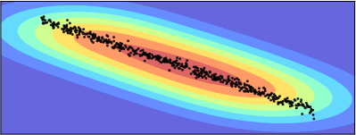
(a) $\hat{\mu}_{xy}(\mathbf{v},\mathbf{w})$

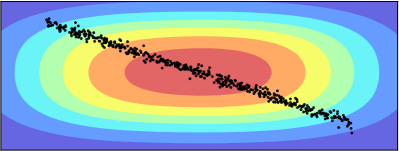
(b) $\widehat{\mu_{x}\mu_{y}}(\mathbf{v},\mathbf{w})$

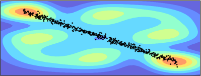
(c) $\widehat{\mathbf{\Sigma}}(\mathbf{v},\mathbf{w})$

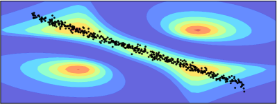
(d) Statistic $\hat{\lambda}_{n}(\mathbf{v},\mathbf{w})$

Figure 1: Illustration of $\widehat{\mathrm{NFSIC^{2}}}$.

Intuitively, $\hat{u}(\mathbf{v},\mathbf{w})=\hat{\mu}_{xy}(\mathbf{v},\mathbf{w})-\widehat{\mu_{x}\mu_{y}}(\mathbf{v},\mathbf{w})$ captures the difference of the joint distribution and the product of the marginals as a function of $(\mathbf{v},\mathbf{w})$. Squaring $\hat{u}(\mathbf{v},\mathbf{w})$ and dividing it by the variance shown in Figure 1c gives the statistic (also the parameter tuning objective) shown in Figure 1d. The latter figure suggests that the parameter tuning objective function can be non-convex. However, we note that the non-convexity arises since there are multiple ways to detect the difference between the joint distribution and the product of the marginals. In this case, the lower left and upper right regions equally indicate the largest difference.

3 Experiments

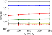
(a) SG $(\alpha=0.05)$

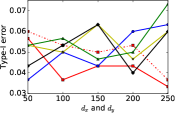
(b) SG $(\alpha=0.05)$

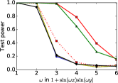
(c) Sin

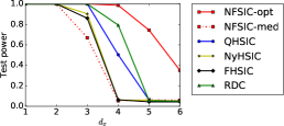
(d) GSign

Figure 2: (a): Runtime. (b): Probability of rejecting $H_{0}$ as problem parameters vary. Fix $n=4000$.

In this section, we empirically study the performance of the proposed method on both toy (Section 3.1) and real-life problems (Section 3.2). Our interest is in the performance of linear-time tests on challenging problems which require a large sample size to be able to accurately reveal the dependence. All the code is available at https://github.com/wittawatj/fsic-test.

We compare the proposed NFSIC with optimization (NFSIC-opt) to five multivariate nonparametric tests. The $\widehat{\mathrm{NFSIC^{2}}}$ test without optimization (NFSIC-med) acts as a baseline, allowing the effect of parameter optimization to be clearly seen. For pedagogical reason, we consider the original HSIC test of Gretton et al. (2005) denoted by QHSIC, which is a quadratic-time test. Nyström HSIC (NyHSIC) uses a Nyström approximation to the kernel matrices of $X$ and $Y$ when computing the HSIC statistic. FHSIC is another variant of HSIC in which a random Fourier feature approximation (Rahimi and Recht, 2008) to the kernel is used. NyHSIC and FHSIC are studied in Zhang et al. (2016) and can be computed in $\mathcal{O}(n)$, with quadratic dependency on the number of inducing points in NyHSIC, and quadratic dependency in the number of random features in FHSIC. Finally, the Randomized Dependence Coefficient (RDC) proposed in Lopez-Paz et al. (2013) is also considered. The RDC can be seen as the primal form (with random Fourier features) of the kernel canonical correlation analysis of Bach and Jordan (2002) on copula-transformed data. We consider RDC as a linear-time test even though preprocessing by an empirical copula transform costs $\mathcal{O}((d_{x}+d_{y})n\log n)$.

We use Gaussian kernel classes $\mathcal{K}_{g}$ and $\mathcal{L}_{g}$ for both $X$ and $Y$ in all the methods. Except NFSIC-opt, all other tests use full sample to conduct the independence test, where the Gaussian widths $\sigma_{x}$ and $\sigma_{y}$ are set according to the widely used median heuristic i.e., $\sigma_{x}=\mathrm{median}\left(\left\{\|\mathbf{x}_{i}-\mathbf{x}_{j}\|_{2}\mid 1\leq i<j\leq n\right\}\right)$, and $\sigma_{y}$ is set in the same way using $\{\mathbf{y}_{i}\}_{i=1}^{n}$. The $J$ locations for NFSIC-med are randomly drawn from the standard multivariate normal distribution in each trial. For a sample of size $n$, NFSIC-opt uses half the sample for parameter tuning, and the other disjoint half for the test. We permute the sample 300 times in RDC and HSIC to simulate from the null distribution and compute the test threshold. The null distributions for FHSIC and NyHSIC are given by a finite sum of weighted $\chi^{2}(1)$ random variables given in Eq. 8 of Zhang et al. (2016). Unless stated otherwise, we set the test threshold of the two NFSIC tests to be the $(1-\alpha)$-quantile of $\chi^{2}(J)$. To provide a fair comparison, we set $J=10$, use 10 inducing points in NyHSIC, and 10 random Fourier features in FHSIC and RDC.

Optimization of NFSIC-opt The parameters of NFSIC-opt are $\sigma_{x},\sigma_{y},$ and $J$ locations of size $(d_{x}+d_{y})J$. We treat all the parameters as a long vector in $\mathbb{R}^{2+(d_{x}+d_{y})J}$ and use gradient ascent to optimize $\hat{\lambda}_{n/2}$. We observe that initializing $V_{J}$ by randomly picking $J$ points from the training sample yields good performance. The regularization parameter $\gamma_{n}$ in NFSIC is fixed to a small value, and is not optimized. It is worth emphasizing that the complexity of the optimization procedure is still linear in $n$.

Since FSIC, NyHFSIC and RDC rely on a finite-dimensional kernel approximation, these tests are consistent only if both the number of features increases with $n$. By constrast, the proposed NFSIC requires only $n$ to go to infinity to achieve consistency i.e., $J$ can be fixed. We refer the reader to Appendix C for a brief investigation of the test power vs. increasing $J$. The test power does not necessarily monotonically increase with $J$.

3.1 Toy Problems

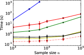
(a) SG. $d_{x}=d_{y}=250$.

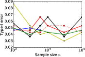
(b) SG. $d_{x}=d_{y}=250$.

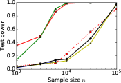
(c) Sin. $\omega=4$.

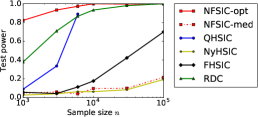
(d) GSign. $d_{x}=4$.

Figure 3: (a) Runtime. (b): Probability of rejecting $H_{0}$ as $n$ increases in the toy problems.

We consider three toy problems: Same Gaussian (SG), Sinusoid (Sin), and Gaussian Sign (GSign).

1. Same Gaussian (SG). The two variables are independently drawn from the standard multivariate normal distribution i.e., $X\sim\mathcal{N}(\mathbf{0},\mathbf{I}_{d_{x}})$ and $Y\sim\mathcal{N}(\mathbf{0},\mathbf{I}_{d_{y}})$ where $\mathbf{I}_{d}$ is the $d\times d$ identity matrix. This problem represents a case in which $H_{0}$ holds.

2. Sinusoid (Sin). Let $p_{xy}$ be the probability density of $P_{xy}$. In the Sinusoid problem, the dependency of $X$ and $Y$ is characterized by $(X,Y)\sim p_{xy}(x,y)\propto 1+\sin(\omega x)\sin(\omega y),$ where the domains of $\mathcal{X},\mathcal{Y}=(-\pi,\pi)$ and $\omega$ is the frequency of the sinusoid. As the frequency $\omega$ increases, the drawn sample becomes more similar to a sample drawn from $\mathrm{Uniform}((-\pi,\pi)^{2})$. That is, the higher $\omega$, the harder to detect the dependency between $X$ and $Y$. This problem was studied in Sejdinovic et al. (2013). Plots of the density for a few values of $\omega$ are shown in Figures 6 and 7 in the appendix. The main characteristic of interest in this problem is the local change in the density function.

3. Gaussian Sign (GSign). In this problem, $Y=|Z|\prod_{i=1}^{d_{x}}\mathrm{sgn}(X_{i}),$ where $X\sim\mathcal{N}(\mathbf{0},\mathbf{I}_{d_{x}})$, $\mathrm{sgn}(\cdot)$ is the sign function, and $Z\sim\mathcal{N}(0,1)$ serves as a source of noise. The full interaction of $X=(X_{1},\ldots,X_{d_{x}})$ is what makes the problem challenging. That is, $Y$ is dependent on $X$, yet it is independent of any proper subset of $\{X_{1},\ldots,X_{d}\}$. Thus, simultaneous consideration of all the coordinates of $X$ is required to successfully detect the dependency.

We fix $n=4000$ and vary the problem parameters. Each problem is repeated for 300 trials, and the sample is redrawn each time. The significance level $\alpha$ is set to 0.05. The results are shown in Figure 2. It can be seen that in the SG problem (Figure 2b) where $H_{0}$ holds, all the tests achieve roughly correct type-I errors at $\alpha=0.05$. In the Sin problem, NFSIC-opt achieves the highest test power for all considered $\omega=1,\ldots,6$, highlighting its strength in detecting local changes in the joint density. The performance of NFSIC-med is significantly lower than that of NFSIC-opt. This phenomenon clearly emphasizes the importance of the optimization to place the locations at the relevant regions in $\mathcal{X}\times\mathcal{Y}$. RDC has a remarkably high performance in both Sin and GSign (Figure 2c, 2d) despite no parameter tuning. Interestingly, both NFSIC-opt and RDC outperform the quadratic-time QHSIC in these two problems. The ability to simultaneously consider interacting features of NFSIC-opt is indicated by its superior test power in GSign, especially at the challenging settings of $d_{x}=5,6$. An average trial runtime for each test in the SG problem is shown in Figure 2a. We observe that the runtime does not increase with dimension, as the complexity of all the tests is linear in the dimension of the input. All the tests are implemented in Python using a common SciPy Stack.

To investigate the sample efficiency of all the tests, we fix $d_{x}=d_{y}=250$ in SG, $\omega=4$ in Sin, $d_{x}=4$ in GSign, and increase $n$. Figure 3 shows the results. The quadratic dependency on $n$ in QHSIC makes it infeasible both in terms of memory and runtime to consider $n$ larger than 6000 (Figure 3a). In constrast, although not the most time-efficient, NFSIC-opt has the highest sample-efficiency for GSign, and for Sin in the low-sample regime, significantly outperforming QHSIC. Despite the small additional overhead from the optimization, we are yet able to conduct an accurate test with $n=10^{5},d_{x}=d_{y}=250$ in less than $100$ seconds. We observe in Figure 3b that the two NFSIC variants have correct type-I errors across all sample sizes, indicating that the asymptotic null distribution approximately holds by the time $n$ reaches 1000. We recall from Theorem 5 that the NFSIC test with random test locations will asymptotically reject $H_{0}$ if it is false. A demonstration of this property is given in Figure 3c, where the test power of NFSIC-med eventually reaches 1 with $n$ higher than $10^{5}$.

3.2 Real Problems

We now examine the performance of our proposed test on real problems.

Million Song Data (MSD) We consider a subset of the Million Song Data (Bertin-Mahieux et al., 2011), in which each song $(X)$ out of 515,345 is represented by 90 features, of which 12 features are timbre average (over all segments) of the song, and 78 features are timbre covariance. Most of the songs are western commercial tracks from 1922 to 2011. The goal is to detect the dependency between each song and its year of release $(Y)$. We set $\alpha=0.01$, and repeat for 300 trials where the full sample is randomly subsampled to $n$ points in each trial. Other settings are the same as in the toy problems. To make sure that the type-I error is correct, we use the permutation approach in the NFSIC tests to compute the threshold. Figure 4b shows the test powers as $n$ increases from 500 to 2000. To simulate the case where $H_{0}$ holds in the problem, we permute the sample to break the dependency of $X$ and $Y$. The results are shown in Figure 5 in the appendix.

(a)

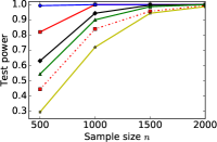
(b) (a) MSD problem.

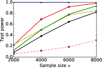
(c) (b) Videos & Captions problem.

Figure 4: Probability of rejecting $H_{0}$ as $n$ increases in the two real problems. $\alpha=0.01$.

Evidently, NFSIC-opt has the highest test power among all the linear-time tests for all the sample sizes. Its test power is second to only QHSIC. We recall that NFSIC-opt uses half of the sample for parameter tuning. Thus, at $n=500$, the actual sample for testing is 250, which is relatively small. The fact that there is a vast power gain from 0.4 (NFSIC-med) to 0.8 (NFSIC-opt) at $n=500$ suggests that the optimization procedure can perform well even at a lower sample sizes.

Videos and Captions Our last problem is based on the VideoStory46K dataset (Habibian et al., 2014). The dataset contains 45,826 Youtube videos $(X)$ of an average length of roughly one minute, and their corresponding text captions $(Y)$ uploaded by the users. Each video is represented as a $d_{x}=2000$ dimensional Fisher vector encoding of motion boundary histograms (MBH) descriptors of Wang and Schmid (2013). Each caption is represented as a bag of words with each feature being the frequency of one word. After filtering only words which occur in at least six video captions, we obtain $d_{y}=1878$ words. We examine the test powers as $n$ increases from $2000$ to $8000$. The results are given in Figure 4. The problem is sufficiently challenging that all linear-time tests achieve a low power at $n=2000$. QHSIC performs exceptionally well on this problem, achieving a maximum power throughout. NFSIC-opt has the highest sample efficiency among the linear-time tests, showing that the optimization procedure is also practical in a high dimensional setting.

Acknowledgement

We thank the Gatsby Charitable Foundation for the financial support. The major part of this work was carried out while Zoltán Szabó was a research associate at the Gatsby Computational Neuroscience Unit, University College London.

Appendix A Type-I Errors

In this section, we show that all the tests have correct type-I errors (i.e., the probability of reject $H_{0}$ when it is true) in real problems. We permute the joint sample so that the dependency is broken to simulate cases in which $H_{0}$ holds. The results are shown in Figure 5.

(a)

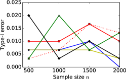
(b) (a) MSD problem (permuted).

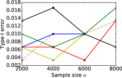
(c) (a) Videos & Captions problem with shuffled sample.

Figure 5: Probability of rejecting $H_{0}$ as $n$ increases in the Million Song problem. $\alpha=0.01$.

Appendix B Redundant Test Locations

Here, we provide a simple illustration to show that two locations $\mathbf{t}_{1}=(\mathbf{v}_{1},\mathbf{w}_{1})$ and $\mathbf{t}_{2}=(\mathbf{v}_{2},\mathbf{w}_{2})$ which are too close to each other will reduce the optimization objective. We consider the Sinusoid problem described in Section 3.1 with $\omega=1$, and use $J=2$ test locations. In Figure 6, $\mathbf{t}_{1}$ is fixed at the red star, while $\mathbf{t}_{2}$ is varied along the horizontal line. The objective value $\hat{\lambda}_{n}$ as a function of $(\mathbf{t}_{1},\mathbf{t}_{2})$ is shown in the bottom figure. It can be seen that $\hat{\lambda}_{n}$ decreases sharply when $\mathbf{t}_{2}$ is in the neighborhood of $\mathbf{t}_{1}$. This property implies that two locations which are too close will not maximize the objective function (i.e., the second feature contains no additional information when it matches the first). For $J>2$, the objective sharply decreases if any two locations are in the same neighborhood.

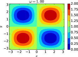
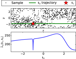
Figure 6: Plot of optimization objective values as location $\mathbf{t}_{2}$ moves along the green line. The objective sharply drops when the two locations are in the same neighborhood.

Appendix C Test Power vs. $J$

It might seem intuitive that as the number of locations $J$ increases, the test power should also increase. Here, we empirically show that this statement is not always true. Consider the Sinusoid toy example described in Section 3.1 with $\omega=2$ (also see the left figure of Figure 7). By construction, $X$ and $Y$ are dependent in this problem. We run NFSIC test with a sample size of $n=800$, varying $J$ from $1$ to $600$. For each value of $J$, the test is repeated for 500 times. In each trial, the sample is redrawn and the $J$ test locations are drawn from $\mathrm{Uniform}((-\pi,\pi)^{2})$. There is no optimization of the test locations. We use Gaussian kernels for both $X$ and $Y$, and use the median heuristic to set the Gaussian widths to 1.8. Figure 7 shows the test power as $J$ increases.

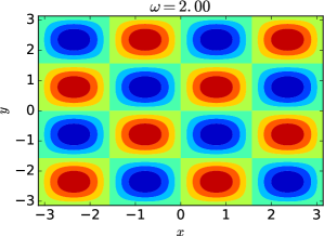
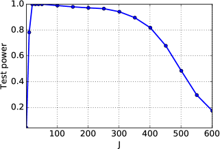
Figure 7: The Sinusoid problem and the plot of test power vs. the number of test locations.

We observe that the test power does not monotonically increase as $J$ increases. When $J=1$, the difference of $p_{xy}$ and $p_{x}p_{y}$ cannot be adequately captured, resulting in a low power. The power increases rapidly to roughly 0.8 at $J=10$, and stays at the maximum until about $J=100$. Then, the power starts to drop sharply when $J$ is higher than $400$ in this problem.

Unlike random Fourier features, the number of test locations in NFSIC is not the number of Monte Carlo particles used to approximate an expectation. There is a tradeoff: if the test locations are in key regions (i.e., regions in which there is a big difference between $p_{xy}$ and $p_{x}p_{y}$), then they increase power; yet the statistic gains in variance (thus reducing test power) as $J$ increases. As can be seen in Figure 7, there are eight key regions (in blue) that can reveal the difference of $p_{xy}$ and $p_{x}p_{y}$. Using an unnecessarily high $J$ not only makes the covariance matrix $\hat{\mathbf{\Sigma}}$ harder to estimate accurately, it also increases the computation as the complexity on $J$ is $\mathcal{O}(J^{3})$.

We note that NFSIC is not intended to be used with a large $J$. In practice, it should be set to be large enough so as to capture the key regions as stated. As a practical guide, with optimization of the test locations, a good starting point is $J=5$ or $10$.

Appendix D Proof of Proposition 3

Recall Proposition 3,

Proposition (A product of Gaussian kernels is characteristic and analytic).

Let $k(\mathbf{x},\mathbf{x}^{\prime})=\exp\left(-(\mathbf{x}-\mathbf{x}^{\prime})^{\top}\mathbf{A}(\mathbf{x}-\mathbf{x}^{\prime})\right)$ and $l(\mathbf{y},\mathbf{y}^{\prime})=\exp\left(-(\mathbf{y}-\mathbf{y}^{\prime})^{\top}\mathbf{B}(\mathbf{y}-\mathbf{y}^{\prime})\right)$ be Gaussian kernels on $\mathbb{R}^{d_{x}}\times\mathbb{R}^{d_{x}}$ and $\mathbb{R}^{d_{y}}\times\mathbb{R}^{d_{y}}$ respectively, for positive definite matrices $\mathbf{A}$ and $\mathbf{B}$. Then, $g((\mathbf{x},\mathbf{y}),(\mathbf{x}^{\prime},\mathbf{y}^{\prime}))=k(\mathbf{x},\mathbf{x}^{\prime})l(\mathbf{y},\mathbf{y}^{\prime})$ is characteristic and analytic on $(\mathbb{R}^{d_{x}}\times\mathbb{R}^{d_{y}})\times(\mathbb{R}^{d_{x}}\times\mathbb{R}^{d_{y}})$.

Proof.

Let $\mathbf{z}:=(\mathbf{x}^{\top},\mathbf{y}^{\top})^{\top}$ and $\mathbf{z}^{\prime}:=(\mathbf{x}^{\prime\top},\mathbf{y}^{\prime\top})^{\top}$ be vectors in $\mathbb{R}^{d_{x}+d_{y}}$. We prove by reducing the product kernel to one Gaussian kernel with $g(\mathbf{z},\mathbf{z}^{\prime})=\exp\left(-(\mathbf{z}-\mathbf{z}^{\prime})^{\top}\mathbf{C}(\mathbf{z}-\mathbf{z}^{\prime})\right)$ where $\mathbf{C}:=\left(\begin{array}[]{cc}\mathbf{A}&\mathbf{0}\\ \mathbf{0}&\mathbf{B}\end{array}\right)$. Write $g(\mathbf{z},\mathbf{z}^{\prime})=\Psi(\mathbf{z}-\mathbf{z}^{\prime})$ where $\Psi(\mathbf{t}):=\exp\left(-\mathbf{t}^{\top}\mathbf{C}\mathbf{t}\right)$. Since $\mathbf{C}$ is positive definite, we see that the finite measure $\zeta$ corresponding to $\Psi$ as defined in Lemma 12 has support everywhere in $\mathbb{R}^{d_{x}+d_{y}}$. Thus, Sriperumbudur et al. [2010, Theorem 9] implies that $g$ is characteristic.

To see that $g$ is analytic, we observe that for each $\mathbf{z}^{\prime}\in\mathbb{R}^{d_{x}+d_{y}}$, $\mathbf{z}\mapsto-(\mathbf{z}-\mathbf{z}^{\prime})^{\top}\mathbf{C}(\mathbf{z}-\mathbf{z}^{\prime})$ is a multivariate polynomial in $\mathbf{z}$, which is known to be analytic. Using the fact that $t\mapsto\exp(t)$ is analytic on $\mathbb{R}$, and that a composition of analytic functions is analytic, we see that $\mathbf{z}\mapsto\exp\left(-(\mathbf{z}-\mathbf{z}^{\prime})^{\top}\mathbf{C}(\mathbf{z}-\mathbf{z}^{\prime})\right)$ is analytic on $\mathbb{R}^{d_{x}+d_{y}}$ for each $\mathbf{z}^{\prime}$. ∎

Appendix E Proof of Theorem 5

Recall Theorem 5,

See 5

Proof.

Assume that $H_{0}$ holds. The consistency of $\hat{\mathbf{\Sigma}}$ and the continuous mapping theorem imply that $\left(\hat{\bm{\Sigma}}+\gamma_{n}\mathbf{I}\right)^{-1}\stackrel{{\scriptstyle p}}{{\to}}\bm{\Sigma}^{-1}$ which is a constant. Let $\mathbf{a}$ be a random vector in $\mathbb{R}^{J}$ following $\mathcal{N}(\mathbf{0},\bm{\Sigma})$. By Vaart [2000, Theorem 2.7 (v)], it follows that $\left[\sqrt{n}\hat{\mathbf{u}},\left(\hat{\bm{\Sigma}}+\gamma_{n}\mathbf{I}\right)^{-1}\right]\stackrel{{\scriptstyle d}}{{\to}}\left[\mathbf{a},\bm{\Sigma}^{-1}\right]$ where $\mathbf{u}=0$ almost surely by Proposition 2, and $\sqrt{n}\hat{\mathbf{u}}\stackrel{{\scriptstyle d}}{{\to}}\mathcal{N}(\mathbf{0},\bm{\Sigma})$ by Proposition 4. Since $f(\mathbf{x},\mathbf{S}):=\mathbf{x}^{\top}\mathbf{S}\mathbf{x}$ is continuous, $f\left(\sqrt{n}\hat{\mathbf{u}},\left(\hat{\bm{\Sigma}}+\gamma_{n}\mathbf{I}\right)^{-1}\right)\stackrel{{\scriptstyle d}}{{\to}}f(\mathbf{a},\bm{\Sigma}^{-1})$. Equivalently, $n\hat{\mathbf{u}}^{\top}\left(\hat{\bm{\Sigma}}+\gamma_{n}\mathbf{I}\right)^{-1}\hat{\mathbf{u}}\stackrel{{\scriptstyle d}}{{\to}}\mathbf{a}^{\top}\bm{\Sigma}^{-1}\mathbf{a}\sim\chi^{2}(J)$ by Anderson [2003, Theorem 3.3.3]. This proves the first claim.

The proof of the second claim has a very similar structure to the proof of Proposition 2 of Chwialkowski et al. [2015]. Assume that $H_{1}$ holds. Then, $\mathbf{u}\neq\mathbf{0}$ almost surely by Proposition 2. Since $k$ and $l$ are bounded, it follows that $|h_{\mathbf{t}}(\mathbf{z},\mathbf{z}^{\prime})|\leq 2B_{k}B_{l}$ for any $\mathbf{z},\mathbf{z}^{\prime}$ (see (8)), and we have that $\hat{\mathbf{u}}\stackrel{{\scriptstyle a.s.}}{{\to}}\mathbf{u}$ by Serfling [2009, Section 5.4, Theorem A]. Thus, $\hat{\mathbf{u}}^{\top}\left(\hat{\bm{\Sigma}}+\gamma_{n}\mathbf{I}\right)^{-1}\hat{\mathbf{u}}-\frac{r}{n}\stackrel{{\scriptstyle d}}{{\to}}\mathbf{u}^{\top}\mathbf{\Sigma}^{-1}\mathbf{u}$ by the continuous mapping theorem, and the consistency of $\hat{\mathbf{\Sigma}}$. Consequently,

$$\lim_{n\to\infty}\mathbb{P}\left(\hat{\lambda}_{n}\geq r\right)$$

$$=1-\lim_{n\to\infty}\mathbb{P}\left(\hat{\mathbf{u}}^{\top}\left(\hat{\bm{\Sigma}}+\gamma_{n}\mathbf{I}\right)^{-1}\hat{\mathbf{u}}-\frac{r}{n}<0\right)$$

$$\stackrel{{\scriptstyle(a)}}{{=}}1-\mathbb{P}\left(\mathbf{u}^{\top}\mathbf{\Sigma}^{-1}\mathbf{u}<0\right)\stackrel{{\scriptstyle(b)}}{{=}}1,$$

where at $(a)$ we use the Portmanteau theorem [Vaart, 2000, Lemma 2.2 (i)] guaranteeing that $x_{n}\stackrel{{\scriptstyle d}}{{\to x}}$ if and only if $\mathbb{P}(x_{n}<t)\to\mathbb{P}(x<t)$ for all continuity points of $t\mapsto\mathbb{P}(x<t)$. Step $(b)$ is justified by noting that the covariance matrix $\bm{\Sigma}$ is positive definite so that $\mathbf{u}^{\top}\mathbf{\Sigma}^{-1}\mathbf{u}>0$, and $t\mapsto\mathbb{P}(\mathbf{u}^{\top}\mathbf{\Sigma}^{-1}\mathbf{u}<t)$ (a step function) is continuous at $0$. ∎

Appendix F Proof of Theorem 7

Recall Theorem 7,

See 7

Overview of the proof

We first derive a probabilistic bound for $|\hat{\lambda}_{n}-\lambda_{n}|/n$. The bound is in turn upper bounded by an expression involving $\|\hat{\mathbf{u}}-\mathbf{u}\|_{2}$ and $\|\hat{\mathbf{\Sigma}}-\mathbf{\Sigma}\|_{F}$. The difference $\|\hat{\mathbf{u}}-\mathbf{u}\|_{2}$ can be bounded by applying the bound for U-statistics given in Serfling [2009, Theorem A, p. 201]. For $\|\hat{\mathbf{\Sigma}}-\mathbf{\Sigma}\|_{F}$, we decompose it into a sum of smaller components, and bound each term with a product variant of the Hoeffding’s inequality (Lemma 9). $L(\lambda_{n})$ is obtained by combining all the bounds with the union bound.

F.1 Notations

Let $\left\langle\mathbf{A},\mathbf{B}\right\rangle_{F}:=\mathrm{tr}(\mathbf{A}^{\top}\mathbf{B})$ denote the Frobenius inner product, and $\|\mathbf{A}\|_{F}:=\sqrt{\mathrm{tr}(\mathbf{A}^{\top}\mathbf{A})}$ be the Frobenius norm. Write $\mathbf{z}:=(\mathbf{x},\mathbf{y})$ to denote a pair of points from $\mathcal{X}\times\mathcal{Y}$. We write $\mathbf{t}:=(\mathbf{v},\mathbf{w})$ to denote a pair of test locations from $\mathcal{X}\times\mathcal{Y}$. For brevity, an expectation over $(\mathbf{x},\mathbf{y})$ (i.e., $\mathbb{E}_{(\mathbf{x},\mathbf{y})\sim P_{xy}}$) will be written as $\mathbb{E}_{\mathbf{z}}$ or $\mathbb{E}_{\mathbf{x}\mathbf{y}}$. Define $\tilde{k}(\mathbf{x},\mathbf{v}):=k(\mathbf{x},\mathbf{v})-\mathbb{E}_{\mathbf{x}^{\prime}}k(\mathbf{x}^{\prime},\mathbf{v})$, and $\tilde{l}(\mathbf{y},\mathbf{w}):=l(\mathbf{y},\mathbf{w})-\mathbb{E}_{\mathbf{y}^{\prime}}l(\mathbf{y}^{\prime},\mathbf{w})$. Let $B_{2}(r):=\{\mathbf{x}\mid\|\mathbf{x}\|_{2}\leq r\}$ be a closed ball with radius $r$ centered at the origin. Similarly, define $B_{F}(r):=\{\mathbf{A}\mid\|\mathbf{A}\|_{F}\leq r\}$ to be a closed ball with radius $r$ of $J\times J$ matrices under the Frobenius norm. Denote the max operation by $(x_{1},\ldots,x_{m})_{+}=\max(x_{1},\ldots,x_{m})$.

For a product of marginal mean embeddings $\mu_{x}(\mathbf{v})\mu_{y}(\mathbf{w})$, we write $\widehat{\mu_{x}\mu_{y}}(\mathbf{v},\mathbf{w}):=\frac{1}{n(n-1)}\sum_{i=1}^{n}\sum_{j\neq i}k(\mathbf{x}_{i},\mathbf{v})l(\mathbf{y}_{j},\mathbf{w})$ to denote the unbiased plug-in estimator, and write $\hat{\mu}_{x}(\mathbf{v})\hat{\mu}_{y}(\mathbf{w}):=\frac{1}{n}\sum_{i=1}^{n}k(\mathbf{x}_{i},\mathbf{v})\frac{1}{n}\sum_{j=1}^{n}l(\mathbf{y}_{j},\mathbf{w})$ which is a biased estimator. Define $\hat{u}^{b}(\mathbf{v},\mathbf{w}):=\hat{\mu}_{xy}(\mathbf{v},\mathbf{w})-\hat{\mu}_{x}(\mathbf{v})\hat{\mu}_{y}(\mathbf{w})$ so that $\hat{\mathbf{u}}^{b}:=\left(\hat{u}^{b}(\mathbf{t}_{1}),\ldots,\hat{u}^{b}(\mathbf{t}_{J})\right)^{\top}$ where the superscript $b$ stands for “biased”. To avoid confusing with a positive definite kernel, we will refer to a U-statistic kernel as a core.

F.2 Proof

We will first derive a bound for $\mathbb{P}(|\hat{\lambda}_{n}-\lambda_{n}|\geq t)$, which will then be reparametrized to get a bound for the target quantity $\mathbb{P}(\hat{\lambda}_{n}\geq r)$. We closely follow the proof in [Section C.1]Jitkrittum2016 up to (12), then we diverge. We start by considering $|\hat{\lambda}_{n}-\lambda_{n}|/n$.

$$|\hat{\lambda}_{n}-\lambda_{n}|/n =\left|\hat{\mathbf{u}}^{\top}(\hat{\bm{\Sigma}}+\gamma_{n}\mathbf{I})^{-1}\hat{\mathbf{u}}-\mathbf{u}^{\top}\bm{\Sigma}^{-1}\mathbf{u}\right|$$

$$=\left|\hat{\mathbf{u}}^{\top}\left(\hat{\bm{\Sigma}}+\gamma_{n}\mathbf{I}\right)^{-1}\hat{\mathbf{u}}-\mathbf{u}^{\top}\left(\bm{\Sigma}+\gamma_{n}\mathbf{I}\right)^{-1}\mathbf{u}+\mathbf{u}^{\top}\left(\bm{\Sigma}+\gamma_{n}\mathbf{I}\right)^{-1}\mathbf{u}-\mathbf{u}^{\top}\bm{\Sigma}^{-1}\mathbf{u}\right|$$

$$\leq\left|\hat{\mathbf{u}}^{\top}\left(\hat{\bm{\Sigma}}+\gamma_{n}\mathbf{I}\right)^{-1}\hat{\mathbf{u}}-\mathbf{u}^{\top}\left(\bm{\Sigma}+\gamma_{n}\mathbf{I}\right)^{-1}\mathbf{u}\right|+\left|\mathbf{u}^{\top}\left(\bm{\Sigma}+\gamma_{n}\mathbf{I}\right)^{-1}\mathbf{u}-\mathbf{u}^{\top}\bm{\Sigma}^{-1}\mathbf{u}\right|$$

$$:=\left(\bigstar\right)_{1}+\left(\bigstar\right)_{2}.$$

We next bound $(\bigstar_{1})$ and $(\bigstar_{2})$ separately.

$$(\bigstar)_{1} =\left|\hat{\mathbf{u}}^{\top}\left(\hat{\bm{\Sigma}}+\gamma_{n}\mathbf{I}\right)^{-1}\hat{\mathbf{u}}-\mathbf{u}^{\top}\left(\bm{\Sigma}+\gamma_{n}\mathbf{I}\right)^{-1}\mathbf{u}\right|$$

$$=\left|\hat{\mathbf{u}}^{\top}\left(\hat{\bm{\Sigma}}+\gamma_{n}\mathbf{I}\right)^{-1}\hat{\mathbf{u}}-\hat{\mathbf{u}}^{\top}\left(\bm{\Sigma}+\gamma_{n}\mathbf{I}\right)^{-1}\hat{\mathbf{u}}+\hat{\mathbf{u}}^{\top}\left(\bm{\Sigma}+\gamma_{n}\mathbf{I}\right)^{-1}\hat{\mathbf{u}}-\mathbf{u}^{\top}\left(\bm{\Sigma}+\gamma_{n}\mathbf{I}\right)^{-1}\mathbf{u}\right|$$

$$\leq\left|\hat{\mathbf{u}}^{\top}\left(\hat{\bm{\Sigma}}+\gamma_{n}\mathbf{I}\right)^{-1}\hat{\mathbf{u}}-\hat{\mathbf{u}}^{\top}\left(\bm{\Sigma}+\gamma_{n}\mathbf{I}\right)^{-1}\hat{\mathbf{u}}\right|+\left|\hat{\mathbf{u}}^{\top}\left(\bm{\Sigma}+\gamma_{n}\mathbf{I}\right)^{-1}\hat{\mathbf{u}}-\mathbf{u}^{\top}\left(\bm{\Sigma}+\gamma_{n}\mathbf{I}\right)^{-1}\mathbf{u}\right|$$

$$=\left|\left\langle\hat{\mathbf{u}}\hat{\mathbf{u}}^{\top},\left(\hat{\bm{\Sigma}}+\gamma_{n}\mathbf{I}\right)^{-1}-\left(\bm{\Sigma}+\gamma_{n}\mathbf{I}\right)^{-1}\right\rangle_{F}\right|+\left|\left\langle\hat{\mathbf{u}}\hat{\mathbf{u}}^{\top}-\mathbf{u}\mathbf{u}^{\top},\left(\bm{\Sigma}+\gamma_{n}\mathbf{I}\right)^{-1}\right\rangle_{F}\right|$$

$$\leq\|\hat{\mathbf{u}}\hat{\mathbf{u}}^{\top}\|_{F}\|(\hat{\bm{\Sigma}}+\gamma_{n}\mathbf{I})^{-1}-(\bm{\Sigma}+\gamma_{n}\mathbf{I})^{-1}\|_{F}+\|\hat{\mathbf{u}}\hat{\mathbf{u}}^{\top}-\mathbf{u}\mathbf{u}^{\top}\|_{F}\|(\bm{\Sigma}+\gamma_{n}\mathbf{I})^{-1}\|_{F}$$

$$=\|\hat{\mathbf{u}}\hat{\mathbf{u}}^{\top}\|_{F}\|(\hat{\bm{\Sigma}}+\gamma_{n}\mathbf{I})^{-1}[(\bm{\Sigma}+\gamma_{n}\mathbf{I})-(\hat{\bm{\Sigma}}+\gamma_{n}\mathbf{I})](\bm{\Sigma}+\gamma_{n}\mathbf{I})^{-1}\|_{F}+\|\hat{\mathbf{u}}\hat{\mathbf{u}}^{\top}-\hat{\mathbf{u}}\mathbf{u}^{\top}+\hat{\mathbf{u}}\mathbf{u}^{\top}-\mathbf{u}\mathbf{u}^{\top}\|_{F}\|(\bm{\Sigma}+\gamma_{n}\mathbf{I})^{-1}\|_{F}$$

$$\stackrel{{\scriptstyle(a)}}{{\leq}}\|\hat{\mathbf{u}}\hat{\mathbf{u}}^{\top}\|_{F}\|(\hat{\bm{\Sigma}}+\gamma_{n}\mathbf{I})^{-1}\|_{F}\|\bm{\Sigma}-\hat{\bm{\Sigma}}\|_{F}\|\bm{\Sigma}^{-1}\|_{F}+\|\hat{\mathbf{u}}\hat{\mathbf{u}}^{\top}-\hat{\mathbf{u}}\mathbf{u}^{\top}+\hat{\mathbf{u}}\mathbf{u}^{\top}-\mathbf{u}\mathbf{u}^{\top}\|_{F}\|\bm{\Sigma}^{-1}\|_{F}$$

$$\stackrel{{\scriptstyle(b)}}{{\leq}}\frac{\sqrt{J}}{\gamma_{n}}\|\hat{\mathbf{u}}\|_{2}^{2}\|\bm{\Sigma}-\hat{\bm{\Sigma}}\|_{F}\|\bm{\Sigma}^{-1}\|_{F}+\left(\|\hat{\mathbf{u}}(\hat{\mathbf{u}}-\mathbf{u})^{\top}\|_{F}+\|(\hat{\mathbf{u}}-\mathbf{u})\mathbf{u}^{\top}\|_{F}\right)\|\bm{\Sigma}^{-1}\|_{F}$$

$$\leq\frac{\sqrt{J}}{\gamma_{n}}\|\hat{\mathbf{u}}\|_{2}^{2}\|\bm{\Sigma}-\hat{\bm{\Sigma}}\|_{F}\|\bm{\Sigma}^{-1}\|_{F}+\left(\|\hat{\mathbf{u}}\|_{2}+\|\mathbf{u}\|_{2}\right)\|\hat{\mathbf{u}}-\mathbf{u}\|_{2}\|\bm{\Sigma}^{-1}\|_{F},$$ (5)

where at $(a)$ we used $\|(\bm{\Sigma}+\gamma_{n}\mathbf{I})^{-1}\|_{F}\leq\|\bm{\Sigma}^{-1}\|_{F}$, at $(b)$ we used $\|(\hat{\bm{\Sigma}}+\gamma_{n}\mathbf{I})^{-1}\|_{F}\leq\sqrt{J}\|(\hat{\bm{\Sigma}}+\gamma_{n}\mathbf{I})^{-1}\|_{2}\leq\sqrt{J}/\gamma_{n}$.

For $(\bigstar)_{2}$, we have

$$(\bigstar)_{2} =\left|\mathbf{u}^{\top}\left(\bm{\Sigma}+\gamma_{n}\mathbf{I}\right)^{-1}\mathbf{u}-\mathbf{u}^{\top}\bm{\Sigma}^{-1}\mathbf{u}\right|$$

$$=\left|\left\langle\mathbf{u}\mathbf{u}^{\top},(\bm{\Sigma}+\gamma_{n}\mathbf{I})^{-1}-\bm{\Sigma}^{-1}\right\rangle_{F}\right|$$

$$\leq\|\mathbf{u}\mathbf{u}^{\top}\|_{F}\|(\bm{\Sigma}+\gamma_{n}\mathbf{I})^{-1}-\bm{\Sigma}^{-1}\|_{F}$$

$$=\|\mathbf{u}\|_{2}^{2}\|(\bm{\Sigma}+\gamma_{n}\mathbf{I})^{-1}\left[\bm{\Sigma}-(\bm{\Sigma}+\gamma_{n}\mathbf{I})\right]\bm{\Sigma}^{-1}\|_{F}$$

$$\leq\gamma_{n}\|\mathbf{u}\|_{2}^{2}\|(\bm{\Sigma}+\gamma_{n}\mathbf{I})^{-1}\|_{F}\|\bm{\Sigma}^{-1}\|_{F}$$

$$\stackrel{{\scriptstyle(a)}}{{\leq}}\gamma_{n}\|\mathbf{u}\|_{2}^{2}\|\bm{\Sigma}^{-1}\|_{F}^{2},$$ (6)

where at $(a)$ we used $\|(\bm{\Sigma}+\gamma_{n}\mathbf{I})^{-1}\|_{F}\leq\|\bm{\Sigma}^{-1}\|_{F}$.

Combining (5) and (6), we have

$$\left|\hat{\mathbf{u}}^{\top}(\hat{\bm{\Sigma}}+\gamma_{n}\mathbf{I})^{-1}\hat{\mathbf{u}}-\mathbf{u}^{\top}\bm{\Sigma}^{-1}\mathbf{u}\right|$$

$$\leq\frac{\sqrt{J}}{\gamma_{n}}\|\hat{\mathbf{u}}\|^{2}\|\bm{\Sigma}-\hat{\bm{\Sigma}}\|_{F}\|\bm{\Sigma}^{-1}\|_{F}+\left(\|\hat{\mathbf{u}}\|_{2}+\|\mathbf{u}\|_{2}\right)\|\hat{\mathbf{u}}-\mathbf{u}\|_{2}\|\bm{\Sigma}^{-1}\|_{F}+\gamma_{n}\|\mathbf{u}\|_{2}^{2}\|\bm{\Sigma}^{-1}\|_{F}^{2}.$$ (7)

Bounding $\|\hat{\mathbf{u}}\|_{2}^{2}$ and $\|\mathbf{u}\|_{2}^{2}$

Here, we show that by the boundedness of the kernels $k$ and $l$, it follows that $\|\hat{\mathbf{u}}\|_{2}^{2}$ is bounded. Recall that $\sup_{\mathbf{x},\mathbf{x}^{\prime}\in\mathcal{X}}|k(\mathbf{x},\mathbf{x}^{\prime})|\leq B_{k}$, $\sup_{\mathbf{y},\mathbf{y}^{\prime}}|l(\mathbf{y},\mathbf{y}^{\prime})|\leq B_{l}$, our notation $\mathbf{t}=(\mathbf{v},\mathbf{w})$ for the test locations, and $\mathbf{z}_{i}:=(\mathbf{x}_{i},\mathbf{y}_{i})$. We first show that the U-statistic core $h$ is bounded.

$$\left|h_{\mathbf{t}}((\mathbf{x},\mathbf{y}),(\mathbf{x}^{\prime},\mathbf{y}^{\prime}))\right| =\left|\frac{1}{2}(k(\mathbf{x},\mathbf{v})-k(\mathbf{x}^{\prime},\mathbf{v}))(l(\mathbf{y},\mathbf{w})-l(\mathbf{y}^{\prime},\mathbf{w}))\right|$$

$$\leq\frac{1}{2}\left(|k(\mathbf{x},\mathbf{v})|+|k(\mathbf{x}^{\prime},\mathbf{v})|\right)\left(|l(\mathbf{y},\mathbf{w})|+|l(\mathbf{y}^{\prime},\mathbf{w})|\right)$$

$$\leq 2B_{k}B_{l}:=2B,$$ (8)

where we define $B:=B_{k}B_{l}$. It follows that

$$\|\hat{\mathbf{u}}\|_{2}^{2} =\sum_{m=1}^{J}\left[\frac{2}{n(n-1)}\sum_{i<j}h_{\mathbf{t}_{m}}(\mathbf{z}_{i},\mathbf{z}_{j})\right]^{2}\leq\sum_{m=1}^{J}\left[2B_{k}B_{l}\right]^{2}=4B^{2}J,$$ (9)

$$\|\mathbf{u}\|_{2}^{2} =\sum_{m=1}^{J}\left[\mathbb{E}_{\mathbf{z}}\mathbb{E}_{\mathbf{z}^{\prime}}h_{\mathbf{t}_{m}}(\mathbf{z},\mathbf{z}^{\prime})\right]^{2}\leq 4B^{2}J.$$ (10)

Using the upper bounds on $\|\hat{\mathbf{u}}\|_{2}^{2}$, $\|\mathbf{u}\|_{2}^{2}$ ,(7) and the definition of $\tilde{c}$, we have

$$\left|\hat{\mathbf{u}}^{\top}(\hat{\bm{\Sigma}}+\gamma_{n}\mathbf{I})^{-1}\hat{\mathbf{u}}-\mathbf{u}^{\top}\bm{\Sigma}^{-1}\mathbf{u}\right|$$

$$\leq\frac{\sqrt{J}}{\gamma_{n}}4B^{2}J\tilde{c}\|\bm{\Sigma}-\hat{\bm{\Sigma}}\|_{F}+4B\sqrt{J}\tilde{c}\|\hat{\mathbf{u}}-\mathbf{u}\|_{2}+4B^{2}J\tilde{c}^{2}\gamma_{n}$$

$$=:\frac{c_{1}}{\gamma_{n}}\|\bm{\Sigma}-\hat{\bm{\Sigma}}\|_{F}+c_{2}\|\hat{\mathbf{u}}-\mathbf{u}\|_{2}+c_{3}\gamma_{n},$$ (11)

where we define $c_{1}:=4B^{2}J\sqrt{J}\tilde{c}$, $c_{2}:=4B\sqrt{J}\tilde{c}$, and $c_{3}:=4B^{2}J\tilde{c}^{2}$. This upper bound implies that

$$|\hat{\lambda}_{n}-\lambda_{n}| \leq\frac{c_{1}}{\gamma_{n}}n\|\bm{\Sigma}-\hat{\bm{\Sigma}}\|_{F}+c_{2}n\|\hat{\mathbf{u}}-\mathbf{u}\|_{2}+c_{3}n\gamma_{n}.$$ (12)

We will separately upper bound $\|\bm{\Sigma}-\hat{\bm{\Sigma}}\|_{F}$ and $\|\hat{\mathbf{u}}-\mathbf{u}\|_{2}$, and combine them with a union bound.

F.2.1 Bounding $\|\hat{\mathbf{u}}-\mathbf{u}\|_{2}$

Let $\mathbf{t}^{*}=\arg\max_{\mathbf{t}\in\{\mathbf{t}_{1},\ldots,\mathbf{t}_{J}\}}|\hat{u}(\mathbf{t})-u(\mathbf{t})|$. Recall that $\mathbf{u}=(u(\mathbf{t}_{1}),\ldots,u(\mathbf{t}_{J}))^{\top}=(u_{1},\ldots,u_{J})^{\top}$.

$$\|\hat{\mathbf{u}}-\mathbf{u}\|_{2} =\sup_{\mathbf{b}\in B_{2}(1)}\left\langle\mathbf{b},\hat{\mathbf{u}}-\mathbf{u}\right\rangle_{2}\leq\sup_{\mathbf{b}\in B_{2}(1)}\sum_{j=1}^{J}|b_{j}||\hat{u}(\mathbf{t}_{j})-u(\mathbf{t}_{j})|$$

$$\leq|\hat{u}(\mathbf{t}^{*})-u(\mathbf{t}^{*})|\sup_{\mathbf{b}\in B_{2}(1)}\sum_{j=1}^{J}|b_{j}|$$

$$\stackrel{{\scriptstyle(a)}}{{\leq}}\sqrt{J}|\hat{u}(\mathbf{t}^{*})-u(\mathbf{t}^{*})|\sup_{\mathbf{b}\in B_{2}(1)}\|\mathbf{b}\|_{2}$$

$$=\sqrt{J}|\hat{u}(\mathbf{t}^{*})-u(\mathbf{t}^{*})|,$$ (13)

where at $(a)$ we used $\|\mathbf{a}\|_{1}\leq\sqrt{J}\|\mathbf{a}\|_{2}$ for any $\mathbf{a}\in\mathbb{R}^{J}$. From (13), it can be seen that bounding $\|\hat{\mathbf{u}}-\mathbf{u}\|_{2}$ amounts to bounding the difference of a U-statistic $\hat{u}(\mathbf{t}^{*})$ (see (4)) to its expectation $u(\mathbf{t}^{*})$. Combining (13) and (12), we have

$$|\hat{\lambda}_{n}-\lambda_{n}| \leq\frac{c_{1}}{\gamma_{n}}n\|\bm{\Sigma}-\hat{\bm{\Sigma}}\|_{F}+c_{2}n\sqrt{J}|\hat{u}(\mathbf{t}^{*})-u(\mathbf{t}^{*})|+c_{3}n\gamma_{n}.$$ (14)

F.2.2 Bounding $\|\hat{\mathbf{\Sigma}}-\mathbf{\Sigma}\|_{F}$

The plan is to write $\hat{\mathbf{\Sigma}}=\hat{\mathbf{S}}-\hat{\mathbf{u}}^{b}\hat{\mathbf{u}}^{b\top},\mathbf{\Sigma}=\mathbf{S}-\mathbf{u}\mathbf{u}^{\top},$ so that $\|\hat{\bm{\Sigma}}-\bm{\Sigma}\|_{F}\leq\|\hat{\mathbf{S}}-\mathbf{S}\|_{F}+\|\hat{\mathbf{u}}^{b}\hat{\mathbf{u}}^{b\top}-\mathbf{u}\mathbf{u}^{\top}\|_{F}$ and bound separately $\|\hat{\mathbf{S}}-\mathbf{S}\|_{F}$ and $\|\hat{\mathbf{u}}^{b}\hat{\mathbf{u}}^{b\top}-\mathbf{u}\mathbf{u}^{\top}\|_{F}$.

Recall that $\Sigma_{ij}=\eta(\mathbf{t}_{i},\mathbf{t}_{j}),\eta(\mathbf{t},\mathbf{t}^{\prime})=\mathbb{E}_{\mathbf{x}\mathbf{y}}[\big{(}\tilde{k}(\mathbf{x},\mathbf{v})\tilde{l}(\mathbf{y},\mathbf{w})-u(\mathbf{v},\mathbf{w})\big{)}\big{(}\tilde{k}(\mathbf{x},\mathbf{v}^{\prime})\tilde{l}(\mathbf{y},\mathbf{w}^{\prime})-u(\mathbf{v}^{\prime},\mathbf{w}^{\prime})\big{)}]$ where $\tilde{k}(\mathbf{x},\mathbf{v})=k(\mathbf{x},\mathbf{v})-\mathbb{E}_{\mathbf{x}^{\prime}}k(\mathbf{x}^{\prime},\mathbf{v})$, and $\tilde{l}(\mathbf{y},\mathbf{w})=l(\mathbf{y},\mathbf{w})-\mathbb{E}_{\mathbf{y}^{\prime}}l(\mathbf{y}^{\prime},\mathbf{w})$. Its empirical estimator (see Proposition 6) is $\hat{\Sigma}_{ij}=\hat{\eta}(\mathbf{t}_{i},\mathbf{t}_{j})$ where

$$\hat{\eta}(\mathbf{t},\mathbf{t}^{\prime}) =\frac{1}{n}\sum_{i=1}^{n}[\big{(}\overline{k}(\mathbf{x}_{i},\mathbf{v})\overline{l}(\mathbf{y}_{i},\mathbf{w})-\hat{u}^{b}(\mathbf{v},\mathbf{w})\big{)}\big{(}\overline{k}(\mathbf{x}_{i},\mathbf{v}^{\prime})\overline{l}(\mathbf{y}_{i},\mathbf{w}^{\prime})-\hat{u}^{b}(\mathbf{v}^{\prime},\mathbf{w}^{\prime})\big{)}]$$

$$=\frac{1}{n}\sum_{i=1}^{n}\overline{k}(\mathbf{x}_{i},\mathbf{v})\overline{l}(\mathbf{y}_{i},\mathbf{w})\overline{k}(\mathbf{x}_{i},\mathbf{v}^{\prime})\overline{l}(\mathbf{y}_{i},\mathbf{w}^{\prime})-\hat{u}^{b}(\mathbf{v},\mathbf{w})\hat{u}^{b}(\mathbf{v}^{\prime},\mathbf{w}^{\prime}),$$

$\overline{k}(\mathbf{x},\mathbf{v}):=k(\mathbf{x},\mathbf{v})-\frac{1}{n}\sum_{i=1}^{n}k(\mathbf{x}_{i},\mathbf{v})$, and $\overline{l}(\mathbf{y},\mathbf{w}):=l(\mathbf{y},\mathbf{w})-\frac{1}{n}\sum_{i=1}^{n}l(\mathbf{y}_{i},\mathbf{w})$. We note that $\frac{1}{n}\sum_{i=1}^{n}\overline{k}(\mathbf{x}_{i},\mathbf{v})\overline{l}(\mathbf{y}_{i},\mathbf{w})=\hat{u}^{b}(\mathbf{v},\mathbf{w})$. We define $\hat{\mathbf{S}}\in\mathbb{R}^{J\times J}$ such that $\hat{S}_{ij}:=\frac{1}{n}\sum_{m=1}^{n}\overline{k}(\mathbf{x}_{m},\mathbf{v}_{i})\overline{l}(\mathbf{y}_{m},\mathbf{w}_{i})\overline{k}(\mathbf{x}_{m},\mathbf{v}_{j})\overline{l}(\mathbf{y}_{i},\mathbf{w}_{j})$, and define similarly its population counterpart $\mathbf{S}$ such that $S_{ij}:=\mathbb{E}_{\mathbf{x}\mathbf{y}}[\tilde{k}(\mathbf{x},\mathbf{v})\tilde{l}(\mathbf{y},\mathbf{w})\tilde{k}(\mathbf{x},\mathbf{v}^{\prime})\tilde{l}(\mathbf{y},\mathbf{w}^{\prime})]$. We have

$$\hat{\mathbf{\Sigma}} =\hat{\mathbf{S}}-\hat{\mathbf{u}}^{b}\hat{\mathbf{u}}^{b\top},$$

$$\mathbf{\Sigma} =\mathbf{S}-\mathbf{u}\mathbf{u}^{\top},$$

$$\|\hat{\bm{\Sigma}}-\bm{\Sigma}\|_{F} =\|\hat{\mathbf{S}}-\mathbf{S}-(\hat{\mathbf{u}}^{b}\hat{\mathbf{u}}^{b\top}-\mathbf{u}\mathbf{u}^{\top})\|_{F}$$ (15)

$$\leq\|\hat{\mathbf{S}}-\mathbf{S}\|_{F}+\|\hat{\mathbf{u}}^{b}\hat{\mathbf{u}}^{b\top}-\mathbf{u}\mathbf{u}^{\top}\|_{F}.$$ (16)

With (16), (14) becomes

$$|\hat{\lambda}_{n}-\lambda_{n}| \leq\frac{c_{1}n}{\gamma_{n}}\|\hat{\mathbf{S}}-\mathbf{S}\|_{F}+\frac{c_{1}n}{\gamma_{n}}\|\hat{\mathbf{u}}^{b}\hat{\mathbf{u}}^{b\top}-\mathbf{u}\mathbf{u}^{\top}\|_{F}+c_{2}n\sqrt{J}|\hat{u}(\mathbf{t}^{*})-u(\mathbf{t}^{*})|+c_{3}n\gamma_{n}.$$ (17)

We will further separately bound $\|\hat{\mathbf{S}}-\mathbf{S}\|_{F}$ and $\|\hat{\mathbf{u}}^{b}\hat{\mathbf{u}}^{b\top}-\mathbf{u}\mathbf{u}^{\top}\|_{F}$.

F.2.3 Bounding $\|\hat{\mathbf{u}}^{b}\hat{\mathbf{u}}^{b\top}-\mathbf{u}\mathbf{u}^{\top}\|_{F}$

$$\|\hat{\mathbf{u}}^{b}\hat{\mathbf{u}}^{b\top}-\mathbf{u}\mathbf{u}^{\top}\|_{F} =\|\hat{\mathbf{u}}^{b}\hat{\mathbf{u}}^{b\top}-\hat{\mathbf{u}}^{b}\mathbf{u}^{\top}+\hat{\mathbf{u}}^{b}\mathbf{u}^{\top}-\mathbf{u}\mathbf{u}^{\top}\|_{F}$$

$$\leq\|\hat{\mathbf{u}}^{b}(\hat{\mathbf{u}}^{b}-\mathbf{u})^{\top}\|_{F}+\|(\hat{\mathbf{u}}^{b}-\mathbf{u})\mathbf{u}^{\top}\|_{F}$$

$$=\|\hat{\mathbf{u}}^{b}\|_{2}\|\hat{\mathbf{u}}^{b}-\mathbf{u}\|_{2}+\|\hat{\mathbf{u}}^{b}-\mathbf{u}\|_{2}\|\mathbf{u}\|_{2}$$

$$\leq 4B\sqrt{J}\|\hat{\mathbf{u}}^{b}-\mathbf{u}\|_{2},$$

where we used (10) and the fact that $\|\hat{\mathbf{u}}^{b}\|_{2}\leq 2B\sqrt{J}$ which can be shown similarly to (9) as

$$\|\hat{\mathbf{u}}^{b}\|_{2}^{2} =\sum_{m=1}^{J}\left[\hat{\mu}_{xy}(\mathbf{v}_{m},\mathbf{w}_{m})-\hat{\mu}_{x}(\mathbf{v}_{m})\hat{\mu}_{y}(\mathbf{w}_{m})\right]^{2}=\sum_{m=1}^{J}\left[\frac{1}{n^{2}}\sum_{i=1}^{n}\sum_{j=1}^{n}h_{\mathbf{t}_{m}}(\mathbf{z}_{i},\mathbf{z}_{j})\right]^{2}\leq\sum_{m=1}^{J}\left[2B_{k}B_{l}\right]^{2}=4B^{2}J.$$

Let $(\tilde{\mathbf{v}},\tilde{\mathbf{w}}):=\tilde{\mathbf{t}}=\arg\max_{\mathbf{t}\in\{\mathbf{t}_{1},\ldots,\mathbf{t}_{J}\}}|\hat{u}^{b}(\mathbf{t})-u(\mathbf{t})|$. We bound $\|\hat{\mathbf{u}}^{b}-\mathbf{u}\|_{2}$ by

$$\|\hat{\mathbf{u}}^{b}-\mathbf{u}\|_{2} \stackrel{{\scriptstyle(a)}}{{\leq}}\sqrt{J}|\hat{u}^{b}(\tilde{\mathbf{t}})-u(\tilde{\mathbf{t}})|$$

$$=\sqrt{J}\left|\hat{\mu}_{xy}(\tilde{\mathbf{t}})-\hat{\mu}_{x}(\tilde{\mathbf{v}})\hat{\mu}_{y}(\tilde{\mathbf{w}})-u(\tilde{\mathbf{t}})\right|$$

$$=\sqrt{J}\left|\hat{\mu}_{xy}(\tilde{\mathbf{t}})-\widehat{\mu_{x}\mu_{y}}(\tilde{\mathbf{t}})+\widehat{\mu_{x}\mu_{y}}(\tilde{\mathbf{t}})-\hat{\mu}_{x}(\tilde{\mathbf{v}})\hat{\mu}_{y}(\tilde{\mathbf{w}})-u(\tilde{\mathbf{t}})\right|$$

$$\leq\sqrt{J}\left|\hat{\mu}_{xy}(\tilde{\mathbf{t}})-\widehat{\mu_{x}\mu_{y}}(\tilde{\mathbf{t}})-u(\tilde{\mathbf{t}})\right|+\sqrt{J}\left|\widehat{\mu_{x}\mu_{y}}(\tilde{\mathbf{t}})-\hat{\mu}_{x}(\tilde{\mathbf{v}})\hat{\mu}_{y}(\tilde{\mathbf{w}})\right|$$

$$=\sqrt{J}\left|\hat{u}(\tilde{\mathbf{t}})-u(\tilde{\mathbf{t}})\right|+\sqrt{J}\left|\widehat{\mu_{x}\mu_{y}}(\tilde{\mathbf{t}})-\hat{\mu}_{x}(\tilde{\mathbf{v}})\hat{\mu}_{y}(\tilde{\mathbf{w}})\right|,$$ (18)

where at $(a)$ we used the same reasoning as in (13). The bias $\left|\widehat{\mu_{x}\mu_{y}}(\tilde{\mathbf{t}})-\hat{\mu}_{x}(\tilde{\mathbf{v}})\hat{\mu}_{y}(\tilde{\mathbf{w}})\right|$ in the second term can be bounded as

$$\left|\widehat{\mu_{x}\mu_{y}}(\tilde{\mathbf{t}})-\hat{\mu}_{x}(\tilde{\mathbf{v}})\hat{\mu}_{y}(\tilde{\mathbf{w}})\right|$$

$$=\left|\frac{1}{n(n-1)}\sum_{i=1}^{n}\sum_{j\neq i}k(\mathbf{x}_{i},\tilde{\mathbf{v}})l(\mathbf{y}_{j},\tilde{\mathbf{w}})-\frac{1}{n^{2}}\sum_{i=1}^{n}\sum_{j=1}^{n}k(\mathbf{x}_{i},\tilde{\mathbf{v}})l(\mathbf{y}_{j},\tilde{\mathbf{w}})\right|$$

$$=\left|\frac{1}{n(n-1)}\sum_{i=1}^{n}\sum_{j=1}^{n}k(\mathbf{x}_{i},\tilde{\mathbf{v}})l(\mathbf{y}_{j},\tilde{\mathbf{w}})-\frac{1}{n(n-1)}\sum_{i=1}^{n}k(\mathbf{x}_{i},\tilde{\mathbf{v}})l(\mathbf{y}_{i},\tilde{\mathbf{w}})-\frac{1}{n^{2}}\sum_{i=1}^{n}\sum_{j=1}^{n}k(\mathbf{x}_{i},\tilde{\mathbf{v}})l(\mathbf{y}_{j},\tilde{\mathbf{w}})\right|$$

$$=\left|\left(1-\frac{n}{n-1}\right)\frac{1}{n^{2}}\sum_{i=1}^{n}\sum_{j=1}^{n}k(\mathbf{x}_{i},\tilde{\mathbf{v}})l(\mathbf{y}_{j},\tilde{\mathbf{w}})+\frac{1}{n(n-1)}\sum_{i=1}^{n}k(\mathbf{x}_{i},\tilde{\mathbf{v}})l(\mathbf{y}_{i},\tilde{\mathbf{w}})\right|$$

$$\leq\left|\left(1-\frac{n}{n-1}\right)\frac{1}{n^{2}}\sum_{i=1}^{n}\sum_{j=1}^{n}k(\mathbf{x}_{i},\tilde{\mathbf{v}})l(\mathbf{y}_{j},\tilde{\mathbf{w}})\right|+\left|\frac{1}{n(n-1)}\sum_{i=1}^{n}k(\mathbf{x}_{i},\tilde{\mathbf{v}})l(\mathbf{y}_{i},\tilde{\mathbf{w}})\right|$$

$$\leq\frac{B}{n-1}+\frac{B}{n-1}=\frac{2B}{n-1}.$$

Combining this upper bound with (18), we have

$$\|\hat{\mathbf{u}}^{b}\hat{\mathbf{u}}^{b\top}-\mathbf{u}\mathbf{u}^{\top}\|_{F} \leq 4BJ\left|\hat{u}(\tilde{\mathbf{t}})-u(\tilde{\mathbf{t}})\right|+\frac{8B^{2}J}{n-1}.$$ (19)

With (19), (17) becomes

$$|\hat{\lambda}_{n}-\lambda_{n}| \leq\frac{c_{1}n}{\gamma_{n}}\|\hat{\mathbf{S}}-\mathbf{S}\|_{F}+\frac{4BJc_{1}n}{\gamma_{n}}\left|\hat{u}(\tilde{\mathbf{t}})-u(\tilde{\mathbf{t}})\right|+\frac{c_{1}n}{\gamma_{n}}\frac{8B^{2}J}{n-1}+c_{2}n\sqrt{J}|\hat{u}(\mathbf{t}^{*})-u(\mathbf{t}^{*})|+c_{3}n\gamma_{n}.$$ (20)

F.2.4 Bounding $\|\hat{\mathbf{S}}-\mathbf{S}\|_{F}$

Recall that $V_{J}=\{\mathbf{t}_{1},\ldots,\mathbf{t}_{J}\}$, $\hat{S}_{ij}=\hat{S}(\mathbf{t}_{i},\mathbf{t}_{j})=\frac{1}{n}\sum_{m=1}^{n}\overline{k}(\mathbf{x}_{m},\mathbf{v}_{i})\overline{l}(\mathbf{y}_{m},\mathbf{w}_{i})\overline{k}(\mathbf{x}_{m},\mathbf{v}_{j})\overline{l}(\mathbf{y}_{m},\mathbf{w}_{j})$, and $S_{ij}=S(\mathbf{t}_{i},\mathbf{t}_{j})=\mathbb{E}_{\mathbf{x}\mathbf{y}}[\tilde{k}(\mathbf{x},\mathbf{v}_{i})\tilde{l}(\mathbf{y},\mathbf{w}_{i})\tilde{k}(\mathbf{x},\mathbf{v}_{j})\tilde{l}(\mathbf{y},\mathbf{w}_{j})]$. Let $(\mathbf{t}^{(1)},\mathbf{t}^{(2)})=\arg\max_{(\mathbf{s},\mathbf{t})\in V_{J}\times V_{J}}|\hat{S}(\mathbf{s},\mathbf{t})-S(\mathbf{s},\mathbf{t})|$.

$$\|\hat{\mathbf{S}}-\mathbf{S}\|_{F} =\sup_{\mathbf{B}\in B_{F}(1)}\left\langle\mathbf{B},\hat{\mathbf{S}}-\mathbf{S}\right\rangle_{F}$$

$$\leq\sup_{\mathbf{B}\in B_{F}(1)}\sum_{i=1}^{J}\sum_{j=1}^{J}|B_{ij}||\hat{S}_{ij}-S_{ij}|$$

$$\leq\left|\hat{S}(\mathbf{t}^{(1)},\mathbf{t}^{(2)})-S(\mathbf{t}^{(1)},\mathbf{t}^{(2)})\right|\sup_{\mathbf{B}\in B_{F}(1)}\sum_{i=1}^{J}\sum_{j=1}^{J}|B_{ij}|$$

$$\stackrel{{\scriptstyle(a)}}{{\leq}}J\left|\hat{S}(\mathbf{t}^{(1)},\mathbf{t}^{(2)})-S(\mathbf{t}^{(1)},\mathbf{t}^{(2)})\right|\sup_{\mathbf{B}\in B_{F}(1)}\|\mathbf{B}\|_{F}$$

$$=J\left|\hat{S}(\mathbf{t}^{(1)},\mathbf{t}^{(2)})-S(\mathbf{t}^{(1)},\mathbf{t}^{(2)})\right|,$$ (21)

where at $(a)$ we used $\sum_{i=1}^{J}\sum_{j=1}^{J}|A_{ij}|\leq J\|\mathbf{A}\|_{F}$ for any matrix $\mathbf{A}\in\mathbb{R}^{J\times J}$. We arrive at

$$|\hat{\lambda}_{n}-\lambda_{n}| \leq\frac{c_{1}Jn}{\gamma_{n}}\left|\hat{S}(\mathbf{t}^{(1)},\mathbf{t}^{(2)})-S(\mathbf{t}^{(1)},\mathbf{t}^{(2)})\right|+\frac{4BJc_{1}n}{\gamma_{n}}\left|\hat{u}(\tilde{\mathbf{t}})-u(\tilde{\mathbf{t}})\right|$$

$$+\frac{c_{1}n}{\gamma_{n}}\frac{8B^{2}J}{n-1}+c_{2}n\sqrt{J}|\hat{u}(\mathbf{t}^{*})-u(\mathbf{t}^{*})|+c_{3}n\gamma_{n}.$$ (22)

F.2.5 Bounding $\left|\hat{S}(\mathbf{t},\mathbf{t}^{\prime})-S(\mathbf{t},\mathbf{t}^{\prime})\right|$

Having an upper bound for $\left|\hat{S}(\mathbf{t},\mathbf{t}^{\prime})-S(\mathbf{t},\mathbf{t}^{\prime})\right|$ will allow us to bound (22). To keep the notations uncluttered, we will define the following shorthands.

Expression	Shorthand
$k(\mathbf{x},\mathbf{v})$	$a$
$k(\mathbf{x},\mathbf{v}^{\prime})$	$a^{\prime}$
$k(\mathbf{x}_{i},\mathbf{v})$	$a_{i}$
$k(\mathbf{x}_{i},\mathbf{v}^{\prime})$	$a_{i}^{\prime}$
$\mathbb{E}_{\mathbf{x}\sim P_{x}}k(\mathbf{x},\mathbf{v})$	$\tilde{a}$
$\mathbb{E}_{\mathbf{x}\sim P_{x}}k(\mathbf{x},\mathbf{v}^{\prime})$	$\tilde{a}^{\prime}$
$\frac{1}{n}\sum_{i=1}^{n}k(\mathbf{x}_{i},\mathbf{v})$	$\overline{a}$
$\frac{1}{n}\sum_{i=1}^{n}k(\mathbf{x}_{i},\mathbf{v}^{\prime})$	$\overline{a}^{\prime}$

Expression	Shorthand
$l(\mathbf{y},\mathbf{w})$	$b$
$l(\mathbf{y},\mathbf{w}^{\prime})$	$b^{\prime}$
$l(\mathbf{y}_{i},\mathbf{w})$	$b_{i}$
$l(\mathbf{y}_{i},\mathbf{w}^{\prime})$	$b_{i}^{\prime}$
$\mathbb{E}_{\mathbf{y}\sim P_{y}}l(\mathbf{y},\mathbf{w})$	$\tilde{b}$
$\mathbb{E}_{\mathbf{y}\sim P_{y}}l(\mathbf{y},\mathbf{w}^{\prime})$	$\tilde{b}^{\prime}$
$\frac{1}{n}\sum_{i=1}^{n}l(\mathbf{y}_{i},\mathbf{w})$	$\overline{b}$
$\frac{1}{n}\sum_{i=1}^{n}l(\mathbf{y}_{i},\mathbf{w}^{\prime})$	$\overline{b}^{\prime}$

We will also use $\overline{\thinspace\cdot\thinspace}$ to denote a empirical expectation over $\mathbf{x}$, or $\mathbf{y},$ or $(\mathbf{x},\mathbf{y})$. The argument under $\overline{\thinspace\cdot\thinspace}$ will determine the variable over which we take the expectation. For instance, $\overline{aa^{\prime}}=\frac{1}{n}\sum_{i=1}^{n}k(\mathbf{x}_{i},\mathbf{v})k(\mathbf{x}_{i},\mathbf{v}^{\prime})$ and $\overline{aba^{\prime}}=\frac{1}{n}\sum_{i=1}^{n}k(\mathbf{x}_{i},\mathbf{v})l(\mathbf{y}_{i},\mathbf{w})k(\mathbf{x}_{i},\mathbf{v}^{\prime})$, and so on. We define in the same way for the population expectation using $\widetilde{\cdot}$ i.e., $\widetilde{aa^{\prime}}=\mathbb{E}_{\mathbf{x}}\left[k(\mathbf{x},\mathbf{v})k(\mathbf{x},\mathbf{v}^{\prime})\right]$ and $\widetilde{aba^{\prime}}=\mathbb{E}_{\mathbf{x}\mathbf{y}}\left[k(\mathbf{x},\mathbf{v})l(\mathbf{y},\mathbf{w})k(\mathbf{x},\mathbf{v}^{\prime})\right]$.

With these shorthands, we can rewrite $\hat{S}(\mathbf{t},\mathbf{t}^{\prime})$ and $S(\mathbf{t},\mathbf{t}^{\prime})$ as

$$\hat{S}(\mathbf{t},\mathbf{t}^{\prime}) =\frac{1}{n}\sum_{i=1}^{n}(a_{i}-\overline{a})(b_{i}-\overline{b})(a_{i}^{\prime}-\overline{a}^{\prime})(b_{i}^{\prime}-\overline{b}^{\prime}),$$

$$S(\mathbf{t},\mathbf{t}^{\prime}) =\mathbb{E}_{\mathbf{x}\mathbf{y}}\left[(a-\tilde{a})(b-\tilde{b})(a^{\prime}-\tilde{a}^{\prime})(b^{\prime}-\tilde{b}^{\prime})\right].$$

By expanding $S(\mathbf{t},\mathbf{t}^{\prime})$, we have

$$S(\mathbf{t},\mathbf{t}^{\prime}) =\mathbb{E}_{\mathbf{x}\mathbf{y}}\big{[}+aba^{\prime}b^{\prime}-aba^{\prime}\tilde{b}^{\prime}-ab\tilde{a}^{\prime}b^{\prime}+ab\tilde{a}^{\prime}\tilde{b}^{\prime}$$

$$\phantom{\thinspace=\mathbb{E}_{\mathbf{x}\mathbf{y}}\big{[}}-a\tilde{b}a^{\prime}b^{\prime}+a\tilde{b}a^{\prime}\tilde{b}^{\prime}+a\tilde{b}\tilde{a}^{\prime}b^{\prime}-a\tilde{b}\tilde{a}^{\prime}\tilde{b}^{\prime}$$

$$\phantom{\thinspace=\mathbb{E}_{\mathbf{x}\mathbf{y}}\big{[}}-\tilde{a}ba^{\prime}b^{\prime}+\tilde{a}ba^{\prime}\tilde{b}^{\prime}+\tilde{a}b\tilde{a}^{\prime}b^{\prime}-\tilde{a}b\tilde{a}^{\prime}\tilde{b}^{\prime}$$

$$\phantom{\thinspace=\mathbb{E}_{\mathbf{x}\mathbf{y}}\big{[}}+\tilde{a}\tilde{b}a^{\prime}b^{\prime}-\tilde{a}\tilde{b}a^{\prime}\tilde{b}^{\prime}-\tilde{a}\tilde{b}\tilde{a}^{\prime}\tilde{b}^{\prime}+\tilde{a}\tilde{b}\tilde{a}^{\prime}\tilde{b}^{\prime}\big{]}$$

$$=+\widetilde{aba^{\prime}b^{\prime}}-\widetilde{aba^{\prime}}\tilde{b}^{\prime}-\widetilde{abb^{\prime}}\tilde{a}^{\prime}+\widetilde{ab}\tilde{a}^{\prime}\tilde{b}^{\prime}$$

$$\phantom{=}-\widetilde{aa^{\prime}b^{\prime}}\tilde{b}+\widetilde{aa^{\prime}}\tilde{b}\tilde{b}^{\prime}+\widetilde{ab^{\prime}}\tilde{a}^{\prime}\tilde{b}-{\color[rgb]{0,0,1}\tilde{a}\tilde{b}\tilde{a}^{\prime}\tilde{b}^{\prime}}$$

$$\phantom{=}-\widetilde{a^{\prime}bb^{\prime}}\tilde{a}+\widetilde{a^{\prime}b}\tilde{a}\tilde{b}^{\prime}+\tilde{a}\tilde{a}^{\prime}\widetilde{bb^{\prime}}-{\color[rgb]{.75,0,.25}\tilde{a}\tilde{b}\tilde{a}^{\prime}\tilde{b}^{\prime}}$$

$$\phantom{=}+\widetilde{a^{\prime}b^{\prime}}\tilde{a}\tilde{b}-{\color[rgb]{.75,0,.25}\tilde{a}\tilde{b}\tilde{a}^{\prime}\tilde{b}^{\prime}}-{\color[rgb]{.75,0,.25}\tilde{a}\tilde{b}\tilde{a}^{\prime}\tilde{b}^{\prime}}+{\color[rgb]{0,0,1}\tilde{a}\tilde{b}\tilde{a}^{\prime}\tilde{b}^{\prime}}$$

$$=+\widetilde{aba^{\prime}b^{\prime}}-\widetilde{aba^{\prime}}\tilde{b}^{\prime}-\widetilde{abb^{\prime}}\tilde{a}^{\prime}+\widetilde{ab}\tilde{a}^{\prime}\tilde{b}^{\prime}$$

$$\phantom{=}-\widetilde{aa^{\prime}b^{\prime}}\tilde{b}+\widetilde{aa^{\prime}}\tilde{b}\tilde{b}^{\prime}+\widetilde{ab^{\prime}}\tilde{a}^{\prime}\tilde{b}+\widetilde{a^{\prime}b^{\prime}}\tilde{a}\tilde{b}$$

$$\phantom{=}-\widetilde{a^{\prime}bb^{\prime}}\tilde{a}+\widetilde{a^{\prime}b}\tilde{a}\tilde{b}^{\prime}+\tilde{a}\tilde{a}^{\prime}\widetilde{bb^{\prime}}-3\tilde{a}\tilde{b}\tilde{a}^{\prime}\tilde{b}^{\prime}.$$

The expansion of $\hat{S}(\mathbf{t},\mathbf{t}^{\prime})$ can be done in the same way. By the triangle inequality, we have

$$\left|\hat{S}(\mathbf{t},\mathbf{t}^{\prime})-S(\mathbf{t},\mathbf{t}^{\prime})\right| \leq\left|\overline{aba^{\prime}b^{\prime}}-\widetilde{aba^{\prime}b^{\prime}}\right|+\left|\overline{aba^{\prime}}\thinspace\overline{b}^{\prime}-\widetilde{aba^{\prime}}\tilde{b}^{\prime}\right|+\left|\overline{abb^{\prime}}\overline{a}^{\prime}-\widetilde{abb^{\prime}}\tilde{a}^{\prime}\right|+\left|\overline{ab}\overline{a}^{\prime}\overline{b}^{\prime}-\widetilde{ab}\tilde{a}^{\prime}\tilde{b}^{\prime}\right|$$

$$\phantom{\thinspace\thinspace\leq}\left|\overline{aa^{\prime}b^{\prime}}\thinspace\overline{b}-\widetilde{aa^{\prime}b^{\prime}}\tilde{b}\right|+\left|\overline{aa^{\prime}}\thinspace\overline{b}\thinspace\overline{b}^{\prime}-\widetilde{aa^{\prime}}\tilde{b}\tilde{b}^{\prime}\right|+\left|\overline{ab^{\prime}}\overline{a}^{\prime}\overline{b}-\widetilde{ab^{\prime}}\tilde{a}^{\prime}\tilde{b}\right|+\left|\overline{a^{\prime}b^{\prime}}\overline{a}\overline{b}-\widetilde{a^{\prime}b^{\prime}}\tilde{a}\tilde{b}\right|$$

$$\phantom{\thinspace\thinspace\leq}\left|\overline{a^{\prime}bb^{\prime}}\overline{a}-\widetilde{a^{\prime}bb^{\prime}}\tilde{a}\right|+\left|\overline{a^{\prime}b}\overline{a}\overline{b}^{\prime}-\widetilde{a^{\prime}b}\tilde{a}\tilde{b}^{\prime}\right|+\left|\overline{a}\thinspace\overline{a}^{\prime}\overline{bb^{\prime}}-\tilde{a}\tilde{a}^{\prime}\widetilde{bb^{\prime}}\right|+3\left|\overline{a}\overline{b}\overline{a}^{\prime}\overline{b}^{\prime}-\tilde{a}\tilde{b}\tilde{a}^{\prime}\tilde{b}^{\prime}\right|.$$

The first term $\left|\overline{aba^{\prime}b^{\prime}}-\widetilde{aba^{\prime}b^{\prime}}\right|$ can be bounded by applying the Hoeffding’s inequality. Other terms can be bounded by applying Lemma 9. Recall that we write $(x_{1},\ldots,x_{m})_{+}$ for $\max(x_{1},\ldots,x_{m})$.

Bounding $\left|\overline{aba^{\prime}b^{\prime}}-\widetilde{aba^{\prime}b^{\prime}}\right|$ ($1^{st}$ term).

Since $-B^{2}\leq aba^{\prime}b^{\prime}\leq B^{2}$, by the Hoeffding’s inequality (Lemma 14), we have

$$\mathbb{P}\left(\left|\overline{aba^{\prime}b^{\prime}}-\widetilde{aba^{\prime}b^{\prime}}\right|\leq t\right) \geq 1-2\exp\left(-\frac{nt^{2}}{2B^{4}}\right).$$

Bounding $\left|\overline{aba^{\prime}}\thinspace\overline{b}^{\prime}-\widetilde{aba^{\prime}}\tilde{b}^{\prime}\right|$ ($2^{nd}$ term).

Let $f_{1}(\mathbf{x},\mathbf{y})=aba^{\prime}=k(\mathbf{x},\mathbf{v})l(\mathbf{y},\mathbf{w})k(\mathbf{x},\mathbf{v}^{\prime})$ and $f_{2}(\mathbf{y})=b^{\prime}=l(\mathbf{y},\mathbf{w}^{\prime})$. We note that $|f_{1}(\mathbf{x},\mathbf{y})|\leq(BB_{k},B_{l})_{+}$ and $|f_{2}(\mathbf{y})|\leq(BB_{k},B_{l})_{+}$. Thus, by Lemma 9 with $E=2$, we have

$$\mathbb{P}\left(\left|\overline{aba^{\prime}}\thinspace\overline{b}^{\prime}-\widetilde{aba^{\prime}}\tilde{b}^{\prime}\right|\leq t\right) \geq 1-4\exp\left(-\frac{nt^{2}}{8(BB_{k},B_{l})_{+}^{4}}\right).$$

Bounding $\left|\overline{ab}\overline{a}^{\prime}\overline{b}^{\prime}-\widetilde{ab}\tilde{a}^{\prime}\tilde{b}^{\prime}\right|$ ($4^{th}$ term).

Let $f_{1}(\mathbf{x},\mathbf{y})=ab=k(\mathbf{x},\mathbf{v})l(\mathbf{y},\mathbf{w})$, $f_{2}(\mathbf{x})=a^{\prime}=k(\mathbf{x},\mathbf{v}^{\prime})$ and $f_{3}(\mathbf{y})=b^{\prime}=l(\mathbf{y},\mathbf{w}^{\prime})$. We can see that $|f_{1}(\mathbf{x},\mathbf{y})|,|f_{2}(\mathbf{x})|,|f_{3}(\mathbf{y})|\leq(B,B_{k},B_{l})_{+}$. Thus, by Lemma 9 with $E=3$, we have

$$\mathbb{P}\left(\left|\overline{ab}\overline{a}^{\prime}\overline{b}^{\prime}-\widetilde{ab}\tilde{a}^{\prime}\tilde{b}^{\prime}\right|\leq t\right) \geq 1-6\exp\left(-\frac{nt^{2}}{18(B,B_{k},B_{l})_{+}^{6}}\right).$$

Bounding $\left|\overline{a}\overline{b}\overline{a}^{\prime}\overline{b}^{\prime}-\tilde{a}\tilde{b}\tilde{a}^{\prime}\tilde{b}^{\prime}\right|$ (last term).

Let $f_{1}(\mathbf{x})=a=k(\mathbf{x},\mathbf{v}),f_{2}(\mathbf{y})=b=l(\mathbf{y},\mathbf{w}),f_{3}(\mathbf{x})=a^{\prime}=k(\mathbf{x},\mathbf{v}^{\prime})$ and $f_{4}(\mathbf{y})=b^{\prime}=l(\mathbf{y},\mathbf{w}^{\prime})$. It can be seen that $|f_{1}(\mathbf{x})|,|f_{2}(\mathbf{y})|,|f_{3}(\mathbf{x})|,|f_{4}(\mathbf{y})|\leq(B_{k},B_{l})_{+}$. Thus, by Lemma 9 with $E=4$, we have

$$\mathbb{P}\left(3\left|\overline{a}\overline{b}\overline{a}^{\prime}\overline{b}^{\prime}-\tilde{a}\tilde{b}\tilde{a}^{\prime}\tilde{b}^{\prime}\right|\leq t\right) \geq 1-8\exp\left(-\frac{nt^{2}}{32\cdot 3^{2}(B_{k},B_{l})_{+}^{8}}\right).$$

Bounds for other terms can be derived in a similar way to yield

$$\text{(}3^{rd}\text{ term)}\quad\mathbb{P}\left(\left|\overline{abb^{\prime}}\overline{a}^{\prime}-\widetilde{abb^{\prime}}\tilde{a}^{\prime}\right|\leq t\right) \geq 1-4\exp\left(-\frac{nt^{2}}{8(BB_{l},B_{k})_{+}^{4}}\right),$$

$$\text{(}5^{th}\text{ term)}\quad\mathbb{P}\left(\left|\overline{aa^{\prime}b^{\prime}}\thinspace\overline{b}-\widetilde{aa^{\prime}b^{\prime}}\tilde{b}\right|\leq t\right) \geq 1-4\exp\left(-\frac{nt^{2}}{8(BB_{k},B_{l})_{+}^{4}}\right),$$

$$\text{(}6^{th}\text{ term)}\quad\mathbb{P}\left(\left|\overline{aa^{\prime}}\thinspace\overline{b}\thinspace\overline{b}^{\prime}-\widetilde{aa^{\prime}}\tilde{b}\tilde{b}^{\prime}\right|\leq t\right) \geq 1-6\exp\left(-\frac{nt^{2}}{18(B_{k}^{2},B_{l})_{+}^{6}}\right),$$

$$\text{(}7^{th}\text{ term)}\quad\mathbb{P}\left(\left|\overline{ab^{\prime}}\overline{a}^{\prime}\overline{b}-\widetilde{ab^{\prime}}\tilde{a}^{\prime}\tilde{b}\right|\leq t\right) \geq 1-6\exp\left(-\frac{nt^{2}}{18(B,B_{k},B_{l})_{+}^{6}}\right),$$

$$\text{(}8^{th}\text{ term)}\quad\mathbb{P}\left(\left|\overline{a^{\prime}b^{\prime}}\overline{a}\overline{b}-\widetilde{a^{\prime}b^{\prime}}\tilde{a}\tilde{b}\right|\leq t\right) \geq 1-6\exp\left(-\frac{nt^{2}}{18(B,B_{k},B_{l})_{+}^{6}}\right),$$

$$\text{(}9^{th}\text{ term)}\quad\mathbb{P}\left(\left|\overline{a^{\prime}bb^{\prime}}\overline{a}-\widetilde{a^{\prime}bb^{\prime}}\tilde{a}\right|\leq t\right) \geq 1-4\exp\left(-\frac{nt^{2}}{8(BB_{l},B_{k})_{+}^{4}}\right),$$

$$\text{(}10^{th}\text{ term)}\quad\mathbb{P}\left(\left|\overline{a^{\prime}b}\overline{a}\overline{b}^{\prime}-\widetilde{a^{\prime}b}\tilde{a}\tilde{b}^{\prime}\right|\leq t\right) \geq 1-6\exp\left(-\frac{nt^{2}}{18(B,B_{k},B_{l})_{+}^{6}}\right),$$

$$\text{(}11^{th}\text{ term)}\quad\mathbb{P}\left(\left|\overline{a}\thinspace\overline{a}^{\prime}\overline{bb^{\prime}}-\tilde{a}\tilde{a}^{\prime}\widetilde{bb^{\prime}}\right|\leq t\right) \geq 1-6\exp\left(-\frac{nt^{2}}{18(B_{k},B_{l}^{2})_{+}^{6}}\right).$$

By the union bound, we have

$$\mathbb{P}\left(\left|\hat{S}(\mathbf{t},\mathbf{t}^{\prime})-S(\mathbf{t},\mathbf{t}^{\prime})\right|\leq 12t\right)$$

$$\geq 1-\bigg{[}2\exp\left(-\frac{nt^{2}}{2B^{4}}\right)+{\color[rgb]{0,0,1}4\exp\left(-\frac{nt^{2}}{8(BB_{k},B_{l})_{+}^{4}}\right)}+{\color[rgb]{1,0,1}4\exp\left(-\frac{nt^{2}}{8(BB_{l},B_{k})_{+}^{4}}\right)}+{\color[rgb]{0,.5,.5}6\exp\left(-\frac{nt^{2}}{18(B,B_{k},B_{l})_{+}^{6}}\right)}$$

$$\phantom{\geq 1-\bigg{[}\thinspace}{\color[rgb]{0,0,1}4\exp\left(-\frac{nt^{2}}{8(BB_{k},B_{l})_{+}^{4}}\right)}+6\exp\left(-\frac{nt^{2}}{18(B_{k}^{2},B_{l})_{+}^{6}}\right)+{\color[rgb]{0,.5,.5}6\exp\left(-\frac{nt^{2}}{18(B,B_{k},B_{l})_{+}^{6}}\right)}+{\color[rgb]{0,.5,.5}6\exp\left(-\frac{nt^{2}}{18(B,B_{k},B_{l})_{+}^{6}}\right)}$$

$$\phantom{\geq 1-\bigg{[}\thinspace}{\color[rgb]{1,0,1}4\exp\left(-\frac{nt^{2}}{8(BB_{l},B_{k})_{+}^{4}}\right)}+{\color[rgb]{0,.5,.5}6\exp\left(-\frac{nt^{2}}{18(B,B_{k},B_{l})_{+}^{6}}\right)}+6\exp\left(-\frac{nt^{2}}{18(B_{k},B_{l}^{2})_{+}^{6}}\right)+8\exp\left(-\frac{nt^{2}}{32\cdot 3^{2}(B_{k},B_{l})_{+}^{8}}\right)\bigg{]}$$

$$=1-\bigg{[}2\exp\left(-\frac{nt^{2}}{2B^{4}}\right)+8\exp\left(-\frac{nt^{2}}{8(BB_{k},B_{l})_{+}^{4}}\right)+8\exp\left(-\frac{nt^{2}}{8(BB_{l},B_{k})_{+}^{4}}\right)+24\exp\left(-\frac{nt^{2}}{18(B,B_{k},B_{l})_{+}^{6}}\right)$$

$$\phantom{\geq 1-\bigg{[}\thinspace}+6\exp\left(-\frac{nt^{2}}{18(B_{k}^{2},B_{l})_{+}^{6}}\right)+6\exp\left(-\frac{nt^{2}}{18(B_{k},B_{l}^{2})_{+}^{6}}\right)+8\exp\left(-\frac{nt^{2}}{32\cdot 3^{2}(B_{k},B_{l})_{+}^{8}}\right)\bigg{]}$$

$$\geq 1-\bigg{[}2\exp\left(-\frac{12^{2}nt^{2}}{B^{*}}\right)+8\exp\left(-\frac{12^{2}nt^{2}}{B^{*}}\right)+8\exp\left(-\frac{12^{2}nt^{2}}{B^{*}}\right)+24\exp\left(-\frac{12^{2}nt^{2}}{B^{*}}\right)$$

$$\phantom{\geq 1-\bigg{[}\thinspace}+6\exp\left(-\frac{12^{2}nt^{2}}{B^{*}}\right)+6\exp\left(-\frac{12^{2}nt^{2}}{B^{*}}\right)+8\exp\left(-\frac{12^{2}nt^{2}}{B^{*}}\right)\bigg{]}$$

$$=1-62\exp\left(-\frac{12^{2}nt^{2}}{B^{*}}\right),$$

where

$$B^{*}:=\frac{1}{12^{2}}\max(2B^{4},8(BB_{k},B_{l})_{+}^{4},8(BB_{l},B_{k})_{+}^{4},18(B,B_{k},B_{l})_{+}^{6},18(B_{k}^{2},B_{l})_{+}^{6},18(B_{k},B_{l}^{2})_{+}^{6},32\cdot 3^{2}(B_{k},B_{l})_{+}^{8}).$$

By reparameterization, it follows that

$$\mathbb{P}\left(\frac{c_{1}Jn}{\gamma_{n}}\left|\hat{S}(\mathbf{t},\mathbf{t}^{\prime})-S(\mathbf{t},\mathbf{t}^{\prime})\right|\leq t\right) \geq 1-62\exp\left(-\frac{\gamma_{n}^{2}t^{2}}{c_{1}^{2}J^{2}nB^{*}}\right).$$ (23)

F.2.6 Union Bound for $\left|\hat{\lambda}_{n}-\lambda_{n}\right|$ and Final Lower Bound

Recall from (22) that

$$|\hat{\lambda}_{n}-\lambda_{n}| \leq\frac{c_{1}Jn}{\gamma_{n}}\left|\hat{S}(\mathbf{t}^{(1)},\mathbf{t}^{(2)})-S(\mathbf{t}^{(1)},\mathbf{t}^{(2)})\right|+\frac{4BJc_{1}n}{\gamma_{n}}\left|\hat{u}(\tilde{\mathbf{t}})-u(\tilde{\mathbf{t}})\right|$$

$$+\frac{c_{1}n}{\gamma_{n}}\frac{8B^{2}J}{n-1}+c_{2}n\sqrt{J}|\hat{u}(\mathbf{t}^{*})-u(\mathbf{t}^{*})|+c_{3}n\gamma_{n}.$$

We will bound terms in (22) separately and combine all the bounds with the union bound. As shown in (8), the U-statistic core $h$ is bounded between $-2B$ and $2B$. Thus, by Lemma 13 (with $m=2$), we have

$$\mathbb{P}\left(c_{2}n\sqrt{J}|\hat{u}(\mathbf{t}^{*})-u(\mathbf{t}^{*})|\leq t\right) \geq 1-2\exp\left(-\frac{\lfloor 0.5n\rfloor t^{2}}{8c_{2}^{2}n^{2}JB^{2}}\right).$$ (24)

Bounding $\frac{c_{1}n}{\gamma_{n}}\frac{8B^{2}J}{n-1}+c_{3}n\gamma_{n}+\frac{4BJc_{1}n}{\gamma_{n}}\left|\hat{u}(\tilde{\mathbf{t}})-u(\tilde{\mathbf{t}})\right|$.

By Lemma 13 (with $m=2$), it follows that

$$\mathbb{P}\left(\frac{c_{1}n}{\gamma_{n}}\frac{8B^{2}J}{n-1}+c_{3}n\gamma_{n}+\frac{4BJc_{1}n}{\gamma_{n}}\left|\hat{u}(\tilde{\mathbf{t}})-u(\tilde{\mathbf{t}})\right|\leq t\right)$$

$$\geq 1-2\exp\left(-\frac{\lfloor 0.5n\rfloor\gamma_{n}^{2}\left[t-\frac{c_{1}n}{\gamma_{n}}\frac{8B^{2}J}{n-1}-c_{3}n\gamma_{n}\right]^{2}}{2^{7}B^{4}J^{2}c_{1}^{2}n^{2}}\right)$$

$$=1-2\exp\left(-\frac{\lfloor 0.5n\rfloor\left[t\gamma_{n}(n-1)-8c_{1}B^{2}nJ-c_{3}n(n-1)\gamma_{n}^{2}\right]^{2}}{2^{7}B^{4}J^{2}c_{1}^{2}n^{2}(n-1)^{2}}\right)$$

$$\stackrel{{\scriptstyle(a)}}{{\geq}}1-2\exp\left(-\frac{\left[t\gamma_{n}(n-1)-8c_{1}B^{2}nJ-c_{3}n(n-1)\gamma_{n}^{2}\right]^{2}}{2^{8}B^{4}J^{2}c_{1}^{2}n^{2}(n-1)}\right),$$ (25)

where at $(a)$ we used $\lfloor 0.5n\rfloor\geq(n-1)/2$. Combining (23), (24), and (25) with the union bound (set $T=3t$), we can bound (22) with

$$\mathbb{P}\left(\left|\hat{\lambda}_{n}-\lambda_{n}\right|\leq T\right) \geq 1-62\exp\left(-\frac{\gamma_{n}^{2}T^{2}}{3^{2}c_{1}^{2}J^{2}nB^{*}}\right)-2\exp\left(-\frac{\lfloor 0.5n\rfloor T^{2}}{72c_{2}^{2}n^{2}JB^{2}}\right)$$

$$-2\exp\left(-\frac{\left[T\gamma_{n}(n-1)/3-8c_{1}B^{2}nJ-c_{3}\gamma_{n}^{2}n(n-1)\right]^{2}}{2^{8}B^{4}J^{2}c_{1}^{2}n^{2}(n-1)}\right).$$

Since $\left|\hat{\lambda}_{n}-\lambda_{n}\right|\leq T$ implies $\hat{\lambda}_{n}\geq\lambda_{n}-T$, a reparametrization with $r=\lambda_{n}-T$ gives

$$\mathbb{P}\left(\hat{\lambda}_{n}\geq r\right) \geq 1-62\exp\left(-\frac{\gamma_{n}^{2}(\lambda_{n}-r)^{2}}{3^{2}c_{1}^{2}J^{2}nB^{*}}\right)-2\exp\left(-\frac{\lfloor 0.5n\rfloor(\lambda_{n}-r)^{2}}{72c_{2}^{2}n^{2}JB^{2}}\right)$$

$$-2\exp\left(-\frac{\left[(\lambda_{n}-r)\gamma_{n}(n-1)/3-8c_{1}B^{2}nJ-c_{3}\gamma_{n}^{2}n(n-1)\right]^{2}}{2^{8}B^{4}J^{2}c_{1}^{2}n^{2}(n-1)}\right)$$

$$:=L(\lambda_{n}).$$

Grouping constants into $\xi_{1},\ldots\xi_{5}$ gives the result.

The lower bound $L(\lambda_{n})$ takes the form

$$1-62\exp\left(-C_{1}(\lambda_{n}-T_{\alpha})^{2}\right)-2\exp\left(-C_{2}(\lambda_{n}-T_{\alpha})^{2}\right)-2\exp\left(-\frac{[(\lambda_{n}-T_{\alpha})C_{3}-C_{4}]^{2}}{C_{5}}\right),$$

where $C_{1},\ldots,C_{5}$ are positive constants. For fixed large enough $n$ such that $\lambda_{n}>T_{\alpha}$, and fixed significance level $\alpha$, increasing $\lambda_{n}$ will increase $L(\lambda_{n})$. Specifically, since $n$ is fixed, increasing $\mathbf{u}^{\top}\mathbf{\Sigma}^{-1}\mathbf{u}$ in $\lambda_{n}=n\mathbf{u}^{\top}\mathbf{\Sigma}^{-1}\mathbf{u}$ will increase $L(\lambda_{n})$.

Appendix G Helper Lemmas

This section contains lemmas used to prove the main results in this work.

Lemma 8 (Product to sum).

Assume that $|a_{i}|\leq B$, $|b_{i}|\leq B$ for $i=1,\ldots,E$. Then $\left|\prod_{i=1}^{E}a_{i}-\prod_{i=1}^{E}b_{i}\right|\leq B^{E-1}\sum_{j=1}^{E}|a_{j}-b_{j}|$.

Proof.

$$\left|\prod_{i=1}^{E}a_{i}-\prod_{j=1}^{E}b_{j}\right| \leq\left|\prod_{i=1}^{E}a_{i}-\prod_{i=1}^{E-1}a_{i}b_{E}\right|+\left|\prod_{i=1}^{E-1}a_{i}b_{E}-\prod_{i=1}^{E-2}a_{i}b_{E-1}b_{E}\right|+\ldots+\left|a_{1}\prod_{j=2}^{E}b_{j}-\prod_{j=1}^{E}b_{j}\right|$$

$$\leq|a_{E}-b_{E}|\left|\prod_{i=1}^{E-1}a_{i}\right|+\left|a_{E-1}-b_{E-1}\right|\left|\left(\prod_{i=1}^{E-2}a_{i}\right)b_{E}\right|+\ldots+\left|a_{1}-b_{1}\right|\left|\prod_{j=2}^{E}b_{j}\right|$$

$$\leq|a_{E}-b_{E}|B^{E-1}+\left|a_{E-1}-b_{E-1}\right|B^{E-1}+\ldots+\left|a_{1}-b_{1}\right|B^{E-1}$$

$$=B^{E-1}\sum_{j=1}^{E}|a_{j}-b_{j}|$$

applying triangle inequality, and the boundedness of $a_{i}$ and $b_{i}$-s. ∎

Lemma 9 (Product variant of the Hoeffding’s inequality).

For $i=1,\ldots,E$, let $\{\mathbf{x}_{j}^{(i)}\}_{j=1}^{n_{i}}\subset\mathcal{X}_{i}$ be an i.i.d. sample from a distribution $P_{i}$, and $f_{i}:\mathcal{X}_{i}\mapsto\mathbb{R}$ be a measurable function. Note that it is possible that $P_{1}=P_{2}=\cdots=P_{E}$ and $\{\mathbf{x}_{j}^{(1)}\}_{j=1}^{n_{1}}=\cdots=\{\mathbf{x}_{j}^{(E)}\}_{j=1}^{n_{E}}$. Assume that $|f_{i}(\mathbf{x})|\leq B<\infty$ for all $\mathbf{x}\in\mathcal{X}_{i}$ and $i=1,\ldots,E$. Write $\hat{P}_{i}$ to denote an empirical distribution based on the sample $\{\mathbf{x}_{j}^{(i)}\}_{j=1}^{n_{i}}$. Then,

$$\mathbb{P}\left(\left|\left[\prod_{i=1}^{E}\mathbb{E}_{\mathbf{x}^{(i)}\sim\hat{P}_{i}}f_{i}(\mathbf{x}^{(i)})\right]-\left[\prod_{i=1}^{E}\mathbb{E}_{\mathbf{x}^{(i)}\sim P_{i}}f_{i}(\mathbf{x}^{(i)})\right]\right|\leq T\right) \geq 1-2\sum_{i=1}^{E}\exp\left(-\frac{n_{i}T^{2}}{2E^{2}B^{2E}}\right).$$

Proof.

By Lemma 8, we have

$$\left|\left[\prod_{i=1}^{E}\mathbb{E}_{\mathbf{x}^{(i)}\sim\hat{P}_{i}}f_{i}(\mathbf{x}^{(i)})\right]-\left[\prod_{i=1}^{E}\mathbb{E}_{\mathbf{x}^{(i)}\sim P_{i}}f_{i}(\mathbf{x}^{(i)})\right]\right| \leq B^{E-1}\sum_{i=1}^{E}\left|\mathbb{E}_{\mathbf{x}^{(i)}\sim\hat{P}_{i}}f_{i}(\mathbf{x}^{(i)})-\mathbb{E}_{\mathbf{x}^{(i)}\sim P_{i}}f_{i}(\mathbf{x}^{(i)})\right|.$$

By applying the Hoeffding’s inequality to each term in the sum, we have $\mathbb{P}\left(\left|\mathbb{E}_{\mathbf{x}^{(i)}\sim\hat{P}_{i}}f_{i}(\mathbf{x}^{(i)})-\mathbb{E}_{\mathbf{x}^{(i)}\sim P_{i}}f_{i}(\mathbf{x}^{(i)})\right|\leq t\right)\geq 1-2\exp\left(-\frac{2n_{i}t^{2}}{4B^{2}}\right).$ The result is obtained with a union bound. ∎

Appendix H External Lemmas

In this section, we provide known results referred to in this work.

Lemma 10 ([Lemma 1]Chwialkowski2015).

If $k$ is a bounded, analytic kernel (in the sense given in Definition 1) on $\mathbb{R}^{d}\times\mathbb{R}^{d}$, then all functions in the RKHS defined by $k$ are analytic.

Lemma 11 ([Lemma 3]Chwialkowski2015).

Let $\Lambda$ be an injective mapping from the space of probability measures into a space of analytic functions on $\mathbb{R}^{d}$. Define

$$d_{V_{J}}^{2}(P,Q) =\sum_{j=1}^{J}\left|[\Lambda P](\mathbf{v}_{j})-[\Lambda Q](\mathbf{v}_{j})\right|^{2},$$

where $V_{J}=\{\mathbf{v}_{i}\}_{i=1}^{J}$ are vector-valued i.i.d. random variables from a distribution which is absolutely continuous with respect to the Lebesgue measure. Then, $d_{V_{J}}(P,Q)$ is almost surely (w.r.t. $V_{J}$) a metric.

Lemma 12 (Bochner’s theorem Rudin2011).

A continuous function $\Psi:\mathbb{R}^{d}\to\mathbb{R}$ is positive definite if and only if it is the Fourier transform of a finite nonnegative Borel measure $\zeta$ on $\mathbb{R}^{d}$, that is, $\Psi(\mathbf{x})=\int_{\mathbb{R}^{d}}e^{-i\mathbf{x}^{\top}\bm{\omega}}\thinspace\mathrm{d}\zeta(\bm{\omega}),\thinspace\mathbf{x}\in\mathbb{R}^{d}.$

Lemma 13 (A bound for U-statistics [Theorem A, p. 201]Serfling2009).

Let $h(\mathbf{x}_{1},\ldots,\mathbf{x}_{m})$ be a U-statistic kernel for an $m$-order U-statistic such that $h(\mathbf{x}_{1},\ldots,\mathbf{x}_{m})\in[a,b]$ where $a\leq b<\infty$. Let $U_{n}=\binom{n}{m}^{-1}\sum_{i_{1}<\cdots<i_{m}}h(\mathbf{x}_{i_{1}},\ldots,\mathbf{x}_{i_{m}})$ be a U-statistic computed with a sample of size $n$, where the summation is over the $\binom{n}{m}$ combinations of $m$ distinct elements $\{i_{1},\ldots,i_{m}\}$ from $\{1,\ldots,n\}$. Then, for $t>0$ and $n\geq m$,

$$\mathbb{P}(U_{n}-\mathbb{E}h(\mathbf{x}_{1},\ldots,\mathbf{x}_{m})\geq t) \leq\exp\left(-2\lfloor n/m\rfloor t^{2}/(b-a)^{2}\right),$$

$$\mathbb{P}(|U_{n}-\mathbb{E}h(\mathbf{x}_{1},\ldots,\mathbf{x}_{m})|\geq t) \leq 2\exp\left(-2\lfloor n/m\rfloor t^{2}/(b-a)^{2}\right),$$

where $\lfloor x\rfloor$ denotes the greatest integer which is smaller than or equal to $x$. Hoeffind’s inequality is a special case when $m=1$.

Lemma 14 (Hoeffding’s inequality).

Let $X_{1},\ldots,X_{n}$ be i.i.d. random variables such that $a\leq X_{i}\leq b$ almost surely. Define $\overline{X}:=\frac{1}{n}\sum_{i=1}^{n}X_{i}$. Then,

$$\mathbb{P}\left(\left|\overline{X}-\mathbb{E}[\overline{X}]\right|\leq\alpha\right)\geq 1-2\exp\left(-\frac{2n\alpha^{2}}{(b-a)^{2}}\right).$$

abbrvnat fsic_appendix

References

- Anderson [2003] T. W. Anderson. An Introduction to Multivariate Statistical Analysis. Wiley, 2003.
- Bach and Jordan [2002] F. R. Bach and M. I. Jordan. Kernel independent component analysis. Journal of Machine Learning Research, 3:1–48, 2002.
- Bertin-Mahieux et al. [2011] T. Bertin-Mahieux, D. P. Ellis, B. Whitman, and P. Lamere. The million song dataset. In International Conference on Music Information Retrieval (ISMIR), 2011.
- Chwialkowski et al. [2015] K. P. Chwialkowski, A. Ramdas, D. Sejdinovic, and A. Gretton. Fast Two-Sample Testing with Analytic Representations of Probability Measures. In Advances in Neural Information Processing Systems (NIPS), pages 1981–1989. 2015.
- Dauxois and Nkiet [1998] J. Dauxois and G. M. Nkiet. Nonlinear canonical analysis and independence tests. The Annals of Statistics, 26(4):1254–1278, 1998.
- Feuerverger [1993] A. Feuerverger. A consistent test for bivariate dependence. International Statistical Review, 61(3):419–433, 1993.
- Fukumizu et al. [2008] K. Fukumizu, A. Gretton, X. Sun, and B. Schölkopf. Kernel measures of conditional dependence. In Advances in Neural Information Processing Systems (NIPS), pages 489–496, 2008.
- Gretton [2015] A. Gretton. A simpler condition for consistency of a kernel independence test. Technical report, 2015. URL http://arxiv.org/abs/1501.06103.
- Gretton and Györfi [2010] A. Gretton and L. Györfi. Consistent nonparametric tests of independence. Journal of Machine Learning Research, 11:1391–1423, 2010.
- Gretton et al. [2005] A. Gretton, O. Bousquet, A. Smola, and B. Schölkopf. Measuring Statistical Dependence with Hilbert-Schmidt Norms. In Algorithmic Learning Theory (ALT), pages 63–77. 2005.
- Gretton et al. [2008] A. Gretton, K. Fukumizu, C. H. Teo, L. Song, B. Schölkopf, and A. J. Smola. A Kernel Statistical Test of Independence. In Advances in Neural Information Processing Systems (NIPS), pages 585–592. 2008.
- Habibian et al. [2014] A. Habibian, T. Mensink, and C. G. Snoek. Videostory: A new multimedia embedding for few-example recognition and translation of events. In ACM International Conference on Multimedia, pages 17–26, 2014.
- Heller et al. [2016] R. Heller, Y. Heller, S. Kaufman, B. Brill, and M. Gorfine. Consistent distribution-free -sample and independence tests for univariate random variables. Journal of Machine Learning Research, 17(29):1–54, 2016.
- Huo and Székely [2014] X. Huo and G. J. Székely. Fast computing for distance covariance. Technical report, 2014. URL https://arxiv.org/abs/1410.1503.
- Jitkrittum et al. [2016] W. Jitkrittum, Z. Szabó, K. Chwialkowski, and A. Gretton. Interpretable Distribution Features with Maximum Testing Power. 2016. URL http://arxiv.org/abs/1605.06796.
- Kowalski and Tu [2008] J. Kowalski and X. M. Tu. Modern Applied U-Statistics. John Wiley & Sons, 2008.
- Lehmann [1999] E. L. Lehmann. Elements of Large-Sample Theory. Springer Science & Business Media, 1999.
- Lopez-Paz et al. [2013] D. Lopez-Paz, P. Hennig, and B. Schölkopf. The Randomized Dependence Coefficient. In Advances in Neural Information Processing Systems (NIPS), pages 1–9. 2013.
- Rahimi and Recht [2008] A. Rahimi and B. Recht. Random features for large-scale kernel machines. In Advances in Neural Information Processing Systems (NIPS), pages 1177–1184. 2008.
- Sejdinovic et al. [2013] D. Sejdinovic, B. Sriperumbudur, A. Gretton, and K. Fukumizu. Equivalence of distance-based and RKHS-based statistics in hypothesis testing. The Annals of Statistics, 41(5):2263–2291, 2013.
- Serfling [2009] R. J. Serfling. Approximation Theorems of Mathematical Statistics. John Wiley & Sons, 2009.
- Smola et al. [2007] A. Smola, A. Gretton, L. Song, and B. Schölkopf. A hilbert space embedding for distributions. In International Conference on Algorithmic Learning Theory (ALT), pages 13–31, 2007.
- Sriperumbudur et al. [2010] B. K. Sriperumbudur, A. Gretton, K. Fukumizu, B. Schölkopf, and G. R. G. Lanckriet. Hilbert Space Embeddings and Metrics on Probability Measures. Journal of Machine Learning Research, 11:1517–1561, 2010.
- Steinwart and Christmann [2008] I. Steinwart and A. Christmann. Support vector machines. Springer Science & Business Media, 2008.
- Székely and Rizzo [2009] G. J. Székely and M. L. Rizzo. Brownian distance covariance. The Annals of Applied Statistics, 3(4):1236–1265, 2009.
- Székely et al. [2007] G. J. Székely, M. L. Rizzo, and N. K. Bakirov. Measuring and testing dependence by correlation of distances. The Annals of Statistics, 35(6):2769–2794, 2007.
- Vaart [2000] A. W. v. d. Vaart. Asymptotic Statistics. Cambridge University Press, 2000.
- Wang and Schmid [2013] H. Wang and C. Schmid. Action recognition with improved trajectories. In IEEE International Conference on Computer Vision (ICCV), pages 3551–3558, 2013.
- Zhang et al. [2011] K. Zhang, J. Peters, D. Janzing, B., and B. Schölkopf. Kernel-based conditional independence test and application in causal discovery. In Conference on Uncertainty in Artificial Intelligence (UAI), pages 804–813, 2011.
- Zhang et al. [2016] Q. Zhang, S. Filippi, A. Gretton, and D. Sejdinovic. Large-Scale Kernel Methods for Independence Testing. 2016. URL http://arxiv.org/abs/1606.07892.