A Symplectic Multi-Particle Tracking Model for Self-Consistent Space-Charge Simulation

Abstract

Symplectic tracking is important in accelerator beam dynamics simulation. So far, to the best of our knowledge, there is no self-consistent symplectic space-charge tracking model available in the accelerator community. In this paper, we present a two-dimensional and a three-dimensional symplectic multi-particle spectral model for space-charge tracking simulation. This model includes both the effect from external fields and the effect of self-consistent space-charge fields using a split-operator method. Such a model preserves the phase space structure and shows much less numerical emittance growth than the particle-in-cell model in the illustrative examples.

I Introduction

In high intensity accelerators, the nonlinear space-charge effect from charged particle interactions inside the beam has significant impact on beam dynamics through the accelerator. It causes beam emittance growth, halo formation, and even particle losses along the accelerator. To study the space-charge effect, multi-particle tracking has been employed to dynamically follow those charged particles through the accelerator. In the accelerator community, most of those multi-particle tracking codes use particle-in-cell (PIC) method to include the space-charge effect self-consistently in the simulation friedman ; parmteq ; takeda ; track ; impact ; toutatis ; qin0 ; impact-t ; amundson ; GPT ; opal .

The particle-in-cell method is an efficient method in handling the space-charge effect self-consistently. It uses a computational grid to obtain the charge density distribution from a finite number of macroparticles and solves the Poisson equation on the grid at each time step. The computational cost is linearly proportional to the number of macroparticles, which makes the simulation fast for many applications. However, those grid based, momentum conserved, PIC codes do not satisfy the symplectic condition of classic multi-particle dynamics. Violating the symplectic condition in multi-particle tracking might not be an issue in a single pass system such as a linear accelerator. In a circular accelerator, violating the symplectic condition may result in undesired numerical errors in the long-term tracking simulation. This issue together with the numerical grid heating was brought up during the 2015 space-charge workshop at Oxford sc2015 . A gridless spectral based macroparticle model was suggested by the author at the workshop to mitigate the numerical grid heating and to satisfy the symplectic condition of particle tracking.

Multi-symplectic particle-in-cell model was proposed to study Vlasov-Maxwell system and electrostatic system in plasmas using a variational method xiao ; evstatiev ; shadwick ; qin ; webb . To study the space-charge effect in high intensity beams, a quasi-static model is normally employed. In the quasi-static model, a moving beam frame is used to contain all charged particles through the accelerator. The Poisson equation is solved in the beam frame to obtain electric Coulomb fields from the charged particles. These electric fields are transformed to the laboratory frame through the Lorentz transformation. The space-charge forces acting on each individual particle include both the electric fields and the magnetic fields, which is different from the electrostatic model that includes only electric fields. To the best of our knowledge, at present, there is no symplectic self-consistent space-charge model available in the accelerator community. In this paper, following the idea suggested at the Oxford workshop, we present a two-dimensional and a three-dimensional symplectic quasi-static multi-particle tracking model for space-charge simulations. The model presented here starts from the multi-particle Hamiltonian directly and uses a gridless spectral method to calculate the space-charge forces.

The organization of this paper is as follows: after the introduction, we present the symplectic multi-particle tracking model including the space-charge effect in Section II; We present a symplectic space-charge transfer map for a 2D coasting beam in Section III and a symplectic space-charge map for a 3D bunched beam in Section IV; We discuss computational complexity of the proposed model in Section V and draw conclusions in Section VI.

II Symplectic Multi-Particle Tracking With Space-Charge Effects

In the accelerator beam dynamics simulation, for a multi-particle system with $N_{p}$ charged particles subject to both a space-charge self field and an external field, an approximate Hamiltonian of the system can be written as rob1 ; forest ; alex :

$$H = \sum_{i=1}^{N_{p}}{\bf p}_{i}^{2}/2+\frac{1}{2}\sum_{i=1}^{N_{p}}\sum_{j=1}^{N_{p}}q\varphi({\bf r}_{i},{\bf r}_{j})+\sum_{i=1}^{N_{p}}q\psi({\bf r}_{i})$$ (1)

where $H({\bf r}_{1},{\bf r}_{2},\cdots,{\bf r}_{N_{p}},{\bf p}_{1},{\bf p}_{2},\cdots,{\bf p}_{N_{p}};s)$ denotes the Hamiltonian of the system using distance $s$ as an independent variable, $\varphi$ is related to the space-charge interaction potential between the charged particles $i$ and $j$ (subject to appropriate boundary conditions), $\psi$ denotes the potential associated with the external field, ${\bf r}_{i}=(x_{i},y_{i},\theta_{i}=\omega\Delta t)$ denotes the normalized canonical spatial coordinates of particle $i$, ${\bf p}_{i}=(p_{xi},p_{yi},p_{ti}=-\Delta E/mC^{2})$ the normalized canonical momentum coordinates of particle $i$, and $\omega$ the reference angular frequency, $\Delta t$ the time of flight to location $s$, $\Delta E$ the energy deviation with respect to the reference particle, $m$ the rest mass of the particle, and $C$ the speed of light in vacuum. The equations governing the motion of individual particle $i$ follows the Hamilton’s equations as:

$$\frac{d{\bf r}_{i}}{ds} = \frac{\partial H}{\partial{\bf p}_{i}}$$ (2)

$$\frac{d{\bf p}_{i}}{ds} = -\frac{\partial H}{\partial{\bf r}_{i}}$$ (3)

Let $\zeta$ denote a 6N-vector of coordinates, the above Hamilton’s equation can be rewritten as:

$$\frac{d\zeta}{ds} = -[H,\zeta]$$ (4)

where [ , ] is the Poisson bracket. A formal solution for above equation after a single step $\tau$ can be written as:

$$\zeta(\tau) = \exp(-\tau(:H:))\zeta(0)$$ (5)

Here, we have defined a differential operator $:H:$ as $:H:g=[H,\ g]$, for arbitrary function $g$. For a Hamiltonian that can be written as a sum of two terms $H=H_{1}+H_{2}$, an approximate solution to above formal solution can be written as forest1

$$\zeta(\tau) = \exp(-\tau(:H_{1}:+:H_{2}:))\zeta(0)$$ (6)

$$= \exp(-\frac{1}{2}\tau:H_{1}:)\exp(-\tau:H_{2}:)\exp(-\frac{1}{2}\tau:H_{1}:)\zeta(0)+O(\tau^{3})$$

Let $\exp(-\frac{1}{2}\tau:H_{1}:)$ define a transfer map ${\mathcal{M}}_{1}$ and $\exp(-\tau:H_{2}:)$ a transfer map ${\mathcal{M}}_{2}$, for a single step, the above splitting results in a second order numerical integrator for the original Hamilton’s equation as:

$$\zeta(\tau) = {\mathcal{M}}(\tau)\zeta(0)$$ (7)

$$= {\mathcal{M}}_{1}(\tau/2){\mathcal{M}}_{2}(\tau){\mathcal{M}}_{1}(\tau/2)\zeta(0)+O(\tau^{3})$$

Using the above transfer maps ${\mathcal{M}}_{1}$ and ${\mathcal{M}}_{2}$, a fourth order numerical integrator can also be constructed as forest1 :

$${\mathcal{M}}(\tau) = {\mathcal{M}}_{1}(\frac{s}{2}){\mathcal{M}}_{2}(s){\mathcal{M}}_{1}(\frac{\alpha s}{2}){\mathcal{M}}_{2}((\alpha-1)s){\mathcal{M}}_{1}(\frac{\alpha s}{2}){\mathcal{M}}_{2}(s){\mathcal{M}}_{1}(\frac{s}{2})+O(\tau^{5})$$ (8)

where $\alpha=1-2^{1/3}$, and $s=\tau/(1+\alpha)$. An even higher order accuracy integrator can be obtained following Yoshida’s approach yoshida . Assume that ${\mathcal{M}}_{2n}$ denotes a transfer map with an accuracy of order $2n$, the tranfer map ${\mathcal{M}}_{2n+2}$ with $(2n+2)$th order of accuracy can be obtained from the recursion equation:

$${\mathcal{M}}_{2n+2}(\tau) = {\mathcal{M}}_{2n}(z_{0}\tau){\mathcal{M}}_{2n}(z_{1}\tau){\mathcal{M}}_{2n}(z_{0}\tau)+O(\tau^{2n+3})$$ (9)

where $z_{0}=1/(2-2^{1/(2n+1)})$ and $z_{1}=-2^{1/(2n+1)}/(2-2^{1/(2n+1)})$.

The above numerical integrator Eqs. 7-9 will be symplectic if both the transfer map ${\mathcal{M}}_{1}$ and the transfer map ${\mathcal{M}}_{2}$ are symplectic. A transfer map ${\mathcal{M}}_{i}$ is symplectic if and only if the Jacobian matrix $M_{i}$ of the transfer map ${\mathcal{M}}_{i}$ satisfies the following condition:

$$M_{i}^{T}JM_{i}=J$$ (10)

where $J$ denotes the $6N\times 6N$ matrix given by:

$$J=\left(\begin{array}[]{cc}0&I\\ -I&0\end{array}\right)$$ (11)

and $I$ is the $3N\times 3N$ identity matrix.

For the given Hamiltonian in Eq. 1, we can choose $H_{1}$ as:

$$H_{1} = \sum_{i=1}^{N_{p}}{\bf p}_{i}^{2}/2+\sum_{i=1}^{N_{p}}q\psi({\bf r}_{i})$$ (12)

A single charged particle magnetic optics method can be used to find a symplectic transfer map ${\mathcal{M}}_{1}$ for this Hamiltonian with the external fields from most accelerator beam line elements rob1 ; alex ; mad .

We can choose $H_{2}$ as:

$$H_{2} = \frac{1}{2}\sum_{i=1}^{N_{p}}\sum_{j=1}^{N_{p}}q\varphi({\bf r}_{i},{\bf r}_{j})$$ (13)

which includes the space-charge effect and is only a function of positions. For the space-charge Hamiltonian $H_{2}({\bf r})$, the single step transfer map ${\mathcal{M}}_{2}$ can be written as:

$${\bf r}_{i}(\tau) = {\bf r}_{i}(0)$$ (14)

$${\bf p}_{i}(\tau) = {\bf p}_{i}(0)-\frac{\partial H_{2}({\bf r})}{\partial{\bf r}_{i}}\tau$$ (15)

The Jacobi matrix of the above transfer map ${\mathcal{M}}_{2}$ is

$$M_{2}=\left(\begin{array}[]{cc}I&0\\ L&I\end{array}\right)$$ (16)

where $L$ is a $3N\times 3N$ matrix. For $M_{2}$ to satisfy the symplectic condition Eq. 10, the matrix $L$ needs to be a symmetric matrix, i.e.

$$L=L^{T}$$ (17)

Given the fact that $L_{ij}=\partial{\bf p}_{i}(\tau)/\partial{\bf r}_{j}=-\frac{\partial^{2}H_{2}({\bf r})}{\partial{\bf r}_{i}\partial{\bf r}_{j}}\tau$, the matrix $L$ will be symmetric as long as it is analytically calculated from the function $H_{2}$. This is also called jolt-factorization in nonlinear single particle beam dynamics study forest3 . If both the transfer map ${\mathcal{M}}_{1}$ and the transfer map ${\mathcal{M}}_{2}$ are symplectic, the numerical integrator Eqs. 7-9 for multi-particle tracking will be symplectic. In the following sections, we will derive the symplectic space-charge transfer map of $H_{2}$ for a two-dimensional coasting beam and for a three-dimensional bunched beam.

III Symplectic space-charge map for a coasting beam

In a coasting beam, the Hamiltonian $H_{2}$ can be written as rob1 :

$$H_{2} = \frac{K}{2}\sum_{i=1}^{N_{p}}\sum_{j=1}^{N_{p}}\varphi({\bf r}_{i},{\bf r}_{j})$$ (18)

where $K=qI/(2\pi\epsilon_{0}p_{0}v_{0}^{2}\gamma_{0}^{2})$ is the generalized perveance, $I$ is the beam current, $\epsilon_{0}$ is the dielectric constant in vacuum, $p_{0}$ is the momentum of the reference particle, $v_{0}$ is the speed of the reference particle, $\gamma_{0}$ is the relativistic factor of the reference particle, and $\varphi$ is the space charge Coulomb interaction potential. In this Hamiltonian, the effects of the direct electric potential and the longitudinal vector potential are combined together. The electric Coulomb potential in the Hamiltonian $H_{2}$ can be obtained from the solution of the Poisson equation. In the following, we assume that the coasting beam is inside a rectangular perfect conducting pipe. In this case, the two-dimensional Poisson’s equation can be written as:

$$\frac{\partial^{2}\phi}{\partial x^{2}}+\frac{\partial^{2}\phi}{\partial y^{2}}=-4\pi\rho$$ (19)

where $\phi$ is the electric potential, and $\rho$ is the particle density distribution of the beam.

The boundary conditions for the electric potential inside the rectangular conducting pipe are:

$$\phi(x=0,y) = 0$$ (20)

$$\phi(x=a,y) = 0$$ (21)

$$\phi(x,y=0) = 0$$ (22)

$$\phi(x,y=b) = 0$$ (23)

where $a$ is the horizontal width of the pipe and $b$ is the vertical width of the pipe.

Given the boundary conditions in Eqs. 20-23, the electric potential $\phi$ and the source term $\rho$ can be approximated using two sine functions as gottlieb ; fornberg ; boyd ; qiang1 ; qiang2 :

$$\rho(x,y)=\sum_{l=1}^{N_{l}}\sum_{m=1}^{N_{m}}\rho^{lm}\sin(\alpha_{l}x)\sin(\beta_{m}y)$$ (24)

$$\phi(x,y)=\sum_{l=1}^{N_{l}}\sum_{m=1}^{N_{m}}\phi^{lm}\sin(\alpha_{l}x)\sin(\beta_{m}y)$$ (25)

where

$$\rho^{lm}=\frac{4}{ab}\int_{0}^{a}\int_{0}^{b}\rho(x,y)\sin(\alpha_{l}x)\sin(\beta_{m}y)\ dxdy$$ (26)

$$\phi^{lm}=\frac{4}{ab}\int_{0}^{a}\int_{0}^{b}\phi(x,y)\sin(\alpha_{l}x)\sin(\beta_{m}y)\ dxdy$$ (27)

where $\alpha_{l}=l\pi/a$ and $\beta_{m}=m\pi/b$. The above approximation follows the numerical spectral Galerkin method since each basis function satisfies the boundary conditions on the wall gottlieb ; boyd ; fornberg . For a smooth function, this spectral approximation has an accuracy whose numerical error scales as $O(\exp(-cN))$ with $c>0$, where $N$ is the number of the basis function (i.e. mode number in each dimension) used in the approximation. By substituting above expansions into the Poisson Eq. 19 and making use of the orthonormal condition of the sine functions, we obtain

$$\phi^{lm} = \frac{4\pi\rho^{lm}}{\gamma_{lm}^{2}}$$ (28)

where $\gamma_{lm}^{2}=\alpha_{l}^{2}+\beta_{m}^{2}$.

In the multi-particle tracking, the particle distribution function $\rho(x,y)$ can be represented as:

$$\rho(x,y)=\frac{1}{N_{p}}\sum_{j=1}^{N_{p}}\delta(x-x_{j})\delta(y-y_{j})$$ (29)

where $\delta$ is the Dirac function. Using the above equation and Eq. 26 and Eq. 28, we obtain:

$$\phi^{lm}=\frac{4\pi}{\gamma_{lm}^{2}}\frac{4}{ab}\frac{1}{N_{p}}\sum_{j=1}^{N_{p}}\sin(\alpha_{l}x_{j})\sin(\beta_{m}y_{j})$$ (30)

and the electric potential as:

$$\phi(x,y)={4\pi}\frac{4}{ab}\frac{1}{N_{p}}\sum_{j=1}^{N_{p}}\sum_{l=1}^{N_{l}}\sum_{m=1}^{N_{m}}\frac{1}{\gamma_{lm}^{2}}\sin(\alpha_{l}x_{j})$$

$$\sin(\beta_{m}y_{j})\sin(\alpha_{l}x)\sin(\beta_{m}y)$$ (31)

From the above electric potential, the interaction potential $\varphi$ between particles $i$ and $j$ can be written as:

$$\varphi(x_{i},y_{i},x_{j},y_{j})={4\pi}\frac{4}{ab}\frac{1}{N_{p}}\sum_{l=1}^{N_{l}}\sum_{m=1}^{N_{m}}\frac{1}{\gamma_{lm}^{2}}\sin(\alpha_{l}x_{j})$$

$$\sin(\beta_{m}y_{j})\sin(\alpha_{l}x_{i})\sin(\beta_{m}y_{i})$$ (32)

Now, the space-charge Hamiltonian $H_{2}$ can be written as:

$$H_{2}=4\pi\frac{K}{2}\frac{4}{ab}\frac{1}{N_{p}}\sum_{i=1}^{N_{p}}\sum_{j=1}^{N_{p}}\sum_{l=1}^{N_{l}}\sum_{m=1}^{N_{m}}\frac{1}{\gamma_{lm}^{2}}\sin(\alpha_{l}x_{j})$$

$$\sin(\beta_{m}y_{j})\sin(\alpha_{l}x_{i})\sin(\beta_{m}y_{i})$$ (33)

The one-step symplectic transfer map ${\mathcal{M}}_{2}$ of the particle $i$ with this Hamiltonian is given as:

$$p_{xi}(\tau) = p_{xi}(0)-\tau 4\pi{K}\frac{4}{ab}\frac{1}{N_{p}}\sum_{j=1}^{N_{p}}\sum_{l=1}^{N_{l}}\sum_{m=1}^{N_{m}}\frac{\alpha_{l}}{\gamma_{lm}^{2}}$$

$$\sin(\alpha_{l}x_{j})\sin(\beta_{m}y_{j})\cos(\alpha_{l}x_{i})\sin(\beta_{m}y_{i})$$

$$p_{yi}(\tau) = p_{yi}(0)-\tau 4\pi{K}\frac{4}{ab}\frac{1}{N_{p}}\sum_{j=1}^{N_{p}}\sum_{l=1}^{N_{l}}\sum_{m=1}^{N_{m}}\frac{\beta_{m}}{\gamma_{lm}^{2}}$$ (34)

$$\sin(\alpha_{l}x_{j})\sin(\beta_{m}y_{j})\sin(\alpha_{l}x_{i})\cos(\beta_{m}y_{i})$$

Here, both $p_{xi}$ and $p_{yi}$ are normalized by the reference particle momentum $p_{0}$. Using the symplectic transfer map ${\mathcal{M}}_{1}$ for the external field Hamiltonian $H_{1}$ from an optics code and the transfer map ${\mathcal{M}}_{2}$, one obtains a symplectic multi-particle tracking model including the self-consistent space-charge effect following Eqs. 7-9.

As an illustration of above symplectic multi-particle tracking model, we simulated a $1$ GeV coasting proton beam transporting through a rectangular perfect conducting pipe with a FODO lattice for transverse focusing. The initial transverse density distribution is assumed to be a Gaussian function given in Fig. 1.

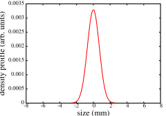
Figure 1: Charge density distribution along the $x$ axis.

We computed the electric field along the $x$ axis using the above direct gridless spectral solver with $15\times 15$ modes and the electric field from a second order finite difference solver with $129\times 129$ grid points. The results are shown in Fig. 2.

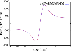
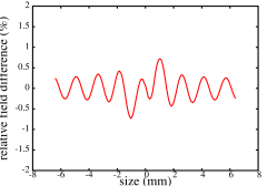
Figure 2: Electric field on $x$ axis from the above direct spectral solver (red) and from the 2nd order finite difference solver (green) (left), and the normalized relative field difference (right).

The solution of the spectral solver agrees with that of the finite difference solver very well with even $15\times 15$ modes due to the fast convergence property of the spectral method. The relative maximum field difference (normalized by the maximum field amplitude) between two solutions is below $2\%$. The use of the mode number in this example is somewhat empirical. It depends on the physical problem to be solved. If one knows about the smallest spatial structure of the problem, one can choose the mode number with the wavelength to resolve this spatial structure. Without knowing the detailed structure in the particle density distribution, one can use a trial-and-error method until the appropriate solution is attained.

Figure 3 shows the proton beam root-mean-square (rms) envelope evolution through $20$ FODO lattice periods.

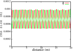
Figure 3: RMS envelope evolution of the beam.

The FODO lattice used in this example consists of two quadrupoles and three drifts in a single period. The total length of the period is $1$ meter. The zero current phase advance is about $87$ degrees and the phase advance with $100$ A current is about $74$ degrees. The relatively low intensity beam used in this example is to avoid space-charge driven resonance and to separate the numerical emittance growth from the physical emittance growth in the simulation.

The symplectic integrator is good for long term tracking since it helps preserve phase space structure during the numerical integration. Figure 4 shows the stroboscopic plots (every 10 periods) of $x-p_{x}$ and $y-p_{y}$ phase space evolution of a test particle through the last $20,000$ periods of the total $100,000$ lattice periods including the self-consistent space-charge forces. As a comparison, we also show in this figure the phase space evolution of the same initial test particle using the standard momentum conserved PIC method and the second order finite difference solver for space-charge calculation rob1 ; hockney .

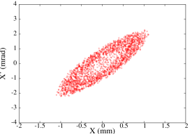
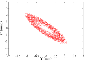
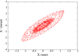
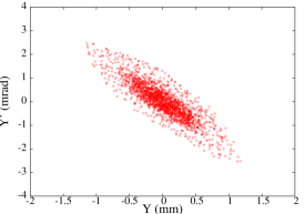
Figure 4: Stroboscopic plot (every 10 periods) of phase space evolution of a test particle from the symplectic-spectral model (top) and from the PIC-finite difference model (bottom).

Qualitatively, these two models show similar shapes in phase space. However, looking into the details of the phase space, they have quite different structures. The single particle phase space from the PIC model shows a dense core while the phase space from the symplectic multi-particle model shows a nearly hollow core. Figure 5 shows the 4-dimensional emittance growth ($\frac{\epsilon_{x}}{\epsilon_{x0}}\frac{\epsilon_{y}}{\epsilon_{y0}}-1$)% evolution from the symplectic model and that from the PIC model.

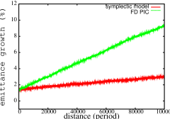
Figure 5: Four dimensional emittance growth evolution from the symplectic multi-particle spectral model (red) and from the PIC finite difference model(green).

It is seen that the symplectic model has a much smaller emittance growth than the PIC model. This emittance growth is a numerical artifact due to the small number of macroparticles ($50,000$) used in the simulation, which was studied in references noise1 ; noise2 ; noise3 . The small number of macroparticles introduces numerical errors in the computing of the electric potential and results in the artificial emittance growth. A more detailed study of the numerical emittance growth associated with this new method is under way and will be reported in future publication. The apparent non-zero emittance growth at the beginning is due to the charge redistribution of the initial Gaussian distribution within a much shorter time scale (not visible in the plot) compared with the total plotting time scale of $100,000$ periods.

IV Symplectic space-charge map for a 3D bunched beam

In a 3D bunched beam, the Hamiltonian $H_{2}$ can be written as rob2 :

$$H_{2} = \frac{\kappa\gamma_{0}}{2}\sum_{i=1}^{N_{p}}\sum_{j=1}^{N_{p}}\varphi({\bf r}_{i},{\bf r}_{j})$$ (35)

where $\kappa=q/(lmC^{2}\gamma_{0}^{2}\beta_{0})$, $l=C/\omega$ is the scaling length, and $\beta_{0}=v_{0}/C$. The above Hamiltonian includes both the electric potential and the longitudinal magnetic vector potential. The electric potential in the beam frame can be obtained from the solution of a three-dimensional Poisson’s equation:

$$\frac{\partial^{2}\phi}{\partial x^{2}}+\frac{\partial^{2}\phi}{\partial y^{2}}+\frac{\partial^{2}\phi}{\partial z^{2}}=-\frac{\rho}{\epsilon_{0}}$$ (36)

where $\rho$ is the charge density distribution in the beam frame. The boundary conditions for the electric potential inside the rectangular perfect conducting pipe are:

$$\phi(x=0,y,z) = 0$$ (37)

$$\phi(x=a,y,z) = 0$$ (38)

$$\phi(x,y=0,z) = 0$$ (39)

$$\phi(x,y=b,z) = 0$$ (40)

$$\phi(x,y,z=-\infty) = 0$$ (41)

$$\phi(x,y,z=\infty) = 0$$ (42)

where $a$ is the horizontal width of the pipe, $b$ is the vertical width of the pipe. The solution of the 3D Poisson equation subject to the above boundary conditions was studied with several numerical methods qiang1 ; qiang2 . To obtain a fast analytical solution of the electric potential we use an artificial boundary condition in this study. Here, the longitudinal open boundary condition is approximated by a finite domain Dirichlet boundary condition:

$$\phi(x,y,z=0) = 0$$ (43)

$$\phi(x,y,z=c) = 0$$ (44)

where $c$ is the length of the domain that is large enough so that the electric potential goes to zero at both ends of the domain. The choice of the length of the domain depends on how fast the electric potential vanishes outside the beam. From the reference qiang2 , we know that the solution of the electric potential for each transverse mode can be written as:

$$\phi^{lm}(z) = \frac{1}{2\gamma_{lm}\epsilon_{0}}\int_{-\infty}^{\infty}\exp(-\gamma_{lm}|z-z^{\prime}|)\rho^{lm}(z^{\prime})\ dz^{\prime}$$ (45)

where $\gamma^{2}_{lm}=(l\pi/a)^{2}+(m\pi/b)^{2}$. This solution decreases exponentially as a function of $z$ outside the beam. This suggests that a short distance (in the unit of aperture size) might be sufficient to have the electric potential approach to zero.

Given the boundary conditions in Eqs. 37-44, the electric potential $\phi$ and the source term $\rho$ can be approximated using three sine functions as:

$$\rho(x,y,z)=\sum_{l=1}^{N_{l}}\sum_{m=1}^{N_{m}}\sum_{n=1}^{N_{n}}\rho^{lmn}\sin(\alpha_{l}x)\sin(\beta_{m}y)\sin(\gamma_{n}z)$$ (46)

$$\phi(x,y,z)=\sum_{l=1}^{N_{l}}\sum_{m=1}^{N_{m}}\sum_{n=1}^{N_{n}}\phi^{lmn}\sin(\alpha_{l}x)\sin(\beta_{m}y)\sin(\gamma_{n}z)$$ (47)

where

$$\rho^{lmn}=\frac{8}{abc}\int_{0}^{a}\int_{0}^{b}\int_{0}^{c}\rho(x,y,z)\sin(\alpha_{l}x)\sin(\beta_{m}y)\sin(\gamma_{n}z)\ dxdydz$$ (48)

$$\phi^{lmn}=\frac{8}{abc}\int_{0}^{a}\int_{0}^{b}\int_{0}^{c}\phi(x,y,z)\sin(\alpha_{l}x)\sin(\beta_{m}y)\sin(\gamma_{n}z)\ dxdydz$$ (49)

where $\alpha_{l}=l\pi/a$, $\beta_{m}=m\pi/b$, $\gamma_{n}=n\pi/c$. Substituting the above expansions into the Poisson Eq. 36 and making use of the orthonormal condition of the sine functions, we obtain

$$\phi^{lmn} = \frac{\rho^{lmn}}{\epsilon_{0}\Gamma_{lmn}^{2}}$$ (50)

where $\Gamma_{lmn}^{2}=\alpha_{l}^{2}+\beta_{m}^{2}+\gamma_{n}^{2}$.

In the multi-particle tracking, the charge density $\rho(x,y,z)$ can be represented as:

$$\rho(x,y,z)=\sum_{j=1}^{N_{p}}w\delta(x-x_{j})\delta(y-y_{j})\delta(z-z_{j})$$ (51)

where $w$ is the charge weight of each individual particle and $\delta$ is the Dirac function. Using the above equation and Eq. 48 and Eq. 50, we obtain:

$$\phi^{lmn}=\frac{1}{\epsilon_{0}\Gamma_{lmn}^{2}}\frac{8}{abc}w\sum_{j=1}^{N_{p}}\sin(\alpha_{l}x_{j})\sin(\beta_{m}y_{j})\sin(\gamma_{n}z_{j})$$ (52)

and the electric potential as:

$$\phi(x,y,z)=\frac{1}{\epsilon_{0}}\frac{8}{abc}w\sum_{j=1}^{N_{p}}\sum_{l=1}^{N_{l}}\sum_{m=1}^{N_{m}}\sum_{n=1}^{N_{n}}\frac{1}{\Gamma_{lmn}^{2}}\sin(\alpha_{l}x_{j})\sin(\beta_{m}y_{j})\sin(\gamma_{n}z_{j})\sin(\alpha_{l}x)\sin(\beta_{m}y)\sin(\gamma_{n}z)$$ (53)

From the above electric potential, we obtain the interaction potential between particles $i$ and $j$ as:

$$\varphi(x_{i},y_{i},z_{i},x_{j},y_{j},z_{j})=\frac{1}{\epsilon_{0}}\frac{8}{abc}w\sum_{l=1}^{N_{l}}\sum_{m=1}^{N_{m}}\sum_{n=1}^{N_{n}}\frac{1}{\Gamma_{lmn}^{2}}\sin(\alpha_{l}x_{j})\sin(\beta_{m}y_{j})\sin(\gamma_{n}z_{j})\sin(\alpha_{l}x_{i})\sin(\beta_{m}y_{i})\sin(\gamma_{n}z_{i})$$ (54)

Given particle’s spatial coordinates $(x_{i},y_{i},\theta_{i})$ in the laboratory frame, the particle spatial coordinates in the beam frame $(x_{i},y_{i},z_{i})$ can be obtained under the following approximation:

$$z_{i} = -l\gamma_{0}\beta_{0}\theta_{i}$$ (55)

Now, the space-charge Hamiltonian $H_{2}$ can be written as:

$$H_{2}=\frac{1}{2\epsilon_{0}}\frac{8}{abc}w\kappa\gamma_{0}\sum_{i=1}^{N_{p}}\sum_{j=1}^{N_{p}}\sum_{l=1}^{N_{l}}\sum_{m=1}^{N_{m}}\sum_{n=1}^{N_{n}}\frac{1}{\Gamma_{lmn}^{2}}\sin(\alpha_{l}x_{j})\sin(\beta_{m}y_{j})\sin(-\gamma_{n}l\gamma_{0}\beta_{0}\theta_{j})\sin(\alpha_{l}x_{i})\sin(\beta_{m}y_{i})\sin(-\gamma_{n}l\gamma_{0}\beta_{0}\theta_{i})$$ (56)

The one-step symplectic transfer map ${\mathcal{M}}_{2}$ of the particle $i$ with this Hamiltonian is given as:

$$p_{xi}(\tau) = p_{xi}(0)-\tau\frac{1}{\epsilon_{0}}\frac{8}{abc}wl\kappa\gamma_{0}\sum_{j=1}^{N_{p}}\sum_{l=1}^{N_{l}}\sum_{m=1}^{N_{m}}\sum_{n=1}^{N_{n}}\frac{\alpha_{l}}{\Gamma_{lmn}^{2}}$$

$$\sin(\alpha_{l}x_{j})\sin(\beta_{m}y_{j})\sin(-\gamma_{n}l\gamma_{0}\beta_{0}\theta_{j})\cos(\alpha_{l}x_{i})\sin(\beta_{m}y_{i})\sin(-\gamma_{n}l\gamma_{0}\beta_{0}\theta_{i})$$

$$p_{yi}(\tau) = p_{yi}(0)-\tau\frac{1}{\epsilon_{0}}\frac{8}{abc}wl\kappa\gamma_{0}\sum_{j=1}^{N_{p}}\sum_{l=1}^{N_{l}}\sum_{m=1}^{N_{m}}\sum_{n=1}^{N_{n}}\frac{\beta_{m}}{\Gamma_{lmn}^{2}}$$

$$\sin(\alpha_{l}x_{j})\sin(\beta_{m}y_{j})\sin(-\gamma_{n}l\gamma_{0}\beta_{0}\theta_{j})\sin(\alpha_{l}x_{i})\cos(\beta_{m}y_{i})\sin(-\gamma_{n}l\gamma_{0}\beta_{0}\theta_{i})$$

$$p_{ti}(\tau) = p_{ti}(0)+\tau\frac{1}{\epsilon_{0}}\frac{8}{abc}wl\kappa\gamma_{0}^{2}\beta_{0}\sum_{j=1}^{N_{p}}\sum_{l=1}^{N_{l}}\sum_{m=1}^{N_{m}}\sum_{n=1}^{N_{n}}\frac{\gamma_{n}}{\Gamma_{lmn}^{2}}$$ (57)

$$\sin(\alpha_{l}x_{j})\sin(\beta_{m}y_{j})\sin(-\gamma_{n}l\gamma_{0}\beta_{0}\theta_{j})\sin(\alpha_{l}x_{i})\sin(\beta_{m}y_{i})\cos(-\gamma_{n}l\gamma_{0}\beta_{0}\theta_{i})$$

where both $p_{xi}$ and $p_{yi}$ are normalized by $mC$.

As an illustration of above symplectic model, we simulated a $1$ GeV, 3D bunched proton beam transporting through a periodic focusing channel. The initial transverse and longitudinal density profiles of the beam are shown in Fig. 6. The beam has a 3D Gaussian distribution with a longitudinal to transverse aspect ratio of three.

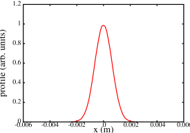
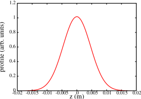
Figure 6: The transverse (left) and longitudinal (right) density profiles of a 3D bunched beam.

Figure 7 shows the relative transverse electric field difference along the x-axis and the longitudinal electric field difference along the z-axis using above gridless spectral method with $15\times 15\times 15$ modes and using a spectral-finite difference solver qiang1 with $129\times 129\times 257$ grid points.

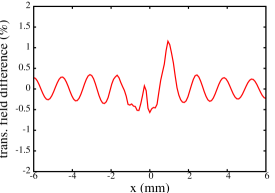
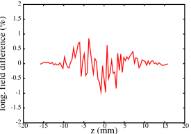
Figure 7: Relative transverse electric field difference along x-axis (left) and longitudinal electric field difference along z-axis (right) from the gridless spectral method and the spectral-finite difference solver.

It is seen that even with only $15$ modes in each direction, the gridless spectral solver produces space charge fields in good agreement with the fields from the spectral-finite difference solver with finer resolution. The relative maximum field differences (normalized by the maximum field amplitude along the axis) are below $2\%$ in both directions.

Figure 8 shows the transverse and the longitudinal rms envelope evolution through a periodic focusing channel. Each period of the focusing channel consists of two transverse uniform focusing elements, two longitudinal uniform focusing elements, and four drifts. The total length of the period is one meter. The zero current phase advance in a single period is about $86$ degrees in the transverse dimension and $40$ degrees in the longitudinal direction. The phase advance with $0.1$ A average current at $100$ MHz RF frequency is about $81$ degrees in the transverse direction and $39$ degrees in the longitudinal direction.

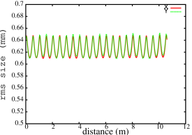
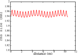
Figure 8: Transverse (left) and longitudinal (right) RMS envelope evolution of the bunched beam inside a periodic focusing channel.

Figure 9 shows the six-dimensional rms emittance growth ($\frac{\epsilon_{x}}{\epsilon_{x0}}\frac{\epsilon_{y}}{\epsilon_{y0}}\frac{\epsilon_{z}}{\epsilon_{z0}}-1$)% evolution through the periodic focusing channel from the above symplectic gridless spectral model and from the standard PIC method with the spectral-finite difference Poisson solver.

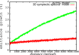
Figure 9: Six-dimensional rms emittance growth evolution in the periodic channel from the symplectic spectral model (red) and from the PIC (green).

It is seen that the symplectic spectral model gives much less numerical emittance growth than the standard PIC method in the simulation using $160,000$ macroparticles.

V computational complexity

The gridless symplectic multi-particle spectral model can be used for long-term tracking study including space-charge effects. The computational complexity of this model scales as $O(N_{mode}\times N_{p})$, where $N_{mode}$ is the total number of modes. The standard PIC model can have a computational cost of $O(N_{p})+O(N_{grid}logN_{grid})$ when an efficient Poisson solver is used, where $N_{grid}$ is the total number of grid points. This suggests that the PIC model would be faster than the symplectic multi-particle spectral model on a single processor computer. However, the symplectic multi-particle spectral model is very easy to be parallelized on multi-processor computer. One can distribute all macroparticles uniformly across processors to achieve a perfect load balance. By using a spectral method with exponentially decreasing errors, the number of modes $N_{mode}$ can be kept within a relatively small number, which significantly improves the computing speed. Figure 10 shows the parallel speedup of the symplectic multi-particle spectral model as a function of the number of processors for a fixed problem size, i.e. $\sim 50,000$ macroparticles and $15\times 15$ modes in the 2D model and $\sim 160,000$ macroparticles and $15\times 15\times 15$ modes in the 3D model. It is seen that the speedup increases almost linearly for both models. This is because both models have perfect load balance among all processors. The only communication involved in these models is a global reduction operation to obtain the density distribution in the frequency domain. The decrease of the speedup in the 2D case might be due to the specific computer architecture used in this timing study, which has $24$ shared memory computing cores inside a node. Outside the node, the communication among processors (cores) is slowed down due to the across node communication. The above scaling results show that the symplectic multi-particle spectral space-charge tracking model can have a good scalability on multi-processor parallel computers and is especially suitable for tracking simulations on large scale supercomputers or GPU computers.

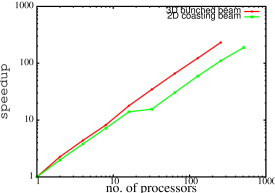
Figure 10: Parallel speedup of the 2D and the 3D symplectic tracking models on a Cray XC30 computer.

VI Conclusions

In this paper, we proposed a new symplectic multi-particle tracking model for self-consistent space-charge simulation. This model uses a gridless spectral method to calculate the space-charge potential and while avoiding the error associated with numerical grid in the standard PIC model. It also shows much less numerical noise driven emittance growth than the PIC method for long term simulation. Even though the computational cost of the symplectic spectral model is higher than the PIC method on a single processor computer, the proposed model scales well on multi-processor parallel computers. It has a perfect load balance and uniform data structure, which is suitable for GPU parallel implementation. The new symplectic multi-particle spectral model enables researchers to carry out long term tracking studies including space-charge effects.

The symplectic space-charge transfer map presented in this paper assumes a rectangular perfect conducting pipe. A transverse open boundary condition might be approximated using this model by moving the conducting wall away from the beam. For a general boundary condition, it is quite difficult to obtain an analytical expression of the electric potential from an arbitrary density distribution. For a round perfect conducting pipe, a Fourier mode and a Bessel mode might be used to approximate the particle density distribution and the electric potential of the Poisson equation in a cylindric coordinate system qiang1 . However, it takes more time to compute the Bessel function expansion than the simple sine function expansion.

The symplectic space-charge model presented here also assumes a straight conducting pipe. A study of the solution of the Poisson equation in a bended conducting pipe using the Frenet-Serret coordinate was done in reference qiang5 and shows that for a large normalized bending radius (bending radius/transverse aperture size), e.g. 100, there is barely any difference between the straight pipe solution and the bended pipe solution. This condition (large normalized bending radius) can be satisfied in most circular accelerators. Thus, the symplectic space-charge model in this paper can still be used for space-charge simulation in circular machines.

References

- (1) A. Friedman, D. P. Grote, and I. Haber, Phys. Fluids B 4 , 2203 (1992).
- (2) K. R. Crandall et al., LANL Technical Report No. LA-UR-96-1836, 1997.
- (3) H. Takeda and J. H. Billen, Recent developments of the accelerator design code PARMILA, in Proc. XIX International Linac Conference, Chicago, August 1998, p. 156.
- (4) J. Qiang, R. D. Ryne, S. Habib, V. Decyk, J. Comput. Phys. 163, 434, 2000.
- (5) P. N. Ostroumov and K. W. Shepard. Phys. Rev. ST. Accel. Beams 11, 030101 (2001).
- (6) R. Duperrier, Phys. Rev. ST Accel. Beams 3, 124201, 2000.
- (7) H. Qin, R. C. Davidson, W. W. Lee, and R. Kolesnikov, Nucl. Instr. Meth. in Phys. Res. A 464, 477 (2001).
- (8) J. Qiang, S. Lidia, R. D. Ryne, and C. Limborg-Deprey, Phys. Rev. ST Accel. Beams 9, 044204, 2006.
- (9) J. Amundson, P. Spentzouris, J. Qiang and R. Ryne, J. Comp. Phys. vol. 211, 229 (2006).
- (10) http://www.pulsar.nl/gpt/.
- (11) http://amas.web.psi.ch/docs/opal/opal_user_guide.pdf.
- (12) https://www.cockcroft.ac.uk/events/SpaceCharge15/index.html.
- (13) J. Xiao, J. Liu, H. Qin, and Z. Yu, Phys. Plasmas 20, 102517 (2013)
- (14) E. G. Evstatiev and B. A. Shadwick, J. Comput. Phys. 245, p.376 (2013).
- (15) B. A. Shadwick, A. B. Stamm, and E. G. Evstatiev, Phys. Plasmas 21, 055708 (2014).
- (16) H. Qin et al., Nuclear Fusion 56, 014001, (2016).
- (17) S. Webb, Plasma Phys. Control. Fusion 58, 034007, (2016).
- (18) E. Forest, “Beam Dynamics: A New Attitude and Framework,” The Physics and Technology of Particle and Photon Beams, Vol. 8 (Harwood Academic Publishers, Amsterdam, 1998).
- (19) R. D. Ryne, “Computational Methods in Accelerator Physics,” US Particle Accelerator class note, 2012.
- (20) A. J. Dragt, “Lie Methods for Nonlinear Dynamics with Applications to Accelerator Physics,” 2016.
- (21) E. Forest and R. D. Ruth, Physica D 43, p. 105, 1990.
- (22) H. Yoshida, Phys. Lett. A 150, p. 262, 1990.
- (23) http://mad.web.cern.ch/mad/.
- (24) E. Forest, J. Phys. A: Mathe Gen. 39 p. 5321, 2006.
- (25) D. Gottlieb and S. A. Orszag, Numerical Analysis of Spectral Methods: Theory and Applications, Society for Industrial and Applied Mathematics, 1977.
- (26) B. Fornberg, A Practical Guide to Pseudospectral Methods, Cambridge University Press, 1998.
- (27) J. Boyd, Chebyshev and Fourier Spectral Methods, Dover Publications, Inc. 2000.
- (28) J. Qiang and R. D. Ryne, Comp. Phys. Comm. 138, p. 18, 2001.
- (29) J. Qiang, Comp. Phys. Comm. 203, p. 122, 2016.
- (30) R.W. Hockney, J.W. Eastwood, Computer Simulation Using Particles, Adam Hilger, New York, 1988.
- (31) I. Hofmann and O. Boine-Frankenheim, Phys. Rev. ST Accel. Beams 17, 124201 (2014).
- (32) O. Boine-Frankenheim, I. Hofmann, J. Struckmeier, and S. Appel, Nucl. Instrum. Methods Phys. Res., Sect. A 770, 164 (2015).
- (33) F. Kesting and G. Franchetti, Phys. Rev. ST Accel. Beams 18, 114201 (2015).
- (34) R. D. Ryne, ”The Linear Map for an rf Gap Including Acceleration ,” LANL Report 836 R5 ST 2629 (1991).
- (35) J. Qiang and R. L. Gluckstern, Comp. Phys. Comm. 160, p. 120, 2004.