Ideal Relaxation of the Hopf Fibration

Abstract

Ideal MHD relaxation is the topology-conserving reconfiguration of a magnetic field into a lower energy state where the net force is zero. This is achieved by modeling the plasma as perfectly conducting viscous fluid. It is an important tool for investigating plasma equilibria and is often used to study the magnetic configurations in fusion devices and astrophysical plasmas. We study the equilibrium reached by a localized magnetic field through the topology conserving relaxation of a magnetic field based on the Hopf fibration in which magnetic field lines are closed circles that are all linked with one another. Magnetic fields with this topology have recently been shown to occur in non-ideal numerical simulations. Our results show that any localized field can only attain equilibrium if there is a finite external pressure, and that for such a field a Taylor state is unattainable. We find an equilibrium plasma configuration that is characterized by a lowered pressure in a toroidal region, with field lines lying on surfaces of constant pressure. Therefore, the field is in a Grad-Shafranov equilibrium. Localized helical magnetic fields are found when plasma is ejected from astrophysical bodies and subsequently relaxes against the background plasma, as well as on earth in plasmoids generated by e.g. a Marshall gun. This work shows under which conditions an equilibrium can be reached and identifies a toroidal depression as the characteristic feature of such a configuration.

I Introduction

A fundamental question in plasma physics is: Given a magnetic field configuration, what equilibrium state can it attain? This question was posed by Arnol’d Arnold (1974) who considered the static equilibria of ideal (zero magnetic diffusivity), incompressible magnetohydrodynamics (MHD), such that the magnetic topology remains unchanged. Subsequent work by Moffatt expanded this problem for various geometries and connected the equilibrium solutions to solutions of Euler equations for fluid flow (Moffatt, 1985). J.B. Taylor (Taylor, 1974) considered the problem for a different scenario; a plasma with a very low (but finite) resistivity in a toroidal device. His conjecture was both elegant and experimentally accurate: the field relaxes to a linear force-free state with the same helicity of the initial field. Taylor’s theory is an application of the work of Woltjer, who showed that a force-free (Beltrami) state is the lowest energy configuration that a field can attain under conservation of helicityWoltjer (1958a, b, 1959).

Due to the elegance and predictive power of Taylor’s conjecture, this principle of relaxation to a linear force-free state is often applied also in geometries beyond which it is strictly applicable. Recently there have been several papers addressing this, and identifying geometries in which the final state after relaxation is distinctly not a Taylor state. Simulations on magnetic field relaxation in a flux tube geometry have shown additional topological constraints associated with the field line connectivity that hinder relaxation to a force-free state Yeates et al. (2010). Also in one-dimensional resistive simulations fields were found not to converge to a linear force-free state Moffatt (2015). Furthermore, in our recent work we investigated the resistive decay of linked flux rings and tubes that converge to an MHD equilibrium that is not force-free Smiet et al. (2015).

The magnetic topology of this last example is remarkable, the field is localized, has finite energy, and field lines lie on nested toroidal surfaces such that on each surface the ratio of poloidal to toroidal winding is nearly identical. This last observation implies that the magnetic field topology is related to the mathematical structure called the Hopf map(Hopf, 1931). Fibers of this map form circles that are all linked with each other, and lie on nested toroidal surfaces. The structure of the Hopf map has been used in many branches of physics, amongst others, to describe structures in superfluids Volovik and Mineev (1977) and spinor Bose-Einstein condensates (Kawaguchi et al., 2008; Hall et al., 2016). It also forms the basis for new analytical solutions to Maxwell’s equations Rañada (1989); Irvine and Bouwmeester (2008) and Einstein’s equations Thompson et al. (2015). In ideal, incompressible MHD the Hopf map has been used to generate solutions of the ideal MHD equations called topological solitons (Kamchatnov, 1982; Sagdeev et al., 1986).

Even though the localized MHD equilibriumSmiet et al. (2015) has similar magnetic topology to the Hopf fibration, the geometry is different. The equilibrium consists of a balance between the pressure gradient force, directed inwards towards the magnetic axis, and the Lorentz force, directed outwards. In this paper we investigate exactly this equilibrium, and how it geometrically relates to fields derived from the Hopf map. We take fields with these well-defined magnetic topologies, and find their equilibrium configurations using a relaxation method that exactly conserves field line topology and converges to a static equilibrium which is a solution of the ideal MHD equations.

The choice for this initial topology is inspired by the numerical results on linked ringsSmiet et al. (2015), but there are many other works in which localized MHD equilibria are investigated and to which our results apply. Localized magnetic structures have been described in numerical relaxation experiments and are referred to as magnetic bubbles (Gruzinov, 2010; Braithwaite, 2010; Zrake and East, 2016). Also in fusion research structures are described as compact toroids or plasmoids, which consist of magnetic field lines lying on closed surfacesBostick (1956). Sometimes these structures are described as embedded in a guide field, but in isolation these fields are localized and show a similar magnetic topology (Armstrong et al., 1980; Perkins et al., 1988; Wright, 1990). Some models for magnetic clouds, regions of increased magnetic field observed in the solar windBurlaga (1991), consider the cloud as a localized magnetic excitation, either a current-ring Kumar and Rust (1996), or a flare-generated spheromakIvanov and Harshiladze (1985).

In ideal MHD magnetic helicity, or linking of magnetic field lines, is exactly conserved. Magnetic helicity is defined as

$$H_{\rm M}=\int\mbox{\boldmath$A$}{}\cdot\bm{B}\ \mathrm{d}^{3}x,$$ (1)

where $A$ is the vector potential and $\bm{B}=\mbox{\boldmath$\nabla$}{}\times\mbox{\boldmath$A$}{}$ the magnetic field. Woltjer was the first to realize that the value of this integral is conserved in ideal MHD (Woltjer, 1958a). It has recently been shown that any regular integral invariant under volume-preserving transformations is equivalent to the helicity(Enciso et al., 2016). Moffatt (Moffatt, 1969; Arnold, 1974) gave helicity a topological interpretation; helicity is a measure for the self- and inter-linking of magnetic field lines in a plasma. The conservation of magnetic linking can also be physically understood by the fact that in a perfectly conducting fluid the magnetic flux through a fluid element cannot change, and the magnetic field is transported by the fluid flow, a condition referred to as the frozen in condition (Alfvén, 1942; Batchelor, 1950; Priest and Forbes, 2000). As a consequence, in ideal MHD any linking or knottedness of magnetic field lines cannot be undone, and the magnetic topologyHornig and Schindler (1996) is conserved. Ideal MHD thus conserves not only total magnetic helicity but also the linking of every field line with every other field line.

Simulating non-resistive MHD numerically using a fixed Eulerian grid is a notoriously difficult problem due to numerical errors in Eulerian finite difference schemes Press et al. (2007). It is possible to circumvent this by using a Lagrangian relaxation scheme (Pontin et al., 2009) which dissipates fluid motion but perfectly preserves the frozen in condition. This was recently implemented using mimetic numerical operators in the numerical code GLEMuR(Candelaresi et al., 2014). In this paper we study the non-resistive relaxation of magnetic fields with the topology of the Hopf map using this recently developed code. Lagrangian methods were also recently implemented in a 2d dissipationless ideal MHD evolution scheme to study current singularities Zhou et al. (2014).

The virial theorem of MHD is a useful tool to investigate possible MHD equilibrium configurationsChandrasekhar (1961); Kulsrud (2005). This theorem relates the second derivative of the moment of inertia $I$ to integrals over the volume and boundary of a region in the plasma, and is usually stated as:

$$\frac{{\rm d}{}^{2}I}{{\rm d}{}t^{2}}=-\int\limits_{\partial V}\mathbf{T}\cdot\mbox{\boldmath$r$}{}\cdot{\rm d}{}\mbox{\boldmath$s$}{}+\int\limits_{V}\mbox{\rm Tr}(\mathbf{T})\ {\rm d}{}^{3}x.$$ (2)

Here $\mbox{\rm Tr}(\mathbf{T})$ denotes the trace of the strain tensor $\mathbf{T}=\mathbf{T}_{\mbox{\boldmath$u$}{}}+\mathbf{T}_{p}+\mathbf{T}_{\bm{B}}$. This tensor has a velocity component $\mathbf{T}_{\mbox{\boldmath$u$}{}}=\rho\mbox{\boldmath$u$}{}\mbox{\boldmath$u$}{}$, a pressure component $\mathbf{T}_{p}=\mathbf{I}p$ and a component due to the magnetic forces $\mathbf{T}_{\bm{B}}=\mathbf{I}B^{2}/2-\bm{B}\bm{B}$. Here $\rho$ denotes the fluid density, $u$ the velocity and $V$ the domain. $r$ is the position vector and $s$ indicates the surface normal of the surface of the region.

A consequence of the virial theorem is that for any static equilibrium to exist ($I$ to remain constant), the contribution of the bulk must be compensated by corresponding stresses on the boundary. The integral over the bulk can be written as $\int_{V}\left(\rho u^{2}+3p+B^{2}\right){\rm d}{}^{3}x$, which is always positive. Any reorganization of the bulk can change the magnitude of this contribution, but it will always be finite, which implies that without any stresses on the surface, a plasma will always expand ($I$ will increase). Therefore, one of the surface terms must integrate to a non-zero value for any equilibrium.

If we consider a localized magnetic field, such as the Hopf field, which has the same magnetic field topology as the localized equilibria described in previous numerical experimentsSmiet et al. (2015), then their magnetic field strength vanishes at sufficient distance, where we can put our boundary. This leaves two possible configurations through which an equilibrium can be reached. The first configuration has a finite pressure at the boundary. Any expansion in the bulk will create a low-pressure region, which will prevent the structure from expanding indefinitely. The second configuration has finite magnetic stresses at the boundary. This can be achieved by adding a constant guide field that prevents the field from expanding indefinitely through magnetic tension from the guide field. We note that the first configuration can never converge to a Taylor state, i.e. a localized magnetic field cannot relax to a force-free configuration.

II The Hopf Field

In 1931 Heinz Hopf (Hopf, 1931) discovered a curious property of maps from the hypersphere $S^{3}$ onto the sphere $S^{2}$, namely that the fibers of the maps (pre-images of points on $S^{2}$) are circles in $S^{3}$ that are all linked. This class of functions can be extended to a function from $\mathbb{R}^{3}$ to $\mathbb{C}$ from which a divergence-free vector field in $\mathbb{R}^{3}$ can be constructed such that the integral curves (field lines) lie tangent to the original fibers of the map (Sagdeev et al., 1986; Rañada, 1989; Kamchatnov, 1982). This construction is illustrated in Figure 1.

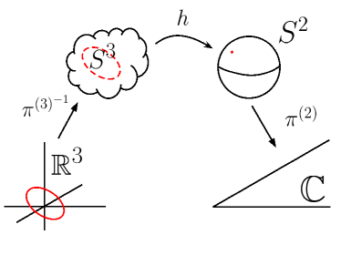
Figure 1: Illustration of the construction of a field with the topology of the Hopf map. The red dashed circle in $S^{3}$ is a fiber of the map. Through stereographic projection the fiber structure of the Hopf map is translated to $\mathbb{R}^{3}$ and a field that lies everywhere tangent to these circles is constructed.

The Hopf map can be modified as described in Arrayás and Trueba (2014), such that every fiber of the map lies on a toroidal surface with poloidal winding $\omega_{1}$ (short way around the torus) and toroidal winding $\omega_{2}$ (long way around the torus). If $\omega_{1}$ and $\omega_{2}$ are commensurable ($\omega_{1}/\omega_{2}\in\mathbb{Q}$), all field lines are $(\omega_{1}/{\rm gcd}(\omega_{1},\omega_{2}),\omega_{2}/{\rm gcd}(\omega_{1},\omega_{2}))$ torus knots where ${\rm gcd}(a,b)$ is the greatest common divisor of $a$ and $b$. From this map a field in $\mathbb{R}^{3}$ can be generated with that magnetic topology. Every field line lies on a torus and the tori form a nested set filling all of space. In this field there are two special field lines that do not form a $(\omega_{1},\omega_{2})$ torus knot. One lies on the largest torus, which reduces to a straight field line on the $z$-axis (torus through infinity), and the other field line lies on the degenerate (smallest) torus that reduces to a unit circle in the $xy$-plane and that is called the degenerate field line.

The vector field of this localized, finite-energy magnetic field with winding numbers $\omega_{1}$ and $\omega_{2}$ is given by:

$$\bm{B}_{\omega_{1},\omega_{2}}=\frac{4\sqrt{s}}{\pi(1+r^{2})^{3}\sqrt{\omega_{1}^{2}+\omega_{2}^{2}}}\begin{pmatrix}2(\omega_{2}y-\omega_{1}xz)\\ -2(\omega_{2}x+\omega_{1}yz)\\ \omega_{1}(-1+x^{2}+y^{2}-z^{2})\end{pmatrix},$$ (3)

with $r^{2}=x^{2}+y^{2}+z^{2}$ and $s$ is a scaling factor. The derivation of equation (3) is given in appendix A. Selected field lines for the $\bm{B}_{1,1}$ and $\bm{B}_{3,2}$ fields are shown in Figure 2.

In recent resistive numerical simulations Smiet et al. (2015) it was shown that magnetic fields consisting of initially linked field lines relax to an equilibrium where field lines lie on nested toroidal surfaces. The rotational transform (or $q$-factor) was seen to be within 10% constant for every magnetic surface in the structure. The field generated by equation (3) consists of field lines on nested toroidal surfaces with a constant rotational transform, which is determined by $\omega_{1}/\omega_{2}$, and thus is topologically similar to the fields observed in resistive simulation. Even though the fields have similar magnetic topology, the geometrical distribution of field is different. The magnetic field given by equation (3) is not in equilibrium, as there are large rotational Lorentz forces that cannot be balanced. Using a topology-conserving relaxation scheme we will see how these forces relax the magnetic field to a different geometry, but with the exact same magnetic topology.

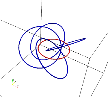
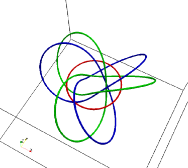
Figure 2: Several field lines of the initial magnetic field for the Hopf field with $\omega_{1}=\omega_{2}=1$ (upper panel) and the field with parameters $\omega_{1}=3$, $\omega_{2}=2$ (lower panel). We show select field lines with the ring at $||\bm{x}||=1,z=0$ (red) and two more field lines (blue and green). The upper field consists of linked magnetic flux rings, while the lower consists of linked trefoil knots.

The Lorentz force $\mbox{\boldmath$F$}{}_{\rm L}=\mbox{\boldmath$J$}{}\times\bm{B}$ can be decomposed as $\mbox{\boldmath$F$}{}_{\rm L}=\bm{B}\cdot\nabla\bm{B}-\nabla\bm{B}^{2}/2$, where $\bm{B}^{2}/2$ is referred to as magnetic pressure, and $\bm{B}\cdot\nabla\bm{B}$ is called magnetic tension. Magnetic pressure gives rise to a force pointing from regions with high magnetic field energy to regions of low magnetic energy. In the Hopf fibration magnetic energy is highly localized ($B_{1,1}^{2}=16/(\pi^{2}(1+r^{2})^{4})$), giving rise to a radial outward force. The magnetic tension force, on the other hand, is a force that resists the bending of magnetic field lines, and can effectively be seen as the result of tension in the field lines. Figure 7 shows how the magnetic tension and pressure interact to produce the Lorentz force in the Hopf field $\bm{B}_{1,1}$. In the $z=1$ plane the tension adds a clockwise twist to the field and a force toward the center, whereas the magnetic pressure points radially outward. The radial components largely cancel resulting in a predominantly rotational force around the $z$-axis. In the $z=0$ plane the forces only have a radial component, resulting in a net outwards force, and in the $z=-1$ plane the toroidal forces are opposite with respect to $z=1$.

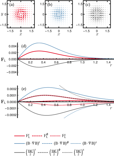
Figure 3: The Lorentz force and its components of magnetic pressure and magnetic tension for the Hopf field. (a-c) vector plots of the Lorentz force (red), magnetic tension (blue), and magnetic pressure force (grey) in the plane $z=1$. (d) Lorentz force and its components in the $z=0$ plane, where there is only a radial component. (e) Lorentz force and its components in the $z=-1$ plane. The $\phi$ and $\theta$ components of the magnetic tension force and the magnetic pressure force cancel each other to a large degree, leaving mainly the $\phi$ component. Because of the symmetry of the Hopf field, the components not shown in (a-c) can be read from (e).

II.1 Relation to the Kamchatnov-Hopf Soliton

The magnetic field in equation (3) was used by Kamchatnov (Kamchatnov, 1982) to describe an ideal MHD soliton, a solution to the ideal, incompressible MHD equations. By setting the fluid velocity equal to the (local) Alfvén speed,

$$\mbox{\boldmath$u$}{}_{\rm Kam}=\pm\frac{\bm{B}}{\sqrt{\rho}}$$ (4)

(a solution shown by Chandrasekhar to be stable (Chandrasekhar, 1956, 1961)) and using the pressure

$$p_{\rm Kam}=p_{\infty}-\frac{B^{2}}{2},$$ (5)

it follows from the ideal induction equation

$$\frac{\partial\bm{B}}{\partial t}=\mbox{\boldmath$\nabla$}{}\times(\mbox{\boldmath$u$}{}\times\bm{B}),$$ (6)

that the magnetic field is static. If we write the momentum equation as

$$\frac{\partial\mbox{\boldmath$u$}{}}{\partial t}+\mbox{\boldmath$u$}{}\cdot\nabla\mbox{\boldmath$u$}{}-\frac{1}{\rho}\bm{B}\cdot\nabla\bm{B}+\frac{1}{\rho}\nabla\left(p+\frac{B^{2}}{2}\right)=0,$$ (7)

and fill in the value for $\mbox{\boldmath$u$}{}_{\rm Kam}$ and $p_{\rm Kam}$ with $\bm{B}_{1,1}$ as a magnetic field this reduces to $\partial\mbox{\boldmath$u$}{}/\partial t=0$, a static configuration.

Kamchatnov’s construction solves the ideal, incompressible MHD equations, but this solution requires a fluid velocity parallel to the magnetic field at every point in space. Furthermore, it is necessary in Kamchatnov’s construction to include a confining pressure $p_{\infty}$. From the virial theorem we know that an external pressure can provide a restoring force so that a simpler equilibrium, without parallel fluid flow can be achieved. Furthermore, we need not restrict ourselves to the case of incompressible MHD, but we look for an equilibrium in the more general case of compressible barotropic ideal MHD. In our work we will consider the topology preserving, compressible relaxation of the magnetic field starting with the Hopf map. The field will relax to a different geometry but the topology preserving evolution will guarantee that the field remains topologically identical to the Hopf fibration.

III Methods

In order to simulate the topology conserving relaxation we restrict the field’s evolution to such that follow the ideal induction equation given in equation (6).

For the velocity field we use, depending on the case, two different approaches. In the magneto-frictional Chodura and Schlüter (1981) approach the velocity is proportional to the forces on the fluid element:

$$\mbox{\boldmath$u$}{}=\mbox{\boldmath$J$}{}\times\bm{B}-c_{\rm s}^{2}\mbox{\boldmath$\nabla$}{}\rho,$$ (8)

with the electric current density $\mbox{\boldmath$J$}{}=\mbox{\boldmath$\nabla$}{}\times\bm{B}$ and sound speed $c_{\rm s}$. The sound speed effectively determines the pressure in the simulation through $p=c_{\rm s}^{2}\rho$. It was shown by Craig and Sneyd (1986) that the magneto-frictional approach reduces the magnetic energy strictly monotonically. Alternatively, we can use an inertial evolution equation for the velocity (Candelaresi et al., 2015) with

$$\frac{{\rm d}{}\mbox{\boldmath$u$}{}}{{\rm d}{}t}=(\mbox{\boldmath$J$}{}\times\bm{B}-c_{\rm s}^{2}\mbox{\boldmath$\nabla$}{}\rho-\nu\mbox{\boldmath$u$}{})/\rho,$$ (9)

with the damping parameter $\nu$.

Numerical methods using fixed grids and finite differences typically introduce numerical dissipation which would effectively add the term $-\eta_{\rm num}\mbox{\boldmath$J$}{}$ on the right hand side of equation (6), with the numerical resistivity $\eta_{\rm num}$ over which there is little to no control. For every finite value of $\eta_{\rm num}$, however small, the field will invariably undergo a change in topology. To circumvent this we make use of a Lagrangian grid where the grid points move with the fluid (Craig and Sneyd, 1986; Candelaresi et al., 2014)

$$\frac{\partial\mbox{\boldmath$y$}{}(\bm{x},t)}{\partial\bm{x}}=\mbox{\boldmath$u$}{}(\mbox{\boldmath$y$}{}(\bm{x},t),t),$$ (10)

with the initial grid positions $\bm{x}$ and positions at later times $y$. The magnetic field on the distorted grid can be computed as the pull-back of a differential $2$-form, which then leads to the simple form (see for example references (Craig and Sneyd, 1986; Candelaresi et al., 2014)):

$$B_{i}(\bm{x},t)=\frac{1}{\Delta}\sum_{j=1}^{3}\frac{\partial y_{i}}{\partial x_{j}}B_{j}(\bm{x},0),$$ (11)

with $\Delta=\det{\left(\frac{\partial y_{i}}{\partial x_{j}}\right)}$.

We choose line tied boundary conditions where the velocity is set to zero and the normal component of the magnetic field is fixed. To compute the curl of the magnetic field $\mbox{\boldmath$J$}{}=\mbox{\boldmath$\nabla$}{}\times\bm{B}$ on the distorted grid we make use of mimetic spatial derivatives which increases accuracy and ensures $\mbox{\boldmath$\nabla$}{}\cdot\mbox{\boldmath$\nabla$}{}\times\bm{B}=0$ up to machine precision Hyman and Shashkov (1997, 1999).

It should be noted that equations (8) and (9) are both different from the momentum equation (7), and that therefore the evolution of the field is different from the evolution of a system adhering to the (dissipationless) ideal MHD equations. Nevertheless, it is clear that when the relaxation reaches a steady state, either by equation (8) or by (9), the field has reached a configuration in which all forces cancel. Our evolution equation also does not conserve energy, as any fluid motion is damped in order to expedite convergence to equilibrium. Since our main interest is investigating the existence and character of the equilibrium that is achieved under conservation of field line topology, the magneto-frictional and inertial evolution are both valid approaches to achieve this equilibrium. A different method which uses a Hamiltonian formulation for the field, and allows for relaxation under conservation of additional invariants, albeit under reduced dimensionality is found in Chikasue and Furukawa (2015).

Equations (8), (9), (10) and (11) are solved with the numerical code GLEMuR (Candelaresi et al., 2014; Candelaresi, 2015), written in CUDA and which runs on graphical processing units.

IV Topology Preserving Relaxation

We perform numerical experiments with the Hopf field as initial condition (eq. (3)) for different parameters $\omega_{1}$ and $\omega_{2}$, and the scaling factor $s$. The initial density is constant in space resulting in a constant pressure set by $c_{\rm s}^{2}$. All the simulations conserve the topology and obey either the magneto-frictional equation of motion (8) or the momentum equation (9).

IV.1 Field Expansion

We first analyze the relaxation of the $\bm{B}_{1,1}$ field with $s=2$. As can be expected from the distribution of forces in the initial field (Figure 7) the field expands outwards in the $xy$-plane, whilst the grid is twisted in opposite directions in the $z=1$ and $z=-1$ planes. The motion of the grid for the magneto-frictional runs with $c_{\rm s}^{2}=0.1$ are shown in supplemental videos 1 and 2 and in Figure 4 (Multimedia view). Supplemental video 1 shows the displacement of the grid initially in the $z=1$ plane, which twists in a clockwise direction. The colors indicate the vertical displacement of the grid, which moves towards the origin in the center, and upwards further out. If we look at the motion of the grid in the $y=0$ plane (supplemental video 2), we see the grid expanding outwards in the $z=0$ plane. The grid spacing increases around the $z=0,\ x=1$ location, resulting in the formation of a region of lowered pressure. As the field lines move with the grid, this is also the new location of the degenerate field line.

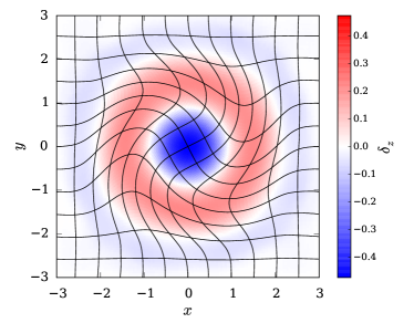
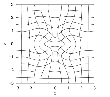
Figure 4: Grid distortion during relaxation to the final, relaxed configuration (approx. time $t=200$). (Upper panel): points initially in the $z=1$ plane (multimedia view), and (lower panel): distortion of the the $y=0$ plane (multimedia view). The color denotes the deviation of the grid points in the $z$-direction compared to $t=0$.

The expansion in the $xy$-plane can be tracked by measuring the change in radius $r$ of the degenerate field line. This is measured by the displacement of the point initially at $(1,0,0)$, and shown in Figure 5 (upper panel) for several different effective pressures. The effective pressure is set by the parameter $c_{\rm s}^{2}$, which enters into the equations as the proportionality factor between density $\rho$ and pressure $p$. For values lower than $c_{\rm s}^{2}=0.1$ the field expands to the computational boundaries. For higher values of $c_{\rm s}^{2}$ we see that, as expected, the expansion of the field levels off after a certain time, and the higher the confining pressure is, the less the configuration expands before it reaches equilibrium.

For $c_{\rm s}^{2}=0$ we expect an unconstrained expansion, while in the limit of $c_{\rm s}^{2}\to\infty$ we should see no expansion. Therefore, we plot the radius $r$ vs. $c_{\rm s}^{2}$ at time $t=100$ and fit the function

$$r=b(c_{\rm s}^{2})^{a}+1,$$ (12)

with fitting parameter $a=-0.160494$ and $b=0.16229561$. This fit gives a reasonable approximation for the expansion of the degenerate field line, indicating how the radius of the relaxed configuration depends on confining pressure. (Figure 5, lower panel).

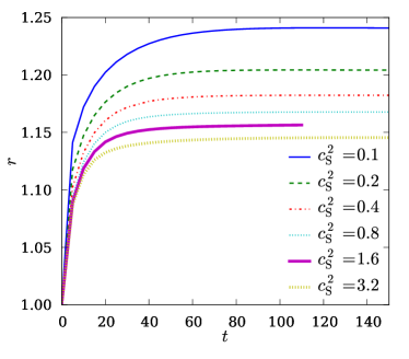
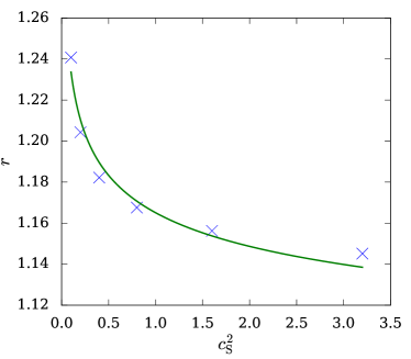
Figure 5: Time evolution of the degenerate field line in $\bm{B}_{1,1}$ at different effective pressures using the magneto-frictional approach (upper panel). Radii at time $t=150$ for different values of $c_{\rm s}^{2}$ with fit (lower panel).

During this expansion, the magnetic energy $B^{2}$ in the configuration sharply decreases due to the plasma expansion perpendicular to the magnetic field direction. This process can be seen in Figure 6, and it causes a drastic decrease in the magnetic pressure from the initial configuration.

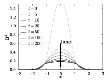
Figure 6: Squared of the magnetic field strength $B^{2}$ on the $x$-axis for different times for the $\bm{B}_{1,1}$ field. The field was relaxed using the magneto-frictional approach with $c_{\rm s}^{2}=0.2$. The magnetic field strength, and hence the magnetic pressure force, is greatly reduced during the relaxation by plasma expansion perpendicular to the field direction.

IV.2 Force Balance

Our simulations relax to a static configuration where the fluid velocity is zero. From the momentum equation (7), we can see that for any static equilibrium the pressure forces have to be balanced by a gradient in pressure:

$$\mbox{\boldmath$J$}{}\times\bm{B}=\mbox{\boldmath$\nabla$}{}p(=c_{\rm s}^{2}\mbox{\boldmath$\nabla$}{}\rho).$$ (13)

If we look at the relaxed field we see that the pressure is no longer constant, but the plasma has reorganized to create a toroidally-shaped region of lower pressure. The Lorentz force is also different in the relaxed configuration. The magnetic pressure contribution has been greatly reduced by the lowering of magnetic field strength accompanying the expansion, and the Lorentz force is now directed outwards, away from the degenerate field line. The condition of force balance in equation (13) is achieved in the simulation run, as can be seen in Figure 7. The Lorentz force $\mbox{\boldmath$J$}{}\times\bm{B}$ is balanced by the pressure force $-\nabla p=-c_{\rm s}^{2}\nabla\rho$, such that the total force is zero.

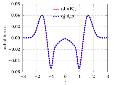
Figure 7: Radial component of the Lorentz force and radial component of the pressure gradient along the $x$-axis. The field was relaxed using the inertial approach with $c_{\rm s}^{2}=0.1$ and $\nu=1$. The two forces balance each other almost perfectly, indicating that an equilibrium is reached.

Another consequence of the equilibrium condition is that the pressure must be constant on magnetic field lines, and thus on the toroidal surfaces on which the field lines lie. By construction every field line in the Hopf field is a closed circle, but the circles lie on the surfaces of nested tori. These surfaces become visible if we consider the field with parameters $\omega_{1}=1$ and $\omega_{2}=1.01$, such that every field line is a $(100,101)$ torus knot. This field is locally nearly indistinguishable from the $\bm{B}_{1,1}$ field, but by tracing a single field line the toroidal surface on which the field line lies becomes visible. By plotting the intersections of such a field line with the $xz$-plane (constructing a Poincaré plot), we see a cross section of the magnetic surfaces. These magnetic surfaces are plotted together with the contours of constant pressure in the relaxed magnetic configuration in Figure 8. The contours of constant pressure clearly conform to the shape of the magnetic surfaces, especially near the degenerate field line. We attribute the discrepancy between the outermost magnetic surfaces and pressure surfaces to the fact that both the pressure gradient and/or the magnetic field strength are low at these locations, leading to a slow magneto-frictional convergence to equilibrium.

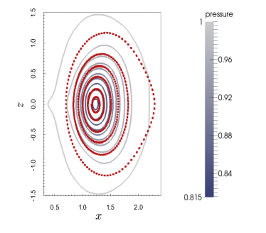
Figure 8: Magnetic surfaces (red squares) and pressure contours (colored lines) in the $xz$-plane for for the relaxed $\bm{B}_{1,1.01}$ field. The inner magnetic surfaces coincide with the pressure surfaces. Because the pressure gradients and Lorentz force are much lower on the outer surfaces, convergence to the equilibrium state is much slower.

Since the initial configuration is axisymmetric, and the resultant forces are as well, the configuration will remain axisymmetric through the entire evolution. The topology preserving relaxation method thus relaxes the magnetic field to an axisymmetric configuration where the magnetic forces are balanced by the pressure gradient. This kind of equilibrium can, in principle, be described by a solution to the Grad-Shafranov equation(Shafranov, 1966), but finding the exact functional form is a non-trivial task.

From the combination of the lowering of magnetic energy shown in Figure 6 and the lowering of the pressure in a toroidal region as seen in Figure 8 we understand how the equilibrium is achieved in light of the virial theorem. Recall from equation (2) that the volume contribution consists of three terms, $\rho u^{2}$, $3p$, and $B^{2}$. The contribution of the velocity is zero in equilibrium. As the field expands, the relative contribution of $B^{2}$ drops. The fluid that is expelled from the toroidal region causes a slight increase in pressure distributed over the entire surface. An equilibrium can be achieved when this negative contribution balances the reduced magnetic pressure of the distorted field.

The force-balanced equilibrium state obtained in these ideal relaxation experiments bears strong resemblance with quasi-stable magnetic structures found in various recent simulations, such as magnetic bubbles in(Gruzinov, 2010), freely decaying relativistic turbulence in(Zrake and East, 2016), and self-organizing knotted magnetic structures in(Smiet et al., 2015).

IV.3 Dependence on $\omega_{1}$ and $\omega_{2}$

To investigate the effects of different field line topologies we simulate the ideal relaxation of $\bm{B}_{3,2}$ and $\bm{B}_{2,3}$ with $c_{\rm s}^{2}=0.1$ and the scaling factor $s=1$. These two fields have exactly the same magnetic energy, but their magnetic topology, and the spatial distribution of magnetic pressure is different. In $\bm{B}_{3,2}$ the field lines make 3 poloidal (short way around the torus) windings for two toroidal windings. If we look at equation (3), we can see that $\omega_{1}$ (responsible for the poloidal winding) multiplies the $z$-component of the field, and increases the field strength along the $z$-axis of the configuration, whereas $\omega_{2}$ increases the magnetic pressure around the degenerate torus in the $xy$-plane.

When we relax the field we see that both choices of $\omega_{1}$ and $\omega_{2}$ yield an equilibrium, but the magnetic energy and pressure distributions are different, as can be seen in Figure 9. The radial expansion of the $\bm{B}_{3,2}$ simulation is much larger than that of $\bm{B}_{2,3}$, indicating that the degenerate torus (located at the minimum in pressure) is pushed further outwards. Note that the $\bm{B}_{3,2}$ equilibrium, which started out with relatively higher magnetic pressure on the $z$-axis, now shows highest field around the degenerate torus. The $\bm{B}_{2,3}$ field now has a highest magnetic field strength around the origin.

We can intuitively understand the behavior of these fields by recalling a well known observation in MHD; under internal forces a magnetic flux ring contracts and fattens, whilst a ring of current becomes thinner and stretches(Bellan, 2008). A ring of current gives rise to a magnetic field with only poloidal magnetic field lines, whereas a ring of magnetic flux consists of purely toroidal magnetic field lines. The fields we consider lie in between these two extreme configurations. The stronger the poloidal winding, the more the configuration resembles a current ring, and therefore this configuration will stretch relatively more. This will leave a relatively high magnetic field around the degenerate torus, as we can see in the equilibrium achieved by the $\bm{B}_{3,2}$ field. The $\bm{B}_{2,3}$ field has a relatively higher toroidal field, and will therefore expand less, leaving a high field around the $z$-axis.

Even though the exact distribution of magnetic energy and the magnetic field topology are different, the equilibrium is always characterized by a toroidal region of lowered pressure. All simulations start with constant hydrostatic pressure, and the observed final magnetic energy distribution is then given by the deformation that balances the dip in hydrostatic pressure with the lowered magnetic pressure. A different initial pressure distribution would also result in qualitatively different equilibrium magnetic energy distributions, but the essential features of the equilibrium would remain the same.

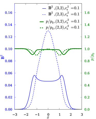
Figure 9: Magnetic energy density and normalized pressure on the $x$-axis for simulation runs with $c_{\rm s}^{2}=0.1$ and different ratio of poloidal to toroidal winding. The magnetic energy distribution is different in the two relaxed configurations, with the $\bm{B}_{3,2}$ simulation showing highest magnetic field strength around the degenerate torus, and the $\bm{B}_{2,3}$ configuration the highest field strength around the $z$-axis.

IV.4 Force-Balance with a mean magnetic field.

As noted in the introduction, it is possible to balance the field if the contribution of $\mathbf{T}_{\bm{B}}$ is non-zero at the boundary, i.e. the field is balanced by a finite external magnetic pressure. We investigate this by evolving $\bm{B}_{1,1}$ in a weak background field $\bm{B}_{\rm bck}=-0.02\mbox{\boldmath$e$}{}_{z}$ such that the final field is $\bm{B}=\bm{B}_{1,1}+\bm{B}_{\rm bck}$. It should be noted that this background field changes the magnetic topology of the initial condition. The new magnetic topology is such that field lines far away from the $z$-axis, where the field strength is opposite, but weaker than the guide field do not form magnetic surfaces, but extend from $z=-\infty$ to $z=\infty$. The same is the case for field lines close to the $z$-axis. On the magnetic surfaces that remain toroidal the ratio of poloidal to toroidal winding now changes from surface to surface.

For our numerical experiment we reduce the effective pressure by setting $c_{\rm s}^{2}=0.01$. This setting is much too low for the magnetic field to reach equilibrium within the simulation box without a guide field, but with the guide field an equilibrium is reached. The density and magnetic energy distribution are shown in Figure 10.

As the field expands, it pushes the guide field outwards, creating a restoring magnetic tension force. At the same time the magnetic field strength decreases, and the external magnetic pressure force halts the expansion. A finite, although very low, effective pressure is necessary to prevent the field from expanding indefinitely in the direction of the field lines. As we can see, the region of lowered pressure is much larger in the guide field simulation, which is to be expected from such a low value of $c_{\rm s}^{2}$. This numerical result suggests that in three dimensions a localized magnetic excitation can only achieve equilibrium if there is a finite external pressure. We note that this is in contrast to promising results found in two dimensional simulations (Zrake and East, 2016; Gruzinov, 2010), where localized magnetic excitations, called magnetic bubbles, are found in zero-pressure MHD and Force-Free Electrodynamics.

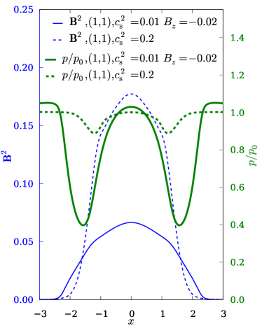
Figure 10: Magnetic energy density and normalized pressure on the $x$-axis for simulation runs with $1:1$ ratio of poloidal to toroidal winding with and without background magnetic field.

V Discussion and conclusions

We have shown how a localized magnetic excitation, in particular a Hopf field, relaxes to a configuration which is an equilibrium in an ideal, compressible plasma. The virial theorem implies that for any equilibrium to exist, there must either be a finite external pressure, or a guide field to attain equilibrium. The equilibrium that is achieved consists of a toroidal depression and is not a Taylor state.

We have used a topology preserving Lagrangian relaxation scheme that converges to an equilibrium configuration and observe the equilibrium in a wide range of parameters and different realizations of the Hopf map. In contrast to the topological solitons described by Kamchatnov(Kamchatnov, 1982), these configurations are static, and do not require a fluid velocity to balance the equations. These configurations are therefore static topological solitons in compressible MHD. The magnetic configurations remain axisymmetric under time evolution, and an equilibrium is achieved when magnetic field lines conform to the toroidal surfaces of constant pressure. The Lorentz force is balanced by the gradient in pressure and the obtained equilibria can be considered Grad Shafranov equilibria (Shafranov, 1966). Changing the magnetic topology of the initial field, by adjusting the ratio of toroidal to poloidal winding yields a qualitatively similar equilibrium, with a different distribution of magnetic energy.

Recent numerical simulations have shown that localized helical magnetic configurations can be generated in resistive plasma(Smiet et al., 2015; Gruzinov, 2010). The equilibrium we observe here is similar to what is observed in the resistive simulations, except that the ideal relaxation conserves field line topology, and therefore magnetic islands cannot be created.

Even though an equilibrium at zero pressure is impossible, any realistic plasma in which a topologically nontrivial field is embedded will have a (possibly very low) finite pressure. If such a field exists in a close to ideal plasma, the expansion will cause a decrease in magnetic field magnitude, and corresponding magnetic pressure. A finite external pressure, no matter how low, will give rise to an equilibrium at which the external magnetic pressure is able to confine the magnetic field in the manner described in this paper. Examples of where this could occur are in experiments with plasmoids Bostick (1956); Armstrong et al. (1980); Perkins et al. (1988); Wright (1990), and in astrophysical plasma such as the magnetic bubbles studied by BraithwaiteBraithwaite (2010).

It is interesting to contrast the equilibrium found in our simulations to the localized magnetic bubbles described in(Gruzinov, 2010; Zrake and East, 2016). The authors found a localized increase in pressure in two-dimensional relaxation at zero pressure, but as we have shown, such equilibria are impossible in three dimensions due to expansion along the guide field.

Localized three-dimensional magnetic excitations are possible, and the tell-tale signature of these relaxed states is a toroidal lowering of plasma pressure coinciding with the innermost magnetic surfaces. Such signatures could be detected in astrophysical observations, and help understanding the stability of magnetic fields in fusion plasmas.

Appendix A Derivation of the Hopf Field

If one considers the three-sphere $S^{3}$ embedded in $\mathbb{C}^{2}$ such that $S^{3}=\{(z_{1},z_{2})|z_{1}\bar{z}_{1}+z_{2}\bar{z}_{2}=1\}$, with $z_{1},z_{2}\in\mathbb{C}$ and one associates the complex plane with the sphere $S^{2}$ via stereographic projection $\pi^{(2)^{-1}}:\mathbb{C}\cup\infty\rightarrow S^{2}$, then a map from $S^{3}$ to $S^{2}$ can be given by the following expression:

$$h^{(\omega_{1},\omega_{2})}(z_{1},z_{2}):S^{3}\rightarrow S^{2}=\pi^{(2)^{-1}}\left({\frac{z_{1}^{(\omega_{2})}}{z_{2}^{(\omega_{1})}}}\right).$$ (14)

Here parenthesized exponentiation $z^{(\omega)}$ denotes the operation $z=re^{i\phi}\rightarrow re^{i\omega\theta}$ such that only the phase of the complex number is multiplied by $\omega$. If $\omega_{1}$ and $\omega_{2}$ are equal, this map reduces to Hopf map, where every fiber is a perfect circle and linked once with every other fiber. This is readily checked by observing that $h^{(1,1)}\left(z_{1},z_{2}\right)=h^{(1,1)}\left(z_{1}e^{i\theta},z_{2}e^{i\theta}\right)$, so the fibers of the map are indeed great circles in $S^{3}$. If $\omega_{1}$ and $\omega_{2}$ are not equal, but $\omega_{1}/\omega_{2}\in\mathbb{Q}$, the fibers are $(\omega_{1}/{\rm gcd}(\omega_{1},\omega_{2}),\omega_{2}/{\rm gcd}(\omega_{1},\omega_{2}))$ torus knots where ${\rm gcd}(a,b)$ is the greatest common divisor of $a$ and $b$.

In order to construct a field in $S^{3}$ from the Hopf map we modify the construction by Rañada Rañada (1989), using the method described in Arrayás and Trueba (2014) and Smiet et al. (2015) by extending the Hopf map to a complex-valued function from $S^{3}$ to $\mathbb{C}$:

$$\phi:\mathbb{R}^{3}\rightarrow\mathbb{C}=\pi^{(2)}\circ h^{(\omega_{1},\omega_{2})}\circ\pi^{(3)^{-1}},$$ (15)

where $\pi^{(3)^{-1}}$ denotes inverse stereographic projection from $S^{3}$ to $\mathbb{R}^{3}$.

The expression for the function $\phi$ becomes:

$$\phi=\frac{2(x+iy)^{(\omega_{2})}}{(2z+i(r^{2}-1))^{(\omega_{1})}},$$ (16)

where $r^{2}=x^{2}+y^{2}+z^{2}$. This construction is schematically illustrated in Figure 1. Since, by construction, $\phi$ is constant on linked curves in $\mathbb{R}^{3}$, the following expression results in a vector field that is everywhere tangent to the curves:

$$\tilde{\bm{B}}=\frac{1}{2\pi i}\frac{\nabla\phi\times\nabla\phi^{*}}{1+\phi\phi^{*}}.$$ (17)

This field is then given by

$$\tilde{\bm{B}}=\frac{4}{\pi(1+r^{2})^{3}}\begin{pmatrix}2(\omega_{2}y-\omega_{1}xz)\\ -2(\omega_{2}x+\omega_{1}yz)\\ \omega_{1}(-1+x^{2}+y^{2}-z^{2})\end{pmatrix}.$$ (18)

As a final step we normalize the magnetic field so the magnetic energy is independent of the choice of $\omega_{1}$ and $\omega_{2}$. Since

$$\int\tilde{\bm{B}}^{2}\ \mathrm{d}^{3}x=(\omega_{1}^{2}+\omega_{2}^{2}),$$ (19)

we divide equation (18) by $\sqrt{(\omega_{1}^{2}+\omega_{2}^{2})}$ to obtain equation (3) in the paper, safe the scaling factor $s$.

References

- Arnold (1974) V. I. Arnold, in Vladimir I. Arnold-Collected Works (Springer, 1974), pp. 357–375.
- Moffatt (1985) H. Moffatt, J. Fluid Mech. 159, 359 (1985).
- Taylor (1974) J. B. Taylor, Phys. Rev. Lett. 33, 1139 (1974).
- Woltjer (1958a) L. Woltjer, P. Natl. Acad. Sci. USA 44, 489 (1958a).
- Woltjer (1958b) L. Woltjer, P. Natl. Acad. Sci. USA 44, 833 (1958b).
- Woltjer (1959) L. Woltjer, P. Natl. Acad. Sci. USA 45, 769 (1959).
- Yeates et al. (2010) A. R. Yeates, G. Hornig, and A. L. Wilmot-Smith, Phys. Rev. Lett. 105, 085002 (2010).
- Moffatt (2015) H. Moffatt, J. Plasma Phys. 81, 905810608 (2015).
- Smiet et al. (2015) C. B. Smiet, S. Candelaresi, A. Thompson, J. Swearngin, J. W. Dalhuisen, and D. Bouwmeester, Phys. Rev. Lett. 115, 095001 (2015).
- Hopf (1931) H. Hopf, Math. Ann. 104, 637 (1931), ISSN 0025-5831.
- Volovik and Mineev (1977) G. E. Volovik and V. P. Mineev, Zh. Eksp. Teor. Fiz 73, 767 (1977).
- Kawaguchi et al. (2008) Y. Kawaguchi, M. Nitta, and M. Ueda, Phys. Rev. Lett. 100, 180403 (2008).
- Hall et al. (2016) D. S. Hall, M. W. Ray, K. Tiurev, E. Ruokokoski, A. H. Gheorghe, and M. Möttönen, Nature Physics (2016).
- Rañada (1989) A. F. Rañada, Lett. Math. Phys. 18, 97 (1989).
- Irvine and Bouwmeester (2008) W. T. M. Irvine and D. Bouwmeester, Nature Physics 4, 716 (2008).
- Thompson et al. (2015) A. Thompson, A. Wickes, J. Swearngin, and D. Bouwmeester, Journal of Physics A: Mathematical and Theoretical 48, 205202 (2015).
- Kamchatnov (1982) A. M. Kamchatnov, Soviet Journal of Experimental and Theoretical Physics 82, 117 (1982).
- Sagdeev et al. (1986) R. Z. Sagdeev, S. S. Moiseev, A. V. Tur, and V. V. Yanovskii, in Nonlinear phenomena in plasma physics and hydrodynamics (Mir Publishers, Moscow, 1986), vol. 1.
- Gruzinov (2010) A. Gruzinov, arXiv preprint arXiv:1006.1368 (2010).
- Braithwaite (2010) J. Braithwaite, Mon. Not. R. Astron. Soc. 406, 705 (2010).
- Zrake and East (2016) J. Zrake and W. E. East, Astrophys. J. 817, 89 (2016).
- Bostick (1956) W. H. Bostick, Physical Review 104, 292 (1956).
- Armstrong et al. (1980) W. T. Armstrong, D. Barnes, R. I. Bartsch, R. Commisso, C. Ekdahl, I. Henins, D. Hewett, H. Hoida, and T. Jarboe, in Proc. of the Eight International Conference on Plasma Physics and Controlled Nuclear Fusion Research, Brussels (1980).
- Perkins et al. (1988) L. Perkins, S. Ho, and J. Hammer, Nucl. Fusion 28, 1365 (1988).
- Wright (1990) B. Wright, Nucl. Fusion 30, 1739 (1990).
- Burlaga (1991) L. F. Burlaga, in Physics of the Inner Heliosphere II (Springer, 1991), pp. 1–22.
- Kumar and Rust (1996) A. Kumar and D. Rust, J. Geophys. Res. Space 101, 15667 (1996).
- Ivanov and Harshiladze (1985) K. Ivanov and A. Harshiladze, Sol. Phys. 98, 379 (1985).
- Enciso et al. (2016) A. Enciso, D. Peralta-Salas, and F. T. de Lizaur, P. Natl. Acad. Sci. USA 113, 2035 (2016).
- Moffatt (1969) H. K. Moffatt, J. Fluid Mech. 35, 117 (1969).
- Alfvén (1942) H. Alfvén, Nature 150, 405 (1942).
- Batchelor (1950) G. K. Batchelor, in Proceedings of the Royal Society of London A: Mathematical, Physical and Engineering Sciences (The Royal Society, 1950), vol. 201, pp. 405–416.
- Priest and Forbes (2000) E. R. Priest and T. G. Forbes, Magnetic reconnection: MHD theory and applications (Cambridge University Press, 2000).
- Hornig and Schindler (1996) G. Hornig and K. Schindler, Phys. Plasmas 3, 781 (1996).
- Press et al. (2007) W. H. Press, S. A. Teukolsky, W. T. Vetterling, and B. P. Flannery, Numerical Recipes 3rd Edition: The Art of Scientific Computing (Cambridge University Press, 2007), 3rd ed.
- Pontin et al. (2009) D. I. Pontin, G. Hornig, A. L. Wilmot-Smith, and I. J. D. Craig, Astrophys. J. 700, 1449 (2009).
- Candelaresi et al. (2014) S. Candelaresi, D. I. Pontin, and G. Hornig, SIAM J. Sci. Comput. 36, B952 (2014).
- Zhou et al. (2014) Y. Zhou, H. Qin, J. W. Burby, and A. Bhattacharjee, Phys. Plasmas 21, 102109 (2014).
- Chandrasekhar (1961) S. Chandrasekhar, Hydrodynamic and Hydromagnetic Stability (Courier Corporation, 1961).
- Kulsrud (2005) R. M. Kulsrud, Plasma physics for astrophysics, vol. 77 (Princeton University Press Princeton, 2005).
- Arrayás and Trueba (2014) M. Arrayás and J. L. Trueba, Journal of Physics A: Mathematical and Theoretical 48, 025203 (2014).
- Chandrasekhar (1956) S. Chandrasekhar, P. Natl. Acad. Sci. USA 42, 273 (1956).
- Chodura and Schlüter (1981) R. Chodura and A. Schlüter, J. Comput. Phys. 41, 68 (1981).
- Craig and Sneyd (1986) I. J. D. Craig and A. D. Sneyd, Astrophys. J. 311, 451 (1986).
- Candelaresi et al. (2015) S. Candelaresi, D. I. Pontin, and G. Hornig, Astrophys. J. 808, 134 (2015), eprint 1505.03043.
- Hyman and Shashkov (1997) J. M. Hyman and M. Shashkov, Computers & Mathematics with Applications 33, 81 (1997).
- Hyman and Shashkov (1999) J. M. Hyman and M. Shashkov, J. Comput. Phys. 151, 881 (1999).
- Chikasue and Furukawa (2015) Y. Chikasue and M. Furukawa, Phys. Plasmas 22, 022511 (2015).
- Candelaresi (2015) S. Candelaresi, Glemur, https://github.com/SimonCan/glemur (2015), URL https://github.com/SimonCan/glemur.
- Shafranov (1966) V. D. Shafranov, Reviews of Plasma Physics 2, 103 (1966).
- Bellan (2008) P. M. Bellan, Fundamentals of plasma physics (Cambridge University Press, 2008).