Dynamical Conductivity of Dirac Materials

Abstract

For graphene (a Dirac material) it has been theoretically predicted and experimentally observed that DC resistivity is proportional to $T^{4}$ when the temperature is much less than Bloch- Grüneisen ($\Theta_{BG}$) temperature and T linear in opposite case ($T>>\Theta_{BG}$). Going beyond the DC case, we investigate the dynamical conductivity in graphene using the powerful method of memory function formalism. In the DC (zero frequency regime) limit, we obtained the above mention behavior which was previously obtained using the Bloch-Boltzmann kinetic equation. In the finite frequency regime, we obtained several new results: (1) the generalized Drude scattering rate, in the zero temperature limit, shows $\omega^{4}$ behavior at low frequencies ($\omega<<k_{B}\Theta_{BG}/\hbar$) and saturates at higher frequencies. We also observed the Holstein Mechanism, however, with different power laws from that in the case of metals; (2) At higher frequencies, $\omega>>k_{B}\Theta_{BG}/\hbar$, and higher temperatures $T>>\Theta_{BG}$, we observed that the generalized Drude scattering rate is linear in temperature. In addition, several other results are also obtained. With the experimental advancement of this field, these results should be experimentally tested.

I Introduction

In the recent years, Dirac materials have attracted great attention due to their novel properties which originate from their linear energy dispersion and the presence of Dirac points or lines JC ; TOW . Graphene is a unique two dimensional Dirac material, consisting of a single atom thick layer of carbon atoms that are closely packed in honeycomb lattice structure due to their $sp^{2}$ hybridisation Geim ; Novoselov ; Zhang ; Allen . The electronic band structure of graphene exhibits the high symmetry momentum points as $\Gamma$, K, $K^{{}^{\prime}}$ and M. The points (K and $K^{{}^{\prime}}$) where the conduction and valence band touch upon each other are called the Dirac points (showing electronic energy dispersion $E_{k}=\pm|k|$). The electronic transport in graphene is governed by the relativistic Dirac equation with massless charge carriers (Fermion)Avouris ; Novoselov ; Zhang . The Fermi velocity of charge carriers in graphene is roughly $10^{6}ms^{-1}$. Pristine graphene has a minimum ballistic conductivity $\sigma_{min}=4e^{2}/h$Sarma .

Among many observable anomalous properties, DC resistivity is the unique one because it is the first to be measured but the last to be understood. The experimentally measured temperature dependent resistivity shows the linear in temperature behavior at high temperatures and $T^{4}$ in the Bloch- Grüneisen (BG) regime at low temperature ($T<<\Theta_{BG}$) Efetov . The Bloch- Grüneisen (BG) temperature is defined in the next section. Recent theoretical investigationsEM ; Kaasbjerg ; Hwang have been conducted on graphene by taking into account acoustic phonon limited scattering in the Bloch-Grüneisen (BG) regime. In ref. EM the author analytically solves the Bloch- Boltzmann equation for electron-acoustic phonon scattering, and it is shown that DC resistivity of graphene is proportional to $T^{4}$ in the low temperature regime ($T<<\Theta_{BG}$) and T-linear in the opposite regime. On similar lines, in ref. Kaasbjerg ; Hwang the studies of DC resistivity is done within the Boltzmann kinetic theory for the case of electron-acoustic phonon scattering and results agree with the previous investigations mentioned above Efetov .

The problem of DC transport in graphene is also treated using Kubo’s linear response theory by several groups Ziegler ; KZ ; Gusynin ; EGM ; Mishchenko ; Nomura ; Horng ; TMR ; Radchenko ; Falkovsky ; Mahan . They obtained the universal and nonuniversal observations of minimal conductivity in graphene at frequency $\omega\rightarrow 0$. In the presence of electric field, Gusynin and Sharapov Gusynin analytically obtained the expressions for both the diagonal and off-diagonal conductivities in graphene. It has been observed that these conductivities show the unusual behavior with frequency, chemical potential, and applied field caused by Dirac like spectrum of quasi-particles in this material.

We now briefly review some recent studies of electronic transport in graphene. Earlier, Radchenko et. al TMR have numerically computed the DC conductivity in short range and long range scattering regime for the case of charged impurities Li ; Yan . Further, the same authors Radchenko have studied the effect of charge carriers on the transport properties of graphene within both the Kubo linear response formalism and the Bolch- Boltzmann approach. The conductivity dependence on carrier density shows sublinear behavior within the semiclassical Boltzmann calculation. However, in contrast to it, the linear behavior is observed within the Kubo formalism.

Based on the result of Kubo method in the case of the spin-orbital coupling impurity scattering, Liu et. al Liu observed that the diagonal conductivity shows a insulating gap at Dirac point, while in opposite case when applying semiclassical Boltzmann approach, the prediction of insulating gap is failed. It is realized that the low energy transport can not be explained by Boltzmann theory which occurs from the spin orbit coupling scattering.

Several experimental groups have studied the conductivity measurement in different frequency regimes (visible, infrared, near infrared and ultraviolet) Novoselov ; WZ ; NMR ; LI ; T. Stauber ; Bolotin ; Heo ; Park . From experimental investigations, it has been observed that conductivity versus carrier density shows linear to sublinear behavior. Experimentally, Zhang et. al WZ obtained the AC conductivity $\sigma(\omega)$ in tetrahertz (THz) frequency range 0.2-1.2 THz. At present, $\sigma(\omega)\propto\omega^{4}$ is not observed.

However, theoretical investigations of dynamical conductivity due to electron-acoustic phonon scattering in graphene is lacking. In this paper, we present our results of the calculation of dynamical conductivity of graphene using the memory function formalism. The memory function formalism was pioneered by Mori and Zwanzig Mori ; Zwanzig . This is one of the most useful method known as, projection operator method. The basic idea of this method is to study the time correlation function systematically in the case of many body correlated systems. Götze and Wölfle GW put this method on a more useful footing by introducing their perturbative scheme and used that to solve the electrical conductivity in simple metals by taking into account different interactions. We use the Götze - Wölfle method to investigate the dynamical conductivity of graphene.

This paper is organized as follows. In section II, we will discuss the memory function formalism to calculate the dynamical conductivity in graphene. In section III, the results and discussion of dynamical conductivity due to electron-acoustic phonon scattering in graphene will be explained analytically and numerically. Finally, we will summarize our results and present our conclusions.

II Memory function Formalism

Our aim is to study the dynamical conductivity of a two dimensional (2D) Dirac material such as graphene using the Memory function formalism. Following the previous work GW ; Singh ; Kubo , we are going to use an alternative representation of conductivity from Kubo’s formalism i.e.

$$\sigma(z,T) = i\frac{\chi_{0}}{z-M(z,T)}.$$ (1)

Here M(z) is the memory function. $z=\omega+i\delta$ is the complex frequency and we have taken the limit $\delta\rightarrow 0$. $\chi_{0}$ represents the static limit of correlation function (i.e. $\chi_{0}=Ne/m$). First, we will calculate the memory function. The memory function can be expressed through the current-current correlation function:

$$\chi(z) = \langle\langle j_{1};j_{1}\rangle\rangle=i\int_{0}^{\infty}e^{izt}\langle[j_{1},j_{1}]\rangle dt.$$ (2)

Here inner $\left<......\right>$ describes canonical ensemble averages and outer $\left<......\right>$ represents Laplace transform of the expectation value of the same. It was shown in GW ; Singh ; Pankaj ; Das that the correlation function can be written as:

$$\chi(z)=\frac{\langle\langle C;C\rangle\rangle_{z=0}-\langle\langle C;C\rangle\rangle_{z}}{z^{2}}.$$ (3)

Where $C=[j_{1},H]$. H is the total Hamiltonian of the system. And the memory function can be written as GW ; Singh ; Pankaj ; Das ;

$$M(z,T)\simeq\frac{z\chi(z)}{\chi_{0}}.$$ (4)

Using the above relation, we obtain an approximate expression for the memory function

$$M(z,T)=\frac{\langle\langle C;C\rangle\rangle_{z=0}-\langle\langle C;C\rangle\rangle_{z}}{z\chi_{0}}.$$ (5)

Defining $\phi(z)=\langle\langle C;C\rangle\rangle_{z}$, the memory function can be written as,

$$M(z,T)=\frac{\left[\phi(0)-\phi(z)\right]}{(z\chi_{0})}.$$ (6)

In the present work, we consider a two dimensional dirac material having linear isotropic energy dispersion $(\epsilon_{k}=\hbar v_{f}|\vec{k}|)$, where $k$ is the momentum and $v_{f}$ is the Fermi velocity. Also in the whole analytical calculation we consider the system of units where $\hbar=1$ and $k_{B}=1$. Thus, to study the memory function for Dirac material with electron-phonon scattering Ziman , we write the following Hamiltonian,

$$H = H_{electrons}+H_{electron-phonon}$$ (7)

Here

$$H_{e^{-}} = \sum_{\mathbf{k}\sigma}\epsilon_{k}c^{\dagger}_{\mathbf{k}\sigma}c_{\mathbf{k}\sigma}$$ (8)

$$H_{e^{-}-ph} = \sum_{\mathbf{k},\,\mathbf{k^{\prime}},\sigma}\left[D(\mathbf{k}-\mathbf{k^{\prime}})c^{\dagger}_{\mathbf{k}\sigma}c_{\mathbf{k^{\prime}}\sigma}b_{\mathbf{k}-\mathbf{k^{\prime}}}+H.\,c.\right].$$ (9)

Here, $c^{\dagger}_{\mathbf{k}\sigma}(c_{\mathbf{k}\sigma})$ is the creation (annihilation) operator having spin $\sigma$ and momentum k. $b^{\dagger}_{\mathbf{k}-\mathbf{k^{\prime}}}(b_{\mathbf{k}-\mathbf{k^{\prime}}})$ is the phonon creation (annihilation) operator having phonon wave vector $q=\mathbf{k}-\mathbf{k^{\prime}}$. The coefficient $D(\mathbf{k}-\mathbf{k^{\prime}})$ in the electron phonon Hamiltonian is given by the expression for acoustic phonon’s EM ; Sarma i.e.

$$D(q) = -i\bigg{(}\frac{\hbar}{2\rho_{m}\omega_{q}}\bigg{)}^{1/2}\times D_{0}q\left[1-\bigg{(}\frac{q}{2k_{f}}\bigg{)}^{2}\right]^{1/2}$$ (10)

Here, $D_{0}$ is the deformation potential coupling constant for graphene, $\rho_{m}$ is surface mass density. The phonons are considered as longitudinal accoustic having a dispersion of the form $\omega_{q}=v_{s}q$. Here $v_{s}$ is the sound velocity, and q is the phonon momentum. In the present case, we have the condition EM $\frac{\hbar\omega_{q}}{k_{B}}\leq min(\Theta_{BG},\Theta_{D})$ with $\Theta_{D}$ is the Debye temperature, and $\Theta_{BG}=2(\frac{v_{s}}{v_{f}})\frac{\epsilon_{f}}{k_{B}}$ the Bloch Grüneisen temperature. $\epsilon_{f}$ is the Fermi energy. For our computation, we need to compute $C$ and the correlator $\langle\langle C;C\rangle\rangle_{z}$. For this, we use the expression for electrical current as $j=\Sigma_{k\sigma}v_{x}(k)c^{\dagger}_{\mathbf{k}\sigma}c_{\mathbf{k}\sigma}$, where $v_{x}(k)$ is the velocity of carriers with momentum $\mathbf{k}$ in the x- direction. Now from the electron-phonon interaction part of the Hamiltonian (Eqn.9) we get,

$$C=\sum_{k,k^{\prime}}[v_{x}(\mathbf{k})-v_{x}(\mathbf{k^{\prime}})][D(\mathbf{k}-\mathbf{k^{\prime}})c^{\dagger}_{\mathbf{k}\sigma}c_{\mathbf{k^{\prime}}\sigma}b_{\mathbf{k}-\mathbf{k^{\prime}}}-H.c.].$$ (11)

With this expression, two particle correlator $\phi(z)=\langle\langle C;C\rangle\rangle$ can be computed as follows,

$$\phi(z)=-\sum_{k,k^{\prime},\sigma}\sum_{p,p^{\prime}}[v_{x}(\mathbf{k})-v_{x}(\mathbf{k^{\prime}})][v_{x}(\mathbf{p})-v_{x}(\mathbf{p^{\prime}})]$$

$$D(\mathbf{k}-\mathbf{k^{\prime}})D^{\star}(\mathbf{p}-\mathbf{p^{\prime}})$$

$$\left\langle\left\langle c^{\dagger}_{\mathbf{k}\sigma}c_{\mathbf{k^{\prime}}\sigma}b_{\mathbf{k}-\mathbf{k^{\prime}}};b^{\dagger}_{\mathbf{p}-\mathbf{p^{\prime}}}c^{\dagger}_{\mathbf{p^{\prime}}}c_{\mathbf{p}}\right\rangle\right\rangle$$

$$-\sum_{k,k^{\prime},\sigma}\sum_{p,p^{\prime}}[v_{x}(\mathbf{k})-v_{x}(\mathbf{k^{\prime}})][v_{x}(\mathbf{p})-v_{x}(\mathbf{p^{\prime}})]$$

$$D^{\star}(\mathbf{k}-\mathbf{k^{\prime}})D(\mathbf{p}-\mathbf{p^{\prime}})$$

$$\left\langle\left\langle c^{\dagger}_{\mathbf{k^{\prime}}\sigma}c_{\mathbf{k}\sigma}b^{\dagger}_{\mathbf{k}-\mathbf{k^{\prime}}};b_{\mathbf{p}-\mathbf{p^{\prime}}}c^{\dagger}_{\mathbf{p}}c_{\mathbf{p^{\prime}}}\right\rangle\right\rangle.$$ (12)

Further, simplifications of the correlation function $\langle\langle c^{\dagger}_{\mathbf{k}\sigma}c_{\mathbf{k^{\prime}}\sigma}b_{\mathbf{k}-\mathbf{k^{\prime}}};b^{\dagger}_{\mathbf{p}-\mathbf{p^{\prime}}}c^{\dagger}_{\mathbf{p^{\prime}}}c_{\mathbf{p}}\rangle\rangle$ leads to Singh :

$$-\frac{1}{\epsilon_{k}-\epsilon_{k^{\prime}}-\omega_{k-k^{\prime}}+z}[f_{k}(1-f_{k^{\prime}})(1+n_{\omega_{k-k^{\prime}}})$$

$$-f_{k}^{\prime}(1-f_{k})n_{\omega_{k-k^{\prime}}}]\delta_{p,k}\delta_{p,k^{\prime}}.$$ (13)

Here $f_{k}=\langle c^{\dagger}_{\mathbf{k}}c_{\mathbf{k}}\rangle$, $f_{k}^{\prime}=\langle c^{\dagger}_{\mathbf{k^{\prime}}}c_{\mathbf{k^{\prime}}}\rangle$ are the Fermi-Dirac distribution functions and, $n_{\omega_{k-k^{\prime}}}=\langle b^{\dagger}_{\mathbf{k}-\mathbf{k^{\prime}}}b_{\mathbf{k}-\mathbf{k^{\prime}}}\rangle$ is the Bose-Einstein distribution function. Similarly the second factor of $\phi(z)$ can be simplified with the combine result

$$\phi(z)=\sum_{k,k^{\prime}}\left|D(\mathbf{k}-\mathbf{k^{\prime}})\right|^{2}[v_{x}(\mathbf{k})-v_{x}(\mathbf{k^{\prime}})]^{2}$$

$$\times[{f(1-f^{\prime})(1+n_{-}))-f^{\prime}(1-f)n_{-}}]$$

$$\times\left[\frac{1}{(\epsilon_{k}-\epsilon_{k^{\prime}}-\omega_{-}+z)}+\frac{1}{(\epsilon_{k}-\epsilon_{k^{\prime}}-\omega_{-}-z)}\right].$$ (14)

Here we have used the notation $f=f_{k}$; $f^{\prime}=f_{k}^{\prime}$; $n_{-}=n_{\omega_{k-k^{\prime}}}$; and $\omega_{-}=\omega_{k-k^{\prime}}$.

Using the above expression in Eqn.6, the imaginary part of the memory function can be written as,

$$ImM(\omega,T) = \frac{\pi}{\chi_{0}}\sum_{kk^{\prime}}\left|D(\mathbf{k}-\mathbf{k^{\prime}})\right|^{2}[v_{x}(\mathbf{k})-v_{x}(\mathbf{k^{\prime}})]^{2}$$ (15)

$$\times[(1-f)f^{\prime}n_{-}]$$

$$\times\Bigg{[}\frac{(e^{\beta\omega}-1)}{\omega}\delta(\epsilon_{k}-\epsilon_{k^{\prime}}-\omega_{-}+\omega)-$$

$$..(\rm terms\,with\,\omega\rightarrow-\omega)\Bigg{]}.$$

After simplification, the final memory function expression becomes

$$ImM(\omega,T) = M_{0}\int_{0}^{q_{BG}}dq\times\frac{q^{3}}{k_{f}}\sqrt{1-({q}/{2k_{f}})^{2}}$$ (16)

$$\times\frac{1}{e^{\beta\omega_{q}}-1}\times\Bigg{\{}(1-\frac{\omega_{q}}{\omega})\frac{e^{\beta\omega}-1}{(e^{\beta(\omega-\omega_{q})}-1)}$$

$$+(\rm terms\,with\,\omega\,\rightarrow-\omega)..\Bigg{\}}.$$

The details of the calculations are given in Appendix [A]. Here, $q_{BG}$ being the Bloch- Grüneisen momentum. As discussed in Appendix [A], in the graphene case, the the radius of Fermi circle is smaller as compare to Debye circle. In the scattering process, we need to consider those phonons whose wave vector is less than the Fermi wave vector. Therefore, the upper cut off values of q integral is to be $2k_{f}$. Further, to obtain the information from the above expression, we analysed it in special limiting cases that are discussed in the next section III. Consider first the zero frequency limit.

III Results And Discussion

Case-I: DC limit case (at zero frequency)
Consider $\omega\rightarrow 0$ then in the (Eqn.16), curly bracket term will become

$$\left\{(1-\frac{\omega_{q}}{\omega})\frac{e^{\beta\omega}-1}{(e^{\beta(\omega-\omega_{q})}-1)}+(\rm terms\,with\,\omega\,\rightarrow-\omega)..\right\}$$

$$\approx\frac{2\beta\omega_{q}}{1-e^{-\beta\omega_{q}}}$$ (17)

With this expression, the imaginary part of the memory function (Eqn.16) can be written as,

$$ImM(0) = 2M_{0}\int_{0}^{q_{BG}}dq\times\frac{q^{3}}{k_{f}}\sqrt{1-({q}/{2k_{f}})^{2}}$$ (18)

$$\times\frac{1}{e^{\beta\omega_{q}}-1}\times\frac{\beta\omega_{q}}{1-e^{-\beta\omega_{q}}}$$

Using $x=\beta\omega_{q}$ and $\beta v_{s}q_{BG}=\beta k_{B}{\Theta_{BG}}=\frac{\Theta_{BG}}{T}$ and $q_{BG}\approx 2k_{f}$, we obtain

$$ImM(0) = \frac{2M_{0}}{k_{f}\beta^{4}v_{s}^{4}}\int_{0}^{\beta v_{s}q_{BG}}dx\times\frac{{x^{4}}\sqrt{1-({x}/{2k_{f}\beta v_{s}})^{2}}}{(e^{x}-1)(1-e^{-x})}$$ (19)

$$= \frac{2M_{0}}{k_{f}}\left(\frac{T}{\Theta_{BG}}\right)^{4}{q^{4}_{BG}}$$

$$\times\int_{0}^{\frac{\Theta_{BG}}{T}}dx\frac{{x^{4}}\sqrt{1-({x}/{(\Theta_{BG}/T)})^{2}}}{(e^{x}-1)(1-e^{-x})}$$

$$= \frac{2M_{0}}{k_{f}}\left(\frac{T}{\Theta_{BG}}\right)^{4}{q^{4}_{BG}}\int_{0}^{z}\frac{{x^{4}}\sqrt{1-({x}/{z})^{2}}}{(e^{x}-1)(1-e^{-x})}dx$$

$$= \frac{2M_{0}}{k_{f}}\left(\frac{T}{\Theta_{BG}}\right)^{4}{q^{4}_{BG}}\times{\mathcal{J}}_{4}(z)$$

Here, we have the following functionEM :

$${\mathcal{J}}_{n}(z)=\int_{0}^{z}\frac{x^{n}\sqrt{1-(x/z)^{2}}}{(1-e^{-x})(e^{x}-1)}dx$$ (20)

The asymptotic limit of this function, for $n>0$ an integer, is given by ${\mathcal{J}}_{n}(\infty)=n!\zeta(n)$, with $\zeta(n)$ the Riemann Zeta function. In particular, for $n=4$, it has the values $\zeta(4)=\pi^{4}/90$ .
Subcase(1): for low temperature behavior $T<<\Theta_{BG}$, $z\rightarrow\infty$, ${\mathcal{J}}_{n}(\infty)=4!\zeta(4)$. Thus,

$$ImM(0) = \frac{2M_{0}}{k_{f}}\left(\frac{T}{\Theta_{BG}}\right)^{4}{q^{4}_{BG}}\times\frac{4!\pi^{4}}{90}$$

$$ImM(0) \propto T^{4}.$$ (21)

Subcase(2): for high temperature behavior $T>>\Theta_{BG}$, $z\rightarrow zero$. Then ${\mathcal{J}}_{4}(z)\approx\frac{\pi}{16}\times z^{3}$ (see Appendix B).

Therefore, we find that the imaginary part of memory function at high temperature becomes

$$ImM(0) = \frac{2M_{0}}{k_{f}}\left(\frac{T}{\Theta_{BG}}\right){q^{4}_{BG}}\times\frac{\pi}{16}$$

$$ImM(0) \propto T.$$ (22)

These results are in agreement with the existing theoretical and experimental data reported in literature Efetov ; EM ; Hwang ; Kaasbjerg .

Case-II: Finite frequency regime (at zero temperature)

In $T\rightarrow 0$ limit case, the ultralow behavior can be analyzed in Eqn.16 at all frequencies. Thus the expression in curly bracket leads to $\left(1-\frac{\omega_{q}}{\omega}\right)e^{\beta\omega_{q}}$ at $\omega>\omega_{q}$, and $\left(\frac{\omega_{q}}{\omega}-1\right)e^{\beta\omega}$ at $\omega<\omega_{q}$.

$$ImM(\omega) = M_{0}\int_{0}^{q_{BG}}dq\times\frac{q^{3}}{k_{f}}\sqrt{1-({q}/{2k_{f}})^{2}}$$ (23)

$$\times\frac{1}{e^{\beta\omega_{q}}-1}\Theta(\omega-\omega_{q})\left(1-\frac{\omega_{q}}{\omega}\right)e^{\beta\omega_{q}}$$

$$+M_{0}\int_{0}^{q_{BG}}dq\times\frac{q^{3}}{k_{f}}\sqrt{1-({q}/{2k_{f}})^{2}}$$

$$\times\frac{1}{e^{\beta\omega_{q}}-1}\Theta(\omega_{q}-\omega)\left(\frac{\omega_{q}}{\omega}-1\right)e^{\beta\omega}.$$

$$ImM(\omega) = M_{0}\int_{0}^{\omega}d\omega_{q}\times\frac{{\omega_{q}}^{3}}{k_{f}v_{s}^{4}}\sqrt{1-({\omega_{q}}/{2k_{f}v_{s}})^{2}}$$ (24)

$$\times\frac{e^{\beta\omega_{q}}}{e^{\beta\omega_{q}}-1}\bigg{(}1-\frac{\omega_{q}}{\omega}\bigg{)}$$

$$+ M_{0}\int_{\omega}^{\omega_{BG}}d\omega_{q}\times\frac{{\omega_{q}}^{3}}{k_{f}v_{s}^{4}}\sqrt{1-({\omega_{q}}/{2k_{f}v_{s}})^{2}}$$

$$\times\frac{e^{\beta\omega}}{e^{\beta\omega_{q}}-1}\bigg{(}\frac{\omega_{q}}{\omega}-1\bigg{)}.$$

Here we consider $\omega_{BG}=2v_{s}k_{f}$ and $x^{\prime}=\omega_{q}$, then rewrite the above equation as:

$$ImM(\omega) = \frac{2M_{0}}{v_{s}^{3}}\int_{0}^{\omega}dx^{\prime}\times\frac{{x^{\prime}}^{3}}{\omega_{BG}}\sqrt{1-({x^{\prime}}/{\omega_{BG}})^{2}}$$ (25)

$$\times\frac{e^{\beta x^{\prime}}}{e^{\beta x^{\prime}}-1}\bigg{(}1-\frac{x^{\prime}}{\omega}\bigg{)}$$

$$+ \frac{2M_{0}}{v_{s}^{3}}\int_{\omega}^{\omega_{BG}}dx^{\prime}\times\frac{{x^{\prime}}^{3}}{\omega_{BG}}\sqrt{1-({x^{\prime}}/{\omega_{BG}})^{2}}$$

$$\times\frac{e^{\beta\omega}}{e^{\beta x^{\prime}}-1}\bigg{(}\frac{x^{\prime}}{\omega}-1\bigg{)}.$$

At $T\rightarrow 0$, the first term of Eqn.25 provides the dominating contribution (because second term is exponentially small). Thus, the imaginary part of the memory function becomes

$$ImM(\omega) = \frac{2M_{0}}{v_{s}^{3}}\int_{0}^{\omega}dx^{\prime}\times\frac{{x^{\prime}}^{3}}{\omega_{BG}}\sqrt{1-({x^{\prime}}/{\omega_{BG}})^{2}}\bigg{(}1-\frac{x^{\prime}}{\omega}\bigg{)}$$

Let $x^{\prime}/\omega_{BG}=y$, thus we have

$$ImM(\omega) = \frac{2M_{0}\omega_{BG}^{3}}{v_{s}^{3}}\Bigg{[}\int_{0}^{\frac{\omega}{\omega_{BG}}}dy\times y^{3}\sqrt{1-y^{2}}-$$ (27)

$$\frac{\omega_{BG}}{\omega}\int_{0}^{\frac{\omega}{\omega_{BG}}}dy\times y^{4}\sqrt{1-y^{2}})\Bigg{]}$$

At $\omega<<\omega_{BG}$, On solving the integral, we obtain

$$ImM(\omega) = \frac{M_{0}\omega^{4}}{10v_{s}^{3}\omega_{BG}}$$

$$ImM(\omega) \propto \omega^{4}.$$ (28)

Thus $\omega^{4}$ dependence of scattering rate is obtained in given Dirac material case. However, in metals, it shows the $\omega^{5}$ dependence.

In the case $\omega>>\omega_{BG}$, $T\rightarrow 0$, the imaginary part of the memory function is

$$ImM(\omega) = \frac{2M_{0}}{v_{s}^{3}}\int_{0}^{\omega_{BG}}dx^{\prime}\times\frac{{x^{\prime}}^{3}}{\omega_{BG}}\sqrt{1-({x^{\prime}}/{\omega_{BG}})^{2}}$$ (29)

$$\times\frac{e^{\beta x^{\prime}}}{e^{\beta x^{\prime}}-1}\bigg{(}1-\frac{x^{\prime}}{\omega}\bigg{)}$$

Again let $x^{\prime}/\omega_{BG}=y$, thus we have

$$ImM(\omega) = \frac{2M_{0}\omega_{BG}^{3}}{v_{s}^{3}}\Bigg{[}\int_{0}^{1}dy\times y^{3}\sqrt{1-y^{2}}-$$ (30)

$$\frac{\omega_{BG}}{\omega}\int_{0}^{1}dy\times y^{4}\sqrt{1-y^{2}})\Bigg{]}$$

On solving the integral in the above limits, we obtain,

$$ImM(\omega) = \frac{M_{0}\omega_{BG}^{3}}{v_{s}^{3}}\Bigg{[}\frac{4}{15}-\left(\frac{\omega_{BG}}{\omega}\right)\frac{\pi}{16}\Bigg{]}$$

$$ImM(\omega) = \Bigg{[}a-\frac{b}{\omega}\Bigg{]}.$$ (31)

Here, $a=\frac{4}{15}\frac{M_{0}\omega_{BG}^{3}}{v_{s}^{3}}$ and $b=\frac{\pi M_{0}\omega_{BG}^{4}}{16v_{s}^{3}}$. Thus in the high frequency limit it saturates.

Case-III: Finite frequency regime (at finite temperature)

Consider $\omega>>\Theta_{BG},T$ then in Eqn.16, curly bracket term can be simplified as

$$\left\{(1-\frac{\omega_{q}}{\omega})\frac{e^{\beta\omega}-1}{(e^{\beta(\omega-\omega_{q})}-1)}+(\rm terms\,with\,\omega\,\rightarrow-\omega)..\right\}$$

$$\approx 2(e^{\beta\omega_{q}}+1)$$ (32)

In this case the Eqn.16 becomes

$$ImM(\omega,T) = \frac{2M_{0}}{k_{f}}\int_{0}^{q_{BG}}q^{3}\sqrt{1-\left(\frac{q}{2k_{f}}\right)^{2}}\frac{(e^{\beta\omega_{q}}+1)}{(e^{\beta\omega_{q}}-1)}dq$$

$$= \frac{2M_{0}}{k_{f}}\int_{0}^{q_{BG}}q^{3}\sqrt{1-\left(\frac{q}{2k_{f}}\right)^{2}}\coth\bigg{(}{\frac{\beta\omega_{q}}{2}}\bigg{)}dq$$

Using $x=\beta\omega_{q}$ and $\beta v_{s}q_{BG}=\beta k_{B}{\Theta_{BG}}=\frac{\Theta_{BG}}{T}$.

$$ImM(\omega,T) = \frac{2M_{0}}{k_{f}}\left(\frac{T}{\Theta_{BG}}\right)^{4}{q_{BG}^{4}}\times\int_{0}^{\frac{\Theta_{BG}}{T}}dx\times{x^{3}}$$ (34)

$$\times\sqrt{1-({x}/{(\Theta_{BG}/T)})^{2}}\times\coth\left({\frac{x}{2}}\right)$$

$$= \frac{2M_{0}}{k_{f}}\left(\frac{T}{\Theta_{BG}}\right)^{4}{q_{BG}^{4}}\times J_{3}\left(\frac{\Theta_{BG}}{T}\right).$$

Here $J_{3}(z)=\int_{0}^{z}dx\times{x^{3}}\sqrt{1-({x}/{z})^{2}}\times\coth\left({\frac{x}{2}}\right)$.

In the low temperature case: $T<<\Theta_{BG}$, $z\rightarrow\infty$, $J_{3}(z)=\frac{z^{4}}{4}$ the resulting Eqn.34 is

$$ImM(\omega,T) = \frac{M_{0}}{2k_{f}}{q_{BG}^{4}}$$

$$ImM(\omega,T) \propto constant.$$ (35)

In the high temperature case: $T>>\Theta_{BG}$, $z\rightarrow\ 0$, $J_{3}(z)=\frac{\pi z^{3}}{8}$ the resulting Eqn.34 is

$$ImM(\omega,T) = \frac{\pi M_{0}}{4k_{f}}{q_{BG}^{4}}\left(\frac{T}{\Theta_{BG}}\right)$$

$$ImM(\omega,T) \propto T.$$ (36)

Hence the scattering rate is linearly dependent on temperature in high temperature case when $T>>\Theta_{BG}$ and $\omega>>\Theta_{BG},T$. All the above mentioned results in different limiting cases are given in the table 1.

$\omega$ and $T$ regime	$ImM(\omega)$
$\omega=0;\,\,\,\,T<<\Theta_{BG}$	$T^{4}.$
$\omega=0;\,\,\,\,T>>\Theta_{BG}$	$T$.
$\omega<<\omega_{BG};\,\,\,\,T\rightarrow 0$	$\omega^{4}$.
$\omega>>\omega_{BG};\,\,\,\,T\rightarrow 0$	$[a-\frac{b}{\omega}]$.
$\omega>>\Theta_{BG},T;\,\,\,\,T<<\Theta_{BG}$	$\propto constant.$
$\omega>>\Theta_{BG},T;\,\,\,\,T>>\Theta_{BG}$	$\propto T.$

Table 1: The results of imaginary part of the memory function in different limiting cases.

In the general case, we need to perform the integral in Eqn.16 numerically. With $\hbar=6.582\times 10^{-16}eV.s$ and Boltzmann constant $k_{B}=8.617\times 10^{-5}eV/K$, we perform the integral by setting frequency in energy units (in eV). Now we present our numerical results.

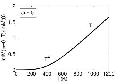
Figure 1: Variation of the imaginary part of the memory function with temperature at zero frequency.

In Fig.1, we show the variation of the imaginary part of the scaled memory function with temperature at zero frequency (ImM(0)=$\frac{N^{2}D_{0}^{2}}{32\pi^{3}\chi_{0}\rho_{m}v_{s}}$). From Fig.1, we observe that ImM(0, T) shows $T^{4}$ behavior at very low temperatures ($T<<\Theta_{BG}$) and T-linear behavior at high temperatures ($T>>\Theta_{BG}$). These features are in agreement with experimental data Efetov . In Fig.2, we depict the variation of $ImM(\omega,T)$ as a function of temperature at different frequencies. It shows that on increasing the frequency, scattering rate ($ImM(\omega)$) shifts upward. It is also observed that scattering rate shows linear behavior at high temperature, while at low temperature it shows saturation. We notice that even at zero temperature there is finite scattering. This is nothing but the Holstein mechanism for the present case.

The frequency dependent behavior of imaginary part of memory function at zero temperature is shown in Figure 3. From Fig.3, we observed that in the low frequency limit ($\hbar\omega<<k_{B}\Theta_{BG}$), $ImM(\omega,0)/ImM(0)$ shows $\omega^{4}$ behavior. While, at high frequency limit it becomes constant. In Fig.4, we depict the variation of imaginary part of memory function with frequency at various temperatures. It is observed that the $ImM(\omega,T)/ImM(0)$ increases with the increase in temperature at lower frequency regime while at the higher frequencies, it shows saturation behavior.

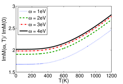
Figure 2: Variation of the imaginary part of the memory function with temperature at different frequencies.

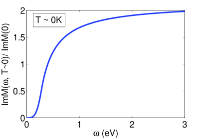
Figure 3: Variation of the imaginary part of the memory function with frequency at zero temperature for graphene.

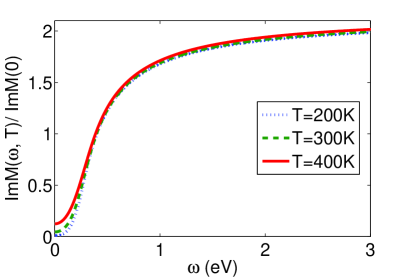
Figure 4: Variation of the imaginary part of the memory function with frequency at different temperatures.

IV Conclusions

We have presented a theoretical study of dynamical conductivity of a Dirac material by using the memory function formalism with electron- acoustic phonon scattering. We have reproduced the zero frequency (DC) results namely, $T^{4}$ behavior of resistivity at low temperature and T-linear at high temperature Efetov ; EM ; Sarma ; Kaasbjerg .

The Holstein mechanism TH which is the finite absorption of electromagnetic energy at zero temperature is also predicted by our calculations in 2D Dirac materials. However with different scaling behavior (Table 1). In the Holstein mechanism a photon generates an electron-hole pair along with the emission of a phonon (i.e. phonon assisted scattering). We predict that the scattering increases as $\omega^{4}$ in low temperature limit (refer to Table 1).

Both at high frequencies and at high temperatures $(T>>\Theta_{BG})$, we have observed the linear behavior of memory function with temperature, while at low temperature scattering rate $(ImM(\omega,T))$ becomes constant. These temperature and frequency dependent results should be experimentally tested.

Appendix A Derivation of Eqn.16

In the present study, we consider graphene (as a Dirac material), having linear isotropic energy dispersion $(\epsilon_{f}=v_{f}|\vec{k}|)$. To simplify equation (15), we insert $[v_{x}(\mathbf{k})-v_{x}(\mathbf{k^{\prime}})]^{2}=v_{f}^{2}(1-cos{\theta})$ and convert the sums into integrals in Eqn.15. We further reduced it by considering that $k$ is pointing along the $x$-direction and $k^{\prime}$ subtends an angle $\theta$ with it. Also we insert an integrated delta function$(1=\int dq\delta(q-|\mathbf{k}-\mathbf{k^{\prime}}|))$ over $q$ and resulting expression is

$$ImM(\omega) = \frac{\pi N^{2}v_{f}^{2}}{(2\pi)^{4}\chi_{0}}\int_{0}^{\infty}dqD_{q}^{2}\int_{0}^{\infty}{kdk}\int_{0}^{\infty}{k^{\prime}dk^{\prime}}$$ (37)

$$\int_{0}^{2\pi}d\theta(1-cos{\theta})\delta(q-\left|\mathbf{k}-\mathbf{k^{\prime}}\right|)$$

$$\times[(1-f)f^{\prime}n_{-}]$$

$$\times\Bigg{[}\frac{(e^{\beta\omega}-1)}{\omega}\delta(\epsilon_{k}-\epsilon_{k^{\prime}}-\omega_{-}+\omega)-$$

$$..(\rm terms\,with\,\omega\,\rightarrow-\omega)\Bigg{]}.$$

Shift the integration variables to $\epsilon_{k}=v_{f}k$, $\epsilon_{k}^{\prime}=v_{f}k^{\prime}$, $d\epsilon=v_{f}dk$. And for our convenience, we use the notation $\epsilon_{k}=\epsilon$ and $\epsilon_{k}^{\prime}=\epsilon^{\prime}$.

$$\Rightarrow\int_{0}^{\infty}{kdk}\int_{0}^{\infty}{k^{\prime}dk^{\prime}}=\frac{1}{v_{f}^{4}}\int_{0}^{\infty}{\epsilon d\epsilon}\int_{0}^{\infty}{\epsilon^{\prime}d\epsilon^{\prime}}$$

$$\delta(q-\left|\mathbf{k}-\mathbf{k^{\prime}}\right|)=\delta(q-\sqrt{k^{2}+k^{\prime 2}-2kk^{\prime}\cos\theta})$$ (38)

$$ImM(\omega) = \frac{\pi N^{2}}{(2\pi)^{4}\chi_{0}v_{f}^{2}}\int_{0}^{\infty}dqD_{q}^{2}\int_{0}^{\infty}{\epsilon d\epsilon}\int_{0}^{\infty}{\epsilon^{\prime}d\epsilon^{\prime}}$$ (39)

$$\int_{0}^{2\pi}d\theta(1-cos{\theta})\delta(q-\frac{1}{v_{f}}\sqrt{\epsilon^{2}+\epsilon^{\prime 2}-2\epsilon\epsilon^{\prime}\cos\theta})$$

$$\times[(1-f)f^{\prime}n_{-}]$$

$$\times\bigg{[}\frac{(e^{\beta\omega}-1)}{\omega}\delta(\epsilon-\epsilon^{\prime}-\omega_{-}+\omega)-...$$

$$(\rm terms\,with\,\omega\,\rightarrow-\omega)...\bigg{]}$$

Where, $\theta$ is the scattering angle. We are considering a degenerate system, and the magnitude of Fermi energy is much greater than $k_{B}T$. Thus, in graphene, electron-acoustic phonon scattering occurs in a very thin layer close to the Fermi surface. Within this $\epsilon\approx\epsilon^{\prime}\approx\epsilon_{f}$, the integral over $\theta$ can be simplified as follows:

$$I_{\theta} = \int_{0}^{2\pi}d\theta(1-cos{\theta})\delta(q-\frac{1}{v_{f}}\sqrt{\epsilon^{2}+\epsilon^{\prime 2}-2\epsilon\epsilon^{\prime}\cos\theta})$$ (40)

$$= \int_{0}^{2\pi}d\theta(1-cos{\theta})\delta(q-k_{f}\sqrt{2(1-\cos\theta)})$$

$$= \int_{0}^{\pi}d\theta(1-cos{\theta})\delta(q-k_{f}\sqrt{2(1-\cos\theta)})$$

$$+ \int_{\pi}^{2\pi}d\theta(1-cos{\theta})\delta(q-k_{f}\sqrt{2(1-\cos\theta)})$$

Here change to $x=1-cos{\theta}$

$$I_{\theta} = \int_{0}^{2}dx\frac{x}{\sqrt{2x-x^{2}}}\delta(q-k_{f}\sqrt{2x})$$ (41)

$$- \int_{2}^{0}dx\frac{x}{\sqrt{2x-x^{2}}}\delta(q-k_{f}\sqrt{2x})$$

$$= 2\int_{0}^{2}dx\frac{x}{\sqrt{2x-x^{2}}}\delta(q-k_{f}\sqrt{2x})$$

$$= 2\int_{0}^{2k_{f}}dt\frac{t^{3}}{2k_{f}^{4}}\frac{1}{\sqrt{\frac{t^{2}}{k_{f}^{2}}(1-\frac{t^{2}}{4k_{f}^{2}})}}\delta(q-t)$$

$$= 2\frac{q^{2}}{2k_{f}^{3}}\frac{1}{\sqrt{(1-\frac{q^{2}}{4k_{f}^{2}})}}=\frac{q^{2}}{k_{f}^{3}}\frac{1}{\sqrt{(1-\frac{q^{2}}{4k_{f}^{2}})}}$$

Substituting this value the $\theta$-integral into the memory function approximation. Thus the imaginary part of the memory function can be written as

$$ImM(\omega) = \frac{\pi N^{2}}{(2\pi)^{4}\chi_{0}}\int_{0}^{\infty}{d\epsilon}\int_{0}^{\infty}{d\epsilon^{\prime}}\int_{0}^{\infty}dq\times D_{q}^{2}\times\frac{q^{2}}{k_{f}}$$ (42)

$$\times\frac{1}{\sqrt{(1-\frac{q^{2}}{4k_{f}^{2}})}}\times\frac{1}{(e^{\beta\epsilon}+1)}\frac{1}{(e^{\beta\epsilon^{\prime}}+1)}$$

$$\times\frac{1}{(e^{\beta\omega_{q}}-1)}\Bigg{[}\frac{(e^{\beta\omega}-1)}{\omega}\delta(\epsilon-\epsilon^{\prime}-\omega_{-}+\omega)-$$

$$(\rm terms\,with\,\omega\,\rightarrow-\omega)..\Bigg{]}$$

Now performing the $\epsilon^{\prime}$ integral using the property of the delta functions. The resulting memory function expression becomes,

$$ImM(\omega) = \frac{\pi N^{2}}{(2\pi)^{4}\chi_{0}}\int_{0}^{\infty}{d\epsilon}\int_{0}^{\infty}dqD_{q}^{2}\times\frac{q^{2}}{k_{f}}\frac{1}{\sqrt{(1-\frac{q^{2}}{4k_{f}^{2}})}}$$ (43)

$$\times\frac{1}{e^{\beta\epsilon}+1}\frac{1}{e^{\beta\omega_{q}}-1}$$

$$\times\Bigg{[}\frac{(e^{\beta\omega}-1)}{\omega}\times\frac{1}{e^{\beta\epsilon}{e^{\beta(\omega-\omega_{q})}}+1}$$

$$-..(\rm terms\,with\,\omega\,\rightarrow-\omega)..\Bigg{]}.$$

And, then solving the integration over $\epsilon$ using the elementary method $\int_{-\infty}^{+\infty}dx\frac{e^{x}}{e^{x}+1}\frac{1}{e^{x+a}+1}$. The integral becomes

$$I_{\epsilon} = \int_{0}^{\infty}{d\epsilon}\frac{e^{\beta\epsilon}}{e^{\beta\epsilon}+1}\frac{1}{e^{\beta\epsilon+\beta(\omega-\omega_{q})}+1}$$ (44)

$$= \frac{(\omega-\omega_{q})}{e^{\beta(\omega-\omega_{q})}-1}$$

And thus the imaginary part of memory function is

$$ImM(\omega) = \frac{\pi N^{2}}{(2\pi)^{4}\chi_{0}}\int_{0}^{q_{BG}}dq\times D_{q}^{2}\times\frac{q^{2}}{k_{f}}\frac{1}{\sqrt{(1-\frac{q^{2}}{4k_{f}^{2}})}}$$ (45)

$$\times\frac{1}{e^{\beta\omega_{q}}-1}\times\Bigg{\{}\frac{(e^{\beta\omega}-1)}{\omega}\frac{(\omega-\omega_{q})}{e^{\beta(\omega-\omega_{q})}-1}$$

$$+(\rm terms\,with\,\omega\,\rightarrow-\omega)\Bigg{\}}$$

Using the relation $D_{q}$ from Eqn.10, defining $M_{0}=\frac{N^{2}D_{0}^{2}}{32\pi^{3}\chi_{0}\rho_{m}v_{s}}$, and $\omega_{q}=v_{s}q$, we have

$$ImM(\omega) = M_{0}\int_{0}^{q_{BG}}dq\times\frac{q^{3}}{k_{f}}\sqrt{1-({q}/{2k_{f}})^{2}}\frac{1}{e^{\beta\omega_{q}}-1}$$ (46)

$$\times\Bigg{\{}(1-\frac{\omega_{q}}{\omega})\frac{e^{\beta\omega}-1}{(e^{\beta(\omega-\omega_{q})}-1)}+$$

$$(\rm terms\,with\,\omega\,\rightarrow-\omega)..\Bigg{\}}.$$

Appendix B Some useful relations

We have used the following relation:

$${\mathcal{J}}_{n} = \int_{0}^{z}\frac{x^{4}\sqrt{1-(x/z)^{2}}}{(1-e^{-x})(e^{x}-1)}dx$$ (47)

For small z case, let $x=z\cos(\theta)$ then above integral becomes

$${\mathcal{J}}_{n} = \int_{0}^{\pi/2}\frac{z^{5}\cos^{4}(\theta)\sin^{2}(\theta)e^{z\cos(\theta)}}{(e^{z\cos(\theta)}-1)^{2}}d\theta$$ (48)

$$\approx \frac{\pi z^{3}}{16}$$

References

• (1) J. Cayssol, C. R. Physique 14, 760–778 (2013).
• (2) T. O. Wehling, A. M. Black-Schaffer, and A. V. Balatsky, Advances in Physics, Vol. 63, 1 (2014).
• (3) K. S. Novoselov, A. K. Geim, S. V. Morozov, D. Jiang, Y. Zhang, S. V. Dubonos, I. V. Grigorieva, A. A. Firsov, Science 306, 666 (2004).
• (4) K. S. Novoselov, A. K. Geim, S. V. Morozov, D. Jiang, M. I. Katsnelson, I. V. Grigorieva, S. V. Dubonos, and A. A. Firsov, Nature 438, 197 (2005).
• (5) Y. Zhang, Y.-W. Tan, H. L. Stormer, and P. Kim, Nature 438, 201 (2005).
• (6) M. J. Allen, V. C. Tung, and R. B. Kaner, Chem. Rev. 110, 132 (2010).
• (7) P. Avouris, Z. Chen, and V. Perebeinos, Nature Nanotechnology 2, 605 (2007).
• (8) S. D. Sarma, S. Adam, E. H. Hwang, and E. Rossi, Rev.Mod. Phys. 83, 407(2011).
• (9) D. K. Efetov and P. Kim, Phys. Rev. Lett. 105, 256805 (2010).
• (10) E. MuΓ±oz, J. Phys.: Condens. Matter 24, 195302 (2012).
• (11) E. H. Hwang and S. D. Sarma, Phys. Rev. B 77, 115449 (2008).
• (12) K. Kaasbjerg, K. S. Thygesen, and K. W. Jacobsen, Phys. Rev. B 85, 165440 (2012).
• (13) K. Ziegler, Phys. Rev. Lett. 97, 266802 (2006).
• (14) K. Ziegler, Phys. Rev. B 75, 233407 (2007).
• (15) V. P. Gusynin and S. G. Sharapov, Phys. Rev. B 73, 245411 (2006).
• (16) E. G. Mishchenko, Eur. Phys. Lett. 83, 17005 (2008).
• (17) E. G. Mishchenko, Phys. Rev. Lett. 103, 246802 (2009).
• (18) K. Nomura and A. H. MacDonald, Phys. Rev. Lett. 98, 076602 (2007).
• (19) L. A. Falkovsky and A.A. Varlamov, Eur. Phys. J. B 56, 281 (2007).
• (20) J. Horng, C-F Chen, B. Geng, C.r Girit, Y. Zhang, Z. Hao, H. A. Bechtel, M. Martin, A. Zettl, M. F. Crommie, Y. R. Shen, and F. Wang, Phys. Rev. B 83, 165113 (2011).
• (21) T. M. Radchenko, A. A. Shylau, and I. V. Zozoulenko, Phys. Rev. B 86, 035418 (2012).
• (22) T. M. Radchenko, A. A. Shylau, and I. V. Zozoulenko, Phys. Rev. B 87, 195448 (2013).
• (23) G. D. Mahan, Many-Particle Physics (Physics of Solids and Liquids), Kluwer Academic/Plenum Publishers (2000).
• (24) Q. Li, E. H. Hwang, E. Rossi, and S. Das Sarma,Phys. Rev. Lett.107, 156601 (2011).
• (25) J. Yan and M. S. Fuhrer, Phys. Rev. Lett.107, 206601 (2011).
• (26) Z. Liu, L. Jiang, and Y. Zheng, Scientific Reports 6, 23762 (2016).
• (27) N.M.R. Peres , T. Stauber, and A. H. Castro Neto, Euro. Phys. Lett. 84, 38002 (2008).
• (28) Z. Q. Li, E. A. Henriksen, Z. Jiang, Z. Hao, M. C. Martin,P. Kim, H. L. Stormer and D. N. Basov, Nature Phys. Lett. 4, 532 (2008).
• (29) T. Stauber, N.M.R. Peres, and A. K. Geim, Phys. Rev. B 78, 085432 (2008).
• (30) K. I. Bolotin, K. J. Sikes, J. Hone, H. L. Stormer, and P. Kim, Phys. Rev. Lett. 101, 096802 (2008).
• (31) J. Heo, H. J. Chung, S.-H Lee, H. Yang, D. H. Seo, J. K. Shin, U-In Chung, S. Seo, E. H. Hwang, and S. D. Sarma, Phys. Rev. B 84, 035421 (2011).
• (32) W. Zhang,P. H. Q. Pham, E. R. Browna and P. J. Burkeb, Nanoscale 6, 13895 (2014).
• (33) C-H Park, N. Bonini, T. Sohier, and G. Samsonidze, Nano Lett. 14, 1113 (2014).
• (34) R. Zwanzig, Phys. Rev. 124, 983 (1961).
• (35) H. Mori, Progr. Theor. Phys. 33, 423 (1965).
• (36) W. GΓΆtze and P. WΓΆlfle, Phys. Rev. B 6, 1226 (1972).
• (37) R. Kubo, J. Phys. Soc. Japan 12, 570 (1957).
• (38) N. Singh, Electronic Transport Theories: From Weakly to Strongly Correlated Materials, (Taylor and Francis Group, CRC Press) (2016).
• (39) N. Das and N. Singh, ArXiv e-prints,arXiv:1509.03418 (2015).
• (40) P. Bhalla, N. Das, and N. Singh, Phys. Lett. A, 380, 2000 (2016).
• (41) J. M. Ziman, Electrons and Phonons: The Theory of Transport Phenomena in Solids (Oxford Classic Texts in the Physical Sciences) (2001).
• (42) T. Holstein, Ann. Phys. 29, 410 (1964).