\setcopyright

acmcopyright \isbn978-1-4503-4590-3/17/04\acmPrice$15.00 http://dx.doi.org/10.1145/3049797.3049818

Forward Stochastic Reachability Analysis for Uncontrolled Linear Systems using Fourier Transforms

Abraham P. Vinod


Baisravan HomChaudhuri


Meeko M. K. Oishi


Electrical & Comp. Eng. University of New Mexico Albuquerque, NM 87131, USA aby.vinod@gmail.com Electrical & Comp. Eng. University of New Mexico Albuquerque, NM 87131, USA baisravan.hc@gmail.com Electrical & Comp. Eng. University of New Mexico Albuquerque, NM 87131, USA oishi@unm.edu
(2017)
Abstract

We propose a scalable method for forward stochastic reachability analysis for uncontrolled linear systems with affine disturbance. Our method uses Fourier transforms to efficiently compute the forward stochastic reach probability measure (density) and the forward stochastic reach set. This method is applicable to systems with bounded or unbounded disturbance sets. We also examine the convexity properties of the forward stochastic reach set and its probability density. Motivated by the problem of a robot attempting to capture a stochastically moving, non-adversarial target, we demonstrate our method on two simple examples. Where traditional approaches provide approximations, our method provides exact analytical expressions for the densities and probability of capture.

keywords:
Stochastic reachability; Fourier transform; Convex optimization
conference: HSCC ’17, April 18–20, 2017, Pittsburgh, PA, USA
{CCSXML}

<ccs2012> <concept> <concept_id>10003752.10003809.10003716.10011138.10010046</concept_id> <concept_desc>Theory of computation Stochastic control and optimization</concept_desc> <concept_significance>500</concept_significance> </concept> <concept> <concept_id>10003752.10003809.10003716.10011138.10010043</concept_id> <concept_desc>Theory of computation Convex optimization</concept_desc> <concept_significance>300</concept_significance> </concept> <concept> <concept_id>10010147.10010178.10010213</concept_id> <concept_desc>Computing methodologies Control methods</concept_desc> <concept_significance>300</concept_significance> </concept> <concept> <concept_id>10010147.10010178.10010213.10010214</concept_id> <concept_desc>Computing methodologies Computational control theory</concept_desc> <concept_significance>100</concept_significance> </concept>

\ccsdesc

[500]Theory of computation Stochastic control and optimization \ccsdesc[300]Theory of computation Convex optimization \ccsdesc[300]Computing methodologies Control methods \ccsdesc[100]Computing methodologies Computational control theory \printccsdesc

1 Introduction

Reachability analysis of discrete-time dynamical systems with stochastic disturbance input is an established tool to provide probabilistic assurances of safety or performance and has been applied in several domains, including motion planning in robotics [1, 2], spacecraft docking [3], fishery management and mathematical finance [4], and autonomous survelliance [5]. The computation of stochastic reachable and viable sets has been formulated within a dynamic programming framework [6, 4] that generalizes to discrete-time stochastic hybrid systems, and suffers from the well-known curse of dimensionality [7]. Recent work in computing stochastic reachable and viable sets aims to circumvent these computational challenges, through approximate dynamic programming [8, 9, 10], Gaussian mixtures [9], particle filters [10, 3], and convex chance-constrained optimization [3, 5]. These methods have been applied to systems that are at most 6-dimensional [8] – far beyond the scope of what is possible with dynamic programming, but are not scalable to larger and more realistic scenarios.

We focus in particular on the forward stochastic reachable set, defined as the smallest closed set that covers all the reachable states. For LTI systems with bounded disturbances, established verification methods [11, 12, 13] can be adapted to overapproximate the forward stochastic reachable set. However, these methods return a trivial result with unbounded disturbances and do not address the forward stochastic reach probability measure, which provides the likelihood of reaching a given set of states.

We present a scalable method to perform forward stochastic reachability analysis of LTI systems with stochastic dynamics, that is, a method to compute the forward stochastic reachable set as well as its probability measure. We show that Fourier transforms can be used to provide exact reachability analysis, for systems with bounded or unbounded disturbances. We provide both iterative and analytical expressions for the probability density, and show that explicit expressions can be derived in some cases.

We are motivated by a particular application: pursuit of a dynamic, non-adversarial target [14]. Such a scenario may arise in e.g., the rescue of a lost first responder in a building on fire [15], capture of a non-aggressive UAV in an urban environment [16], or other non-antagonistic situations. Solutions for an adversarial target, based in a two-person, zero-sum differential game, can accommodate bounded disturbances with unknown stochasticity [17, 18, 19, 20, 21], but will be conservative for a non-adversarial target. We seek scalable solutions that synthesize an optimal controller for the non-adversarial scenario, by exploiting the forward reachable set and probability measure for the target. We analyze the convexity properties of the forward stochastic reach probability density and sets, and propose a convex optimization problem to provide the exact probabilistic guarantee of success and the corresponding optimal controller.

The main contributions of this paper are: 1) a method to efficiently compute the forward stochastic reach sets and the corresponding probability measure for linear systems with uncertainty using Fourier transforms, 2) the convexity properties of the forward stochastic reach probability measure and sets, and 3) a convex formulation to maximize the probability of capture of a non-adversarial target with stochastic dynamics using the forward stochastic reachability analysis.

The paper is organized as follows: We define the forward stochastic reachability problem and review some properties from probability theory and Fourier analysis in Section 2. Section 3 formulates the forward stochastic reachability analysis for linear systems using Fourier transforms and provides convexity results for the probability measure and the stochastic reachable set. We apply the proposed method to solve the controller synthesis problem in Section 4, and provide conclusions and directions for future work in Section 5.

2 Preliminaries and Problem Formulation

In this section, we review some properties from probability theory and Fourier analysis relevant for our discussion and setup the problems. For detailed discussions on probability theory, see [22, 23, 24, 25], and on Fourier analysis, see [26]. We denote random vectors with bold case and non-random vectors with an overline.

2.1 Preliminaries

A random vector 𝒘p𝒘superscript𝑝\boldsymbol{w}\in\mathbb{R}^{p} is defined in a probability space (𝒲,σ(𝒲),𝒘)𝒲𝜎𝒲subscript𝒘(\mathcal{W},\sigma(\mathcal{W}),\mathbb{P}_{\boldsymbol{w}}). Given a sample space 𝒲𝒲\mathcal{W}, the sigma-algebra σ(𝒲)𝜎𝒲\sigma(\mathcal{W}) provides a collection of measurable sets defined over 𝒲𝒲\mathcal{W}. The sample space can be either countable (discrete random vector 𝒘𝒘\boldsymbol{w}) or uncountable (continuous random vector 𝒘𝒘\boldsymbol{w}). In this paper, we focus only on absolutely continuous random variables. For an absolutely continuous random vector, the probability measure defines a probability density function ψ𝒘:p:subscript𝜓𝒘superscript𝑝\psi_{\boldsymbol{w}}:\mathbb{R}^{p}\rightarrow\mathbb{R} such that given a (Borel) set σ(𝒲)𝜎𝒲\mathcal{B}\in\sigma(\mathcal{W}), we have 𝒘{𝒘}=ψ𝒘(z¯)𝑑z¯subscript𝒘𝒘subscriptsubscript𝜓𝒘¯𝑧differential-d¯𝑧\mathbb{P}_{\boldsymbol{w}}\{\boldsymbol{w}\in\mathcal{B}\}=\int_{\mathcal{B}}\psi_{\boldsymbol{w}}(\bar{z})d\bar{z}. Here, dz¯𝑑¯𝑧d\bar{z} is short for dz1dz2dzp𝑑subscript𝑧1𝑑subscript𝑧2𝑑subscript𝑧𝑝dz_{1}dz_{2}\ldots dz_{p}.

We will use the concept of support to define the forward stochastic reach set. The support of a random vector is the smallest closed set that will occur almost surely. Formally, the support of a random vector 𝒘𝒘\boldsymbol{w} is a unique minimal closed set supp(𝒘)σ(𝒲)supp𝒘𝜎𝒲\mathrm{supp}(\boldsymbol{w})\in\sigma(\mathcal{W}) such that 1) 𝒘{𝒘supp(𝒘)}=1subscript𝒘𝒘supp𝒘1\mathbb{P}_{\boldsymbol{w}}\left\{\boldsymbol{w}\in\mathrm{supp}(\boldsymbol{w})\right\}=1, and 2) if 𝒟σ(𝒲)𝒟𝜎𝒲\mathcal{D}\in\sigma(\mathcal{W}) such that 𝒘{𝒘𝒟}=1subscript𝒘𝒘𝒟1\mathbb{P}_{\boldsymbol{w}}\left\{\boldsymbol{w}\in\mathcal{D}\right\}=1, then supp(𝒘)𝒟supp𝒘𝒟\mathrm{supp}(\boldsymbol{w})\subseteq\mathcal{D} [22, Section 10, Ex. 12.9]. Alternatively, denoting the Euclidean ball of radius δ𝛿\delta centered at z¯¯𝑧\bar{z} as Ball(z¯,δ)Ball¯𝑧𝛿\mathrm{Ball}(\bar{z},\delta), we have (1) which is equivalent to (2) via [27, Proposition 19.3.2],

supp(𝒘)supp𝒘\displaystyle\mathrm{supp}(\boldsymbol{w}) ={z¯𝒲|δ>0,Ball(z¯,δ)ψ𝒘(z¯)𝑑z¯>0}absentconditional-set¯𝑧𝒲formulae-sequencefor-all𝛿0subscriptBall¯𝑧𝛿subscript𝜓𝒘¯𝑧differential-d¯𝑧0\displaystyle=\left\{\bar{z}\in\mathcal{W}|\forall\delta>0,\int_{\mathrm{Ball}(\bar{z},\delta)}\psi_{\boldsymbol{w}}(\bar{z})d\bar{z}>0\right\} (1)
=𝒲{z¯𝒲|δ>0,ψ𝒘(z¯)=0 a.e. in Ball(z¯,δ)}absent𝒲conditional-set¯𝑧𝒲formulae-sequence𝛿0subscript𝜓𝒘¯𝑧0 a.e. in Ball¯𝑧𝛿\displaystyle=\mathcal{W}\setminus\left\{\bar{z}\in\mathcal{W}|\exists\delta>0,\psi_{\boldsymbol{w}}(\bar{z})=0\mbox{ a.e. in }\mathrm{Ball}(\bar{z},\delta)\right\} (2)

For a continuous ψ𝒘subscript𝜓𝒘\psi_{\boldsymbol{w}}, (2) is the support of the density [28, Section 8.8]. Denoting the closure of a set using cl()cl\mathrm{cl}(\cdot),

supp(𝒘)supp𝒘\displaystyle\mathrm{supp}(\boldsymbol{w}) =support(ψ𝒘)=cl({z¯𝒲|ψ𝒘(z¯)>0}).absentsupportsubscript𝜓𝒘clconditional-set¯𝑧𝒲subscript𝜓𝒘¯𝑧0\displaystyle=\mathrm{support}(\psi_{\boldsymbol{w}})=\mathrm{cl}(\{\bar{z}\in\mathcal{W}|\psi_{\boldsymbol{w}}(\bar{z})>0\}). (3)

The characteristic function (CF) of a random vector 𝒘p𝒘superscript𝑝\boldsymbol{w}\in\mathbb{R}^{p} with probability density function ψ𝒘(z¯)subscript𝜓𝒘¯𝑧\psi_{\boldsymbol{w}}(\bar{z}) is

Ψ𝒘(α¯)subscriptΨ𝒘¯𝛼\displaystyle\Psi_{\boldsymbol{w}}(\bar{\alpha}) 𝔼𝒘[exp(jα¯𝒘)]absentsubscript𝔼𝒘delimited-[]exp𝑗superscript¯𝛼top𝒘\displaystyle\triangleq\mathbb{E}_{\boldsymbol{w}}\left[\mathrm{exp}\left({j\bar{\alpha}^{\top}\boldsymbol{w}}\right)\right]
=pejα¯z¯ψ𝒘(z¯)𝑑z¯={ψ𝒘()}(α¯)absentsubscriptsuperscript𝑝superscript𝑒𝑗superscript¯𝛼top¯𝑧subscript𝜓𝒘¯𝑧differential-d¯𝑧subscript𝜓𝒘¯𝛼\displaystyle=\int_{\mathbb{R}^{p}}e^{j\bar{\alpha}^{\top}\bar{z}}\psi_{\boldsymbol{w}}(\bar{z})d\bar{z}=\mathscr{F}\left\{\psi_{\boldsymbol{w}}(\cdot)\right\}(-\bar{\alpha}) (4)

where {}\mathscr{F}\{\cdot\} denotes the Fourier transformation operator and α¯p¯𝛼superscript𝑝\bar{\alpha}\in\mathbb{R}^{p}. Given a CF Ψ𝒘(α¯)subscriptΨ𝒘¯𝛼\Psi_{\boldsymbol{w}}(\bar{\alpha}), the density function can be computed as

ψ𝒘(z¯)subscript𝜓𝒘¯𝑧\displaystyle\psi_{\boldsymbol{w}}(\bar{z}) =1{Ψ𝒘()}(z¯)absentsuperscript1subscriptΨ𝒘¯𝑧\displaystyle=\mathscr{F}^{-1}\left\{\Psi_{\boldsymbol{w}}(\cdot)\right\}(-\bar{z})
=(12π)ppejα¯z¯Ψ𝒘(α¯)𝑑α¯absentsuperscript12𝜋𝑝subscriptsuperscript𝑝superscript𝑒𝑗superscript¯𝛼top¯𝑧subscriptΨ𝒘¯𝛼differential-d¯𝛼\displaystyle={\left(\frac{1}{2\pi}\right)}^{p}\int_{\mathbb{R}^{p}}e^{-j\bar{\alpha}^{\top}\bar{z}}\Psi_{\boldsymbol{w}}(\bar{\alpha})d\bar{\alpha} (5)

where 1{}superscript1\mathscr{F}^{-1}\{\cdot\} denotes the inverse Fourier transformation operator and dα¯𝑑¯𝛼d\bar{\alpha} is short for dα1dα2dαp𝑑subscript𝛼1𝑑subscript𝛼2𝑑subscript𝛼𝑝d\alpha_{1}d\alpha_{2}\ldots d\alpha_{p}.

We define the Ld(p)superscript𝐿𝑑superscript𝑝L^{d}(\mathbb{R}^{p}) spaces, 1d<1𝑑1\leq d<\infty, of measurable real-valued functions with finite Ldsuperscript𝐿𝑑L^{d} norm. The Ldsuperscript𝐿𝑑L^{d} norm of a density ψ𝒘subscript𝜓𝒘\psi_{\boldsymbol{w}} is ψ𝒘d(d|ψ𝒘(z¯)|d𝑑z¯)1/dsubscriptnormsubscript𝜓𝒘𝑑superscriptsubscriptsuperscript𝑑superscriptsubscript𝜓𝒘¯𝑧𝑑differential-d¯𝑧1𝑑{\|\psi_{\boldsymbol{w}}\|}_{d}\triangleq{\left(\int_{\mathbb{R}^{d}}{|\psi_{\boldsymbol{w}}(\bar{z})|}^{d}d\bar{z}\right)}^{1/d} where |||\cdot| denotes the absolute value. Here, L1(p)superscript𝐿1superscript𝑝L^{1}(\mathbb{R}^{p}) is the space of absolutely integrable functions, and L2(p)superscript𝐿2superscript𝑝L^{2}(\mathbb{R}^{p}) is the space of square-integrable functions. The Fourier transformation is defined for all functions in L1(p)superscript𝐿1superscript𝑝L^{1}(\mathbb{R}^{p}) and all functions in L2(p)superscript𝐿2superscript𝑝L^{2}(\mathbb{R}^{p}). Since probability densities are, by definition, in L1(p)superscript𝐿1superscript𝑝L^{1}(\mathbb{R}^{p}), CFs exist for every probability density [26, Section 1]. Let 𝒘1,𝒘2psubscript𝒘1subscript𝒘2superscript𝑝\boldsymbol{w}_{1},\boldsymbol{w}_{2}\in\mathbb{R}^{p} be random vectors with densities ψ𝒘1subscript𝜓subscript𝒘1\psi_{\boldsymbol{w}_{1}} and ψ𝒘2subscript𝜓subscript𝒘2\psi_{\boldsymbol{w}_{2}} and CFs Ψ𝒘1subscriptΨsubscript𝒘1\Psi_{\boldsymbol{w}_{1}} and Ψ𝒘2subscriptΨsubscript𝒘2\Psi_{\boldsymbol{w}_{2}} respectively. By definition, ψ𝒘1,ψ𝒘2L1(p)subscript𝜓subscript𝒘1subscript𝜓subscript𝒘2superscript𝐿1superscript𝑝\psi_{\boldsymbol{w}_{1}},\psi_{\boldsymbol{w}_{2}}\in L^{1}(\mathbb{R}^{p}). Let z¯,z¯1,z¯2,α¯,α¯1,α¯2p,β¯nformulae-sequence¯𝑧subscript¯𝑧1subscript¯𝑧2¯𝛼subscript¯𝛼1subscript¯𝛼2superscript𝑝¯𝛽superscript𝑛\bar{z},\bar{z}_{1},\bar{z}_{2},\bar{\alpha},\bar{\alpha}_{1},\bar{\alpha}_{2}\in\mathbb{R}^{p},\bar{\beta}\in\mathbb{R}^{n}.

  1. P1)

    If 𝒙=𝒘1+𝒘2𝒙subscript𝒘1subscript𝒘2\boldsymbol{x}=\boldsymbol{w}_{1}+\boldsymbol{w}_{2}, then ψ𝒙(z¯)=(ψ𝒘1()ψ𝒘2())(z¯)subscript𝜓𝒙¯𝑧subscript𝜓subscript𝒘1subscript𝜓subscript𝒘2¯𝑧\psi_{\boldsymbol{x}}(\bar{z})=\big{(}\psi_{\boldsymbol{w}_{1}}(\cdot)\ast\psi_{\boldsymbol{w}_{2}}(\cdot)\big{)}(\bar{z}) and Ψ𝒙(α¯)=Ψ𝒘1(α¯)Ψ𝒘2(α¯)subscriptΨ𝒙¯𝛼subscriptΨsubscript𝒘1¯𝛼subscriptΨsubscript𝒘2¯𝛼\Psi_{\boldsymbol{x}}(\bar{\alpha})=\Psi_{\boldsymbol{w}_{1}}(\bar{\alpha})\Psi_{\boldsymbol{w}_{2}}(\bar{\alpha}) [24, Section 21.11]. Also, supp(𝒙)cl(supp(𝒘1)supp(𝒘2))supp𝒙cldirect-sumsuppsubscript𝒘1suppsubscript𝒘2\mathrm{supp}(\boldsymbol{x})\subseteq\mathrm{cl}(\mathrm{supp}(\boldsymbol{w}_{1})\oplus\mathrm{supp}(\boldsymbol{w}_{2})) [28, Lemma 8.15]. Here, \ast denotes convolution and direct-sum\oplus Minkowski sum.

  2. P2)

    If 𝒙=F𝒘1+G𝒙𝐹subscript𝒘1𝐺\boldsymbol{x}=F\boldsymbol{w}_{1}+G where Fp×n,Gnformulae-sequence𝐹superscript𝑝𝑛𝐺superscript𝑛F\in\mathbb{R}^{p\times n},G\in\mathbb{R}^{n} are matrices, Ψ𝒙(β¯)=exp(jβ¯G)Ψ𝒘1(Fβ¯)subscriptΨ𝒙¯𝛽exp𝑗superscript¯𝛽top𝐺subscriptΨsubscript𝒘1superscript𝐹top¯𝛽\Psi_{\boldsymbol{x}}(\bar{\beta})=\mathrm{exp}\left({j\bar{\beta}^{\top}G}\right)\Psi_{\boldsymbol{w}_{1}}(F^{\top}\bar{\beta}) (from [24, Section 22.6] and [26, Equation 1.5]).

  3. P3)

    If 𝒘1subscript𝒘1\boldsymbol{w}_{1} and 𝒘2subscript𝒘2\boldsymbol{w}_{2} are independent vectors, then 𝒙=[𝒘1𝒘2]𝒙superscriptdelimited-[]superscriptsubscript𝒘1topsuperscriptsubscript𝒘2toptop\boldsymbol{x}={[\boldsymbol{w}_{1}^{\top}\ \boldsymbol{w}_{2}^{\top}]}^{\top} has probability density ψ𝒙(y¯)=ψ𝒘1(z¯1)ψ𝒘2(z¯2),y¯=[z¯1z¯2]2pformulae-sequencesubscript𝜓𝒙¯𝑦subscript𝜓subscript𝒘1subscript¯𝑧1subscript𝜓subscript𝒘2subscript¯𝑧2¯𝑦superscriptdelimited-[]superscriptsubscript¯𝑧1topsuperscriptsubscript¯𝑧2toptopsuperscript2𝑝\psi_{\boldsymbol{x}}(\bar{y})=\psi_{\boldsymbol{w}_{1}}(\bar{z}_{1})\psi_{\boldsymbol{w}_{2}}(\bar{z}_{2}),\bar{y}={[\bar{z}_{1}^{\top}\ \bar{z}_{2}^{\top}]}^{\top}\in\mathbb{R}^{2p} and CF Ψ𝒙(γ¯)=Ψ𝒘1(α¯1)Ψ𝒘2(α¯2),γ¯=[α¯1α¯2]2pformulae-sequencesubscriptΨ𝒙¯𝛾subscriptΨsubscript𝒘1subscript¯𝛼1subscriptΨsubscript𝒘2subscript¯𝛼2¯𝛾superscriptdelimited-[]superscriptsubscript¯𝛼1topsuperscriptsubscript¯𝛼2toptopsuperscript2𝑝\Psi_{\boldsymbol{x}}(\bar{\gamma})=\Psi_{\boldsymbol{w}_{1}}(\bar{\alpha}_{1})\Psi_{\boldsymbol{w}_{2}}(\bar{\alpha}_{2}),\bar{\gamma}={[\bar{\alpha}_{1}^{\top}\ \bar{\alpha}_{2}^{\top}]}^{\top}\in\mathbb{R}^{2p} [24, Section 22.4].

  4. P4)

    The marginal probability density of any group of k𝑘k components selected from the random vector 𝒘1subscript𝒘1\boldsymbol{w}_{1} is obtained by setting the remaining pk𝑝𝑘p-k Fourier variables in the CF to zero [24, Section 22.4].

An additional assumption of square-integrability of the probability density of the random variable 𝒘3psubscript𝒘3superscript𝑝\boldsymbol{w}_{3}\in\mathbb{R}^{p} results in ψ𝒘3L1(p)L2(p)subscript𝜓subscript𝒘3superscript𝐿1superscript𝑝superscript𝐿2superscript𝑝\psi_{\boldsymbol{w}_{3}}\in L^{1}(\mathbb{R}^{p})\cap L^{2}(\mathbb{R}^{p}). Along with Properties P1-P4, ψ𝒘3subscript𝜓subscript𝒘3\psi_{\boldsymbol{w}_{3}} satisfies the following property:

  1. P5)

    The Fourier transform preserves the inner product in L2(p)superscript𝐿2superscript𝑝L^{2}(\mathbb{R}^{p}) [26, Theorem 2.3]. Given a square-integrable function h(z¯)¯𝑧h(\bar{z}) with Fourier transform H(α¯)={h()}(α¯)𝐻¯𝛼¯𝛼H(\bar{\alpha})=\mathscr{F}\left\{h(\cdot)\right\}(\bar{\alpha}) and a square-integrable probability density ψ𝒘3subscript𝜓subscript𝒘3\psi_{\boldsymbol{w}_{3}},

    pψ𝒘3(z¯)h(z¯)𝑑z¯=(12π)ppsubscriptsuperscript𝑝subscript𝜓subscript𝒘3superscript¯𝑧¯𝑧differential-d¯𝑧superscript12𝜋𝑝subscriptsuperscript𝑝\displaystyle\int_{\mathbb{R}^{p}}{\psi_{\boldsymbol{w}_{3}}(\bar{z})}^{\dagger}h(\bar{z})d\bar{z}={\left(\frac{1}{2\pi}\right)}^{p}\int_{\mathbb{R}^{p}} ({ψ𝒘3()}(α¯))superscriptsubscript𝜓subscript𝒘3¯𝛼\displaystyle{\big{(}\mathscr{F}\left\{\psi_{\boldsymbol{w}_{3}}(\cdot)\right\}(\bar{\alpha})\big{)}}^{\dagger}
    ×H(α¯)dα¯absent𝐻¯𝛼𝑑¯𝛼\displaystyle\quad\times H(\bar{\alpha})d\bar{\alpha}

    Here, \dagger denotes complex conjugation.

Lemma 1.

For square-integrable ψ𝐰3subscript𝜓subscript𝐰3\psi_{\boldsymbol{w}_{3}} and hh,

pψ𝒘3(z¯)h(z¯)𝑑z¯subscriptsuperscript𝑝subscript𝜓subscript𝒘3¯𝑧¯𝑧differential-d¯𝑧\displaystyle\int_{\mathbb{R}^{p}}\psi_{\boldsymbol{w}_{3}}(\bar{z})h(\bar{z})d\bar{z} =(12π)ppΨ𝒘3(α¯)H(α¯)𝑑α¯.absentsuperscript12𝜋𝑝subscriptsuperscript𝑝subscriptΨsubscript𝒘3¯𝛼𝐻¯𝛼differential-d¯𝛼\displaystyle={\left(\frac{1}{2\pi}\right)}^{p}\int_{\mathbb{R}^{p}}\Psi_{\boldsymbol{w}_{3}}(\bar{\alpha})H(\bar{\alpha})d\bar{\alpha}. (6)

Proof: Follows from Property P5, (5), and  [24, Section 10.6]. Since probability densities are real functions, (ψ𝒘3(z¯))=ψ𝒘3(z¯)superscriptsubscript𝜓subscript𝒘3¯𝑧subscript𝜓subscript𝒘3¯𝑧{\big{(}\psi_{\boldsymbol{w}_{3}}(\bar{z})\big{)}}^{\dagger}={\psi_{\boldsymbol{w}_{3}}(\bar{z})} and ({ψ𝒘3()}(α¯))=Ψ𝒘3(α¯)superscriptsubscript𝜓subscript𝒘3¯𝛼subscriptΨsubscript𝒘3¯𝛼{\big{(}\mathscr{F}\left\{\psi_{\boldsymbol{w}_{3}}(\cdot)\right\}(\bar{\alpha})\big{)}}^{\dagger}=\Psi_{\boldsymbol{w}_{3}}(\bar{\alpha}).   

2.2 Problem formulation

Consider the discrete-time linear time-invariant system,

𝒙[t+1]𝒙delimited-[]𝑡1\displaystyle\boldsymbol{x}[t+1] =A𝒙[t]+B𝒘[t]absent𝐴𝒙delimited-[]𝑡𝐵𝒘delimited-[]𝑡\displaystyle=A\boldsymbol{x}[t]+B\boldsymbol{w}[t] (7)

with state 𝒙[t]𝒳n𝒙delimited-[]𝑡𝒳superscript𝑛\boldsymbol{x}[t]\in\mathcal{X}\subseteq\mathbb{R}^{n}, disturbance w[t]𝒲p𝑤delimited-[]𝑡𝒲superscript𝑝w[t]\in\mathcal{W}\subseteq\mathbb{R}^{p}, and matrices A,B𝐴𝐵A,B of appropriate dimensions. Let x¯0𝒳subscript¯𝑥0𝒳\bar{x}_{0}\in\mathcal{X} be the given initial state and T𝑇T be the finite time horizon. The disturbance set 𝒲𝒲\mathcal{W} is an uncountable set which can be either bounded or unbounded, and the random vector 𝒘[t]𝒘delimited-[]𝑡\boldsymbol{w}[t] is defined in a probability space (𝒲,σ(𝒲),𝒘)𝒲𝜎𝒲subscript𝒘(\mathcal{W},\sigma(\mathcal{W}),\mathbb{P}_{\boldsymbol{w}}). The random vector 𝒘[t]𝒘delimited-[]𝑡\boldsymbol{w}[t] is assumed to be absolutely continuous with a known density function ψ𝒘subscript𝜓𝒘\psi_{\boldsymbol{w}}. The disturbance process 𝒘[]𝒘delimited-[]\boldsymbol{w}[\cdot] is assumed to be a random process with an independent and identical distribution (IID).

The dynamics in (7) are quite general and includes affine noise perturbed LTI discrete-time systems with known state-feedback based inputs. An additional affine term in (7) can include affine noise perturbed LTI discrete-time systems with known open-loop controllers. For time τ[1,T]𝜏1𝑇\tau\in[1,T],

𝒙[τ]𝒙delimited-[]𝜏\displaystyle\boldsymbol{x}[\tau] =Aτx¯0+𝒞n×(τp)𝑾absentsuperscript𝐴𝜏subscript¯𝑥0subscript𝒞𝑛𝜏𝑝𝑾\displaystyle=A^{\tau}\bar{x}_{0}+\mathscr{C}_{n\times(\tau p)}\boldsymbol{W} (8)

with 𝒞n×(τp)=[BABA2BAτ1B]n×(τp)subscript𝒞𝑛𝜏𝑝delimited-[]𝐵𝐴𝐵superscript𝐴2𝐵superscript𝐴𝜏1𝐵superscript𝑛𝜏𝑝\mathscr{C}_{n\times(\tau p)}=[B\ AB\ A^{2}B\ \ldots\ A^{\tau-1}B]\in\mathbb{R}^{n\times(\tau p)} and 𝑾=[𝒘[τ1]𝒘[τ2]𝒘[0]]𝑾superscriptdelimited-[]superscript𝒘topdelimited-[]𝜏1superscript𝒘topdelimited-[]𝜏2superscript𝒘topdelimited-[]0top\boldsymbol{W}={[\boldsymbol{w}^{\top}[\tau-1]\ \boldsymbol{w}^{\top}[\tau-2]\ \ldots\ \boldsymbol{w}^{\top}[0]]}^{\top} as a random vector defined by the sequence of random vectors {𝒘[t]}t=0t=τ1superscriptsubscript𝒘delimited-[]𝑡𝑡0𝑡𝜏1\{\boldsymbol{w}[t]\}_{t=0}^{t=\tau-1}. For any given τ𝜏\tau, the random vector 𝑾𝑾\boldsymbol{W} is defined in the product space (𝒲τ,σ(𝒲τ),𝑾)superscript𝒲𝜏𝜎superscript𝒲𝜏subscript𝑾(\mathcal{W}^{\tau},\sigma(\mathcal{W}^{\tau}),\mathbb{P}_{\boldsymbol{W}}) where 𝒲τ=×t=0τ𝒲\mathcal{W}^{\tau}=\bigtimes_{t=0}^{\tau}\mathcal{W} and 𝑾=t=0τ𝒘subscript𝑾superscriptsubscriptproduct𝑡0𝜏subscript𝒘\mathbb{P}_{\boldsymbol{W}}=\prod_{t=0}^{\tau}\mathbb{P}_{\boldsymbol{w}}, ψ𝑾=t=0τψ𝒘subscript𝜓𝑾superscriptsubscriptproduct𝑡0𝜏subscript𝜓𝒘\psi_{\boldsymbol{W}}=\prod_{t=0}^{\tau}\psi_{\boldsymbol{w}} by the IID assumption of the random process 𝒘[]𝒘delimited-[]\boldsymbol{w}[\cdot]. From (8), the state 𝒙[]𝒙delimited-[]\boldsymbol{x}[\cdot] is a random process with the random vector at each instant 𝒙[t]𝒙delimited-[]𝑡\boldsymbol{x}[t] defined in the probability space (𝒳,σ(𝒳),𝒙t,x¯0)𝒳𝜎𝒳superscriptsubscript𝒙𝑡subscript¯𝑥0(\mathcal{X},\sigma(\mathcal{X}),\mathbb{P}_{\boldsymbol{x}}^{t,\bar{x}_{0}}) where the probability measure 𝒙t,x¯0superscriptsubscript𝒙𝑡subscript¯𝑥0\mathbb{P}_{\boldsymbol{x}}^{t,\bar{x}_{0}} is induced from 𝑾subscript𝑾\mathbb{P}_{\boldsymbol{W}}. We denote the random process originating from x¯0subscript¯𝑥0\bar{x}_{0} as 𝝃[;x¯0]𝝃subscript¯𝑥0\boldsymbol{\xi}[\cdot;\bar{x}_{0}] where for all t𝑡t, 𝝃[t;x¯0]=𝒙[t]𝝃𝑡subscript¯𝑥0𝒙delimited-[]𝑡\boldsymbol{\xi}[t;\bar{x}_{0}]=\boldsymbol{x}[t], and let Z¯=[z¯[τ1]z¯[τ2]z¯[0]]τp¯𝑍superscriptdelimited-[]superscript¯𝑧topdelimited-[]𝜏1superscript¯𝑧topdelimited-[]𝜏2superscript¯𝑧topdelimited-[]0topsuperscript𝜏𝑝\bar{Z}={[\bar{z}^{\top}[\tau-1]\ \bar{z}^{\top}[\tau-2]\ \ldots\ \bar{z}^{\top}[0]]}^{\top}\in\mathbb{R}^{\tau p} denote a realization of the random vector 𝑾𝑾\boldsymbol{W}.

An iterative method for the forward stochastic reachability analysis (FSR analysis) is given in [1] [29, Section 10.5]. However, for systems perturbed by continuous random variables, the numerical implementation of the iterative approach becomes erroneous for larger time instants due to the iterative numerical evaluation of improper integrals, motivating the need for an alternative implementable approach.

Problem 1.

Given the dynamics (7) with initial state x¯0subscript¯𝑥0\bar{x}_{0}, construct analytical expressions at time instant τ𝜏\tau for

  1. 1.

    the smallest closed set that covers all the reachable states (i.e., the forward stochastic reach set), and

  2. 2.

    the probability measure over the forward stochastic reach set (i.e., the forward stochastic reach probability measure)

that do not require an iterative approach.

We are additionally interested in applying the forward stochastic reachable set (FSR set) and probability measure (FSRPM) to the problem of capturing a non-adversarial target. Specifically, we seek a convex formulation to the problem of capturing a non-adversarial target. This requires convexity of the FSR set and concavity of the objective function defined on the probability of successful capture.

Problem 2.

For a finite time horizon, find a) a convex formulation for the maximization of the probability of capture of a non-adversarial target with known stochastic dynamics and initial state, and b) the resulting optimal controller that a deterministic robot must employ when there is a non-zero probability of capture.

Problem 2.a.

Characterize the sufficient conditions for log-concavity of the FSRPM and convexity of the FSR set.

3 Forward stochastic reachability analysis

The existence of forward stochastic reach probability density (FSRPD) for systems of the form (7) has been demonstrated in [29, Section 10.5]. For any τ[1,T]𝜏1𝑇\tau\in[1,T], the probability of the state reaching a set 𝒮σ(𝒳)𝒮𝜎𝒳\mathcal{S}\in\sigma(\mathcal{X}) at time τ𝜏\tau starting at x¯0subscript¯𝑥0\bar{x}_{0} is defined using the FSRPM 𝒙τ,x¯0superscriptsubscript𝒙𝜏subscript¯𝑥0\mathbb{P}_{\boldsymbol{x}}^{\tau,\bar{x}_{0}},

𝒙τ,x¯0{𝒙[τ]𝒮}superscriptsubscript𝒙𝜏subscript¯𝑥0𝒙delimited-[]𝜏𝒮\displaystyle\mathbb{P}_{\boldsymbol{x}}^{\tau,\bar{x}_{0}}\{\boldsymbol{x}[\tau]\in\mathcal{S}\} =𝒮ψ𝒙(y¯;τ,x¯0)𝑑y¯,y¯n.formulae-sequenceabsentsubscript𝒮subscript𝜓𝒙¯𝑦𝜏subscript¯𝑥0differential-d¯𝑦¯𝑦superscript𝑛\displaystyle=\int_{\mathcal{S}}\psi_{\boldsymbol{x}}(\bar{y};\tau,\bar{x}_{0})d\bar{y},\quad\bar{y}\in\mathbb{R}^{n}. (9)

Since the disturbance set 𝒲𝒲\mathcal{W} is uncountable, we focus on the computation of the FSRPD ψ𝒙subscript𝜓𝒙\psi_{\boldsymbol{x}}, and use (9) to link it to the FSRPM. We have discussed the countable case in [1].

We define the forward stochastic reach set (FSR set) as the support of the random vector 𝝃[τ;x¯0]=𝒙[τ]𝝃𝜏subscript¯𝑥0𝒙delimited-[]𝜏\boldsymbol{\xi}[\tau;\bar{x}_{0}]=\boldsymbol{x}[\tau] at τ[1,T]𝜏1𝑇\tau\in[1,T] when the initial condition is x¯0𝒳subscript¯𝑥0𝒳\bar{x}_{0}\in\mathcal{X}. From (3), for a continuous FSRPD,

FSReach(τ,x¯0)FSReach𝜏subscript¯𝑥0\displaystyle\mathrm{FSReach}(\tau,\bar{x}_{0}) =cl({y¯𝒳|ψ𝒙(y¯;τ,x¯0)>0})𝒳.absentclconditional-set¯𝑦𝒳subscript𝜓𝒙¯𝑦𝜏subscript¯𝑥00𝒳\displaystyle=\mathrm{cl}(\{\bar{y}\in\mathcal{X}|\psi_{\boldsymbol{x}}(\bar{y};\tau,\bar{x}_{0})>0\})\subseteq\mathcal{X}. (10)
Lemma 2.

𝒮FSReach(τ,x¯0)=𝒙τ,x¯0{𝒙[τ]𝒮}=0.𝒮FSReach𝜏subscript¯𝑥0superscriptsubscript𝒙𝜏subscript¯𝑥0𝒙delimited-[]𝜏𝒮0\mathcal{S}\cap\mathrm{FSReach}(\tau,\bar{x}_{0})=\emptyset\Rightarrow\mathbb{P}_{\boldsymbol{x}}^{\tau,\bar{x}_{0}}\{\boldsymbol{x}[\tau]\in\mathcal{S}\}=0.

Proof: Follows from (2).   

Note that when the disturbance set 𝒲𝒲\mathcal{W} is unbounded, the definition of the FSR set (10) might trivially become nsuperscript𝑛\mathbb{R}^{n}. Also, for uncountable 𝒲𝒲\mathcal{W}, the probability of the state taking a particular value is zero, and therefore, the superlevel sets of the FSRPD do not have the same interpretation as in the countable case [1]. However, given the FSRPD, we can obtain the likelihood that the state of (7) will reach a particular set of interest via (9) and the FSR set via (10).

3.1 Iterative method for reachability analysis

We extend the iterative approach for the FSR analysis proposed in [1] for a nonlinear discrete-time systems with discrete random variables to a linear discrete-time system with continuous random variables. This discussion, inspired in part by [29, Section 10.5], helps to develop proofs presented later.

Assume that the system matrix A𝐴A of (7) is invertible. This assumption holds for continuous-time systems which have been discretized via Euler method. For τ[0,T1]𝜏0𝑇1\tau\in[0,T-1], we have from (7) and Property P1,

ψ𝒙(y¯;τ+1,x¯0)subscript𝜓𝒙¯𝑦𝜏1subscript¯𝑥0\displaystyle\psi_{\boldsymbol{x}}(\bar{y};\tau+1,\bar{x}_{0}) =(ψA𝒙(;τ,x¯0)ψB𝒘())(y¯)absentsubscript𝜓𝐴𝒙𝜏subscript¯𝑥0subscript𝜓𝐵𝒘¯𝑦\displaystyle=\big{(}\psi_{A\boldsymbol{x}}(\cdot;\tau,\bar{x}_{0})\ast\psi_{B\boldsymbol{w}}(\cdot)\big{)}(\bar{y}) (11)

with

ψA𝒙(y¯;τ,x¯0)subscript𝜓𝐴𝒙¯𝑦𝜏subscript¯𝑥0\displaystyle\psi_{A\boldsymbol{x}}(\bar{y};\tau,\bar{x}_{0}) =|A|1ψ𝒙(A1y¯;τ,x¯0)absentsuperscript𝐴1subscript𝜓𝒙superscript𝐴1¯𝑦𝜏subscript¯𝑥0\displaystyle={|A|}^{-1}\psi_{\boldsymbol{x}}(A^{-1}\bar{y};\tau,\bar{x}_{0}) (12)

ψA𝒙(y¯;τ,x¯0)=(detA)1ψ𝒙(A1y¯;τ,x¯0)subscript𝜓𝐴𝒙¯𝑦𝜏subscript¯𝑥0superscript𝐴1subscript𝜓𝒙superscript𝐴1¯𝑦𝜏subscript¯𝑥0\psi_{A\boldsymbol{x}}(\bar{y};\tau,\bar{x}_{0})={(\det{A})}^{-1}\psi_{\boldsymbol{x}}(A^{-1}\bar{y};\tau,\bar{x}_{0}) from [23, Example 8.9] for τ1𝜏1\tau\geq 1, ψA𝒙(y¯;0,x¯0)=δ(y¯Ax¯0)subscript𝜓𝐴𝒙¯𝑦0subscript¯𝑥0𝛿¯𝑦𝐴subscript¯𝑥0\psi_{A\boldsymbol{x}}(\bar{y};0,\bar{x}_{0})=\delta(\bar{y}-A\bar{x}_{0}) where δ()𝛿\delta(\cdot) is the Dirac-delta function [30, Chapter 5], and ψB𝒘subscript𝜓𝐵𝒘\psi_{B\boldsymbol{w}} as the probability density of the random vector B𝒘𝐵𝒘B\boldsymbol{w}. We use Property P2 and (5) to obtain ψB𝒘subscript𝜓𝐵𝒘\psi_{B\boldsymbol{w}} [26, Corollary 1]. Equation (11) is a special case of the result in [29, Section 10.5]. We extend the FSR set computation presented in [1] in the following lemma.

Lemma 3.

For τ[1,T]𝜏1𝑇\tau\in[1,T], closed disturbance set 𝒲𝒲\mathcal{W}, and the system in (7) with initial condition x¯0subscript¯𝑥0\bar{x}_{0}, FSReach(τ,x¯0)A(FSReach(τ1,x¯0))B𝒲={Aτx¯0}𝒞n×(τp)𝒲τFSReach𝜏subscript¯𝑥0direct-sum𝐴FSReach𝜏1subscript¯𝑥0𝐵𝒲direct-sumsuperscript𝐴𝜏subscript¯𝑥0subscript𝒞𝑛𝜏𝑝superscript𝒲𝜏\mathrm{FSReach}(\tau,\bar{x}_{0})\subseteq A(\mathrm{FSReach}(\tau-1,\bar{x}_{0}))\oplus B\mathcal{W}=\{A^{\tau}\bar{x}_{0}\}\oplus\mathscr{C}_{n\times(\tau p)}\mathcal{W}^{\tau}.

Proof: Follows from (7), (8), and Property P1.   

Lemma 3 allows the use of existing reachability analysis schemes designed for bounded non-stochastic disturbance models [11, 12, 13] for overapproximating FSR sets. Also, (10) and (11) provide an iterative method for exact FSR analysis.

Note that (11) is an improper integral which must be solved iteratively. For densities whose convolution integrals are difficult to obtain analytically, we would need to rely on numerical integration (quadrature) techniques. Numerical evaluation of multi-dimensional improper integrals is computationally expensive [31, Section 4.8]. Moreover, the quadratures in this method will become increasingly erroneous for larger values of τ[1,T]𝜏1𝑇\tau\in[1,T] due to the iterative definition. These disadvantages motivate the need to solve Problem 1 — an approach that provides analytical expressions of the FSRPD, and thereby reduce the number of quadratures required. The iterative method performs well with discrete random vectors as in [1] because discretization for computation can be exact, however, this is clearly not true when the disturbance set is uncountable.

3.2 Efficient reachability analysis via characteristic functions

We employ Fourier transformation to provide analytical expressions of the FSRPD at any instant τ[1,T]𝜏1𝑇\tau\in[1,T]. This method involves computing a single integral for the time instant of interest τ𝜏\tau as opposed to the iterative approach in Subsection 3.1. We also show that for certain disturbance distributions like the Gaussian distribution, an explicit expression for the FSRPD can be obtained.

By Property P3 and the IID assumption on the random process 𝒘[]𝒘delimited-[]\boldsymbol{w}[\cdot], the CF of the random vector 𝑾𝑾\boldsymbol{W} is

Ψ𝑾(α¯)subscriptΨ𝑾¯𝛼\displaystyle\Psi_{\boldsymbol{W}}(\bar{\alpha}) =t=0t=τ1Ψ𝒘(α¯t)absentsuperscriptsubscriptproduct𝑡0𝑡𝜏1subscriptΨ𝒘subscript¯𝛼𝑡\displaystyle=\prod_{t=0}^{t=\tau-1}\Psi_{\boldsymbol{w}}(\bar{\alpha}_{t}) (13)

where α¯=[α¯0α¯1α¯τ1](τp),α¯tpformulae-sequence¯𝛼superscriptdelimited-[]superscriptsubscript¯𝛼0topsuperscriptsubscript¯𝛼1topsuperscriptsubscript¯𝛼𝜏1toptopsuperscript𝜏𝑝subscript¯𝛼𝑡superscript𝑝\bar{\alpha}={[\bar{\alpha}_{0}^{\top}\ \bar{\alpha}_{1}^{\top}\ \ldots\ \bar{\alpha}_{\tau-1}^{\top}]}^{\top}\in\mathbb{R}^{(\tau p)},\ \bar{\alpha}_{t}\in\mathbb{R}^{p} for all τ[0,τ1]𝜏0𝜏1\tau\in[0,\tau-1]. As seen in (8), the random vector 𝑾𝑾\boldsymbol{W} concatenates the disturbance random process 𝒘[t]𝒘delimited-[]𝑡\boldsymbol{w}[t] over t[0,τ1]𝑡0𝜏1t\in[0,\tau-1].

Theorem 1.

For any time instant τ[1,T]𝜏1𝑇\tau\in[1,T] and an initial state x¯0𝒳subscript¯𝑥0𝒳\bar{x}_{0}\in\mathcal{X}, the FSRPD ψ𝐱(;τ,x¯0)subscript𝜓𝐱𝜏subscript¯𝑥0\psi_{\boldsymbol{x}}(\cdot;\tau,\bar{x}_{0}) of (7) is given by

Ψ𝒙(α¯;τ,x¯0)subscriptΨ𝒙¯𝛼𝜏subscript¯𝑥0\displaystyle\Psi_{\boldsymbol{x}}(\bar{\alpha};\tau,\bar{x}_{0}) =exp(jα¯(Aτx¯0))Ψ𝑾(𝒞n×(τp)α¯)absentexp𝑗superscript¯𝛼topsuperscript𝐴𝜏subscript¯𝑥0subscriptΨ𝑾superscriptsubscript𝒞𝑛𝜏𝑝top¯𝛼\displaystyle=\mathrm{exp}\left({j\bar{\alpha}^{\top}(A^{\tau}\bar{x}_{0})}\right)\Psi_{\boldsymbol{W}}(\mathscr{C}_{n\times(\tau p)}^{\top}\bar{\alpha}) (14)
ψ𝒙(y¯;τ,x¯0)subscript𝜓𝒙¯𝑦𝜏subscript¯𝑥0\displaystyle\psi_{\boldsymbol{x}}(\bar{y};\tau,\bar{x}_{0}) =1{Ψ𝒙(α¯;τ,x¯0)}(y¯)absentsuperscript1subscriptΨ𝒙¯𝛼𝜏subscript¯𝑥0¯𝑦\displaystyle=\mathscr{F}^{-1}\left\{\Psi_{\boldsymbol{x}}(\bar{\alpha};\tau,\bar{x}_{0})\right\}(-\bar{y}) (15)

where y¯𝒳,α¯n×1formulae-sequence¯𝑦𝒳¯𝛼superscript𝑛1\bar{y}\in\mathcal{X},\bar{\alpha}\in\mathbb{R}^{n\times 1}.

Proof: Follows from Property P2, (5), and (8).   

Theorem 1 provides an analytical expression for the FSRPD. Theorem 1 holds even if we relax the identical distribution assumption on the random process 𝒘[t]𝒘delimited-[]𝑡\boldsymbol{w}[t] to a time-varying independent disturbance process, provided Ψ𝒘[t]()subscriptΨ𝒘delimited-[]𝑡\Psi_{\boldsymbol{w}[t]}(\cdot) is known for all t[0,τ1]𝑡0𝜏1t\in[0,\tau-1]. Using Property P2, Theorem 1 can also be easily extended to include affine noise perturbed LTI discrete-time systems with known open-loop controllers.

Note that the computation of the FSRPD via Theorem 1 does not require gridding of the state space, hence mitigating the curse of dimensionality associated with the traditional gridding-based approaches. When the CF Ψ𝒙(α¯;τ,x¯0)subscriptΨ𝒙¯𝛼𝜏subscript¯𝑥0\Psi_{\boldsymbol{x}}(\bar{\alpha};\tau,\bar{x}_{0}) has the structure of known Fourier transforms, Theorem 1 can be used to provide explicit expressions for the FSRPD (see Proposition 1). In systems where the inverse Fourier transform is not known, the evaluation of (15) can be done via any quadrature techniques that can handle improper integrals. Alternatively, the improper integral can be approximated by the quadrature of an appropriately defined proper integral [31, Chapter 4]. For high-dimensional systems, performance is affected by the scalability of quadrature schemes with dimension. However, Theorem 1 still requires only a single n𝑛n-dimensional quadrature for any time instant of interest τ[1,T]𝜏1𝑇\tau\in[1,T]. On the other hand, the iterative method proposed in Subsection 3.1 requires τ𝜏\tau quadratures, each n𝑛n-dimensional, resulting in higher computational costs and degradation in accuracy as τ𝜏\tau increases.

One example of a CF with known Fourier transforms arises in Gaussian distributions. We use Theorem 1 to derive an explicit expression for the FSRPD of (7) when perturbed by a Gaussian random vector. Note that the FSRPD in this case can also be computed using the well-known properties on linear combination of Gaussian random vectors [23, Section 9] or the theory of Kalman-Bucy filter [32].

Proposition 1.

The system trajectory of (7) with initial condition x¯0subscript¯𝑥0\bar{x}_{0} and noise process 𝐰𝒩(μ¯𝐰,Σ𝐰)psimilar-to𝐰𝒩subscript¯𝜇𝐰subscriptΣ𝐰superscript𝑝\boldsymbol{w}\sim\mathcal{N}(\bar{\mu}_{\boldsymbol{w}},\Sigma_{\boldsymbol{w}})\in\mathbb{R}^{p} is

𝝃[τ;x¯0]𝝃𝜏subscript¯𝑥0\displaystyle\boldsymbol{\xi}[\tau;\bar{x}_{0}] 𝒩(μ¯[τ],Σ[τ])similar-toabsent𝒩¯𝜇delimited-[]𝜏Σdelimited-[]𝜏\displaystyle\sim\mathcal{N}(\bar{\mu}[\tau],\Sigma[\tau]) (16)

where τ[1,T]𝜏1𝑇\tau\in[1,T] and

μ¯[τ]¯𝜇delimited-[]𝜏\displaystyle\bar{\mu}[\tau] =Aτx¯0+𝒞n×(τp)(1¯τ×1μ¯𝒘),absentsuperscript𝐴𝜏subscript¯𝑥0subscript𝒞𝑛𝜏𝑝tensor-productsubscript¯1𝜏1subscript¯𝜇𝒘\displaystyle=A^{\tau}\bar{x}_{0}+\mathscr{C}_{n\times(\tau p)}(\bar{1}_{\tau\times 1}\otimes\bar{\mu}_{\boldsymbol{w}}), (17)
Σ[τ]Σdelimited-[]𝜏\displaystyle\Sigma[\tau] =𝒞n×(τp)(IτΣ𝒘)𝒞n×(τp).absentsubscript𝒞𝑛𝜏𝑝tensor-productsubscript𝐼𝜏subscriptΣ𝒘superscriptsubscript𝒞𝑛𝜏𝑝top\displaystyle=\mathscr{C}_{n\times(\tau p)}(I_{\tau}\otimes\Sigma_{\boldsymbol{w}})\mathscr{C}_{n\times(\tau p)}^{\top}. (18)

Proof: For α¯p¯𝛼superscript𝑝\bar{\alpha}\in\mathbb{R}^{p}, the CF of a multivariate Gaussian random vector 𝒘𝒘\boldsymbol{w} is [23, Section 9.3]

Ψ𝒘(α¯)subscriptΨ𝒘¯𝛼\displaystyle\Psi_{\boldsymbol{w}}(\bar{\alpha}) =exp(jα¯μ¯𝒘α¯Σ𝒘α¯2).absentexp𝑗superscript¯𝛼topsubscript¯𝜇𝒘superscript¯𝛼topsubscriptΣ𝒘¯𝛼2\displaystyle=\mathrm{exp}\left({j\bar{\alpha}^{\top}\bar{\mu}_{\boldsymbol{w}}-\frac{\bar{\alpha}^{\top}\Sigma_{\boldsymbol{w}}\bar{\alpha}}{2}}\right). (19)

From the IID assumption of 𝒘[]𝒘delimited-[]\boldsymbol{w}[\cdot], Property P3, and (19), the CF of 𝑾𝑾\boldsymbol{W} is

Ψ𝑾(α¯)subscriptΨ𝑾¯𝛼\displaystyle\Psi_{\boldsymbol{W}}(\bar{\alpha}) =t=0t=τ1exp(jα¯tμ¯𝒘α¯tΣ𝒘α¯t2)absentsuperscriptsubscriptproduct𝑡0𝑡𝜏1exp𝑗superscriptsubscript¯𝛼𝑡topsubscript¯𝜇𝒘superscriptsubscript¯𝛼𝑡topsubscriptΣ𝒘subscript¯𝛼𝑡2\displaystyle=\prod_{t=0}^{t=\tau-1}\mathrm{exp}\left({j\bar{\alpha}_{t}^{\top}\bar{\mu}_{\boldsymbol{w}}-\frac{\bar{\alpha}_{t}^{\top}\Sigma_{\boldsymbol{w}}\bar{\alpha}_{t}}{2}}\right)
=exp(jα¯(1¯τ×1μ¯𝒘)α¯(IτΣ𝒘)α¯2)absentexp𝑗superscript¯𝛼toptensor-productsubscript¯1𝜏1subscript¯𝜇𝒘superscript¯𝛼toptensor-productsubscript𝐼𝜏subscriptΣ𝒘¯𝛼2\displaystyle=\mathrm{exp}\left({j\bar{\alpha}^{\top}(\bar{1}_{\tau\times 1}\otimes\bar{\mu}_{\boldsymbol{w}})-\frac{\bar{\alpha}^{\top}(I_{\tau}\otimes\Sigma_{\boldsymbol{w}})\bar{\alpha}}{2}}\right)

where α¯=(α¯0,α¯1,,α¯τ1)(τp)¯𝛼subscript¯𝛼0subscript¯𝛼1subscript¯𝛼𝜏1superscript𝜏𝑝\bar{\alpha}=(\bar{\alpha}_{0},\bar{\alpha}_{1},\ldots,\bar{\alpha}_{\tau-1})\in\mathbb{R}^{(\tau p)} with α¯tpsubscript¯𝛼𝑡superscript𝑝\bar{\alpha}_{t}\in\mathbb{R}^{p}. Here, 1¯p×qp×qsubscript¯1𝑝𝑞superscript𝑝𝑞\bar{1}_{p\times q}\in\mathbb{R}^{p\times q} is a matrix with all entries as 111, and Insubscript𝐼𝑛I_{n} is the identity matrix of dimension n𝑛n. By (15) and (19), 𝑾𝒩(1¯τ×1μ¯𝒘,IτΣ𝒘)similar-to𝑾𝒩tensor-productsubscript¯1𝜏1subscript¯𝜇𝒘tensor-productsubscript𝐼𝜏subscriptΣ𝒘\boldsymbol{W}\sim\mathcal{N}(\bar{1}_{\tau\times 1}\otimes\bar{\mu}_{\boldsymbol{w}},I_{\tau}\otimes\Sigma_{\boldsymbol{w}}) [26, Corollary 1.22]. From (14), we see that for β¯n¯𝛽superscript𝑛\bar{\beta}\in\mathbb{R}^{n},

Ψ𝒙(β¯;τ,x¯0)subscriptΨ𝒙¯𝛽𝜏subscript¯𝑥0\displaystyle\Psi_{\boldsymbol{x}}(\bar{\beta};\tau,\bar{x}_{0}) =exp(jβ¯(Aτx¯0))Ψ𝑾(𝒞n×(τp)β¯))\displaystyle=\mathrm{exp}\left({j\bar{\beta}^{\top}(A^{\tau}\bar{x}_{0})}\right)\Psi_{\boldsymbol{W}}(\mathscr{C}_{n\times(\tau p)}^{\top}\bar{\beta}))
=exp(jβ¯(Aτx¯0+𝒞n×(τp)(1¯τ×1μ¯𝒘)))×\displaystyle=\mathrm{exp}\left(j\bar{\beta}^{\top}(A^{\tau}\bar{x}_{0}+\mathscr{C}_{n\times(\tau p)}(\bar{1}_{\tau\times 1}\otimes\bar{\mu}_{\boldsymbol{w}}))\right)\times
expexp\displaystyle\mathrm{exp} (β¯𝒞n×(τp)(IτΣ𝒘)𝒞n×(τp)β¯2).superscript¯𝛽topsubscript𝒞𝑛𝜏𝑝tensor-productsubscript𝐼𝜏subscriptΣ𝒘superscriptsubscript𝒞𝑛𝜏𝑝top¯𝛽2\displaystyle\left(-\frac{\bar{\beta}^{\top}\mathscr{C}_{n\times(\tau p)}(I_{\tau}\otimes\Sigma_{\boldsymbol{w}})\mathscr{C}_{n\times(\tau p)}^{\top}\bar{\beta}}{2}\right). (20)

Equation (20) is the CF of a multivariate Gaussian random vector [26, Corollary 1.22], and we obtain μG[τ]subscript𝜇𝐺delimited-[]𝜏\mu_{G}[\tau] and ΣG[τ]subscriptΣ𝐺delimited-[]𝜏\Sigma_{G}[\tau] using (19).   

Depending on the system dynamics and time instant of interest τ𝜏\tau, we can have rank(𝒞n×(τp))<nranksubscript𝒞𝑛𝜏𝑝𝑛\mathrm{rank}(\mathscr{C}_{n\times(\tau p)})<n. In such cases, the support of the random vector 𝒙[τ]𝒙delimited-[]𝜏\boldsymbol{x}[\tau] will be restricted to sets of lower dimension than n𝑛n [33, Section 8.5], and certain marginal densities can be Dirac-delta functions. For example, we see that turning off the effect of disturbance in (7) (setting B=0𝒞n×(τp)=0𝐵0subscript𝒞𝑛𝜏𝑝0B=0\Rightarrow\mathscr{C}_{n\times(\tau p)}=0 in Theorem 1) yields ψ𝒙(y¯;τ,x¯0)=δ(y¯Aτx¯0)subscript𝜓𝒙¯𝑦𝜏subscript¯𝑥0𝛿¯𝑦superscript𝐴𝜏subscript¯𝑥0\psi_{\boldsymbol{x}}(\bar{y};\tau,\bar{x}_{0})=\delta(\bar{y}-A^{\tau}\bar{x}_{0}), the trajectory of the corresponding deterministic system. We have used the relation {δ(y¯y¯0)}(α¯)𝛿¯𝑦subscript¯𝑦0¯𝛼\mathscr{F}\big{\{}\delta(\bar{y}-\bar{y}_{0})\big{\}}(\bar{\alpha}) =exp(jα¯y0¯)absent𝑗superscript¯𝛼top¯subscript𝑦0=\exp{(j\bar{\alpha}^{\top}\bar{y_{0}})} [30, Chapters 5,6].

Theorem 1 and (10) provide an analytical expression for the FSRPD and the FSR set respectively, and thereby solve Problem 1 for any density function describing the stochastics of the perturbation 𝒘[t]𝒘delimited-[]𝑡\boldsymbol{w}[t] in (7).

3.3 Convexity results for reachability analysis

For computational tractability, it is useful to study the convexity properties of the FSRPD and the FSR sets. We define the random vector 𝒘B=B𝒘subscript𝒘𝐵𝐵𝒘\boldsymbol{w}_{B}=B\boldsymbol{w} with density ψ𝒘Bsubscript𝜓subscript𝒘𝐵\psi_{\boldsymbol{w}_{B}}.

Lemma 4.

[25, Lemma 2.1] If ψ𝐰subscript𝜓𝐰\psi_{\boldsymbol{w}} is a log-concave distribution, then ψ𝐰Bsubscript𝜓subscript𝐰𝐵\psi_{\boldsymbol{w}_{B}} is a log-concave distribution.

Theorem 2.

If ψ𝐰subscript𝜓𝐰\psi_{\boldsymbol{w}} is a log-concave distribution, and A𝐴A in (7) is invertible, then the FSRPD ψ𝐱(y¯;τ,x¯0)subscript𝜓𝐱¯𝑦𝜏subscript¯𝑥0\psi_{\boldsymbol{x}}(\bar{y};\tau,\bar{x}_{0}) of (7) is log-concave in y¯¯𝑦\bar{y} for every τ[1,T]𝜏1𝑇\tau\in[1,T].

Proof: We prove this theorem via induction. First, we need to show that the base case is true, i.e, we need to show that ψ𝒙(y¯;1,x¯0)subscript𝜓𝒙¯𝑦1subscript¯𝑥0\psi_{\boldsymbol{x}}(\bar{y};1,\bar{x}_{0}) is log-concave in y¯¯𝑦\bar{y}. From (7) and Lemma 4, we have a log-concave density ψ𝒙(y¯;1,x¯0)=ψ𝒘B(y¯Ax¯0)subscript𝜓𝒙¯𝑦1subscript¯𝑥0subscript𝜓subscript𝒘𝐵¯𝑦𝐴subscript¯𝑥0\psi_{\boldsymbol{x}}(\bar{y};1,\bar{x}_{0})=\psi_{\boldsymbol{w}_{B}}(\bar{y}-A\bar{x}_{0}) since affine transformations preserve log-concavity [34, Section 3.2.4]. Assume for induction, ψ𝒙(y¯;τ,x¯0)subscript𝜓𝒙¯𝑦𝜏subscript¯𝑥0\psi_{\boldsymbol{x}}(\bar{y};\tau,\bar{x}_{0}) is log-concave in y¯¯𝑦\bar{y} for some τ[1,T]𝜏1𝑇\tau\in[1,T]. We have log-concave ψA𝒙(y¯;τ,x¯0)subscript𝜓𝐴𝒙¯𝑦𝜏subscript¯𝑥0\psi_{A\boldsymbol{x}}(\bar{y};\tau,\bar{x}_{0}) from (12). Since convolution preserves log-concavity [34, Section 3.5.2], Lemma 4 and (11) complete the proof.   

Corollary 1.

If ψ𝐰subscript𝜓𝐰\psi_{\boldsymbol{w}} is a log-concave distribution, FSReach(τ,x¯0)FSReach𝜏subscript¯𝑥0\mathrm{FSReach}(\tau,\bar{x}_{0}) of the system (7) is convex for every τ[1,T],x¯0𝒳formulae-sequence𝜏1𝑇subscript¯𝑥0𝒳\tau\in[1,T],\ \bar{x}_{0}\in\mathcal{X}.

Proof: Follows from (10) and [25, Theorem 2.5].   

Theorem 2 and Corollary 1 solve Problem 2.a.

4 Reaching a non-adversarial target with stochastic dynamics

In this section, we will leverage the theory developed in this paper to solve Problem 2 efficiently.

We consider the problem of a controlled robot (R) having to capture a stochastically moving non-adversarial target, denoted here by a goal robot (G). The robot R has controllable linear dynamics while the robot G has uncontrollable linear dynamics, perturbed by an absolutely continuous random vector. The robot R is said to capture robot G if the robot G is inside a pre-determined set defined around the current position of robot R. We seek an open-loop controller (independent of the current state of robot G) for the robot R which maximizes the probability of capturing robot G within the time horizon T𝑇T. The information available to solve this problem are the position of the robots R and G at t=0𝑡0t=0, the deterministic dynamics of the robot R, the perturbed dynamics of the robot G, and the density of the perturbation. We consider a 222-D environment, but our approach can be easily extended to higher dimensions. We perform the FSR analysis in the inertial coordinate frame.

We model the robot R as a point mass system discretized in time,

x¯R[t+1]subscript¯𝑥𝑅delimited-[]𝑡1\displaystyle\bar{x}_{R}[t+1] =x¯R[t]+BRu¯R[t]absentsubscript¯𝑥𝑅delimited-[]𝑡subscript𝐵𝑅subscript¯𝑢𝑅delimited-[]𝑡\displaystyle=\bar{x}_{R}[t]+B_{R}\bar{u}_{R}[t] (21)

with state (position) x¯R[t]2subscript¯𝑥𝑅delimited-[]𝑡superscript2\bar{x}_{R}[t]\in\mathbb{R}^{2}, input u¯R[t]𝒰2subscript¯𝑢𝑅delimited-[]𝑡𝒰superscript2\bar{u}_{R}[t]\in\mathcal{U}\subseteq\mathbb{R}^{2}, input matrix BR=TsI2subscript𝐵𝑅subscript𝑇𝑠subscript𝐼2B_{R}=T_{s}I_{2} and sampling time Tssubscript𝑇𝑠T_{s}. We define an open-loop control policy u¯R[t]=πopen,x¯R[0][t]subscript¯𝑢𝑅delimited-[]𝑡subscript𝜋opensubscript¯𝑥𝑅delimited-[]0delimited-[]𝑡\bar{u}_{R}[t]=\pi_{\mathrm{open},\bar{x}_{R}[0]}[t] where πopen,x¯R[0][t]subscript𝜋opensubscript¯𝑥𝑅delimited-[]0delimited-[]𝑡\pi_{\mathrm{open},\bar{x}_{R}[0]}[t] depends on the initial condition, that is,
πopen,x¯R[0]:[0,T1]𝒰:subscript𝜋opensubscript¯𝑥𝑅delimited-[]00𝑇1𝒰\pi_{\mathrm{open},\bar{x}_{R}[0]}:[0,T-1]\rightarrow\mathcal{U} is a sequence of control actions for a given initial condition x¯R[0]subscript¯𝑥𝑅delimited-[]0\bar{x}_{R}[0]. Let \mathcal{M} denote the set of all feasible control policies πopen,x¯R[0]subscript𝜋opensubscript¯𝑥𝑅delimited-[]0\pi_{\mathrm{open},\bar{x}_{R}[0]}. From (8),

x¯R[τ+1]subscript¯𝑥𝑅delimited-[]𝜏1\displaystyle\bar{x}_{R}[\tau+1] =x¯R[0]+(1¯1×τBR)π¯τ,τ[0,T1]formulae-sequenceabsentsubscript¯𝑥𝑅delimited-[]0tensor-productsubscript¯11𝜏subscript𝐵𝑅subscript¯𝜋𝜏𝜏0𝑇1\displaystyle=\bar{x}_{R}[0]+(\bar{1}_{1\times\tau}\otimes B_{R})\bar{\pi}_{\tau},\ \tau\in[0,T-1] (22)

with the input vector π¯τ=[u¯R[τ1]u¯R[τ2]u¯R[0]]subscript¯𝜋𝜏superscriptdelimited-[]superscriptsubscript¯𝑢𝑅topdelimited-[]𝜏1superscriptsubscript¯𝑢𝑅topdelimited-[]𝜏2superscriptsubscript¯𝑢𝑅topdelimited-[]0top\bar{\pi}_{\tau}={[\bar{u}_{R}^{\top}[\tau-1]\ \bar{u}_{R}^{\top}[\tau-2]\ \ldots\ \bar{u}_{R}^{\top}[0]]}^{\top}, π¯τ¯τ(2τ),subscript¯𝜋𝜏subscript¯𝜏superscript2𝜏\bar{\pi}_{\tau}\in\overline{\mathcal{M}}_{\tau}\subseteq\mathbb{R}^{(2\tau)}, and u¯R[t]=πopen,x¯R[0][t]subscript¯𝑢𝑅delimited-[]𝑡subscript𝜋opensubscript¯𝑥𝑅delimited-[]0delimited-[]𝑡\bar{u}_{R}[t]=\pi_{\mathrm{open},\bar{x}_{R}[0]}[t].

We consider two cases for the dynamics of the robot G: 1) point mass dynamics, and 2) double integrator dynamics, both discretized in time and perturbed by an absolutely continuous random vector. In the former case, we presume that the velocity is drawn from a bivariate Gaussian distribution,

𝒙G[t+1]subscript𝒙𝐺delimited-[]𝑡1\displaystyle\boldsymbol{x}_{G}[t+1] =𝒙G[t]+BG,PM𝒗G[t]absentsubscript𝒙𝐺delimited-[]𝑡subscript𝐵GPMsubscript𝒗𝐺delimited-[]𝑡\displaystyle=\boldsymbol{x}_{G}[t]+B_{\mathrm{G,PM}}\boldsymbol{v}_{G}[t] (23a)
𝒗G[t]subscript𝒗𝐺delimited-[]𝑡\displaystyle\boldsymbol{v}_{G}[t] 𝒩(μ¯G𝒗,ΣG).similar-toabsent𝒩superscriptsubscript¯𝜇𝐺𝒗subscriptΣ𝐺\displaystyle\sim\mathcal{N}(\bar{\mu}_{G}^{\boldsymbol{v}},\Sigma_{G}). (23b)

The state (position) is the random vector 𝒙G[t]subscript𝒙𝐺delimited-[]𝑡\boldsymbol{x}_{G}[t] in the probability space (𝒳,σ(𝒳),𝒙Gt,x¯G[0])𝒳𝜎𝒳superscriptsubscriptsubscript𝒙𝐺𝑡subscript¯𝑥𝐺delimited-[]0(\mathcal{X},\sigma(\mathcal{X}),\mathbb{P}_{\boldsymbol{x}_{G}}^{t,\bar{x}_{G}[0]}) with 𝒳=2𝒳superscript2\mathcal{X}=\mathbb{R}^{2}, disturbance matrix BG,PM=BRsubscript𝐵GPMsubscript𝐵𝑅B_{\mathrm{G,PM}}=B_{R}, and x¯G[0]subscript¯𝑥𝐺delimited-[]0\bar{x}_{G}[0] as the known initial state of the robot G. The stochastic velocity 𝒗G[t]2subscript𝒗𝐺delimited-[]𝑡superscript2\boldsymbol{v}_{G}[t]\in\mathbb{R}^{2} has mean vector μ¯G𝒗superscriptsubscript¯𝜇𝐺𝒗\bar{\mu}_{G}^{\boldsymbol{v}}, covariance matrix ΣGsubscriptΣ𝐺\Sigma_{G} and the CF with α¯2¯𝛼superscript2\bar{\alpha}\in\mathbb{R}^{2} is given in (19). In the latter case, acceleration in each direction is an independent exponential random variable,

𝒙G[t+1]subscript𝒙𝐺delimited-[]𝑡1\displaystyle\boldsymbol{x}_{G}[t+1] =AG,DI𝒙G[t]+BG,DI𝒂[t]absentsubscript𝐴GDIsubscript𝒙𝐺delimited-[]𝑡subscript𝐵GDI𝒂delimited-[]𝑡\displaystyle=A_{\mathrm{G,DI}}\boldsymbol{x}_{G}[t]+B_{\mathrm{G,DI}}\boldsymbol{a}[t] (24a)
(𝒂[t])xsubscript𝒂delimited-[]𝑡x\displaystyle{(\boldsymbol{a}[t])}_{\mathrm{x}} Exp(λax),(𝒂[t])yExp(λay)formulae-sequencesimilar-toabsentExpsubscript𝜆axsimilar-tosubscript𝒂delimited-[]𝑡yExpsubscript𝜆ay\displaystyle\sim\mathrm{Exp}(\lambda_{\mathrm{ax}}),\quad{(\boldsymbol{a}[t])}_{\mathrm{y}}\sim\mathrm{Exp}(\lambda_{\mathrm{ay}}) (24b)
AG,DIsubscript𝐴GDI\displaystyle A_{\mathrm{G,DI}} =I2[1Ts01],BG,DI=I2[Ts22Ts].formulae-sequenceabsenttensor-productsubscript𝐼2delimited-[]1subscript𝑇𝑠01subscript𝐵GDItensor-productsubscript𝐼2delimited-[]superscriptsubscript𝑇𝑠22subscript𝑇𝑠\displaystyle=I_{2}\otimes\left[{\begin{array}[]{cc}1&T_{s}\\ 0&1\\ \end{array}}\right],B_{\mathrm{G,DI}}=I_{2}\otimes\left[{\begin{array}[]{c}\frac{T_{s}^{2}}{2}\\ T_{s}\\ \end{array}}\right]. (24g)

The state (position and velocity) is the random vector 𝒙G[t]subscript𝒙𝐺delimited-[]𝑡\boldsymbol{x}_{G}[t] in the probability space (𝒳DI,σ(𝒳DI),𝒙Gt,x¯G[0])subscript𝒳DI𝜎subscript𝒳DIsuperscriptsubscriptsubscript𝒙𝐺𝑡subscript¯𝑥𝐺delimited-[]0(\mathcal{X}_{\mathrm{DI}},\sigma(\mathcal{X}_{\mathrm{DI}}),\mathbb{P}_{\boldsymbol{x}_{G}}^{t,\bar{x}_{G}[0]}) with 𝒳DI=4subscript𝒳DIsuperscript4\mathcal{X}_{\mathrm{DI}}=\mathbb{R}^{4} and x¯G[0]subscript¯𝑥𝐺delimited-[]0\bar{x}_{G}[0] as the known initial state of the robot G. The stochastic acceleration 𝒂[t]=[(𝒂[t])x(𝒂[t])y]+2=[0,)×[0,)𝒂delimited-[]𝑡superscriptdelimited-[]subscript𝒂delimited-[]𝑡xsubscript𝒂delimited-[]𝑡ytopsubscriptsuperscript200\boldsymbol{a}[t]={[{(\boldsymbol{a}[t])}_{\mathrm{x}}\ {(\boldsymbol{a}[t])}_{\mathrm{y}}]}^{\top}\in\mathbb{R}^{2}_{+}=[0,\infty)\times[0,\infty) has the following probability density and CF (z¯=[z1z2]+2=[0,)×[0,),α¯=[α1α2]2formulae-sequence¯𝑧superscriptdelimited-[]subscript𝑧1subscript𝑧2topsubscriptsuperscript200¯𝛼superscriptdelimited-[]subscript𝛼1subscript𝛼2topsuperscript2\bar{z}={[z_{1}\ z_{2}]}^{\top}\in\mathbb{R}^{2}_{+}=[0,\infty)\times[0,\infty),\bar{\alpha}={[\alpha_{1}\ \alpha_{2}]}^{\top}\in\mathbb{R}^{2}),

ψ𝒂(z¯)subscript𝜓𝒂¯𝑧\displaystyle\psi_{\boldsymbol{a}}(\bar{z}) =λaxλayexp(λaxz1λayz2)absentsubscript𝜆axsubscript𝜆aysubscript𝜆axsubscript𝑧1subscript𝜆aysubscript𝑧2\displaystyle=\lambda_{\mathrm{ax}}\lambda_{\mathrm{ay}}\exp{(-\lambda_{\mathrm{ax}}z_{1}-\lambda_{\mathrm{ay}}z_{2})} (25)
Ψ𝒂(α¯)subscriptΨ𝒂¯𝛼\displaystyle\Psi_{\boldsymbol{a}}(\bar{\alpha}) =λaxλay(λaxjα1)(λayjα2).absentsubscript𝜆axsubscript𝜆aysubscript𝜆ax𝑗subscript𝛼1subscript𝜆ay𝑗subscript𝛼2\displaystyle=\frac{\lambda_{\mathrm{ax}}\lambda_{\mathrm{ay}}}{(\lambda_{\mathrm{ax}}-j\alpha_{1})(\lambda_{\mathrm{ay}}-j\alpha_{2})}. (26)

The CF Ψ𝒂(α¯)subscriptΨ𝒂¯𝛼\Psi_{\boldsymbol{a}}(\bar{\alpha}) is defined using Property P3 and the CF of the exponential given in [22, Section 26].

Formally, the robot R captures robot G at time τ𝜏\tau if 𝒙G[τ]subscript𝒙𝐺delimited-[]𝜏absent\boldsymbol{x}_{G}[\tau]\in
CaptureSet(x¯R[τ])CaptureSetsubscript¯𝑥𝑅delimited-[]𝜏\mathrm{CaptureSet}(\bar{x}_{R}[\tau]). In other words, the capture region of the robot R is the CaptureSet(y¯)2CaptureSet¯𝑦superscript2\mathrm{CaptureSet}(\bar{y})\subseteq\mathbb{R}^{2} when robot R is at y¯2¯𝑦superscript2\bar{y}\in\mathbb{R}^{2}. The optimization problem to solve Problem 2 is

ProbA:maximizeCapturePrπ¯(τ,π¯τ;x¯R[0],x¯G[0])subject to(τ,π¯τ)[1,T]ׯτ:ProbAabsentmaximizemissing-subexpressionsubscriptCapturePr¯𝜋𝜏subscript¯𝜋𝜏subscript¯𝑥𝑅delimited-[]0subscript¯𝑥𝐺delimited-[]0subject tomissing-subexpression𝜏subscript¯𝜋𝜏1𝑇subscript¯𝜏\displaystyle\begin{array}[]{rl}\mbox{ProbA}:&\begin{array}[]{rcl}\operatorname*{\mathrm{maximize}}&&\mathrm{CapturePr}_{\bar{\pi}}(\tau,\bar{\pi}_{\tau};\bar{x}_{R}[0],\bar{x}_{G}[0])\\ \mbox{subject to}&&(\tau,\bar{\pi}_{\tau})\in[1,T]\times\overline{\mathcal{M}}_{\tau}\end{array}\end{array} (30)

where the decision variables are the time of capture τ𝜏\tau and the control policy π¯¯𝜋\bar{\pi}, and the objective function CapturePrπ¯()subscriptCapturePr¯𝜋\mathrm{CapturePr}_{\bar{\pi}}(\cdot) gives the probability of robot R capturing robot G. By (22), an initial state x¯R[0]subscript¯𝑥𝑅delimited-[]0\bar{x}_{R}[0] and the control policy π¯tsubscript¯𝜋𝑡\bar{\pi}_{t} determines a unique x¯R[τ]subscript¯𝑥𝑅delimited-[]𝜏\bar{x}_{R}[\tau] for every τ𝜏\tau. Using this observation, we define the objective function CapturePrπ¯()subscriptCapturePr¯𝜋\mathrm{CapturePr}_{\bar{\pi}}(\cdot) in (31). We obtain ψ𝒙Gsubscript𝜓subscript𝒙𝐺\psi_{\boldsymbol{x}_{G}} in (31) using our solution to Problem 1, Theorem 1.

CapturePrπ¯(τ,π¯τ;x¯R[0],x¯G[0])=CapturePrx¯R(τ,x¯R[τ];x¯G[0])subscriptCapturePr¯𝜋𝜏subscript¯𝜋𝜏subscript¯𝑥𝑅delimited-[]0subscript¯𝑥𝐺delimited-[]0subscriptCapturePrsubscript¯𝑥𝑅𝜏subscript¯𝑥𝑅delimited-[]𝜏subscript¯𝑥𝐺delimited-[]0\displaystyle\mathrm{CapturePr}_{\bar{\pi}}(\tau,\bar{\pi}_{\tau};\bar{x}_{R}[0],\bar{x}_{G}[0])=\mathrm{CapturePr}_{\bar{x}_{R}}(\tau,\bar{x}_{R}[\tau];\bar{x}_{G}[0]) =𝒙Gτ,x¯G[0]{𝒙G[τ]CaptureSet(x¯R[τ])}absentsuperscriptsubscriptsubscript𝒙𝐺𝜏subscript¯𝑥𝐺delimited-[]0subscript𝒙𝐺delimited-[]𝜏CaptureSetsubscript¯𝑥𝑅delimited-[]𝜏\displaystyle=\mathbb{P}_{\boldsymbol{x}_{G}}^{\tau,\bar{x}_{G}[0]}\{\boldsymbol{x}_{G}[\tau]\in\mathrm{CaptureSet}(\bar{x}_{R}[\tau])\}
=CaptureSet(x¯R[τ])ψ𝒙G(y¯;τ,x¯G[0])𝑑y¯.absentsubscriptCaptureSetsubscript¯𝑥𝑅delimited-[]𝜏subscript𝜓subscript𝒙𝐺¯𝑦𝜏subscript¯𝑥𝐺delimited-[]0differential-d¯𝑦\displaystyle=\int_{\mathrm{CaptureSet}(\bar{x}_{R}[\tau])}\psi_{\boldsymbol{x}_{G}}(\bar{y};\tau,\bar{x}_{G}[0])d\bar{y}. (31)


Problem ProbA is equivalent (see [34, Section 4.1.3]) to

ProbB:maximizeCapturePrx¯R(τ,x¯R[τ];x¯G[0])subject to{τ[1,T]x¯R[τ]ReachR(τ;x¯R[0]):ProbBabsentmaximizemissing-subexpressionsubscriptCapturePrsubscript¯𝑥𝑅𝜏subscript¯𝑥𝑅delimited-[]𝜏subscript¯𝑥𝐺delimited-[]0subject tomissing-subexpressioncases𝜏absent1𝑇subscript¯𝑥𝑅delimited-[]𝜏absentsubscriptReach𝑅𝜏subscript¯𝑥𝑅delimited-[]0\displaystyle\begin{array}[]{rl}\mbox{ProbB}:&\begin{array}[]{rcl}\operatorname*{\mathrm{maximize}}&&\mathrm{CapturePr}_{\bar{x}_{R}}(\tau,\bar{x}_{R}[\tau];\bar{x}_{G}[0])\\ \mbox{subject to}&&\left\{\begin{array}[]{rl}\tau&\in[1,T]\\ \bar{x}_{R}[\tau]&\in\mathrm{Reach}_{R}(\tau;\bar{x}_{R}[0])\\ \end{array}\right.\end{array}\end{array} (37)

where the decision variables are the time of capture τ𝜏\tau and the position of the robot R x¯R[τ]subscript¯𝑥𝑅delimited-[]𝜏\bar{x}_{R}[\tau] at time τ𝜏\tau. From (22), we define the reach set for the robot R at time τ𝜏\tau as

ReachR(τ;x¯R[0])subscriptReach𝑅𝜏subscript¯𝑥𝑅delimited-[]0\displaystyle\mathrm{Reach}_{R}(\tau;\bar{x}_{R}[0]) ={y¯𝒳|π¯τ¯τ s.t. x¯R[τ]=y¯}.absentconditional-set¯𝑦𝒳subscript¯𝜋𝜏subscript¯𝜏 s.t. subscript¯𝑥𝑅delimited-[]𝜏¯𝑦\displaystyle=\big{\{}\bar{y}\in\mathcal{X}|\exists\bar{\pi}_{\tau}\in\overline{\mathcal{M}}_{\tau}\mbox{ s.t. }\bar{x}_{R}[\tau]=\bar{y}\big{\}}.

Several deterministic reachability computation tools are available for the computation of ReachR(τ;x¯R[0])subscriptReach𝑅𝜏subscript¯𝑥𝑅delimited-[]0\mathrm{Reach}_{R}(\tau;\bar{x}_{R}[0]), like MPT [35] and ET [12]. We will now formulate Problem ProbB as a convex optimization problem based on the results developed in Subsection 3.3.

Lemma 5.

[11] If the input space 𝒰𝒰\mathcal{U} is convex, the forward reach set ReachR(τ;x¯R[0])subscriptReach𝑅𝜏subscript¯𝑥𝑅delimited-[]0\mathrm{Reach}_{R}(\tau;\bar{x}_{R}[0]) is convex.

Proposition 2.

If ψ𝐰subscript𝜓𝐰\psi_{\boldsymbol{w}} is a log-concave distributions and CaptureSet(y¯)CaptureSet¯𝑦\mathrm{CaptureSet}(\bar{y}) is convex for all y¯𝒳¯𝑦𝒳\bar{y}\in\mathcal{X}, then
CapturePrx¯R(τ,y¯;x¯G[0])subscriptCapturePrsubscript¯𝑥𝑅𝜏¯𝑦subscript¯𝑥𝐺delimited-[]0\mathrm{CapturePr}_{\bar{x}_{R}}(\tau,\bar{y};\bar{x}_{G}[0]) is log-concave in y¯¯𝑦\bar{y} for all τ𝜏\tau.

Proof: From Theorem 2, we know that ψ𝒙(y¯;τ,x¯R[0])subscript𝜓𝒙¯𝑦𝜏subscript¯𝑥𝑅delimited-[]0\psi_{\boldsymbol{x}}(\bar{y};\tau,\bar{x}_{R}[0]) is log-concave in y¯¯𝑦\bar{y} for every τ𝜏\tau. The proof follows from (31) since the integration of a log-concave function over a convex set is log-concave [34, Section 3.5.2].   

Remark 1.

The densities ψ𝐯subscript𝜓𝐯\psi_{\boldsymbol{v}} and ψ𝐚subscript𝜓𝐚\psi_{\boldsymbol{a}} are log-concave since multivariate Gaussian density and exponential distribution (gamma distribution with shape parameter p=1𝑝1p=1) are log-concave, and log-concavity is preserved for products [25, Sections 1.4, 2.3][34, Section 3.5.2].

For any τ[1,T]𝜏1𝑇\tau\in[1,T], Proposition 2 and Lemma 5 ensure

ProbC:minimizelog(CapturePrx¯R(τ,x¯R[τ];x¯G[0]))subject tox¯R[τ]ReachR(τ;x¯R[0]):ProbCabsentminimizemissing-subexpressionsubscriptCapturePrsubscript¯𝑥𝑅𝜏subscript¯𝑥𝑅delimited-[]𝜏subscript¯𝑥𝐺delimited-[]0subject tomissing-subexpressionsubscript¯𝑥𝑅delimited-[]𝜏subscriptReach𝑅𝜏subscript¯𝑥𝑅delimited-[]0\displaystyle\begin{array}[]{rl}\mbox{ProbC}:&\begin{array}[]{rcl}\mbox{minimize}&&-\log(\mathrm{CapturePr}_{\bar{x}_{R}}(\tau,\bar{x}_{R}[\tau];\bar{x}_{G}[0]))\\ \mbox{subject to}&&\bar{x}_{R}[\tau]\in\mathrm{Reach}_{R}(\tau;\bar{x}_{R}[0])\\ \end{array}\end{array} (41)

is convex with the decision variable x¯R[τ]subscript¯𝑥𝑅delimited-[]𝜏\bar{x}_{R}[\tau]. Problem ProbC is an equivalent convex optimization problem of the partial maximization with respect to x¯R[τ]subscript¯𝑥𝑅delimited-[]𝜏\bar{x}_{R}[\tau] of Problem ProbB since we have transformed the original objective function with a monotone function to yield a convex objective and the constraint sets are identical [34, Section 4.1.3].

We solve Problem ProbB by solving Problem ProbC for each time instant τ[1,T]𝜏1𝑇\tau\in[1,T] to obtain x¯R[τ]superscriptsubscript¯𝑥𝑅delimited-[]𝜏\bar{x}_{R}^{\ast}[\tau] and compute the maximum of the resulting finite set to get (τ,x¯R[τ])superscript𝜏superscriptsubscript¯𝑥𝑅delimited-[]superscript𝜏(\tau^{\ast},\bar{x}_{R}^{\ast}[\tau^{\ast}]). Since Problem ProbB could be non-convex, this approach ensures a global optimum is found. Note that in order to prevent taking the logarithm of zero, we add an additional constraint to Problem ProbC

CapturePrx¯R(τ,;x¯G[0])subscriptCapturePrsubscript¯𝑥𝑅𝜏subscript¯𝑥𝐺delimited-[]0\displaystyle\mathrm{CapturePr}_{\bar{x}_{R}}(\tau,\cdot;\bar{x}_{G}[0]) ϵ.absentitalic-ϵ\displaystyle\geq\epsilon. (42)

The constraint (42) does not affect its convexity (ϵitalic-ϵ\epsilon is a small positive number) from Proposition 2 and the fact that log-concave functions are quasiconcave. Quasiconcave functions have convex superlevel sets [34, Sections 3.4, 3.5].

Using the optimal solution of Problem ProbB, we can compute the open-loop controller to drive the robot R from x¯R[0]subscript¯𝑥𝑅delimited-[]0\bar{x}_{R}[0] to x¯R[τ]subscriptsuperscript¯𝑥𝑅delimited-[]superscript𝜏\bar{x}^{\ast}_{R}[\tau^{\ast}] by solving Problem ProbD. Defining 𝒞R=(1¯1×(τ1)BR)subscript𝒞𝑅tensor-productsubscript¯11superscript𝜏1subscript𝐵𝑅\mathscr{C}_{R}=(\bar{1}_{1\times(\tau^{\ast}-1)}\otimes B_{R}) from (22),

ProbD:minimizeJπ(π¯τ)subject to{π¯τ¯τ𝒞Rπ¯τ=x¯R[τ]x¯R[0]:ProbDabsentminimizemissing-subexpressionsubscript𝐽𝜋subscript¯𝜋superscript𝜏subject tomissing-subexpressioncasessubscript¯𝜋superscript𝜏absentsubscript¯superscript𝜏subscript𝒞𝑅subscript¯𝜋superscript𝜏absentsubscript¯𝑥𝑅delimited-[]superscript𝜏subscript¯𝑥𝑅delimited-[]0\displaystyle\begin{array}[]{rl}\mbox{ProbD}:&\begin{array}[]{rcl}\mbox{minimize}&&J_{\pi}(\bar{\pi}_{\tau^{\ast}})\\ \mbox{subject to}&&\left\{\begin{array}[]{rl}\bar{\pi}_{\tau^{\ast}}&\in\overline{\mathcal{M}}_{\tau^{\ast}}\\ \mathscr{C}_{R}\bar{\pi}_{\tau^{\ast}}&=\bar{x}_{R}[\tau^{\ast}]-\bar{x}_{R}[0]\\ \end{array}\right.\end{array}\end{array} (48)

where the decision variable is π¯τsubscript¯𝜋superscript𝜏\bar{\pi}_{\tau^{\ast}}. The objective function Jπ(π¯τ)=0subscript𝐽𝜋subscript¯𝜋superscript𝜏0J_{\pi}(\bar{\pi}_{\tau^{\ast}})=0 provides a feasible open-loop controller, and Jπ(π¯τ)=π¯τR¯π¯τ,R¯(2τ)×(2τ)formulae-sequencesubscript𝐽𝜋subscript¯𝜋superscript𝜏subscriptsuperscript¯𝜋topsuperscript𝜏¯𝑅subscript¯𝜋superscript𝜏¯𝑅superscript2superscript𝜏2superscript𝜏J_{\pi}(\bar{\pi}_{\tau^{\ast}})=\bar{\pi}^{\top}_{\tau^{\ast}}\bar{R}\bar{\pi}_{\tau^{\ast}},\bar{R}\in\mathbb{R}^{(2\tau^{\ast})\times(2\tau^{\ast})} provides an open-loop controller policy that minimizes the control effort while ensuring that maximum probability of robot R capturing robot G is achieved. Solving the optimization problems ProbB and ProbD answers Problem 2.

Our approach to solving Problem 2 is based on our solution to Problem 1, the Fourier transform based FSR analysis, and Problem 2.a, the convexity results of the FSRPD and the FSR sets presented in this paper. In contrast, the iterative approach for the FSR analysis, presented in Subsection 3.1, would yield erroneous CapturePrx¯R(τ,;x¯G[0])subscriptCapturePrsubscript¯𝑥𝑅𝜏subscript¯𝑥𝐺delimited-[]0\mathrm{CapturePr}_{\bar{x}_{R}}(\tau,\cdot;\bar{x}_{G}[0]) for larger values of τ𝜏\tau due to the heavy reliance on quadrature techniques. Additionally, the traditional approach of dynamic programming based computations [4] would be prohibitively costly for the large FSR sets encountered in this problem due to unbounded disturbances. The numerical implementation of this work is discussed in Subsection 4.3.
Refer to caption
Time=4CapturePrx¯R=0.1571Timeabsent4superscriptsubscriptCapturePrsubscript¯𝑥𝑅absent0.1571\begin{aligned} \mathrm{Time}&=4\\ \mathrm{CapturePr}_{\bar{x}_{R}}^{\ast}&=0.1571\end{aligned}
Refer to caption
Time=5CapturePrx¯R=0.219Timeabsent5superscriptsubscriptCapturePrsubscript¯𝑥𝑅absent0.219\begin{aligned} \mathrm{Time}&=5\\ \mathrm{CapturePr}_{\bar{x}_{R}}^{\ast}&=0.219\end{aligned}
Refer to caption
Time=6CapturePrx¯R=0.2124Timeabsent6superscriptsubscriptCapturePrsubscript¯𝑥𝑅absent0.2124\begin{aligned} \mathrm{Time}&=6\\ \mathrm{CapturePr}_{\bar{x}_{R}}^{\ast}&=0.2124\end{aligned}
Refer to caption
Time=14CapturePrx¯R=0.1049Timeabsent14superscriptsubscriptCapturePrsubscript¯𝑥𝑅absent0.1049\begin{aligned} \mathrm{Time}&=14\\ \mathrm{CapturePr}_{\bar{x}_{R}}^{\ast}&=0.1049\end{aligned}
Refer to caption
Time=20CapturePrx¯R=0.0624Timeabsent20superscriptsubscriptCapturePrsubscript¯𝑥𝑅absent0.0624\begin{aligned} \mathrm{Time}&=20\\ \mathrm{CapturePr}_{\bar{x}_{R}}^{\ast}&=0.0624\end{aligned}
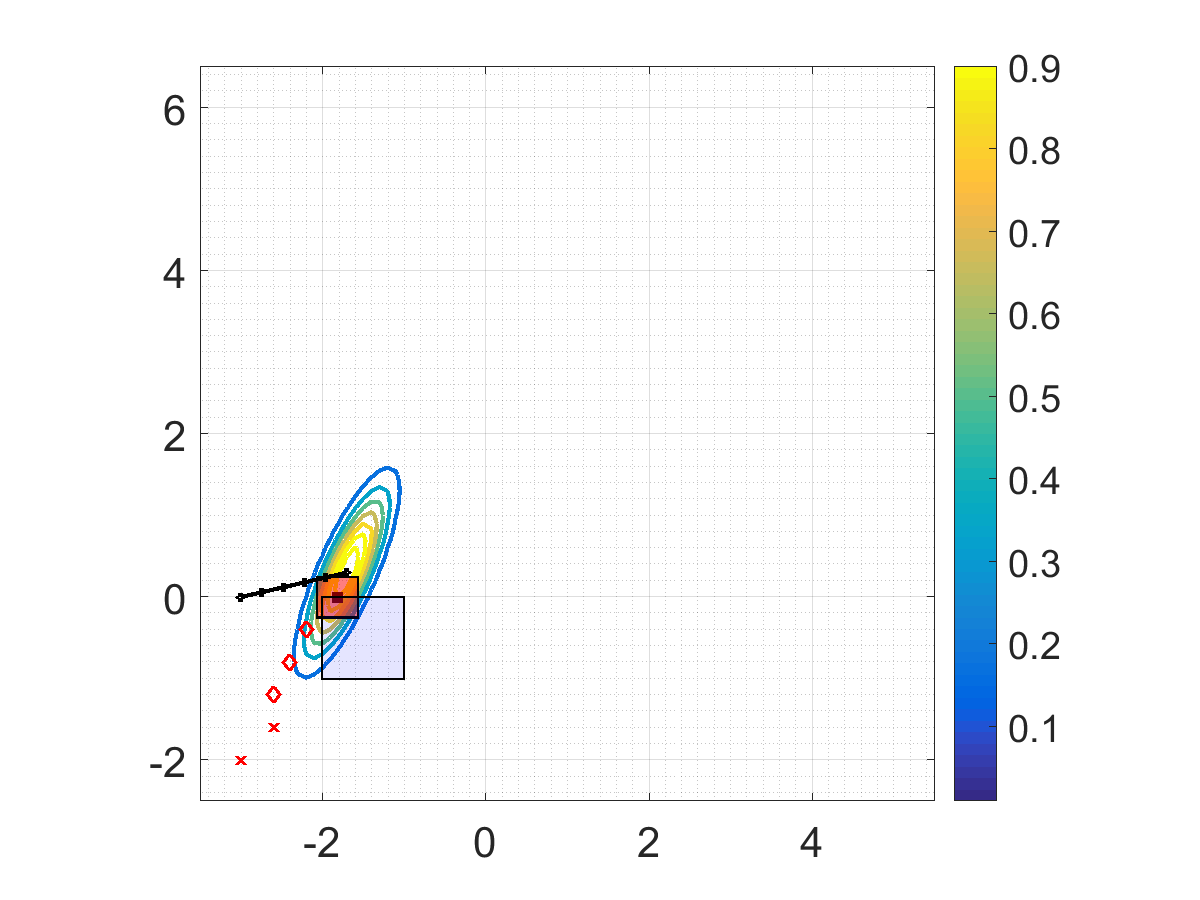
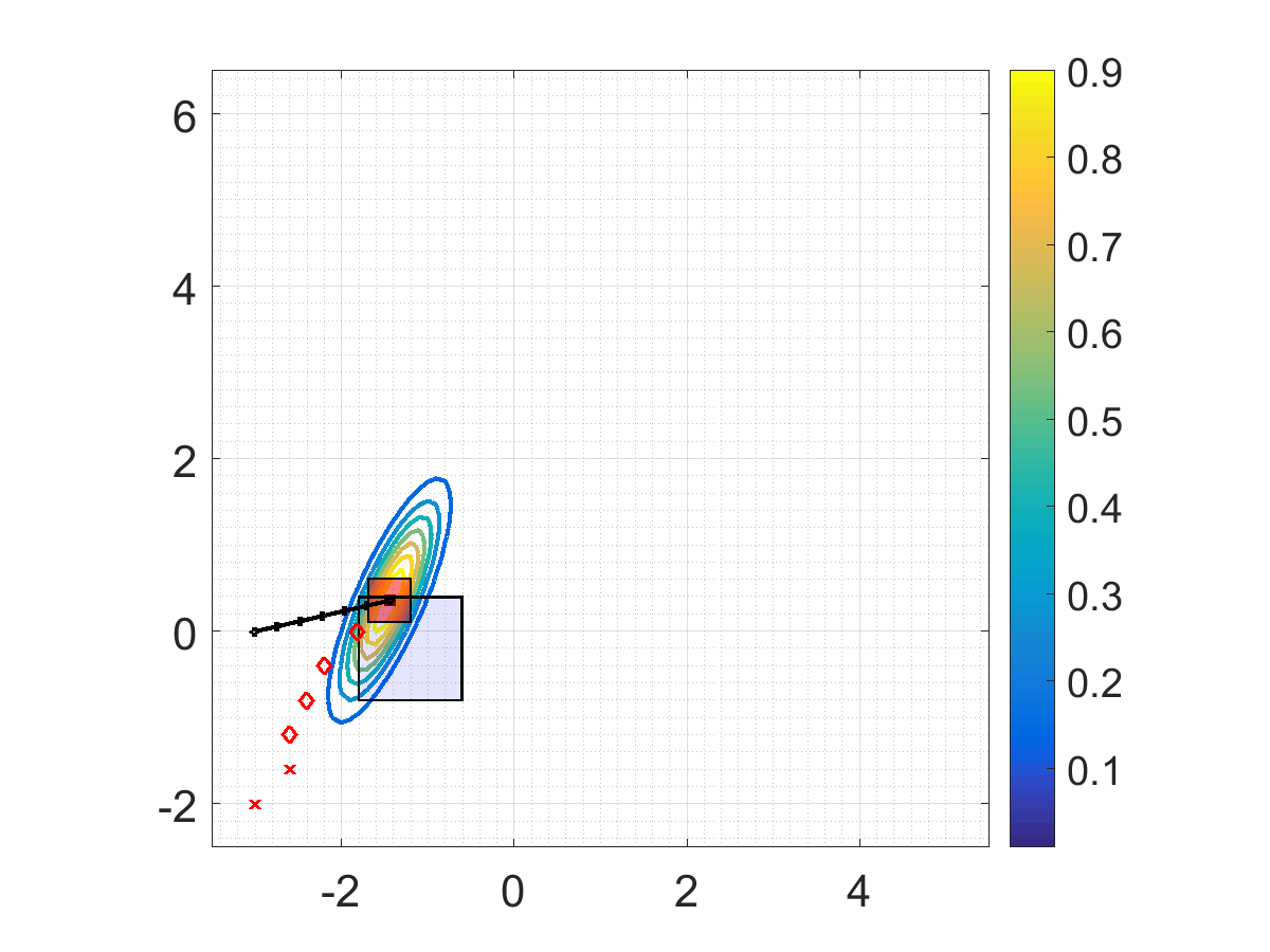
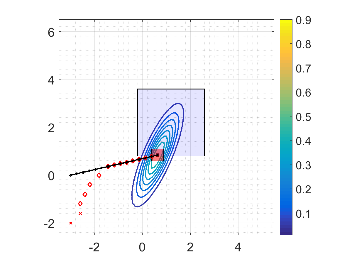
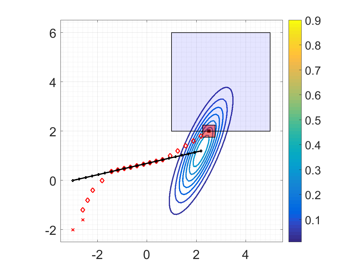
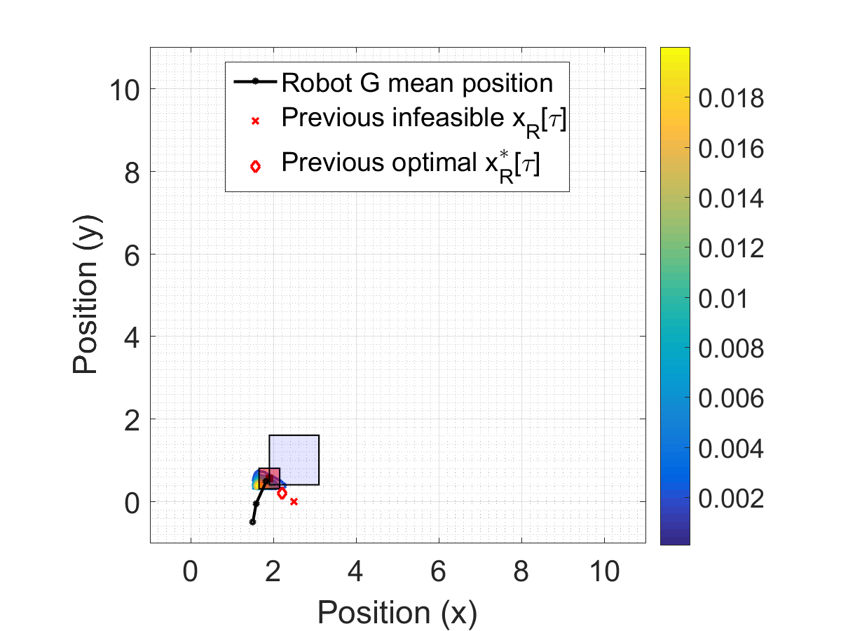
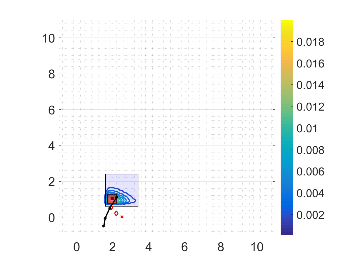
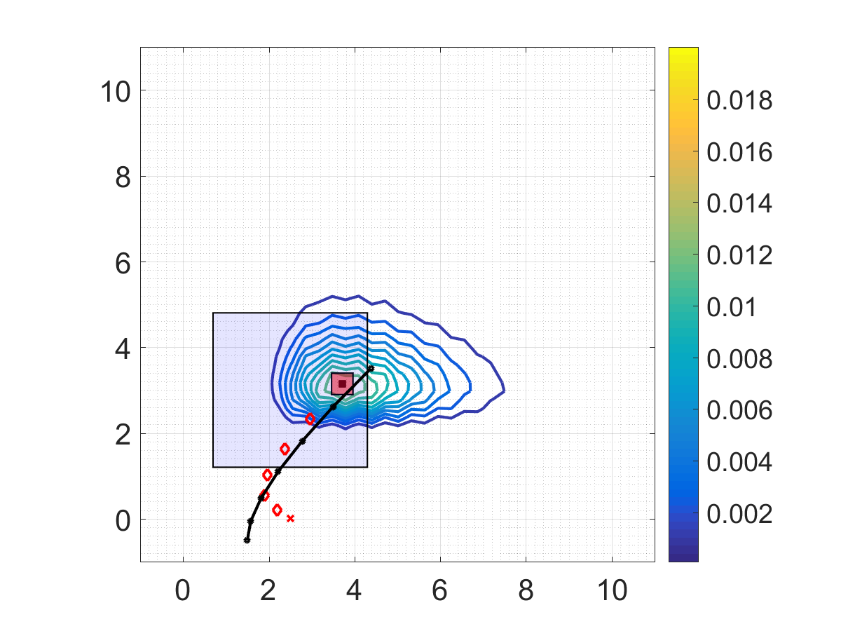
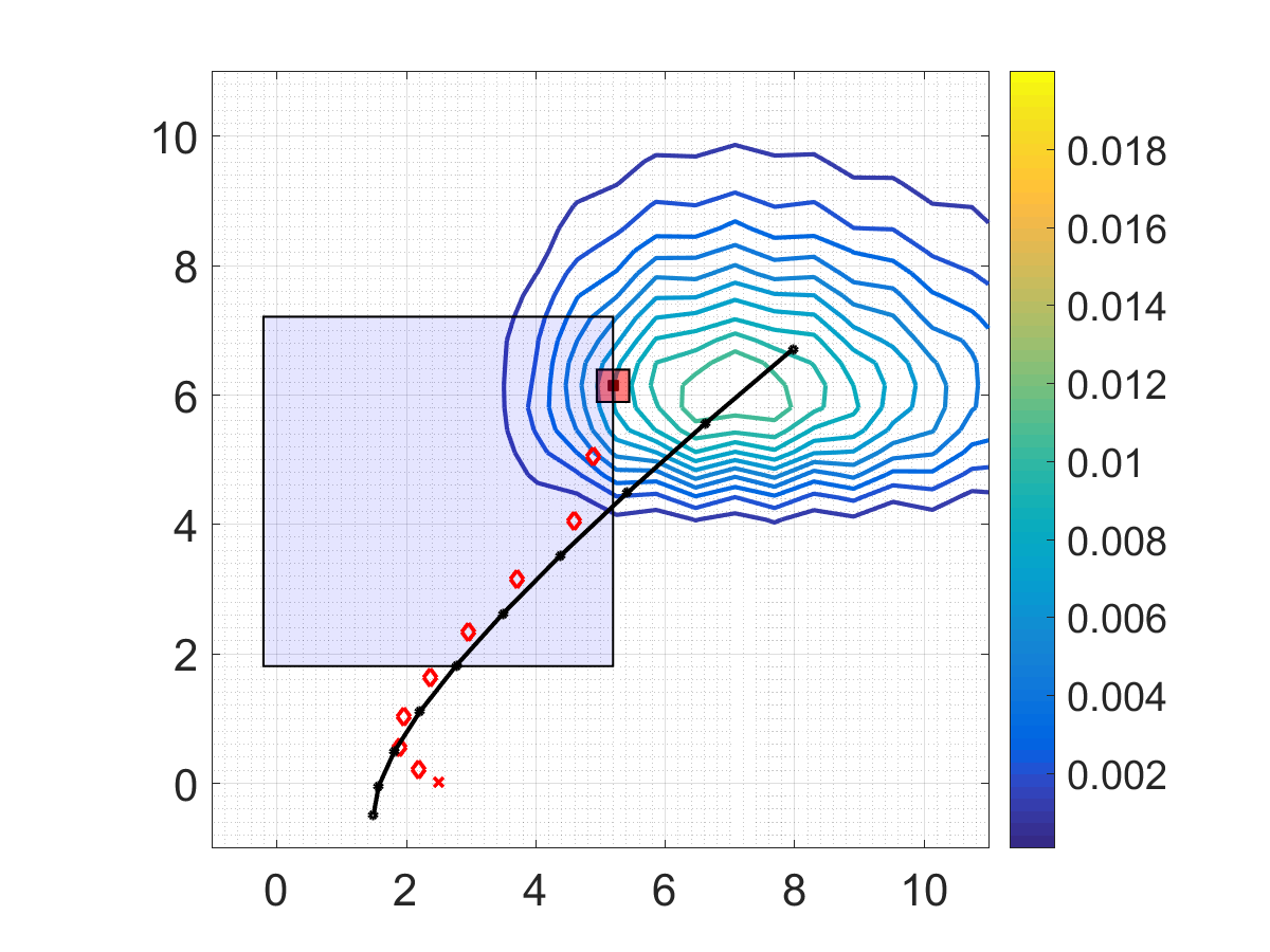
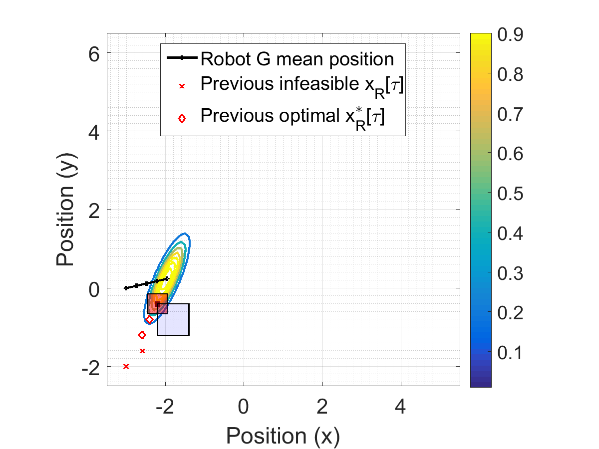
Figure 1: Snapshots of optimal capture positions of the robots G and R when G has point mass dynamics (23). The blue line shows the mean position trajectory of robot G μG[τ]subscript𝜇𝐺delimited-[]𝜏\mu_{G}[\tau], the contour plot characterizes ψ𝒙G(;τ,x¯G[0])subscript𝜓subscript𝒙𝐺𝜏subscript¯𝑥𝐺delimited-[]0\psi_{\boldsymbol{x}_{G}}(\cdot;\tau,\bar{x}_{G}[0]), the blue box shows the reach set of the robot R at time τ𝜏\tau ReachR(τ,x¯R[0])subscriptReach𝑅𝜏subscript¯𝑥𝑅delimited-[]0\mathrm{Reach}_{R}(\tau,\bar{x}_{R}[0]), and the red box shows the capture region centered at x¯R[τ]superscriptsubscript¯𝑥𝑅delimited-[]𝜏\bar{x}_{R}^{\ast}[\tau] CaptureSet(x¯R[τ])CaptureSetsuperscriptsubscript¯𝑥𝑅delimited-[]𝜏\mathrm{CaptureSet}(\bar{x}_{R}^{\ast}[\tau]).

4.1 Robot G with point mass dynamics
Refer to caption
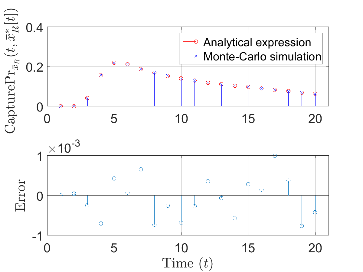
Figure 2: Solution to Problem ProbC for robot G dynamics in (23), and validation of CapturePrx¯R(τ,x¯R[τ];x¯G[0])subscriptCapturePrsubscript¯𝑥𝑅𝜏superscriptsubscript¯𝑥𝑅delimited-[]𝜏subscript¯𝑥𝐺delimited-[]0\mathrm{CapturePr}_{\bar{x}_{R}}(\tau,\bar{x}_{R}^{\ast}[\tau];\bar{x}_{G}[0]) via Monte-Carlo simulations. The optimal capture time is τ=5superscript𝜏5\tau^{\ast}=5 and the likelihood of capture is CapturePrx¯R(τ,x¯R[τ];x¯G[0])=0.219subscriptCapturePrsubscript¯𝑥𝑅superscript𝜏superscriptsubscript¯𝑥𝑅delimited-[]superscript𝜏subscript¯𝑥𝐺delimited-[]00.219\mathrm{CapturePr}_{\bar{x}_{R}}(\tau^{\ast},\bar{x}_{R}^{\ast}[\tau^{\ast}];\bar{x}_{G}[0])=0.219.

We solve Problem ProbB for the system given by (23). Here, the disturbance set is 𝒲=2𝒲superscript2\mathcal{W}=\mathbb{R}^{2}.

Lemma 6.

For the system given in (23) and initial state of the robot G as x¯G[0]2subscript¯𝑥𝐺delimited-[]0superscript2\bar{x}_{G}[0]\in\mathbb{R}^{2}, FSReachG(τ,x¯G[0])=2subscriptFSReach𝐺𝜏subscript¯𝑥𝐺delimited-[]0superscript2\mathrm{FSReach}_{G}(\tau,\bar{x}_{G}[0])=\mathbb{R}^{2} for every τ[1,T]𝜏1𝑇\tau\in[1,T].

Proof: Follows from Proposition 1 and (10).   

Proposition 1 provides the FSRPD and Lemma 6 provides the FSR set for the system (23). The probability of successful capture of the robot G can be computed using (31) since the FSRPD ψ𝒙G(;τ,x¯G[0])subscript𝜓subscript𝒙𝐺𝜏subscript¯𝑥𝐺delimited-[]0\psi_{\boldsymbol{x}_{G}}(\cdot;\tau,\bar{x}_{G}[0]) is available.

We implement the problem with the following parameters: Ts=0.2subscript𝑇𝑠0.2T_{s}=0.2, T=20𝑇20T=20, μ¯G𝒗=[1.3 0.3]superscriptsubscript¯𝜇𝐺𝒗superscriptdelimited-[]1.30.3top\bar{\mu}_{G}^{\boldsymbol{v}}=[1.3\ 0.3]^{\top}, ΣG=[0.50.80.82]subscriptΣ𝐺delimited-[]0.50.80.82\Sigma_{G}=\left[{\begin{array}[]{cc}0.5&0.8\\ 0.8&2\end{array}}\right], x¯G[0]=[3 0]subscript¯𝑥𝐺delimited-[]0superscriptdelimited-[]30top\bar{x}_{G}[0]=[-3\ 0]^{\top}, x¯R[0]=[32]subscript¯𝑥𝑅delimited-[]0superscriptdelimited-[]32top\bar{x}_{R}[0]=[-3\ -2]^{\top} and 𝒰=[1,2]2𝒰superscript122\mathcal{U}=[1,2]^{2}. The capture region of the robot R is a box centered about the position of the robot y¯¯𝑦\bar{y} with edge length 2a2𝑎2a (a=0.25𝑎0.25a=0.25) and edges parallel to the axes — CaptureSet(y¯)=Box(y¯,a)CaptureSet¯𝑦Box¯𝑦𝑎\mathrm{CaptureSet}(\bar{y})=\mathrm{Box}(\bar{y},a), a convex set. We use Jπ(π¯)=0subscript𝐽𝜋¯𝜋0J_{\pi}(\bar{\pi})=0 in Problem ProbD.

Figure 1 shows the evolution of the mean position of the robot G and the optimal capture position for the robot R at time instants 4,5,8,14,458144,5,8,14, and 202020. The contour plots of ψ𝒙G(;τ,x¯G[0])subscript𝜓subscript𝒙𝐺𝜏subscript¯𝑥𝐺delimited-[]0\psi_{\boldsymbol{x}_{G}}(\cdot;\tau,\bar{x}_{G}[0]) are rotated ellipses since ΣEsubscriptΣ𝐸\Sigma_{E} is not a diagonal matrix. From (17), the mean position of the robot G moves in a straight line μG[τ]subscript𝜇𝐺delimited-[]𝜏\mu_{G}[\tau], as it is the trajectory of (23a) when the input is always μ¯G𝒗superscriptsubscript¯𝜇𝐺𝒗\bar{\mu}_{G}^{\boldsymbol{v}}. The optimal time of capture is τ=5superscript𝜏5\tau^{\ast}=5, the optimal capture position is x¯R[τ]=[1.8 0]superscriptsubscript¯𝑥𝑅delimited-[]superscript𝜏superscriptdelimited-[]1.80top\bar{x}_{R}^{\ast}[\tau^{\ast}]=[-1.8\ 0]^{\top}, and the corresponding probability of robot R capturing robot G is 0.2190.2190.219. Note that at this instant, the reach set of the robot R does not cover the current mean position of the robot G, μ¯[τ]=[1.7 0.3]¯𝜇delimited-[]superscript𝜏superscriptdelimited-[]1.70.3top\bar{\mu}[\tau^{\ast}]=[-1.7\ 0.3]^{\top} (Figure 1b). While the reach set covers the mean position of robot G at the next time instant t=6𝑡6t=6, the uncertainty in (23) causes the probability of successful capture to further reduce (Figure 1c). Counterintuitively, attempting to reach the mean μG[τ]subscript𝜇𝐺delimited-[]𝜏\mu_{G}[\tau] is not always best. Figure 2 shows the optimal capture probabilities obtained when solving Problem ProbC for the dynamics (23).

4.2 Robot G with double integrator dynamics
Refer to caption
Time=1CapturePrx¯R=0(Infeasible)\begin{aligned} \mathrm{Time}&=1\\ \mathrm{CapturePr}_{\bar{x}_{R}}^{\ast}&=0\\ (\mbox{Inf}&\mbox{easible})\end{aligned}
Refer to caption
Time=2CapturePrx¯R=0.6044Timeabsent2superscriptsubscriptCapturePrsubscript¯𝑥𝑅absent0.6044\begin{aligned} \mathrm{Time}&=2\\ \mathrm{CapturePr}_{\bar{x}_{R}}^{\ast}&=0.6044\end{aligned}
Refer to caption
Time=3CapturePrx¯R=0.3885Timeabsent3superscriptsubscriptCapturePrsubscript¯𝑥𝑅absent0.3885\begin{aligned} \mathrm{Time}&=3\\ \mathrm{CapturePr}_{\bar{x}_{R}}^{\ast}&=0.3885\end{aligned}
Refer to caption
Time=6CapturePrx¯R=0.0495Timeabsent6superscriptsubscriptCapturePrsubscript¯𝑥𝑅absent0.0495\begin{aligned} \mathrm{Time}&=6\\ \mathrm{CapturePr}_{\bar{x}_{R}}^{\ast}&=0.0495\end{aligned}
Refer to caption
Time=9CapturePrx¯R=0.0091Timeabsent9superscriptsubscriptCapturePrsubscript¯𝑥𝑅absent0.0091\begin{aligned} \mathrm{Time}&=9\\ \mathrm{CapturePr}_{\bar{x}_{R}}^{\ast}&=0.0091\end{aligned}
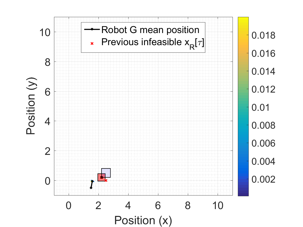
Figure 3: Snapshots of optimal capture positions of the robots G and R when G has double integrator dynamics (24). The blue line shows the mean position trajectory of robot G μG[τ]subscript𝜇𝐺delimited-[]𝜏\mu_{G}[\tau], the contour plot characterizes ψ𝒙Gpos(;τ,x¯G[0])superscriptsubscript𝜓subscript𝒙𝐺pos𝜏subscript¯𝑥𝐺delimited-[]0\psi_{\boldsymbol{x}_{G}}^{\mathrm{pos}}(\cdot;\tau,\bar{x}_{G}[0]) via Monte-Carlo simulation, the blue box shows the reach set of the robot R at time τ𝜏\tau, ReachR(τ,x¯R[0])subscriptReach𝑅𝜏subscript¯𝑥𝑅delimited-[]0\mathrm{Reach}_{R}(\tau,\bar{x}_{R}[0]), and the red box shows the capture region centered at x¯R[τ]superscriptsubscript¯𝑥𝑅delimited-[]𝜏\bar{x}_{R}^{\ast}[\tau], CaptureSet(x¯R[τ])CaptureSetsuperscriptsubscript¯𝑥𝑅delimited-[]𝜏\mathrm{CaptureSet}(\bar{x}_{R}^{\ast}[\tau]).
Refer to caption
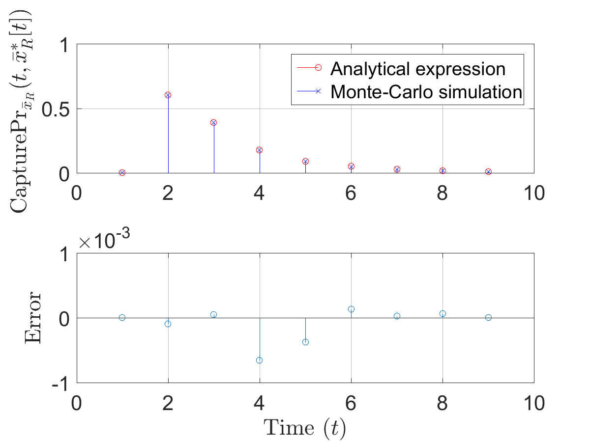
Figure 4: Solution to Problem ProbC for robot G dynamics in (24), and validation of CapturePrx¯R(τ,x¯R[τ];x¯G[0])subscriptCapturePrsubscript¯𝑥𝑅𝜏superscriptsubscript¯𝑥𝑅delimited-[]𝜏subscript¯𝑥𝐺delimited-[]0\mathrm{CapturePr}_{\bar{x}_{R}}(\tau,\bar{x}_{R}^{\ast}[\tau];\bar{x}_{G}[0]) via Monte-Carlo simulations. The optimal capture time is τ=2superscript𝜏2\tau^{\ast}=2 and the capture probability is CapturePrx¯R(τ,x¯R[τ];x¯G[0])=0.6044subscriptCapturePrsubscript¯𝑥𝑅superscript𝜏superscriptsubscript¯𝑥𝑅delimited-[]superscript𝜏subscript¯𝑥𝐺delimited-[]00.6044\mathrm{CapturePr}_{\bar{x}_{R}}(\tau^{\ast},\bar{x}_{R}^{\ast}[\tau^{\ast}];\bar{x}_{G}[0])=0.6044.

We now consider a more complicated capture problem, in which the disturbance is exponential (hence tracking the mean has little relevance because it is not the mode, the global maxima of the density), and the robot dynamics are more realistic. We solve Problem ProbB for the system given by (24). Here, the disturbance set is 𝒲=+2𝒲subscriptsuperscript2\mathcal{W}=\mathbb{R}^{2}_{+}. Based on the mean of the stochastic acceleration 𝒂[t]𝒂delimited-[]𝑡\boldsymbol{a}[t], the mean position of robot G has a parabolic trajectory due to the double integrator dynamics, as opposed to the linear trajectory seen in Subsection 4.1. Also, in this case, we do not have an explicit expression for the FSRPD like Proposition 1. Using Theorem 1, we obtain an explicit expression for the CF of the FSRPD. We utilize Lemma 1 to evaluate CapturePr()CapturePr\mathrm{CapturePr}(\cdot).

Analogous to Lemma 6 and Proposition 1, we characterize the FSR set in Lemma 7 and the FSRPD in Proposition 3. We use Lemma 3 to obtain an overapproximation of the FSR set due to the unavailability of FSRPD to use (10).

Lemma 7.

For the system given in (24) with initial state x¯G[0]4subscript¯𝑥𝐺delimited-[]0superscript4\bar{x}_{G}[0]\in\mathbb{R}^{4} of the robot G, we have FSReachG(τ,x¯G[0]){AG,DIτx¯G[0]}+4subscriptFSReach𝐺𝜏subscript¯𝑥𝐺delimited-[]0direct-sumsuperscriptsubscript𝐴GDI𝜏subscript¯𝑥𝐺delimited-[]0subscriptsuperscript4\mathrm{FSReach}_{G}(\tau,\bar{x}_{G}[0])\subseteq\{A_{\mathrm{G,DI}}^{\tau}\bar{x}_{G}[0]\}\oplus\mathbb{R}^{4}_{+} for every 2τT2𝜏𝑇2\leq\tau\leq T, and
FSReachG(1,x¯G[0]){AG,DIx¯G[0]}BG,DI+2subscriptFSReach𝐺1subscript¯𝑥𝐺delimited-[]0direct-sumsubscript𝐴GDIsubscript¯𝑥𝐺delimited-[]0subscript𝐵GDIsubscriptsuperscript2\mathrm{FSReach}_{G}(1,\bar{x}_{G}[0])\subseteq\{A_{\mathrm{G,DI}}\bar{x}_{G}[0]\}\oplus B_{\mathrm{G,DI}}\mathbb{R}^{2}_{+}.

Proof: For the dynamics in (24), 𝒞4×(2τ)+2τ=+4subscriptsuperscript𝒞top42𝜏subscriptsuperscript2𝜏subscriptsuperscript4\mathscr{C}^{\top}_{4\times(2{\tau})}\mathbb{R}^{2{\tau}}_{+}=\mathbb{R}^{4}_{+} since the rank of 𝒞4×(2τ)subscriptsuperscript𝒞top42𝜏\mathscr{C}^{\top}_{4\times(2{\tau})} is 4 for every τ2𝜏2{\tau}\geq 2, and elements of 𝒞4×(2τ)subscriptsuperscript𝒞top42𝜏\mathscr{C}^{\top}_{4\times(2\tau)} are nonnegative. For τ=1𝜏1{\tau}=1, 𝒞4×(2τ)=BG,DIsubscriptsuperscript𝒞top42𝜏subscript𝐵GDI\mathscr{C}^{\top}_{4\times(2\tau)}=B_{\mathrm{G,DI}}. Lemma 3 completes the proof.   

Proposition 3.

The CF of the FSRPD of the robot G for dynamics (24) is

Ψ𝒙G(β¯;τ,x¯G[0])subscriptΨsubscript𝒙𝐺¯𝛽𝜏subscript¯𝑥𝐺delimited-[]0\displaystyle\Psi_{\boldsymbol{x}_{G}}(\bar{\beta};\tau,\bar{x}_{G}[0]) =exp(jβ¯(AG,DIτx¯G[0]))×\displaystyle=\mathrm{exp}(j\bar{\beta}^{\top}(A^{\tau}_{\mathrm{G,DI}}\bar{x}_{G}[0]))\times
t=0τ1λaxλay(λaxjα¯2t)(λayjα¯2t+1)superscriptsubscriptproduct𝑡0𝜏1subscript𝜆axsubscript𝜆aysubscript𝜆ax𝑗subscript¯𝛼2𝑡subscript𝜆ay𝑗subscript¯𝛼2𝑡1\displaystyle\ \prod_{t=0}^{\tau-1}\frac{\lambda_{\mathrm{ax}}\lambda_{\mathrm{ay}}}{(\lambda_{\mathrm{ax}}-j\bar{\alpha}_{2t})(\lambda_{\mathrm{ay}}-j\bar{\alpha}_{2t+1})} (49)

where α¯=𝒞4×(2τ)β¯(2τ)¯𝛼superscriptsubscript𝒞42𝜏top¯𝛽superscript2𝜏\bar{\alpha}=\mathscr{C}_{4\times(2\tau)}^{\top}\bar{\beta}\in\mathbb{R}^{(2\tau)} and β¯4¯𝛽superscript4\bar{\beta}\in\mathbb{R}^{4}. The FSRPD of the robot G is ψ𝐱G(x¯;τ,x¯G[0])=1{Ψ𝐱G(;τ,x¯G[0])}(x¯)subscript𝜓subscript𝐱𝐺¯𝑥𝜏subscript¯𝑥𝐺delimited-[]0superscript1subscriptΨsubscript𝐱𝐺𝜏subscript¯𝑥𝐺delimited-[]0¯𝑥\psi_{\boldsymbol{x}_{G}}(\bar{x};\tau,\bar{x}_{G}[0])=\mathscr{F}^{-1}\big{\{}\Psi_{\boldsymbol{x}_{G}}(\cdot;\tau,\bar{x}_{G}[0])\big{\}}(-\bar{x}).

Proof: Apply Theorem 1 to the dynamics (24).   

To solve Problem ProbB, we define CapturePrx¯R()subscriptCapturePrsubscript¯𝑥𝑅\mathrm{CapturePr}_{\bar{x}_{R}}(\cdot) as in (31). Since we are interested in just the position of robot G, we require only the marginal density of the FSRPD over the position subspace of robot G, ψ𝒙Gpossuperscriptsubscript𝜓subscript𝒙𝐺pos\psi_{\boldsymbol{x}_{G}}^{\mathrm{pos}}. By Property P4, we have for γ¯=[γ1γ2]2¯𝛾delimited-[]subscript𝛾1subscript𝛾2superscript2\bar{\gamma}=[\gamma_{1}\ \gamma_{2}]\in\mathbb{R}^{2},

Ψ𝒙Gpos(γ¯;τ,x¯G[0])superscriptsubscriptΨsubscript𝒙𝐺pos¯𝛾𝜏subscript¯𝑥𝐺delimited-[]0\displaystyle\Psi_{\boldsymbol{x}_{G}}^{\mathrm{pos}}(\bar{\gamma};\tau,\bar{x}_{G}[0]) =Ψ𝒙G([γ1 0γ2 0];τ,x¯G[0]).absentsubscriptΨsubscript𝒙𝐺superscriptdelimited-[]subscript𝛾1 0subscript𝛾2 0top𝜏subscript¯𝑥𝐺delimited-[]0\displaystyle=\Psi_{\boldsymbol{x}_{G}}({[\gamma_{1}\ 0\ \gamma_{2}\ 0]}^{\top};\tau,\bar{x}_{G}[0]). (50)

Unlike the case with Gaussian disturbance, explicit expressions for the FSRPD ψ𝒙Gsubscript𝜓subscript𝒙𝐺\psi_{\boldsymbol{x}_{G}} or its marginal density ψ𝒙Gpossuperscriptsubscript𝜓subscript𝒙𝐺pos\psi_{\boldsymbol{x}_{G}}^{\mathrm{pos}} are unavailable since the Fourier transform (49) is not standard.

Lemma 8.

ψBG,DI𝒂,ψ𝒙GL1(4)L2(4)subscript𝜓subscript𝐵GDI𝒂subscript𝜓subscript𝒙𝐺superscript𝐿1superscript4superscript𝐿2superscript4\psi_{B_{\mathrm{G,DI}}\boldsymbol{a}},\ \psi_{\boldsymbol{x}_{G}}\in L^{1}(\mathbb{R}^{4})\cap L^{2}(\mathbb{R}^{4}).

Proof: (For ψBG,DI𝐚subscript𝜓subscript𝐵GDI𝐚\psi_{B_{\mathrm{G,DI}}\boldsymbol{a}}) By Hölder’s inequality[22, Section 19], ψ𝒂L1(2)L2(2)subscript𝜓𝒂superscript𝐿1superscript2superscript𝐿2superscript2\psi_{\boldsymbol{a}}\in L^{1}(\mathbb{R}^{2})\cap L^{2}(\mathbb{R}^{2}). We also have
ψBG,DI𝒂(z1,z2,z3,z4)=δ(z3Tsz42)δ(z1Tsz22)ψ𝒛24(z2,z4)subscript𝜓subscript𝐵GDI𝒂subscript𝑧1subscript𝑧2subscript𝑧3subscript𝑧4𝛿subscript𝑧3subscript𝑇𝑠subscript𝑧42𝛿subscript𝑧1subscript𝑇𝑠subscript𝑧22subscript𝜓subscript𝒛24subscript𝑧2subscript𝑧4\psi_{B_{\mathrm{G,DI}}\boldsymbol{a}}(z_{1},z_{2},z_{3},z_{4})=\delta(z_{3}-\frac{T_{s}z_{4}}{2})\delta(z_{1}-\frac{T_{s}z_{2}}{2})\psi_{\boldsymbol{z}_{24}}(z_{2},z_{4}) where 𝒛24=[z2z4]=Ts𝒂2subscript𝒛24superscriptdelimited-[]subscript𝑧2subscript𝑧4topsubscript𝑇𝑠𝒂superscript2\boldsymbol{z}_{24}=[z_{2}\ z_{4}]^{\top}=T_{s}\boldsymbol{a}\in\mathbb{R}^{2} and ψ𝒛24(z2,z4)=Ts2ψ𝒂(z2Ts,z4Ts)subscript𝜓subscript𝒛24subscript𝑧2subscript𝑧4superscriptsubscript𝑇𝑠2subscript𝜓𝒂subscript𝑧2subscript𝑇𝑠subscript𝑧4subscript𝑇𝑠\psi_{\boldsymbol{z}_{24}}(z_{2},z_{4})=T_{s}^{-2}\psi_{\boldsymbol{a}}(\frac{z_{2}}{T_{s}},\frac{z_{4}}{T_{s}}) from (12). For i={1,2}𝑖12i=\{1,2\}, ψBG,DI𝒂i=ψ𝒛24i=Ts22iψ𝒂i<subscriptnormsubscript𝜓subscript𝐵GDI𝒂𝑖subscriptnormsubscript𝜓subscript𝒛24𝑖superscriptsubscript𝑇𝑠22𝑖subscriptnormsubscript𝜓𝒂𝑖{\|\psi_{B_{\mathrm{G,DI}}\boldsymbol{a}}\|}_{i}={\|\psi_{\boldsymbol{z}_{24}}\|}_{i}=T_{s}^{2-2i}{\|\psi_{\boldsymbol{a}}\|}_{i}<\infty completing the proof.

(For ψ𝐱Gsubscript𝜓subscript𝐱𝐺\psi_{\boldsymbol{x}_{G}}) Via induction using (11) (similar to the proof of Theorem 2). Note that functions in L1(4)L2(4)superscript𝐿1superscript4superscript𝐿2superscript4L^{1}(\mathbb{R}^{4})\cap L^{2}(\mathbb{R}^{4}) are closed under convolution [26, Theorem 1.3].   

Lemma 9.

ψ𝒙Gpos(x¯;τ,x¯G[0])L1(2)L2(2)superscriptsubscript𝜓subscript𝒙𝐺pos¯𝑥𝜏subscript¯𝑥𝐺delimited-[]0superscript𝐿1superscript2superscript𝐿2superscript2\psi_{\boldsymbol{x}_{G}}^{\mathrm{pos}}(\bar{x};\tau,\bar{x}_{G}[0])\in L^{1}(\mathbb{R}^{2})\cap L^{2}(\mathbb{R}^{2}).

Proof: For i={1,2}𝑖12i=\{1,2\}, we have from (50), ψ𝒙Gposi=ψ𝒙Gisubscriptnormsuperscriptsubscript𝜓subscript𝒙𝐺pos𝑖subscriptnormsubscript𝜓subscript𝒙𝐺𝑖{\|\psi_{\boldsymbol{x}_{G}}^{\mathrm{pos}}\|}_{i}={\|\psi_{\boldsymbol{x}_{G}}\|}_{i}, and from Lemma 8, ψ𝒙Gi<subscriptnormsubscript𝜓subscript𝒙𝐺𝑖{\|\psi_{\boldsymbol{x}_{G}}\|}_{i}<\infty.   

Similar to Subsection 4.1, we define a convex capture region CaptureSet(y¯R)=Box(y¯R,a)2CaptureSetsubscript¯𝑦𝑅Boxsubscript¯𝑦𝑅𝑎superscript2\mathrm{CaptureSet}(\bar{y}_{R})=\mathrm{Box}(\bar{y}_{R},a)\subseteq\mathbb{R}^{2} where y¯R2subscript¯𝑦𝑅superscript2\bar{y}_{R}\in\mathbb{R}^{2} is the state of the robot R. We define h(y¯;y¯R,a)=𝟏Box(y¯R,a)(y¯)¯𝑦subscript¯𝑦𝑅𝑎subscript1Boxsubscript¯𝑦𝑅𝑎¯𝑦h(\bar{y};\bar{y}_{R},a)=\mathbf{1}_{\mathrm{Box}(\bar{y}_{R},a)}(\bar{y}) as the indicator function corresponding to a 222-D box centered at y¯Rsubscript¯𝑦𝑅\bar{y}_{R} with edge length 2a>02𝑎02a>0 with h(y¯)=1¯𝑦1h(\bar{y})=1 if y¯CaptureSet(y¯R)¯𝑦CaptureSetsubscript¯𝑦𝑅\bar{y}\in\mathrm{CaptureSet}(\bar{y}_{R}) and zero otherwise. The Fourier transform of hh is a product of sinc functions shifted by y¯Rsubscript¯𝑦𝑅\bar{y}_{R} (follows from Property P2 and [30, Chapter 13])

H(γ¯;y¯R,a)𝐻¯𝛾subscript¯𝑦𝑅𝑎\displaystyle H(\bar{\gamma};\bar{y}_{R},a) ={h(;y¯R,a)}(γ¯)absentsubscript¯𝑦𝑅𝑎¯𝛾\displaystyle=\mathscr{F}\{h(\cdot;\bar{y}_{R},a)\}(\bar{\gamma})
=4a2exp(jy¯Rγ¯)sin(aγ1)sin(aγ2)γ1γ2.absent4superscript𝑎2𝑗superscriptsubscript¯𝑦𝑅top¯𝛾𝑎subscript𝛾1𝑎subscript𝛾2subscript𝛾1subscript𝛾2\displaystyle=4a^{2}\exp{(-j\bar{y}_{R}^{\top}\bar{\gamma})}\frac{\sin(a\gamma_{1})\sin(a\gamma_{2})}{\gamma_{1}\gamma_{2}}. (51)

Clearly, hh is square-integrable, and from Lemmas 1 and 9, we define CapturePrx¯R()subscriptCapturePrsubscript¯𝑥𝑅\mathrm{CapturePr}_{\bar{x}_{R}}(\cdot) in (53). Equation (53) is evaluated using (49), (50), and (51). We use (53) as opposed (52) due to the unavailability of an explicit expression for ψ𝒙Gpossuperscriptsubscript𝜓subscript𝒙𝐺pos\psi_{\boldsymbol{x}_{G}}^{\mathrm{pos}}. The numerical evaluation of the inverse Fourier transform of Ψ𝒙GpossuperscriptsubscriptΨsubscript𝒙𝐺pos\Psi_{\boldsymbol{x}_{G}}^{\mathrm{pos}} to compute (52) will require two quadratures, resulting in a higher approximation error as compared to (53).

CapturePrx¯R(τ,x¯R[τ];x¯G[0])subscriptCapturePrsubscript¯𝑥𝑅𝜏subscript¯𝑥𝑅delimited-[]𝜏subscript¯𝑥𝐺delimited-[]0\displaystyle\mathrm{CapturePr}_{\bar{x}_{R}}(\tau,\bar{x}_{R}[\tau];\bar{x}_{G}[0]) =2ψ𝒙Gpos(x¯;τ,x¯G[0])h(x¯;x¯R[τ],a)𝑑x¯absentsubscriptsuperscript2superscriptsubscript𝜓subscript𝒙𝐺pos¯𝑥𝜏subscript¯𝑥𝐺delimited-[]0¯𝑥subscript¯𝑥𝑅delimited-[]𝜏𝑎differential-d¯𝑥\displaystyle=\int_{\mathbb{R}^{2}}\psi_{\boldsymbol{x}_{G}}^{\mathrm{pos}}(\bar{x};\tau,\bar{x}_{G}[0])h(\bar{x};\bar{x}_{R}[\tau],a)d\bar{x} (52)
=(12π)22Ψ𝒙Gpos(γ¯;τ,x¯G[0])H(γ¯;x¯R[τ],a)𝑑γ¯.absentsuperscript12𝜋2subscriptsuperscript2superscriptsubscriptΨsubscript𝒙𝐺pos¯𝛾𝜏subscript¯𝑥𝐺delimited-[]0𝐻¯𝛾subscript¯𝑥𝑅delimited-[]𝜏𝑎differential-d¯𝛾\displaystyle={\left(\frac{1}{2\pi}\right)}^{2}\int_{\mathbb{R}^{2}}\Psi_{\boldsymbol{x}_{G}}^{\mathrm{pos}}(\bar{\gamma};\tau,\bar{x}_{G}[0])H(\bar{\gamma};\bar{x}_{R}[\tau],a)d\bar{\gamma}. (53)


We implement the problem with the following parameters: Ts=0.2subscript𝑇𝑠0.2T_{s}=0.2, T=9𝑇9T=9, a=0.25𝑎0.25a=0.25, λax=0.25subscript𝜆ax0.25\lambda_{\mathrm{ax}}=0.25, λay=0.45subscript𝜆ay0.45\lambda_{\mathrm{ay}}=0.45, x¯G[0]=[1.5 00.5 2]subscript¯𝑥𝐺delimited-[]0superscriptdelimited-[]1.500.52top\bar{x}_{G}[0]={[1.5\ 0\ -0.5\ 2]}^{\top}, x¯R[0]=[2.5 0]subscript¯𝑥𝑅delimited-[]0superscriptdelimited-[]2.50top\bar{x}_{R}[0]=[2.5\ 0]^{\top}, and 𝒰=[1.5,1.5]×[1,4]𝒰1.51.514\mathcal{U}=[-1.5,1.5]\times[1,4]. We use Jπ(π¯)=0subscript𝐽𝜋¯𝜋0J_{\pi}(\bar{\pi})=0 in Problem ProbD.

Figure 3 shows the evolution of the mean position of the robot G and the optimal capture position for the robot R at time instants 1,2,3,6,12361,2,3,6, and 999. For every τ[1,T]𝜏1𝑇\tau\in[1,T], the contour plots of ψ𝒙Gpos(;τ,x¯G[0])superscriptsubscript𝜓subscript𝒙𝐺pos𝜏subscript¯𝑥𝐺delimited-[]0\psi_{\boldsymbol{x}_{G}}^{\mathrm{pos}}(\cdot;\tau,\bar{x}_{G}[0]) were estimated via Monte-Carlo simulation since evaluating ψ𝒙Gpos(;τ,x¯G[0])superscriptsubscript𝜓subscript𝒙𝐺pos𝜏subscript¯𝑥𝐺delimited-[]0\psi_{\boldsymbol{x}_{G}}^{\mathrm{pos}}(\cdot;\tau,\bar{x}_{G}[0]) via (5) over a grid is computationally expensive. Note that the mean position of the robot G does not coincide with the mode of ψ𝒙Gpos(;τ,x¯G[0])superscriptsubscript𝜓subscript𝒙𝐺pos𝜏subscript¯𝑥𝐺delimited-[]0\psi_{\boldsymbol{x}_{G}}^{\mathrm{pos}}(\cdot;\tau,\bar{x}_{G}[0]) in contrast to the problem discussed in Subsection 4.1. The optimal time of capture is at τ=2superscript𝜏2\tau^{\ast}=2, the optimal capture position is x¯R[τ]=[1.9 0.55]superscriptsubscript¯𝑥𝑅delimited-[]superscript𝜏superscriptdelimited-[]1.90.55top\bar{x}_{R}^{\ast}[\tau^{\ast}]=[1.9\ 0.55]^{\top}, and the corresponding probability of robot R capturing robot G is 0.60440.60440.6044 (Figure 3b). Figure 4 shows the optimal capture probabilities obtained when solving Problem ProbC for the dynamics (24), and the validation of the results.

4.3 Numerical implementation and analysis

All computations in this paper were performed using MATLAB on an Intel Core i7 CPU with 3.4GHz clock rate and 16 GB RAM. The MATLAB code for this work is available at http://hscl.unm.edu/files/code/HSCC17.zip.

We solved Problem ProbC using MATLAB’s built-in functions — fmincon for the optimization, mvncdf to compute the objective (31) for the case in Subsection 4.1, integral to compute the objective (53) for the case in Subsection 4.2, and max to compute the global optimum of Problem ProbB. In both the sections, we used MPT for the reachable set calculation and solved Problem ProbD using CVX [36]. Using Lemma 2, the FSR sets restrict the search while solving Problem ProbC. All geometric computations were done in the facet representation. We computed the initial guess for the optimization of Problem ProbC by performing Euclidean projection of the mean to the feasible set using CVX [34, Section 8.1.1]. Since computing the objective was costly, this operation saved significant computational time. The Monte-Carlo simulation used 500,000500000500,000 particles. No offline computations were done in either of the cases.

The overall computation of Problem ProbB and ProbD for the case in Subsection 4.1 took 5.325.325.32 seconds for T=20𝑇20T=20. Since Proposition 1 provides explicit expressions for the FSRPD, the evaluation of the FSRPD for any given point y¯𝒳¯𝑦𝒳\bar{y}\in\mathcal{X} takes 1.61.61.6 millseconds on average. For the case in Subsection 4.2, the overall computation took 488.55488.55488.55 seconds (8similar-toabsent8\sim 8 minutes) for T=9𝑇9T=9. The numerical evaluation of the improper integral (53) is the major cause of increase in runtime. The evaluation of the FSRPD for any given point y¯𝒳¯𝑦𝒳\bar{y}\in\mathcal{X} using (5) takes about 10.510.510.5 seconds, and the runtime and the accuracy depend heavily on the point y¯¯𝑦\bar{y} as well as the bounds used for the integral approximation. However, the evaluation of CapturePrx¯R()subscriptCapturePrsubscript¯𝑥𝑅\mathrm{CapturePr}_{\bar{x}_{R}}(\cdot) using (53) is much faster (0.810.810.81 seconds) because H(γ¯;y¯R,a)𝐻¯𝛾subscript¯𝑦𝑅𝑎H(\bar{\gamma};\bar{y}_{R},a) is a decaying, 2-D sinc function (decaying much faster than the CF).

The decaying properties of the integrand in (53) and CFs in general permits approximating the improper integrals in (5) and (53) by as a proper integral with suitably defined finite bounds. The tradeoff between accuracy and computational speed, common in quadrature techniques, dictates the choice of the bound. A detailed analysis of various quadrature techniques, their computational complexity, and their error analysis can be found in [31, Chapter 4].

5 Conclusions and Future work

This paper provides a method for forward stochastic reachability analysis using Fourier transforms. The method is applicable to uncontrolled stochastic linear systems. Fourier transforms simplify the computation and mitigate the curse of dimensionality associated with gridding the state space. We also analyze several convexity results associated with the FSRPD and FSR sets. We demonstrate our method on the problem of controller synthesis for a controlled robot pursuing a stochastically moving non-adversarial target.

Future work includes exploration of various quadrature techniques like particle filters for high-dimensional quadratures, and extension to a model predictive control framework and to discrete random vectors (countable disturbance sets). Multiple pursuer applications will also be investigated.

6 Acknowledgements

The authors thank Prof. M. Hayat for discussions on Fourier transforms in probability theory and the reviewers for their insightful comments.

This material is based upon work supported by the National Science Foundation, under Grant Numbers CMMI-1254990, CNS-1329878, and IIS-1528047. Any opinions, findings, and conclusions or recommendations expressed in this material are those of the authors and do not necessarily reflect the views of the National Science Foundation.

References

  • [1] Baisravan HomChaudhuri, Abraham P. Vinod, and Meeko M. K. Oishi. Computation of forward stochastic reach sets: Application to stochastic, dynamic obstacle avoidance. In Proc. American Control Conf., 2017. (accepted).
  • [2] Nick Malone, Kendra Lesser, Meeko Oishi, and Lydia Tapia. Stochastic reachability based motion planning for multiple moving obstacle avoidance. In Proc. Hybrid Syst.: Comput. and Control, pages 51–60, 2014.
  • [3] Kendra Lesser, Meeko Oishi, and R. Scott Erwin. Stochastic reachability for control of spacecraft relative motion. In Proc. IEEE Conf. on Decision and Control, pages 4705–4712, 2013.
  • [4] Sean Summers and John Lygeros. Verification of discrete time stochastic hybrid systems: A stochastic reach-avoid decision problem. Automatica, 46(12):1951–1961, 2010.
  • [5] Nikolaos Kariotoglou, Davide M Raimondo, Sean Summers, and John Lygeros. A stochastic reachability framework for autonomous surveillance with pan-tilt-zoom cameras. In European Control Conf., pages 1411–1416, 2011.
  • [6] Alessandro Abate, Maria Prandini, John Lygeros, and Shankar Sastry. Probabilistic reachability and safety for controlled discrete time stochastic hybrid systems. Automatica, 44(11):2724–2734, 2008.
  • [7] Alessandro Abate, Saurabh Amin, Maria Prandini, John Lygeros, and Shankar Sastry. Computational approaches to reachability analysis of stochastic hybrid systems. In Proc. Hybrid Syst.: Comput. and Control, pages 4–17, 2007.
  • [8] Nikolaos Kariotoglou, Sean Summers, Tyler Summers, Maryam Kamgarpour, and John Lygeros. Approximate dynamic programming for stochastic reachability. In European Control Conf., pages 584–589, 2013.
  • [9] Nikolaos Kariotoglou, Kostas Margellos, and John Lygeros. On the computational complexity and generalization properties of multi-stage and stage-wise coupled scenario programs. Syst. and Control Lett., 94:63–69, 2016.
  • [10] Giorgio Manganini, Matteo Pirotta, Marcello Restelli, Luigi Piroddi, and Maria Prandini. Policy search for the optimal control of Markov Decision Processes: A novel particle-based iterative scheme. IEEE Trans. Cybern., pages 1–13, 2015.
  • [11] Michal Kvasnica, Bálint Takács, Juraj Holaza, and Deepak Ingole. Reachability analysis and control synthesis for uncertain linear systems in MPT. IFAC Symp. on Robust Control D., 48(14):302–307, 2015.
  • [12] Alex A. Kurzhanskiy and Pravin Varaiya. Ellipsoidal toolbox. Technical Report UCB/EECS-2006-46, EECS Department, University of California, Berkeley, 2006.
  • [13] Antoine Girard. Reachability of uncertain linear systems using zonotopes. In Proc. Hybrid Syst.: Comput. and Control, pages 291–305, 2005.
  • [14] Geoffrey Hollinger, Sanjiv Singh, Joseph Djugash, and Athanasios Kehagias. Efficient multi-robot search for a moving target. Int’l J. Robotics and Research, 28(2):201–219, 2009.
  • [15] Vijay Kumar, Daniela Rus, and Sanjiv Singh. Robot and sensor networks for first responders. IEEE Pervasive computing, 3(4):24–33, 2004.
  • [16] Christopher Geyer. Active target search from UAVs in urban environments. In Proc. IEEE Int’l Conf. Robotics and Autom., pages 2366–2371, 2008.
  • [17] Ian Mitchell and Claire J. Tomlin. Level set methods for computation in hybrid systems. In Proc. Hybrid Syst.: Comput. and Control, pages 310–323, 2000.
  • [18] Claire J. Tomlin, John Lygeros, and Shankar Sastry. A game theoretic approach to controller design for hybrid systems. Proc. IEEE, 88(7):949–970, 2000.
  • [19] Claire J. Tomlin, Ian Mitchell, Alexandre M. Bayen, and Meeko Oishi. Computational techniques for the verification of hybrid systems. Proc. IEEE, 91(7):986–1001, 2003.
  • [20] Olivier Bokanowski, Nicolas Forcadel, and Hasnaa Zidani. Reachability and Minimal Times for State Constrained Nonlinear Problems without Any Controllability Assumption. SIAM J. of Control and Optimization, 48(7):4292–4316, 2010.
  • [21] Haomiao Huang, Jerry Ding, Wei Zhang, and Claire J. Tomlin. Automation-assisted capture-the-flag: A differential game approach. IEEE Trans. Control Syst. Technol., 23:1014–1028, 2015.
  • [22] Patrick Billingsley. Probability and measure. Wiley, New York, 3 edition, 1995.
  • [23] John A Gubner. Probability and random processes for electrical and computer engineers. Cambridge University Press, New York; Cambridge, 2006.
  • [24] Harald Cramér. Mathematical methods of statistics (PMS-9). Princeton university press, 9 edition, 1961.
  • [25] Sudhakar Dharmadhikari and Kumar Joag-Dev. Unimodality, convexity, and applications. Elsevier, 1988.
  • [26] Elias M Stein and Guido L Weiss. Introduction to Fourier analysis on Euclidean spaces, volume 1. Princeton University Press, 1971.
  • [27] Terence Tao. Analysis II. Hindustan Book Agency, 2 edition, 2009.
  • [28] Jean-Paul Penot. Analysis: From Concepts to Applications. Springer, 1 edition, 2016.
  • [29] Andrzej Lasota and Michael C Mackey. Chaos, fractals, and noise: stochastic aspects of dynamics, volume 97. Springer Science & Business Media, 2013.
  • [30] Ron Bracewell. The Fourier transform and its applications. McGraw-Hill, Inc., 1986.
  • [31] William H. Press, Saul A. Teukolsky, William T. Vetterling, and Brian P. Flannery. Numerical recipes: The art of scientific computing. Cambridge University Press, New York, NY, USA, 3 edition, 2007.
  • [32] Peter Dorato, Vito Cerone, and Chaouki Abdallah. Linear-quadratic control: An introduction. Simon & Schuster, 1994.
  • [33] Y.S. Chow and H. Teicher. Probability Theory: Independence, Interchangeability, Martingales. Springer Texts in Statistics. Springer New York, 1997.
  • [34] Stephen P. Boyd and Lieven Vandenberghe. Convex optimization. Cambridge University Press, Cambridge, UK ; New York, 2004.
  • [35] Martin Herceg, Michal Kvasnica, Colin N. Jones, and Manfred Morari. Multi-Parametric Toolbox 3.0. In European Control Conf., pages 502–510, 2013. http://control.ee.ethz.ch/~mpt.
  • [36] Michael Grant and Stephen Boyd. CVX: MATLAB software for disciplined convex programming, version 2.1. http://cvxr.com/cvx, 2014.