Compensating strong coupling with large charge

1 Introduction and Conclusions

The slightly provocative title of this paper refers to the very intriguing results presented in [1] where the anomalous dimensions of operators with large global charge $J$ in certain cft in three-dimensions were obtained. In most cft, the description in terms of local Lagrangians is not adequate, because the theory is frequently strongly coupled, and thus, the perturbative description is not valid. However, if the theory has some global symmetry group, and if we consider it in the sector with large values of the associated charges, the effective theory describing those operators is found to be effectively at weak couplings. In such a regime, quite universal results can be obtained for the anomalous dimensions of the operators. This paper is a first attempt to understand the generality of these results.

It is well known that Goldstone’s theorem presents a far richer phenomenology when the theory is non-relativistic [2, 3] (see also the review [4], and [5]). The counting of Goldstone bosons and their dispersion relations is more elaborate. In fact, if we consider relativistic field theories like qcd (qcd) with non-zero chemical potential for global symmetries, (see for instance [6]) we have to consider the theory in a non-relativistic context, and the low-energy excitations follow the more general form of Goldstone’s theorem. Relativistic theories in the sector of fixed global charges have been also studied in the past [6, 7, 8, 9], and it is interesting that Type I and II Goldstone bosons appear in general.

The aim of this paper is to show that when we consider quantum field theories with global symmetries, and we study the sector of the Hilbert space of states with large values of the global charge, we find not only that generically there are Goldstone excitations in the effective Lagrangian describing that sector of the theory, but furthermore, it seems that the effective couplings are related to the original couplings but suppressed by powers of the global charge. Hence the larger the charge, the weaker the coupling and thus the more reliable the results obtained in perturbation theory.

In this paper, we consider the case of the $O(N)$ vector model. Two particular results to be stressed are that

1. a homogeneous fixed-charge ground state (spin-$0$ operator) is only possible for a specific choice of the $O(N)$ weights;

2. the light spectrum of the theory around the large-charge ground state contains in addition to a single relativistic Goldstone boson also $N-1$ modes with parametrically slow propagation speeds.

The organization of this paper is as follows. Sections sec:o2, and sec:o2n represent a review of the general properties of the subsector of the Hilbert space of fixed charge for a theory with a globally conserved charge. We will re-obtain the results that generically, Goldstone modes are associated with the low-energy excitations around the relevant ground states with finite charge. Generically, type-I and -II Goldstone fields are expected. The ground states in fixed charge sectors are time-dependent, hence only space-translation invariance is assumed for the lowest energy sector. In fact, the effective potential in the sector of large charge is similar to the effective potential in classical mechanics in the presence of a central potential and fixed angular momentum. The large field sector is controlled by the original potential, but the small field sector is suppressed by the “centrifugal barrier” provided by the large conserved charge, see Figure 1.

Figure 1: Qualitative behavior of classical centrifugal potential, whose minimum determines the vacuum $\ket{v}$ around which we setup our perturbation theory.

When the addition of the two effects produces a new minimum for the field theory there is an associated Goldstone excitation, which can be understood as a condensate $\ket{v}$ around which we expand. This seems quite a general phenomenon, at least for scalar fields. We tailor the presentation of the rather known results in Sections sec:o2, and sec:o2n in a way adapted to the computations presented in the following sections, in particular the study of the dispersion relations associated to the low-energy excitations. We elaborate on both Abelian and non-Abelian symmetries in scalar theories, and explain their differences. In Section sec:supp, we show how the restriction of the theory to states of large global charges involves the study of effective Lagrangians where the originally finite (or even large) coupling constants are suppressed by values of the large global charge: $\lambda_{\rm eff}\sim\lambda^{b}/Q^{a}$, where $\lambda$ is the original coupling, $Q$ is the value of the global charge, and $a$, $b$ are positive exponents. Finally in Section sec:confdim, we go back and generalize to any $O(N)$ model the computation of anomalous dimensions presented in [1], and provide support for the arguments and conclusions in that paper.

It is remarkable that the formulae obtained for the anomalous dimensions of charged operators agree extremely well with their numerical (non-perturbative, in principle) values obtained in [10] (see also [11, 12]), even for small values of the global charge (see Section sec:confdim). This seems to imply that the analytic expressions in [1] for anomalous dimensions are such that the terms proportional to positive powers of $J^{1/2}$ are universal. From that, it becomes clear that much remains to be understood in the study of quantum field theories in their large global charge sectors. We plan to come back to many of the open questions left open, like the universality of the results in [1, 10], and what happens when we include other fields apart from scalars in the near future.

2 Systems with Abelian global symmetry at fixed charge

In this section, we are concerned with a very general system exhibiting a conserved Abelian global charge. First, we discuss the implications of fixing the charge in the classical case and then in the quantum version. Using first principles it is shown that the existence of a Goldstone boson always follows from charge fixation.

2.1 Classical analysis

We begin by studying a general classical system described by Hamiltonian $H$ with a conserved Abelian global symmetry:

$$\poissonbracket{H}{Q}=0\,.$$ (2.1)

In order to fix the charge, we impose the constraint

$$Q=\int\rho\,\differential x=\overline{Q}=\mathrm{const}\,.$$ (2.2)

This is a first-class constraint and generates the gauge transformation

$$\delta_{\epsilon}f=\poissonbracket{f}{\epsilon Q}\,,$$ (2.3)

where $f$ is a function in phase space. Clearly, $\delta_{\epsilon}$ leaves the Hamiltonian invariant. The zero-mode contribution to $Q$ is $\rho$ and $\chi$ is its canonical conjugate,

$$\poissonbracket{\chi}{Q}=1\,,$$ (2.4)

so that

$$\delta_{\epsilon}\chi=\epsilon\,,$$ (2.5)

while all other variables are gauge invariant. We now have the phase space coordinates $(p_{i},q_{i})$, $(\rho,\chi)$. They fulfill the usual Hamilton’s equations

$$\dot{p}_{i} =\poissonbracket{p_{i}}{H}, \dot{q}_{i} =\poissonbracket{q_{i}}{H},$$ (2.6)

$$\dot{\chi} =\poissonbracket{\chi}{H}, \dot{\rho} =\poissonbracket{\rho}{H}=0,$$ (2.7)

plus the constraint Eq. (2.2). For concreteness, let us consider a Hamiltonian that is quadratic in the momenta and the gradient of the positions:

$$H=\tfrac{1}{2}\sum_{k=0}^{N}f_{k}(q)p^{2}_{k}+\tfrac{1}{2}\sum_{k=0}^{N}g_{k}(q)(\nabla q_{k})^{2}+V(q),$$ (2.8)

with $p_{0}=\rho$, $q_{0}=\chi$ and $f_{k},\ g_{k}$ functions. We want to find the ground state of this system. As the Hamiltonian is the sum of positive terms, we need to set them each to zero separately. Because of the constraint, $\rho\neq 0$, but we are free to set

$$\nabla q_{i} =0, \nabla\chi =0, p_{i} =0,\hskip 20.00003pti=1,\dots,N\,.$$ (2.9)

Since nothing depends on the position anymore, the constraint Eq. (2.2) becomes

$$\int\rho\,\differential{x}=\text{vol.}\times\bar{\rho}=\overline{Q}\,.$$ (2.10)

For the rest of this paragraph, we use $\rho=\bar{\rho}$. The remaining eom (eom) are

$$\dot{p}_{i} =\mathop{\mathrm{{}\partial}}\mathopen{}_{i}f_{0}\,\bar{\rho}^{2}+\mathop{\mathrm{{}\partial}}\mathopen{}_{i}V=0\,,$$ (2.11)

$$\dot{q}_{i} =0\,,$$ (2.12)

$$\dot{\chi} =f_{0}(q_{i})\bar{\rho}\,.$$ (2.13)

They are solved by

$$p_{i} =0\,, q_{i} =\bar{q}_{i}(\bar{\rho})\,, \chi =f_{0}(\bar{q}_{i}(\bar{\rho}))\bar{\rho}t=\mu(\bar{\rho})t\,,$$ (2.14)

where $\bar{q}_{i}$ and $\mu(\bar{\rho})$ are constants. Note that we used the gauge freedom to set $\chi(0)=0$. This solves the classical problem.

2.2 Quantization via variational approach

In the following, we want to quantize the above classical system using a variational approach. We want to find a state $v$ that minimizes

$$\expectationvalue{H}{v}$$ (2.15)

under the constraints

$$\innerproduct{v}{v}=1 \expectationvalue{\rho}{v}=\bar{\rho}\,.$$ and (2.16)

We introduce the Lagrange multipliers $E$, $m$ and minimize

$$\expectationvalue{H-E_{0}-m\rho}{v}.$$ (2.17)

The solution is

$$\pqty{H-E_{0}-m\rho}\ket{v}=0\,.$$ (2.18)

In order to reproduce the classical solution Eq. (2.14), we must have

$$\expectationvalue{\dot{\chi}}{v}=\mu\,,$$ (2.19)

where $\mu$ is the value found in Eq. (2.14). Now,

$$\expectationvalue{\dot{\chi}}{v}=\expectationvalue{\commutator{\chi}{H}}{v}=m\expectationvalue{\commutator{\chi}{\rho}}{v},$$ (2.20)

and since $\chi,\,\rho$ are canonically conjugate, we obtain

$$m=\mu\,.$$ (2.21)

At the end of the day we find that the quantum Hamiltonian is given by

$$\mathcal{H}=H-\mu\rho-E_{0}\,,$$ (2.22)

where $\mu$ is now fixed and not a Lagrangian multiplier anymore, acting as a fixed chemical potential. This reproduces the situation discussed in [7] and automatically assures the existence of a Goldstone boson, as we will summarize in the next section.

2.3 Existence of Goldstone modes

Based on the earlier results of [2, 3], a generalization of the standard relativistic Goldstone’s theorem was discussed in [7, 8, 9]. Since this version of the theorem is crucial for a deeper understanding of our results, we review its basics here.

Assume that we start from a relativistic theory with Hamiltonian $H$ and conserved charge $Q$, i.e. $\commutator{H}{Q}=0$ . The ground state $\ket{v}$ is taken to break both this symmetry as well as time-translation invariance, but in a controlled manner, such that the combination

$$\left(H-\mu Q\right)\ket{v}=0~{}$$ (2.23)

is invariant. As $H$ is explicitly time-independent in a relativistic theory on $\mathbb{R}_{t}\times\mathbb{R}^{d}$, $\mu$ has to be constant. An example of such state is the one with finite charge density, $\expectationvalue{\rho}{v}=\rho_{0}$ , considered in the previous paragraph. From the Lorentz algebra one can then show that all Lorentz boosts are broken by such vacuum choice, while spatial invariance remains unaffected.

Under those assumptions we can prove the existence of a Goldstone boson. This proceeds along similar lines as the familiar relativistic case. Consider for a local operator $A(x)$ the expectation value $\expectationvalue{\commutator{Q}{A(0)}}{v}$, which is non-vanishing due to symmetry breaking. Charge conservation implies that this matrix element is a non-vanishing constant:

$$\int\differential[d-1]x\expectationvalue{e^{i(P\cdot X+Ht)}\rho\ e^{-i(P\cdot X+Ht)}A(0)}{v}-\text{h.c.}=\text{const}\neq 0\,,$$ (2.24)

where $X,P$ are the position and momentum operators. Using (2.23) and developing on a complete set of simultaneous $P$ and $(H-\mu Q)$ eigenstates we find

$$\text{const}=\sum_{p}\delta^{(d-1)}(p)\matrixelement{v}{\rho\,\text{e}^{-i(H-\mu Q)t}}{p}\matrixelement{p}{A(0)}{v}-\text{h.c.}\,,$$ (2.25)

Now, if at $p\rightarrow 0$ only the state $\ket{p}=\ket{v}$ existed in the spectrum, the matrix element would vanish because both $\rho$ and $A$ are Hermitian operators. Therefore, we conclude that in order for our matrix element to be time-independent and non-vanishing, there should be another state $\ket{\chi(p)}$ with the property

$$\lim_{p\to 0}\pqty{H-\mu Q}\ket{\chi(p)}=0\,.$$ (2.26)

This state corresponds to the Goldstone boson.

In fact, the authors in [7] argue that the leading term of this Goldstone field will be

$$\chi\sim\text{const}\times t\,,$$ (2.27)

at least as long as the charge density $\rho_{0}$ is assumed to be small. However, as we show in this paper, this form for the Goldstone fluctuations is true especially when the charge density is large. Also in the same work, it is correctly observed that as time is singled out, we should generically expect a non-trivial dispersion relation, $\omega_{\chi}(p)\neq p$, for the leading Goldstone field. In our setup, this is calculated in Eq. (3.69).

3 The $O(2n)$ vector model at fixed charge

Instead of only focusing on the Abelian case of the $O(2)$ model as in [1], we will discuss here the general case of the $O(2n)$ vector model where we can fix up to $n$ charges of the global symmetry. As we will deduce in the following, despite the existence of $k$ fixed charges, a single parameter $\mu$ acts as a chemical potential, just as in the Abelian case discussed in Section 2. We will also see that the $O(2)$ sector leads to a relativistic Goldstone boson as before, while the remaining $k-1$ fixed charges of the non-Abelian sector give rise to non-relativistic Goldstone bosons with effective mass $\mu$, all other modes being massive. Finally, we show that in the limit of large charge, all interaction terms are suppressed by $\mu\gg 1$. As an application of our formalism, we calculate the conformal dimension of the $O(2n)$ model in three dimensions, extending the result found in [1].

3.1 Classical analysis

Let us consider the Lagrangian of the $O(2n)$ vector model (summation over repeated indices implied),

$$\mathcal{L} =\tfrac{1}{2}\mathop{\mathrm{{}\partial}}\mathopen{}_{\mu}\phi^{a}\mathop{\mathrm{{}\partial}}\mathopen{}^{\mu}\phi^{a}-\tfrac{1}{2}V(\phi^{a}\phi^{a}), a =1,\dots,2n\,,$$ (3.1)

in $\mathbb{R}_{t}\times\mathbb{R}^{d-1}$. We want to fix $k\leq n$ of the charges and study the resulting effective action. First we look at the classical problem. Using the fact that

$$U(n)\subset O(2n),$$ (3.2)

we introduce complex variables

$$\varphi_{1} =\frac{1}{\sqrt{2}}\left(\phi_{1}+i\phi_{2}\right)\,, \varphi_{2} =\frac{1}{\sqrt{2}}\left(\phi_{3}+i\phi_{4}\right)\,, \dots,$$ (3.3)

so that the $k$ $U(1)$ generators act as rotations:

$$\poissonbracket{\varphi_{i}}{\epsilon_{j}Q_{j}}=\epsilon_{j}\delta_{ij}\varphi_{i}\,.$$ (3.4)

Like in the Abelian case (Eq. (2.10)), we impose the conditions

$$\int\differential[d-1]{x}\rho_{i}=\overline{Q}_{i}=\text{vol.}\times\bar{\rho}_{i}\,,$$ (3.5)

where the $\bar{\rho}_{i}$ are fixed. By the argument above, we find that the homogeneous solution, which corresponds to choosing a vector in the maximal torus, is given by

$$\begin{cases}\varphi_{i}=\tfrac{1}{\sqrt{2}}A_{i}\,e^{i\mu t},&i=1,\dots,k\,,\\ \varphi_{k+j}=0,&j=1,\dots,n-k\,,\end{cases}$$ (3.6)

where $A_{i}$ and $\mu$ depend on the fixed charges $\bar{\rho}_{i}$:

$$\bar{\rho}_{i} =A_{i}^{2}\sqrt{V^{\prime}(A_{1}^{2}+\dots+A_{k}^{2})}\,,$$ (3.7)

$$\mu =\sqrt{V^{\prime}(A_{1}^{2}+\dots+A_{k}^{2})}\,.$$ (3.8)

$\mu$ is again the equivalent of the one found in Eq. (2.14) in the classical Abelian context. The key observation is that for a homogeneous solution, the phase $\mu$ is the same for all fields, even if all the charges $\bar{\rho}_{i}$ are different (but not vanishing). Using the variational approach of Sec. 2, we find that the corresponding quantum problem is the diagonalization of

$$H-\mu(\rho_{1}+\rho_{2}+\dots+\rho_{k})\,,$$ (3.9)

where $\mu$ plays the role of a fixed chemical potential. For later convenience we define

$$v^{2}=\sum_{i=1}^{k}A_{i}^{2}=\frac{1}{\mu}\sum_{i=1}^{k}\bar{\rho}_{i}=\frac{\bar{\rho}}{\mu}\,.$$ (3.10)

Note that both $v$ and $\mu$ are increasing functions of the charge $\rho$. Assuming that $\rho$ is the dominant scale, using the fact that dimensionally, $[\rho]=d-1$, $[\mu]=1$ and $[v]=d/2-1$, we can write

$$\mu=\order{\rho^{1/(d-1)}} v=\order{\rho^{(d-2)/(2(d-1))}}\,.$$ and (3.11)

This means that for $d>2$, there is no problem. This is consistent with the Coleman–Mermin–Wagner theorem (no spontaneous breaking for $d=2$).

3.2 Symmetries and counting of the Goldstone modes

To study the symmetries of the problem, we start from the Hamiltonian in Eq. (3.9) and pass to the Lagrangian formalism, resulting in

$$\mathcal{L}_{\mu}=\sum_{k=1}^{k}(\mathop{\mathrm{{}\partial}}\mathopen{}_{t}-i\mu)\varphi_{i}^{*}(\mathop{\mathrm{{}\partial}}\mathopen{}_{t}+i\mu)\varphi_{i}+\sum_{i=k+1}^{n}\dot{\varphi}^{*}_{i}\dot{\varphi}_{i}\\ -\sum_{k=1}^{n}\nabla\varphi_{i}^{*}\nabla\varphi_{i}-V(2|\varphi_{1}|^{2}+\dots+2|\varphi_{n}|^{2})\,.$$ (3.12)

The $\mu$-dependent term is

$$i\mu\sum_{i=1}^{k}\left(\dot{\varphi}_{i}^{*}\varphi_{i}-\varphi_{i}^{*}\dot{\varphi}_{i}\right)=i\mu(\dot{\vec{\varphi}}^{\dagger}\cdot\vec{\varphi}-{\vec{\varphi}}^{\dagger}\cdot\dot{\vec{\varphi}})\,,$$ (3.13)

where $\vec{\varphi}=(\varphi_{1}\dots\varphi_{k})$ is invariant under $\vec{\varphi}\mapsto U\vec{\varphi}$ if $U^{\dagger}U=\operatorname{\mathbbm{1}}$. The remaining $(2n-2k)$ fields are spectators. Since $\mu_{i}=\mu$ $\forall i$, independently of the $\bar{\rho}_{i}$, the system preserves $O(2n-2k)\times U(k)$ symmetry.

We know from the classical analysis that the vacuum corresponds to

$$\begin{cases}\expectationvalue{\varphi_{i}}=\tfrac{1}{\sqrt{2}}A_{i},&i=1,\dots,k\,,\\ \expectationvalue{\varphi_{i}}=0,&i=k+1,\dots,n\,.\end{cases}$$ (3.14)

This vacuum spontaneously breaks $U(k)$ to $U(k-1)$. To see this, note that we can rotate the vector $\expectationvalue{\vec{\varphi}}=\tfrac{1}{\sqrt{2}}(A_{1},\dots,A_{k},0,\dots)$ into

$$(M\oplus\operatorname{\mathbbm{1}}_{N-k})\expectationvalue{\vec{\varphi}}=(0,\dots,0,\sqrt{\tfrac{A_{1}^{2}+\dots+A_{k}^{2}}{2}},0,\dots)=(0,\dots,0,\tfrac{v}{\sqrt{2}},0,\dots)\,,$$ (3.15)

where $M\in U(k)$ is a constant matrix that depends on the $A_{i}$. It is now clear that $\vec{\varphi}_{0}$ is invariant under transformations

$$M^{-1}\begin{pmatrix}\tilde{U}&0\\ 0&1\end{pmatrix}M\,,$$ (3.16)

where $\tilde{U}\in U(k-1)$. We have now found the breaking pattern

$$O(2n-2k)\times U(k)\to O(2n-2k)\times U(k-1)$$ (3.17)

and we can compute the dimension of the coset

$$\dim G/H=\dim U(k)-\dim U(k-1)=k^{2}-(k-1)^{2}=2k-1\,.$$ (3.18)

In a relativistic system, this would be the end of the story but by fixing the charge, we are breaking Lorentz invariance, which leads in general to fewer Goldstone bosons [3, 5].

3.3 Semi-classical analysis and dispersion relations

In order to count the Goldstone bosons and to study their properties, we can start with a semiclassical analysis. It is convenient to use the matrix $M$ above to rotate the ground state and expand around

$$M\expectationvalue{\vec{\varphi}}=\big{(}\underbrace{0\,,\,\dots\,,\,0}_{k-1}\,,\,\tfrac{v}{\sqrt{2}}\,,\,\underbrace{0\,,\,\dots\,,\,0}_{n-k}\big{)}\,.$$ (3.19)

Here, we distinguish two interesting sectors. The first $k-1$ fields are expanded around $\varphi_{i}=0$, while the $k$-th is expanded around $\varphi_{k}=\frac{v}{\sqrt{2}}$.

In this latter sector (which we will refer to as the $O(2)$ sector) we parameterize the fluctuations as

$$\varphi_{k}=\tfrac{1}{\sqrt{2}}\,e^{i\mu t+i\hat{\phi}_{2k}/v}\pqty{v+\hat{\phi}_{2k-1}}\,,$$ (3.20)

where $\hat{\phi}_{2k-1}\,,\,\hat{\phi}_{2k}$ are real-valued field operators. The $O(2)$ symmetry which is spontaneously broken by the vev (vev) is realized as a linear shift for $\hat{\phi}_{2k}$:

$$\begin{cases}\hat{\phi}_{2k-1}\to\hat{\phi}_{2k-1}\\ \hat{\phi}_{2k}\to\hat{\phi}_{2k}+\theta\,,\end{cases}$$ (3.21)

which implies that an $O(2)$-invariant potential cannot depend on $\hat{\phi}_{2k}$.

For the other fields $\varphi_{i}$, $i=1,\dots,k-1$, forming the $U(k-1)$ sector, we choose instead

$$\varphi_{i}=e^{i\mu t}\hat{\varphi}_{i}\,,$$ (3.22)

where $\hat{\varphi}_{i}$ denotes complex-valued field operators. The (unbroken) $U(k-1)$ symmetry is then realized as

$$\hat{\varphi}_{i}\mapsto\tilde{U}_{i}^{\phantom{i}j}\hat{\varphi}_{j}\,.$$ (3.23)

The two parameterizations agree for large $v$, since

$$e^{i\mu t+i\hat{\phi}_{2k}/v}(v+\hat{\phi}_{2k-1})=e^{i\mu t}(v+\hat{\phi}_{2k-1}+i\hat{\phi}_{2k})+\order{1/v}\,.$$ (3.24)

This is however true only up to quadratic terms, when discussing interactions, they lead to different results.

Now, we can rewrite the Lagrangian density (3.12) using the parameterizations in Eq. (3.20) and Eq. (3.22) :

$$\mathcal{L}=\sum_{i=1}^{k-1}(\mathop{\mathrm{{}\partial}}\mathopen{}_{t}-i\mu)\varphi_{i}^{*}(\mathop{\mathrm{{}\partial}}\mathopen{}_{t}+i\mu)\varphi_{i}+\frac{1}{2}\dot{\phi}_{2k-1}\dot{\phi}_{2k-1}+\sum_{i=k+1}^{n}\dot{\varphi}_{i}^{*}\dot{\varphi}_{i}\\ +\frac{1}{2}\pqty{v+\phi_{2k-1}}^{2}\pqty{\pqty{\mu+\frac{\dot{\phi}_{2k}}{v}}^{2}-\frac{(\nabla\phi_{2k})^{2}}{v^{2}}}-\sum_{i=1}^{n-1}\nabla\varphi_{i}^{*}\nabla\varphi_{i}-\frac{1}{2}(\nabla\phi_{2k-1})^{2}\\ -\tfrac{1}{2}V\left(2\absolutevalue{\varphi_{1}}^{2}+\dots+2\absolutevalue{\varphi_{k-1}}^{2}+\absolutevalue{v+\phi_{2k-1}}^{2}+2\absolutevalue{\varphi_{k+1}}^{2}+\dots+2\absolutevalue{\varphi_{n}}^{2}\right)\,,$$ (3.25)

where we have dropped the hat for ease of notation. Developing at second order in the fields around the vacuum we find:

$$\mathcal{L}^{(2)}=\sum_{i=1}^{k}(\mathop{\mathrm{{}\partial}}\mathopen{}_{t}-i\mu)\varphi_{i}^{*}(\mathop{\mathrm{{}\partial}}\mathopen{}_{t}+i\mu)\varphi_{i}+\sum_{i=k+1}^{n}\dot{\varphi}_{i}^{\ast}\dot{\varphi}_{i}-\sum_{i=1}^{n}\nabla\varphi_{i}^{*}\nabla\varphi_{i}\\ -\sum_{i=1}^{n}\mu^{2}\varphi_{i}^{*}\varphi_{i}-\frac{2c^{2}}{1-c^{2}}\mu^{2}\phi_{2k-1}^{2}\,,$$ (3.26)

where we used the fact that $\mu^{2}=V^{\prime}(v^{2})$ (relation (3.8)) and for later convenience we have introduced the dimensionless parameter $c$ to rewrite $V^{\prime\prime}(v^{2})$ as

$$V^{\prime\prime}(v^{2})=\frac{2c^{2}}{1-c^{2}}\frac{\mu^{2}}{v^{2}}\,.$$ (3.27)

Note that $V^{\prime\prime}(v^{2})>0$ implies $c<1$. It is clear that the fields $\varphi_{i}$, $i=k+1,\dots,N$ are a collection of $N-k$ massive complex scalars with mass $\mu$, so from now on we will concentrate on the other $k$ complex scalars.

As usual, we pass to Fourier space and define the inverse propagator $\Delta^{-1}(p)$ from the quadratic part of the action, namely

$$\int\differential[d]x\,\mathcal{L}^{(2)}=\int\frac{\differential[d]p}{(2\pi)^{d}}\,(\varphi_{1}^{*}(-p)\dots\varphi_{k}^{*}(-p))\Delta^{-1}(p)\begin{pmatrix}\varphi_{1}(p)\\ \vdots\\ \varphi_{k}(p)\end{pmatrix}\,.$$ (3.28)

One recognizes that $\Delta^{-1}(p)$ is a block-diagonal matrix. For each of the first $k-1$ complex scalars $\varphi_{i}$ , we have a $2\times 2$ block

$$\Delta^{-1}_{i}(p)=\begin{pmatrix}\tfrac{1}{2}\left(\omega^{2}-p^{2}\right)&i\omega\mu\\ -i\omega\mu&\tfrac{1}{2}\left(\omega^{2}-p^{2}\right)\end{pmatrix},$$ (3.29)

while the $k$-th field is different because of the mass term for its real component $\phi_{2k-1}$ :

$$\Delta_{k}^{-1}(p)=\begin{pmatrix}\omega^{2}-p^{2}-\frac{4c^{2}\mu^{2}}{1-c^{2}}&2i\omega\mu\\ -2i\omega\mu&\omega^{2}-p^{2}\end{pmatrix}\,.$$ (3.30)

The determinant of the inverse propagator for $\phi_{i}$, $i=1,...,k$ is

$$\det(\Delta^{-1}(p))=\prod_{i=1}^{k}\det(\Delta^{-1}_{i}(p))=\frac{1}{16\pqty{1-c^{2}}}\pqty{\tfrac{1}{4}\pqty{\omega^{2}-p^{2}}^{2}-\omega^{2}\mu^{2}}^{k-1}\\ \times\pqty{\pqty{1-c^{2}}\pqty{\omega^{2}-p^{2}}^{2}-4\mu^{2}\pqty{\omega^{2}-c^{2}p^{2}}}\,.$$ (3.31)

The dispersion relations of the quasi-particle eigenstates are obtained as the roots of the equation $\det(\Delta^{-1}(p))=0$ :

$$\omega =\sqrt{p^{2}+\mu^{2}}\pm\mu k-1$$ times (3.32)

$$\omega_{\pm} =\sqrt{p^{2}+\frac{2\mu}{1-c^{2}}\pqty{\mu\pm\sqrt{\pqty{1-c^{2}}^{2}p^{2}+\mu^{2}}}}$$ (3.33)

As we have seen in Eq. (3.11), $\mu$ is large for large $\rho$ and is the most convenient expansion parameter. Expanding for large $\mu$ we find:

$$\omega^{2} =\left(-\mu+\sqrt{p^{2}+\mu^{2}}\right)^{2}=\frac{p^{4}}{4\mu^{2}}-\frac{p^{6}}{8\mu^{4}}+\order{\mu^{-6}} k-1$$ times (3.34)

$$\omega^{2} =\left(\mu+\sqrt{p^{2}+\mu^{2}}\right)^{2}={4\mu^{2}}+2p^{2}+\order{\mu^{-2}} k-1$$ times (3.35)

$$\omega_{-}^{2} =c^{2}p^{2}+\frac{\pqty{1-c^{2}}^{3}p^{4}}{4\mu^{2}}+\order{\mu^{-4}}$$ one time (3.36)

$$\omega_{+}^{2} =\frac{4\mu^{2}}{1-c^{2}}+\pqty{2-c^{2}}p^{2}+\order{\mu^{-2}}$$ one time. (3.37)

Even if Lorentz invariance is broken in the sector of fixed charge, the overall theory remains Lorentz invariant, which is reflected in the fact that $c<1$.

To summarize, using the notation of [3], we find that fixing $k$ out of $n$ charges leads to

• one relativistic Goldstone boson with speed of light $c<1$ ,

• $k-1$ non-relativistic Goldstones with mass $\mu$ and dispersion $\omega=\frac{p^{2}}{2\mu}+\dots$ ,

• one massive state with mass $\frac{2\mu}{\sqrt{1-c^{2}}}$ ,

• $k-1$ massive states with mass $2\mu$ ,

• $2n-2k$ massive states with mass $\mu$ .

In condensed matter language, the system has one phonon and $k-1$ magnons.

Now we can come back to the results of the previous Section 3.2. We found that the $U(k)$ symmetry is spontaneously broken to $U(k-1)$, so that the coset has dimension $\dim(G/H)=2k-1$. Now we know that there is one relativistic Goldstone and $k-1$ non-relativistic ones. In the language of [3], they are of type I and II respectively. Goldstones of type II count double, and in fact:

$$1+2\times(k-1)=2k-1=\dim(G/H)\,.$$ (3.38)

3.4 Canonical quantization of the non-Abelian sector

Until here, we have used semi-classical arguments to discuss the existence and the counting of the Goldstone modes. In the following, we will present a completely quantum description starting from first principles, using canonical quantization. We are able to diagonalize the resulting quantum Hamiltonian and read off the Goldstone modes from there.

We treat the Abelian and non-Abelian sectors separately, because of the choice of vev. For technical reasons, the non-Abelian sector is simpler, so we start out with the non-Abelian case.

The quadratic Hamiltonian in the $\varphi_{i}$, $i=1,\dots,k-1$ is given by

$$\mathcal{H}^{(2)}_{i}=\pi_{i}^{*}\pi_{i}+\nabla\varphi_{i}^{*}\nabla\varphi_{i}+\mu^{2}\varphi_{i}^{*}\varphi_{i}-\mu(\pi_{i}\varphi_{i}-\pi_{i}^{*}\varphi_{i}^{*})\,.$$ (3.39)

In order to diagonalize it, we go to Fourier space and expand in terms of canonical operators:

$$\varphi_{i}(p) =\frac{1}{\sqrt{2\tilde{\omega}(p)}}(a_{i}(p)+b^{\dagger}_{i}(-p))\,,$$ (3.40)

$$\pi_{i}(p) =-i\sqrt{\frac{\tilde{\omega}(p)}{2}}(a_{i}(p)-b^{\dagger}_{i}(-p))\,.$$ (3.41)

The Hamiltonian becomes

$$\mathcal{H}^{(2)}(p)=\pqty{\tilde{\omega}(p)-\mu}a_{i}^{\dagger}(p)a_{i}(p)+\pqty{\tilde{\omega}(p)+\mu}b_{i}^{\dagger}(p)b_{i}(p)+\\ +\left(-\tilde{\omega}(p)+\frac{p^{2}+\mu^{2}}{\tilde{\omega}(p)}\right)\pqty{a_{i}(p)b_{i}(-p)+a_{i}^{\dagger}(p)b_{i}^{\dagger}(-p)}\,.$$ (3.42)

and it is diagonal if $\tilde{\omega}^{2}=p^{2}+\mu^{2}$:

$$\mathcal{H}^{(2)}_{i}(p)=\pqty{\sqrt{p^{2}+\mu^{2}}-\mu}a_{i}^{\dagger}(p)a_{i}(p)+\pqty{\sqrt{p^{2}+\mu^{2}}+\mu}b_{i}^{\dagger}(p)b_{i}(p)\,.$$ (3.43)

We have broken Lorentz invariance, and with it the symmetry between particles and antiparticles. For $\mu\gg 1$, $a$ is a non-relativistic Goldstone with $\omega^{2}\sim\frac{p^{2}}{2\mu}$ and $b$ is massive. For later convenience we write once more the explicit expression for the fields in terms of the oscillators and $\mu$:

$$\varphi_{i}(p)=\frac{1}{\sqrt{2}\pqty{p^{2}+\mu^{2}}^{1/4}}\pqty{a_{i}(p)+b^{\dagger}_{i}(-p)}\sim\frac{1}{\sqrt{2\mu}}\pqty{a_{i}(p)+b^{\dagger}_{i}(-p)}\,.$$ (3.44)

Another way of looking at the problem is to write the Lagrangian

$$\mathcal{L}^{(2)}_{i}=\pqty{\mathop{\mathrm{{}\partial}}\mathopen{}_{t}-i\mu}\varphi_{i}^{*}\pqty{\mathop{\mathrm{{}\partial}}\mathopen{}_{t}+i\mu}\varphi_{i}-\mu^{2}\varphi_{i}^{*}\varphi_{i}-\nabla\varphi_{i}^{*}\nabla\varphi_{i}\,.$$ (3.45)

If $\mu\gg\mathop{\mathrm{{}\partial}}\mathopen{}_{t}$, the Lagrangian becomes the one of the massless Schrödinger particle:

$$\mathcal{L}^{(2)}_{i}=i\mu\pqty{\dot{\varphi}_{i}^{*}\varphi_{i}-\varphi_{i}^{*}\dot{\varphi}_{i}}-\nabla\varphi_{i}^{*}\nabla\varphi_{i}\,,$$ (3.46)

which has the same dispersion relation we found for the Goldstone. The term $\mu(\rho_{1}+\dots+\rho_{k})$ acts like a Berry’s phase and when it dominates, we get only one classical Goldstone particle instead of two (this is precisely what happens for a ferromagnet).

One way of understanding this is as follows. A classical complex field only represents one dof (dof) since $\varphi$ and $\varphi^{*}$ are canonically conjugate to each other. Taking the large-$\mu$ limit in the non-Abelian sector can thus be interpreted in two equivalent ways. Either we say that in a relativistic system we disregard the effect of the massive mode (mass $\order{\mu}$) or then we say that we go to a non-relativistic configuration. In both cases we must end up with only one Goldstone field, with dispersion $\omega^{2}\propto p^{4}$.

In the following section we show how the presence of the vev $v$ changes this result in the Abelian sector, where we can no longer take the limit to a non-relativistic field theory. We find a massive mode and a relativistic Goldstone mode, albeit propagating with speed $c<1$.

3.5 Canonical Quantization of the Abelian sector

In this section we move on to the Abelian sector. We diagonalize the quadratic Hamiltonian resulting from expanding around $v$ through a generalized Bogoliubov–Valatin transformation (see e.g. [13]). With that we prove the existence of the previously discussed gapped modes.

In the $O(2)$ sector, the Lagrangian density quadratic in the fluctuating fields $(\phi_{2k-1}\,,\,\phi_{2k})$ reads

$$\mathcal{L}^{(2)}=\frac{1}{2}\left(\partial^{\mu}\phi_{2k-1}\partial_{\mu}\phi_{2k-1}+\partial^{\mu}\phi_{2k}\partial_{\mu}\phi_{2k}\right)\\ -\mu^{2}\frac{2c^{2}}{1-c^{2}}\phi_{2k-1}^{2}+\mu\left(\phi_{2k}\dot{\phi}_{2k-1}-\phi_{2k-1}\dot{\phi}_{2k}\right)\,.$$ (3.47)

The eom for the two fields are coupled and admit the solutions

$$\phi_{i}(t,x)=\int\frac{\differential[d]{p}}{(2\pi)^{d}}\phi_{i}(t,p)e^{-ipx}$$ (3.48)

with

$$\phi_{2k-1}(t,p) =\frac{\alpha a_{k}(p)}{\sqrt{p^{2}+\omega_{+}(p)^{2}}}e^{i\omega_{-}t}+\frac{\beta b_{k}(p)}{\sqrt{p^{2}+\omega_{-}(p)^{2}}}e^{i\omega_{+}t},$$ (3.49)

$$\phi_{2k}(t,p) =-\frac{i}{\sqrt{2}p}\left(\alpha a_{k}(p)e^{i\omega_{-}t}-\beta b_{k}(p)e^{i\omega_{+}t}\right),$$ (3.50)

where $\alpha$ and $\beta$ are integration constants, $a_{k}(p)$ and $b_{k}(p)$ are generic functions of $p$, and

$$\omega_{\pm}\equiv\omega_{\pm}(p)=\sqrt{p^{2}+\frac{2\mu}{1-c^{2}}\pqty{\mu\pm\sqrt{\pqty{1-c^{2}}^{2}p^{2}+\mu^{2}}}}$$ (3.51)

gives the dispersion relation of the two modes in the Abelian sector.

The conjugate momenta to $\phi_{2k-1}\,,\,\phi_{2k}$ are

$$\pi_{2k-1} =\dot{\phi}_{2k-1}+\mu\phi_{2k}, \pi_{2k} =\dot{\phi}_{2k}-\mu\phi_{2k-1}\,,$$ (3.52)

so that the corresponding Hamiltonian density is

$$\mathcal{H}^{(2)}=\frac{1}{2}\Big{[}\pi_{2k-1}^{2}+\pi_{2k}^{2}+(\nabla\phi_{2k-1})^{2}+(\nabla\phi_{2k})^{2}+\mu^{2}\left(\frac{1+3c^{2}}{1-c^{2}}\phi_{2k-1}^{2}+\phi_{2k}^{2}\right)\\ -\mu(\pi_{2k-1}\phi_{2k}-\pi_{2k}\phi_{2k-1})\Big{]}\,.$$ (3.53)

To quantize this Hamiltonian we proceed, as usual, by promoting $\phi_{i}$ and $\pi_{i}$ to operators satisfying the canonical equal-time commutation relations

$$\commutator{\phi_{i}(t,x)}{\pi_{j}(t,y)} =i\delta_{ij}\,\delta^{(d)}(x-y) i,j={2k-1,k}\,,$$ (3.54)

which is to say, we promote $a_{k}(p)$ and $b_{k}(p)$ to Heisenberg operators:

$$\commutator{a_{k}(p)}{a_{k}^{\dagger}(p^{\prime})} =\delta(p-p^{\prime})\,, \commutator{b_{k}(p)}{b_{k}^{\dagger}(p^{\prime})} =\delta(p-p^{\prime})\,, \commutator{a_{k}(p)}{b_{k}^{\dagger}(p^{\prime})} =0\,.$$ (3.55)

We can now write the field operators starting from the classical solution, imposing that the fields are real and canonically commute,

$$\begin{multlined}\phi_{2k-1}(p)=\frac{\delta}{\sqrt{2}}\bigg{[}-\sqrt{\frac{p^{2}-\omega_{-}^{2}}{\omega_{-}}}\left(a_{k}(p)+a_{k}^{\dagger}(-p)\right)\\ +\sqrt{\frac{\omega_{+}^{2}-p^{2}}{\omega_{+}}}\left(b_{k}(p)+b_{k}^{\dagger}(-p)\right)\bigg{]}\,,\end{multlined}\phi_{2k-1}(p)=\frac{\delta}{\sqrt{2}}\bigg{[}-\sqrt{\frac{p^{2}-\omega_{-}^{2}}{\omega_{-}}}\left(a_{k}(p)+a_{k}^{\dagger}(-p)\right)\\ +\sqrt{\frac{\omega_{+}^{2}-p^{2}}{\omega_{+}}}\left(b_{k}(p)+b_{k}^{\dagger}(-p)\right)\bigg{]}\,,$$ (3.58)

$$\begin{multlined}\phi_{2k}(p)=i\frac{\delta}{\sqrt{2}p}\bigg{[}\sqrt{\omega_{-}\left(\omega_{+}^{2}-p^{2}\right)}\left(a_{k}(p)-a_{k}^{\dagger}(-p)\right)\\ +\sqrt{\omega_{+}\left(p^{2}-\omega_{-}^{2}\right)}(b_{k}(p)-b_{k}^{\dagger}(-p))\bigg{]}\,.\end{multlined}\phi_{2k}(p)=i\frac{\delta}{\sqrt{2}p}\bigg{[}\sqrt{\omega_{-}\left(\omega_{+}^{2}-p^{2}\right)}\left(a_{k}(p)-a_{k}^{\dagger}(-p)\right)\\ +\sqrt{\omega_{+}\left(p^{2}-\omega_{-}^{2}\right)}(b_{k}(p)-b_{k}^{\dagger}(-p))\bigg{]}\,.$$ (3.61)

We still have an overall normalization constant $\delta$, which will be fixed by diagonalizing the Hamiltonian in the oscillators. The commutation relation (3.54) fixes the form of the canonically conjugate operators $\pi_{i}(k)$ ,

$$\begin{multlined}\pi_{2k-1}(p)=\frac{i}{2\delta\sqrt{2}p^{2}}\bigg{[}\frac{\omega_{+}^{2}+p^{2}}{\omega_{+}^{2}-\omega_{-}^{2}}\sqrt{\omega_{-}\left(p^{2}-\omega_{-}^{2}\right)}\left(a_{k}(p)-a_{k}^{\dagger}(-p)\right)\\ -\frac{p^{2}+\omega_{-}^{2}}{\omega_{+}^{2}-\omega_{-}^{2}}\sqrt{\omega_{+}\left(\omega_{+}^{2}-p^{2}\right)}\left(b_{k}(p)-b_{k}^{\dagger}(p)\right)\bigg{]},\end{multlined}\pi_{2k-1}(p)=\frac{i}{2\delta\sqrt{2}p^{2}}\bigg{[}\frac{\omega_{+}^{2}+p^{2}}{\omega_{+}^{2}-\omega_{-}^{2}}\sqrt{\omega_{-}\left(p^{2}-\omega_{-}^{2}\right)}\left(a_{k}(p)-a_{k}^{\dagger}(-p)\right)\\ -\frac{p^{2}+\omega_{-}^{2}}{\omega_{+}^{2}-\omega_{-}^{2}}\sqrt{\omega_{+}\left(\omega_{+}^{2}-p^{2}\right)}\left(b_{k}(p)-b_{k}^{\dagger}(p)\right)\bigg{]},$$ (3.64)

$$\begin{multlined}\pi_{2k}(p)=\frac{1}{2\delta\sqrt{2}p}\bigg{[}\frac{p^{2}+\omega_{-}^{2}}{\omega_{+}^{2}-\omega_{-}^{2}}\sqrt{\frac{\omega_{+}^{2}-p^{2}}{\omega_{-}}}\left(a_{k}(p)+a_{k}^{\dagger}(-p)\right)\\ +\frac{\omega_{+}^{2}+p^{2}}{\omega_{+}^{2}-\omega_{-}^{2}}\sqrt{\frac{p^{2}-\omega_{-}^{2}}{\omega_{+}}}\left(b_{k}(p)+b_{k}^{\dagger}(p)\right)\bigg{]}.\end{multlined}\pi_{2k}(p)=\frac{1}{2\delta\sqrt{2}p}\bigg{[}\frac{p^{2}+\omega_{-}^{2}}{\omega_{+}^{2}-\omega_{-}^{2}}\sqrt{\frac{\omega_{+}^{2}-p^{2}}{\omega_{-}}}\left(a_{k}(p)+a_{k}^{\dagger}(-p)\right)\\ +\frac{\omega_{+}^{2}+p^{2}}{\omega_{+}^{2}-\omega_{-}^{2}}\sqrt{\frac{p^{2}-\omega_{-}^{2}}{\omega_{+}}}\left(b_{k}(p)+b_{k}^{\dagger}(p)\right)\bigg{]}.$$ (3.67)

The linear basis change in oscillator space is solely expressed in terms of $\omega_{\pm}$ and $p$, but depends only implicitly on $\mu$ and $c$. Consequently, the form of the transformation matrix does not change for generic potential $V$.

Eventually, substituting our ansatz in the Hamiltonian, we find that for

$$\delta={\pqty{\omega_{+}^{2}-\omega_{-}^{2}}^{-1/2}}\,,$$ (3.68)

the Hamiltonian is diagonal in the oscillators:

$$\mathcal{H}^{(2)} =\omega_{-}(p)a_{k}^{\dagger}(p)a_{k}(p)+\omega_{+}(p)b_{k}^{\dagger}(p)b_{k}(p)$$ (3.69)

$$=cp\,a_{k}^{\dagger}(p)a_{k}(p)+\frac{2\mu}{\sqrt{1-c^{2}}}\,b_{k}^{\dagger}(p)b_{k}(p)+\order{\frac{1}{\mu}}\,.$$

This shows that $a_{k}$ corresponds to a Goldstone with dispersion $\omega_{-}(p)$, i.e. a phonon with velocity $c$ , while $b_{k}$ represents a massive mode with dispersion $\omega_{+}$.

Going back to the fields $\phi_{i}$, their large-$\mu$ expansion is given by

$$\phi_{2k-1}(p) \sim\frac{(1-c^{2})^{1/4}}{2\sqrt{\mu}}\left(b_{k}(p)+b_{k}^{\dagger}(-p)\right)-\frac{1-c^{2}}{2c}\frac{p}{\mu}\sqrt{\frac{c}{2p}}\left(a_{k}(p)+a_{k}^{\dagger}(-p)\right),$$ (3.70)

$$\phi_{2k}(p) \sim i\sqrt{\frac{c}{2p}}\left(a_{k}(p)-a_{k}^{\dagger}(-p)\right)+i\frac{(1-c^{2})^{3/4}}{2\sqrt{\mu}}\left(b_{k}(p)-b_{k}^{\dagger}(-p)\right)\,.$$ (3.71)

As expected, we see that at lowest order, $\phi_{2k}$ behaves like a Goldstone, while $\phi_{2k-1}$ behaves like a massive field. The canonical commutation relations are satisfied to each order in $\mu$, proving the consistency of the expansion.

The Abelian sector behaves more like the antiferromagnetic case, where the Berry’s phase term merely changes the spin wave velocity and does not affect the spectrum qualitatively.

Up to this point, our result is independent of the choice of parametrization of the fluctuations that we discussed in the previous section. This changes once we consider the interactions. In the choice $\phi=e^{i\mu t+i\varphi_{2}/v}(v+\varphi_{1})$, the potential only depends on $\varphi_{1}$ and everything is fine, because $\varphi_{1}$ starts at order $1/\sqrt{\mu}$ and the Goldstone appears multiplied by $k$ at order $1/\mu$. In the other choice, there is no control: the potential depends on $\varphi_{2}$, which is order $1$ and as a result we get infinite terms of the same order in the Dyson expansion.

4 Suppression of the interactions

In this section, we want to show that all interaction terms are suppressed by $\mu$ (which is large at large charge) for a general potential of the form $V\propto\absolutevalue{\varphi}^{m}$ with $m\geq 2$ in $d$ space-time dimensions. In order for a condensate to exist, we necessarily need to work in $d>2$. For convenience, we use $\mu$ and $v$, which are both functions of $\bar{\rho}$, which is by construction the only dominant scale.

Up to this point, we have assumed that the quadratic part of the Hamiltonian is the most important and that the rest can be treated as small. After having diagonalized $\mathcal{H}^{(2)}$, we can come back to this assumption and verify it using the expansion of the fields in terms of Goldstones and massive operators. At leading order in $\mu$ and therefore also in $\bar{\rho}$, the field $\phi_{2k}$ corresponds to the relativistic Goldstone boson. Since due to the $O(2n)$ invariance, $V(\phi)$ does not depend on $\phi_{2k}$, there are only two higher order terms that involve the relativistic Goldstone. They are of the type

$$v\phi_{2k-1}\frac{\phi_{2k}^{2}}{v^{2}} \phi_{2k-1}^{2}\frac{\phi_{2k}^{2}}{v^{2}}\,.$$ and (4.1)

Expanding in oscillators (see Eq. (3.70) and (3.71)), we see that the first term goes like $(v\sqrt{\mu})^{-1}$ and the second like $(v^{2}\sqrt{\mu})^{-1}$. They both correct the propagator of the Goldstone by a term $(v^{2}\mu)^{-1}\ll 1$.

In order to be able to compare the interaction term to the quadratic part, we expand the potential

$$V(\phi)=V(v^{2})+\mu^{2}\lambda^{i_{1}i_{2}}\varphi_{i_{1}}\varphi_{i_{2}}+\mu^{2}\frac{\lambda^{i_{1}i_{2}i_{3}}}{v}\varphi_{i_{1}}\varphi_{i_{2}}\varphi_{i_{3}}+\dots+\mu^{2}\frac{\lambda^{i_{1}\dots i_{m}}}{v^{m-2}}\varphi_{i_{1}}\dots\varphi_{i_{m}}\,,$$ (4.2)

where the $\lambda$ are dimensionless constants and of order $\order{1}$. To first approximation, when expressed in terms of Heisenberg operators Eq. (3.44), $\varphi_{i}$ is of order $\order{\mu^{-1/2}}$ so the interaction terms among $m$ fields $\set{\phi_{i},i=1,\dots,2k-1}$ become

$$\frac{\mu^{2}\lambda^{i_{1}\dots i_{m}}}{v^{m-2}\mu^{m/2}}=\frac{\lambda^{i_{1}\dots i_{m}}}{v^{m-2}\mu^{m/2-2}}\,.$$ (4.3)

$v$ has the dimensions of a field, $[v]=d/2-1$, so overall we have

$$\frac{\lambda^{i_{1}\dots i_{m}}}{\mu^{-d+m/2(d-1)}}=\frac{\lambda^{i_{1}\dots i_{m}}}{\mu^{\Omega_{m}}}\,.$$ (4.4)

Using $[\bar{\rho}]=d-1$, we find that Eq. (4.4) in terms of $\bar{\rho}$ is given by

$$\frac{\lambda^{i_{1}\dots i_{m}}}{\bar{\rho}^{(m/2-d/(d-1))}}\,.$$ (4.5)

For $m\geq 4$,

$$\Omega_{m}=\tfrac{m}{2}\pqty{d-1}-d>0$$ (4.6)

and the interactions are suppressed. The only term that is possibly not suppressed arises for $d=3$, $m=3$, since $\Omega_{3}=\tfrac{1}{2}(d-3)$. Given our choice of the vev, $\expectationvalue{\varphi}=(0,\dots,v)$, the cubic term can either be of the form

$$\phi^{3}_{2k-1} \phi_{2k-1}\varphi_{i}^{2}\,,\hskip 20.00003pti=1,\dots,k-1\,.$$ or (4.7)

In either case, they lead to corrections to the mass of $\phi_{2k-1}$, which is of order $\order{\mu}$.

5 Calculating the anomalous dimension

The fixed-charge ground states around which we are expanding depend explicitly on time and violate Lorentz invariance. Note, that we have assumed so far that the theory lived on $\mathbb{R}_{t}\times\mathbb{R}^{d-1}$ , but of course we could have chosen a more general background of the type $\mathbb{R}_{t}\times\mathcal{M}^{d-1}$ with only minor changes, $\mathcal{M}^{d-1}$ a ${d-1}$-dimensional manifold. In the particular case of a conformal theory, the choice of the $(d-1)$-sphere $\mathcal{M}^{d-1}=S^{d-1}$ leads to an interesting application of our general construction.

We are assuming that we still have the Goldstone structure, which is strictly true only in the infinite-volume limit. As long as we assume that our effective action is valid for energies $\Lambda\gg 1/R$, this assumption is however justified.

In order to calculate the conformal dimension, we need to first perform an analytic continuation, $t\to i\tau$. $\mathbb{R}\times S^{d-1}(r_{0})$ is conformally flat, with metric

$$\differential s^{2}=\differential{\tau}^{2}+r_{0}^{2}\differential{\Omega^{2}_{d-1}}=\frac{r_{0}^{2}}{r^{2}}\pqty{\differential{r^{2}}+r^{2}\differential{\Omega^{2}_{d-1}}}\,,$$ (5.1)

where $r=r_{0}\,e^{\tau/r_{0}}$. Our initial time coordinate has now become the radius $r$ and the Hamiltonian is identified with the dilatation operator. In other words, a state with fixed charge and energy $E$ on $\mathbb{R}_{t}\times S^{d-1}$ is mapped to an operator on $\mathbb{R}^{d}$ with conformal dimension

$$D=r_{0}\,E\,.$$ (5.2)

In the following, we shall consider the case $d=3$ and repeat our construction for the $O(2n)$ model, fixing the values of all $n$ charges,

$$\overline{Q}_{i}=\int_{S^{2}}r_{0}^{2}\bar{\rho}_{i}\differential{\Omega}=4\pi r_{0}^{2}\,\bar{\rho}_{i}\,.$$ (5.3)

In this context, the action (3.1) for $2n$ real scalar fields $\phi_{a}$ on $\mathbb{R}_{t}\times S^{d-1}$, conformally coupled to the metric, is given by

$$S=\tfrac{1}{2}\int\differential t\,r_{0}^{2}\,\differential\Omega\left[\mathop{\mathrm{{}\partial}}\mathopen{}_{\mu}\phi_{a}g^{\mu\nu}\mathop{\mathrm{{}\partial}}\mathopen{}_{\nu}\phi_{a}-V(\phi_{a}\phi_{a})\right],$$ (5.4)

where the potential becomes now

$$V(\phi_{a}\phi_{a})=\sum_{i=1}^{2n}\left(\xi R\phi_{a}^{2}+\frac{\lambda}{3}\,\phi_{a}^{6}\right),$$ (5.5)

with $\xi=\tfrac{1}{4}\pqty{d-2}/\pqty{d-1}={1}/{8}$ and the Ricci scalar $R={2}/{r_{0}^{2}}$ . For this configuration, we immediately find that in the ground state,

$$\mu =\left(\frac{\xi R+\sqrt{\xi^{2}R^{2}+4\lambda\bar{\rho}^{2}}}{2}\right)^{1/2}=\lambda^{1/4}\bar{\rho}^{1/2}+\order{1/\bar{\rho}}\,,$$ (5.6)

$$v =\left(\frac{-\xi R+\sqrt{\xi^{2}R^{2}+4\lambda\bar{\rho}^{2}}}{2\lambda}\right)^{1/4}\sim\lambda^{-1/8}\,\bar{\rho}^{1/4}+\order{\bar{\rho}^{-3/2}}\,,$$ (5.7)

$$c^{2} =\frac{1}{2}\pqty{1-\frac{R\xi}{\sqrt{\xi^{2}R^{2}+4\lambda\bar{\rho}^{2}}}}=\frac{1}{2}+\order{\bar{\rho}^{-1}}\,,$$ (5.8)

while the energy of the configuration is

$$E_{0} =4\pi r_{0}^{2}\left[\frac{1}{3\sqrt{2\lambda}}\left(2\xi R+\sqrt{\xi^{2}R^{2}+4\lambda\bar{\rho}^{2}}\right)\left(\sqrt{\xi^{2}R^{2}+4\lambda\bar{\rho}^{2}}-\xi R\right)^{1/2}\right]$$ (5.9)

$$=4\pi r_{0}^{2}\left(\tfrac{2}{3}\lambda^{1/4}\bar{\rho}^{3/2}+\frac{\xi R}{2\lambda^{1/4}}\sqrt{\bar{\rho}}+\order{\bar{\rho}^{-1/2}}\right).$$

The analysis of the fluctuation proceeds in parallel to the one in flat space explained in the previous sections. The only difference is that now, the fields are expanded into spherical harmonics $Y_{l,m}$ according to

$$\phi_{i}(t,\Omega) =\sum_{l,m}\frac{1}{\sqrt{2\omega}}\left[e^{i\pi|m|/2}e^{-i\omega t}Y_{l,m}(\Omega)a_{i}(l,m)+e^{-i\pi|m|/2}e^{i\omega t}Y^{*}_{l,m}(\Omega)a_{i}^{\dagger}(l,m)\right],$$ (5.10)

where both $l,m\in\mathbb{Z}$ and $l\geq 0$ while $m=-l,...,0,...,l$ . The $a_{i}(l,m)$ for $i=1,...,2n$ satisfy the standard commutation relations

$$\commutator{a_{i}(l,m)}{a_{j}^{\dagger}(l^{\prime},m^{\prime})}=\delta_{ll^{\prime}}\delta_{mm^{\prime}}\,\delta_{ij}\,,$$ (5.11)

as before. Using this expansion for the real fields, it turns out that the expression for the Hamiltonian on $S^{2}$ is formally the same as the one in flat space after the following substitutions are performed:

$$a(p) ~{}\mapsto~{}a(l,m)$$ (5.12)

$$p^{2} ~{}\mapsto~{}\frac{l(l+1)}{r_{0}^{2}}\,,$$ (5.13)

This means that we still have a relativistic Goldstone with dispersion relation

$$\omega_{-} =\sqrt{\frac{l(l+1)}{r_{0}^{2}}+\frac{2\mu}{1-c^{2}}\pqty{\mu-\sqrt{\pqty{1-c^{2}}^{2}\frac{l(l+1)}{r_{0}^{2}}+\mu^{2}}}}$$ (5.14)

$$=\frac{1}{\sqrt{2}r_{0}}\sqrt{l(l+1)}+\order{\bar{\rho}^{-1}}\,.$$

Its contribution to the energy is proportional to the Casimir energy on $S^{2}$ [14]:

$$E_{G}=\frac{1}{2\sqrt{2}r_{0}}\left(-\frac{1}{4}-0.015\right).$$ (5.15)

The non-relativistic Goldstones do not contribute because in the large-$\mu$ limit, they are classical fields and the Hamiltonian annihilates the vacuum.

All other contributions are suppressed by $\overline{Q}^{-1/2}$, as shown in the previous section. Adding the contribution of the condensate to the one of the Goldstone, we can evaluate the dominant terms in the large-charge expansion of the conformal dimension:

$$D(Q) =r_{0}(E_{0}+E_{G})=\frac{\lambda^{1/4}}{3\sqrt{\pi}}\overline{Q}^{3/2}+\frac{\sqrt{\pi}}{4\lambda^{1/4}}\overline{Q}^{1/2}-0.093+\order{\overline{Q}^{-1/2}}$$ (5.16)

$$=\alpha_{3/2}\overline{Q}^{3/2}+\frac{1}{12\alpha_{3/2}}\overline{Q}^{1/2}-0.093+\order{\overline{Q}^{-1/2}}\,.$$

We find a form that is universal for all $O(n)$ models, depending on a single parameter $\alpha_{3/2}$ that can be determined e.g. from MC (MC) computations.

The plot in Figure 2 shows the values of the conformal dimension $D(Q)$ stemming from MC simulations in $O(n)$, $n=2,3,4,5$ [10]. The continuous lines are one-parameter fits for $\alpha_{3/2}$ which is quite good even though the values of $Q$ are small. Using the values of $\alpha_{3/2}$ coming from the fit, we can compute $\lambda$ and verify our assumptions. For $O(n)$, $2\leq n\leq 5$ we find that coupling $2\gtrsim\lambda/3\gtrsim 3.5$. As expected, the coupling is of order $\order{1}$; in other words, we are in a regime where standard perturbation theory would be useless.

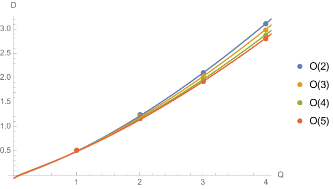
Figure 2: $D(Q)$ from MC simulations in $O(n)$, $n=2,\dots,5$ [10]. The continuous lines are one-parameter fits for the formula in Eq. (5.16) with $\alpha_{3/2}=0.34,\,0.32,\,0.30,\,0.29$.

The action in Eq. (5.4) is not the most general one compatible with the symmetries of the problem. In fact, in terms of the fields $\phi_{2k-1}$ and $\phi_{2k}$, we could have started with $1/2\pqty{\mathop{\mathrm{{}\partial}}\mathopen{}_{\mu}\phi_{2k-1}}^{2}+b/2\phi_{2k-1}^{2}\pqty{\mathop{\mathrm{{}\partial}}\mathopen{}_{\mu}\phi_{2k}}^{2}$, where $b$ is an arbitrary parameter. In the spirit of [1], this gives the effective Wilsonian action describing the conformal fixed point of the $O(n)$ model in the limit of large charge. Repeating the computations we find that the coefficients $\alpha_{3/2}$ and $\alpha_{1/2}$ are independent and their product is $\alpha_{3/2}\alpha_{1/2}=1/(12b)$. Interestingly enough, though, fitting the values for the conformal dimensions stemming from MC simulations, shows that empirically the product $\alpha_{3/2}\alpha_{1/2}$ is compatible with the value $b=1$ that we used above. We intend to revisit the question of this apparent coincidence in future work.

References

• [1] Simeon Hellerman, Domenico Orlando, Susanne Reffert and Masataka Watanabe “On the CFT Operator Spectrum at Large Global Charge” In JHEP 12, 2015, pp. 071 DOI: 10.1007/JHEP12(2015)071
• [2] G. S. Guralnik, C. R. Hagen and T. W. B. Kibble “Broken symmetries and the Goldstone theorem” In ’Advances in Particle Physics’, R.L. Cool and R.E. Marshak (Eds.), Vol. 2, pp. 567-708, 1968, New York: Interscience Publishers, 1968
• [3] Holger Bech Nielsen and S. Chadha “On How to Count Goldstone Bosons” In Nucl. Phys. B105, 1976, pp. 445–453 DOI: 10.1016/0550-3213(76)90025-0
• [4] Tomas Brauner “Spontaneous Symmetry Breaking and Nambu-Goldstone Bosons in Quantum Many-Body Systems” In Symmetry 2, 2010, pp. 609–657 DOI: 10.3390/sym2020609
• [5] Haruki Watanabe, Tomáš Brauner and Hitoshi Murayama “Massive Nambu-Goldstone Bosons” In Phys. Rev. Lett. 111.2, 2013, pp. 021601 DOI: 10.1103/PhysRevLett.111.021601
• [6] Thomas Schäfer et al. “Kaon condensation and Goldstone’s theorem” In Phys. Lett. B522, 2001, pp. 67–75 DOI: 10.1016/S0370-2693(01)01265-5
• [7] Alberto Nicolis and Federico Piazza “Spontaneous Symmetry Probing” In JHEP 06, 2012, pp. 025 DOI: 10.1007/JHEP06(2012)025
• [8] Alberto Nicolis and Federico Piazza “Implications of Relativity on Nonrelativistic Goldstone Theorems: Gapped Excitations at Finite Charge Density” [Addendum: Phys. Rev. Lett.110,039901(2013)] In Phys. Rev. Lett. 110.1, 2013, pp. 011602 DOI: 10.1103/PhysRevLett.110.011602, 10.1103/PhysRevLett.110.039901
• [9] Alberto Nicolis, Riccardo Penco, Federico Piazza and Rachel A. Rosen “More on gapped Goldstones at finite density: More gapped Goldstones” In JHEP 11, 2013, pp. 055 DOI: 10.1007/JHEP11(2013)055
• [10] Martin Hasenbusch and Ettore Vicari “Anisotropic perturbations in three-dimensional $O(N)$-symmetric vector models” In Phys. Rev. B 84, 2011, pp. 125136 arXiv:1108.0491 [cond-mat]
• [11] Filip Kos, David Poland, David Simmons-Duffin and Alessandro Vichi “Bootstrapping the O(N) Archipelago” In JHEP 11, 2015, pp. 106 DOI: 10.1007/JHEP11(2015)106
• [12] Yu Nakayama and Tomoki Ohtsuki “Conformal Bootstrap Dashing Hopes of Emergent Symmetry” In Phys. Rev. Lett. 117.13, 2016, pp. 131601 DOI: 10.1103/PhysRevLett.117.131601
• [13] Ming-wen Xiao “Theory of transformation for the diagonalization of quadratic Hamiltonians”, 2009 URL: http://cds.cern.ch/record/1198089
• [14] A. Monin “Partition function on spheres: How to use zeta function regularization” In Phys. Rev. D94.8, 2016, pp. 085013 DOI: 10.1103/PhysRevD.94.085013