Fictitious domain method with boundary value correction using penalty-free Nitsche method

Abstract

In this paper, we consider a fictitious domain approach based on a Nitsche type method without penalty. To allow for high order approximation using piecewise affine approximation of the geometry we use a boundary value correction technique based on Taylor expansion from the approximate to the physical boundary. To ensure stability of the method a ghost penalty stabilization is considered in the boundary zone. We prove optimal error estimates in the $H^{1}$-norm and estimates suboptimal by $\mathcal{O}(h^{\frac{1}{2}})$ in the $L^{2}$-norm. The suboptimality is due to the lack of adjoint consistency of our formulation. Numerical results are provided to corroborate the theoretical study.

Boundary value correction, penalty-free Nitsche method Boiveau Thomas T. Boiveau Department of Mathematics, University College London, Gower Street, London, UK-WC1E 6BT United Kingdom thomas.boiveau.12@ucl.ac.uk Burman Erik E. Burman Department of Mathematics, University College London, Gower Street, London, UK-WC1E 6BT United Kingdom Claus Susanne S, Claus Cardiff School of Engineering, Cardiff University, Queen’s Buildings, The Parade, Cardiff CF24 3AA, Wales United Kingdom Larson Mats G. M. G. Larson Department of Mathematics and Mathematical Statistics, Umeå University, SE-90187 Umeå Sweden This work received funding from EPSRC (award number EP/J002313/1) which is gratefully acknowledged. The Author, S. Claus, gratefully acknowledges the financial support provided by the Welsh Government and Higher Education Funding Council for Wales through the S r Cymru National Research Network in Advanced Engineering and Materials. The author M. G. Larson gratefully acknowledges the financial support from the Swedish Foundation for Strategic Research Grant No. AM13-0029, the Swedish Research Council Grant No. 2011-4992, and Swedish strategic research programme eSSENCE.

1 Introduction

Mesh generation is an important challenge in computational mechanics, in fact for complex geometries this can be highly nontrivial. In some cases for time dependent problems, such as a solid body embedded in a flow, the geometry of the problem changes each time step imposing conintuous remeshing, at least locally. The main idea of the fictitious domain method [11, 12, 13, 1, 14, 7, 8, 18] is to relax the constraint that imposes the mesh to fit with the computational domain. In fact the principle is to embed the computational domain in a mesh that is easy to generate, without matching the elements with the boundary. In the early developments of fictitious domain [11], the method was faced with the choice of either integrating the equations over the whole computational mesh including the nonphysical part or only integrate inside the physical domain. In the first case, the method is robust but inaccurate, the second approach is accurate but can generate bad conditioning of the system matrix depending on how the boundary crosses the mesh. As a fix to solve the conditioning problem a boundary penalty term was introduced in [3] the effect of this term is that it extends the stability in the physical domain to the whole mesh domain, provided the distance from the mesh boundary to the physical boundary is $\mathcal{O}(h)$.

Nitsche’s method was first introduced for the weak imposition of the boundary conditions in [19] and designed to be consistent and preserve the symmetry of the original problem. The stability of the method relies on a penalty term that needs to be sufficiently large. In the context of fictitious domain methods Nitsche’s method can suffer from instability for certain mesh boundary configurations. A solution to this problem using the ghost penalty approach was suggested in [8, 18].

In [10] a non-symmetric version was proposed where the penalty parameter only needs to be strictly greater than zero for the stability to be ensured. The possibility of considering the penalty parameter equal to zero for the non-symmetric case was suggested in [15], however, coercivity cannot be proved for this non-symmetric penalty-free method and stability was not established. In [4] the stability of the nonsymmetric Nitsche’s method without penalty for elliptic problems was proved, using an inf-sup argument, drawing on earlier work on discontinuous Galerkin methods [16]. Recently the work on penalty free methods has been extended to compressible and incompressible elasticity in [2]. The penalty-free method can be seen as a Lagrange multiplier method where the Lagrange multipliers has been replaced by the the boundary fluxes of the discrete elliptic operator. In multiphysics problems and particularly for fluid-structure interaction the loose coupling of this method appears to have some advantages that has been observed numerically in [6].

We consider a cut finite element method (CutFEM) [5] in the fictitious domain fashion, the implementation of this method often requires an approximation of the physical domain due to the boundary that can arbitrarily cut through the elements of the mesh. In this paper we propose a method to control the error introduced by this approximation of the physical domain. We follow the method that has been developed in [9] where a piecewise affine approximate geometry was used for the integration of the equation with a correction based on Taylor expansion from the approximate to the physical boundary to improve order when higher polynomial orders are used. In this work we use the penalty-free Nitsche’s method to impose the boundary conditions. This eliminates one penalty parameter at the price of loss of symmetry of the algebraic system and $\mathcal{O}(h^{\frac{1}{2}})$ suboptimality in the $L^{2}$-norm. We believe that the method nevertheless may be of interest, in particular for problems that are not symmetric, such as the advection–diffusion equation. We present and analyse the method in the two-dimensional case, but the results hold also in the three dimensional case.

We end this section by introducing our model problem. Let $\Omega$ be a bounded domain in $\mathbb{R}^{2}$ with smooth boundary $\Gamma$ and exterior unit normal $n$. The Poisson problem is given by:

$$-\Delta u =f\quad\text{in}~{}\Omega,$$

$$u =g\quad\text{on}~{}\Gamma,$$

where $f\in L^{2}(\Omega)$ the given body force and $g\in H^{\frac{3}{2}}(\Omega)$ the boundary condition. The following regularity estimate holds

$$\|u\|_{H^{s+2}(\Omega)}\lesssim\|f\|_{H^{s}(\Omega)}~{}~{}~{},~{}~{}~{}~{}~{}~{}s\geq-1.$$ (1)

In this paper $C$ will be used as a generic positive constant that may change at each occurrence, we use the notation $a\lesssim b$ for $a\leq Cb$. We will also use $a\sim b$ to denote $a\lesssim b$ and $b\lesssim a$.

2 Preliminaries

Let $\left\{\mathcal{T}_{h}\right\}_{h}$ be a family of quasi-uniform and shape regular triangulations. In a generic sense a node of the triangulation is designated by $x_{i}$, $K$ denotes a triangle of $\mathcal{T}_{h}$ and $F$ denotes a face of a triangle $K$. $h_{K}=\mbox{diam}(K)$ is the diameter of $K$ and $h=\mbox{max}_{K\in\mathcal{T}_{h}}h_{K}$ the mesh parameter for a given triangulation $\mathcal{T}_{h}$. $\mathbb{P}_{p}(K)$ defines the space of polynomials of degree less than or equal to $p$ on the element $K$, $\Omega_{\mathcal{T}}$ is the domain covered by the mesh $\mathcal{T}_{h}$, let us introduce the following finite element space

$$V_{h}^{p}=\left\{v\in H^{1}(\Omega_{\mathcal{T}}):v|_{K}\in\mathbb{P}_{p}(K)~{}~{}\forall K\in\mathcal{T}_{h}\right\}.$$

For simplicity we will write the $L^{2}$-norm on a domain $\Theta$, $\|\cdot\|_{L^{2}(\Theta)}$ as $\|\cdot\|_{\Theta}$. The domain $\Omega$ is embedded in a mesh $\mathcal{T}_{h}$. Figure 1 gives an example of a simple configuration.

Figure 1: Domain $\Omega$ embedded in a background mesh $\mathcal{T}_{h}$.

We define $\rho$ as the signed distance function, negative on the inside and positive on the outside of $\Omega$. The tubular neighbourhood of $\Gamma$ is defined as $U_{\delta}(\Gamma)=\{x\in\mathbb{R}^{2}:|\rho(x)|<\delta\}$. We consider a constant $\delta_{0}>0$ such that the closest point mapping $p(x):U_{\delta_{0}}(\Gamma)\rightarrow\Gamma$ is well defined and we have the identity $p(x)=x-\rho(x)n(p(x))$. We suppose that $\delta_{0}$ is chosen small enough such that $p(x)$ is a bijection. Let the polygonal domain $\Omega_{h}$ with boundary $\Gamma_{h}$, be a domain approximating $\Omega$. For simplicity we will assume that the discrete domain is defined by the zero levelset of the nodal interpolant of $\rho$ on $V_{h}^{1}$. Then on a triangle $K$ cut by the boundary, $\Gamma_{h}$ restricted to $K$ is a straight line. The discrete normal $n_{h}$ denotes the exterior unit normal to $\Gamma_{h}$. Observe that $n_{h}$ is constant on $\Gamma_{h}|_{K}$. We define $p_{h}(x,\varsigma)=x+\varsigma n_{h}(x)$, the function $\varrho_{h}$ is defined by $\varrho_{h}:\Gamma_{h}\longrightarrow\mathbb{R}$ such that $p_{h}(x,\varrho_{h}(x))\in\Gamma$ for all $x\in\Gamma_{h}$, for simplicity let $p_{h}(x)=p_{h}(x,\varrho_{h}(x))$. Observe that $\varrho_{h}$ is well defined for $h$ small enough (see [9]). We assume that $p_{h}(x,\varsigma)\in U_{\delta_{0}}(\Omega)$ for all $x\in\Gamma_{h}$ and all $\varsigma$ between $0$ and $\varrho_{h}(x)$. By our definition of $\Omega_{h}$ we have

$$\delta_{h}=\|\varrho_{h}\|_{L^{\infty}(\Gamma_{h})}=\mathcal{O}(h^{2}).$$ (2)

Let $\omega$ be a subset of $\Omega_{\mathcal{T}}$, we define

$$\mathcal{K}_{h}(\omega)=\left\{K\in\mathcal{T}_{h}~{}|~{}\overline{K}\cap\overline{\omega}\neq\emptyset\right\},\quad\quad\mathcal{N}_{h}(\omega)=\cup_{K\in\mathcal{K}_{h}(\omega)}K,$$

and the norm

$$\|v\|_{\mathcal{N}_{h}(\omega)}=\left(\sum_{K\in\mathcal{K}_{h}(\omega)}\|v\|_{K}^{2}\right)^{\frac{1}{2}}.$$

We will use the notations

$$\mathcal{K}_{h} =\mathcal{K}_{h}(\Omega\cup\Omega_{h}),$$

$$\mathcal{K}_{\Gamma} =\mathcal{K}_{h}(\Gamma)\cup\mathcal{K}_{h}(\Gamma_{h}),$$

$$\mathcal{N}_{h} =\mathcal{N}_{h}(\Omega\cup\Omega_{h}).$$

We now recall the following trace inequalities for $v\in H^{1}(\mathcal{N}_{h})$

$$\|v\|_{\partial K} \lesssim(h_{K}^{-\frac{1}{2}}\|v\|_{K}+h_{K}^{\frac{1}{2}}\|\nabla v\|_{K})~{}~{}~{}~{}~{}\forall K\in\mathcal{K}_{h},$$ (3)

$$\|v\|_{K\cap\Gamma} \lesssim(h_{K}^{-\frac{1}{2}}\|v\|_{K}+h_{K}^{\frac{1}{2}}\|\nabla v\|_{K})~{}~{}~{}~{}~{}\forall K\in\mathcal{K}_{h}.$$ (4)

Inequality (4) has been shown in [13], we note that this is also true if we consider $\Gamma_{h}$ instead of $\Gamma$. For $v_{h}\in V_{h}^{p}$ the following inverse estimate holds

$$\|\nabla v_{h}\|_{K}\lesssim h_{K}^{-1}\|v_{h}\|_{K}~{}~{}~{}~{}~{}\forall K\in\mathcal{K}_{h}.$$ (5)

The following inequality has been shown in [9] for all $v\in H^{1}(\Omega_{h})$

$$\|v\|_{\Omega_{h}\backslash\Omega}^{2}\lesssim\delta_{h}^{2}\|\nabla v\cdot n\|_{\Omega_{h}\backslash\Omega}^{2}+\delta_{h}\|v\|_{\Gamma_{h}}^{2}.$$ (6)

The ghost penalty [3] is introduced to ensure the well conditioning of the system matrix, it also provides the control of the gradient in case of small cut elements

$$J_{h}(u_{h},v_{h})=\gamma_{g}\sum_{F\in\mathcal{F}_{G}}\sum_{l=1}^{p}h^{2l-1}\langle\llbracket D_{n_{F}}^{l}u_{h}\rrbracket_{F},\llbracket D_{n_{F}}^{l}v_{h}\rrbracket_{F}\rangle_{F},$$

with $\mathcal{F}_{G}=\left\{F\in\mathcal{K}_{\Gamma}~{}|~{}F\cap(\Omega\cup\Omega_{h})\neq\emptyset\right\},$ $\gamma_{g}$ the ghost penalty parameter and $n_{F}$ the unit normal to the face $F$ with fixed but arbitrary orientation. $D^{l}_{n_{F}}$ is the partial derivative of order $l$ in the direction $n_{F}$ and $\llbracket w\rrbracket_{F}=w_{F}^{+}-w_{F}^{-}$, with $w_{F}^{\pm}=\text{lim}_{s\rightarrow 0^{+}}w(x\mp sn_{F})$ is the jump across a face $F$. The following estimate has been shown in [18] for all $v_{h}\in V_{h}^{p}$

$$\|\nabla v_{h}\|_{\mathcal{N}_{h}}^{2}\lesssim\|\nabla v_{h}\|_{\Omega_{h}}^{2}+J_{h}(v_{h},v_{h})\lesssim\|\nabla v_{h}\|_{\mathcal{N}_{h}}^{2}.$$ (7)

We now construct an interpolation operator $\pi_{h}$. Let $\mathbb{E}$ be an $H^{s}$-extension on $\mathcal{N}_{h}$, $\mathbb{E}:H^{s}(\Omega)\rightarrow H^{s}(\mathcal{N}_{h})$ such that for all $w\in$ $(\mathbb{E}w)|_{\Omega}=w$ and

$$\|\mathbb{E}w\|_{H^{s}(\mathcal{N}_{h})}\lesssim\|w\|_{H^{s}(\Omega)}\quad\quad\forall w\in H^{s}(\Omega),s\geq 0.$$ (8)

For simplicity we will write $w$ instead of $\mathbb{E}w$. Let $\pi_{h}^{*}:H^{s}(\mathcal{N}_{h})\rightarrow V_{h}^{p}$ be the Lagrange interpolant, we construct the interpolation operator $\pi_{h}$ such that

$$\pi_{h}u=\pi_{h}^{*}\mathbb{E}u.$$ (9)

We have the interpolation estimate for $0\leq r\leq s\leq p+1$,

$$\|u-\pi_{h}^{*}u\|_{H^{r}(K)}\lesssim h^{s-r}\left|u\right|_{H^{s}(K)}~{}~{}~{}~{}~{}~{}~{}~{}~{}\forall K\in\mathcal{K}_{h}.$$ (10)

Using the estimate (8) together with (10) we have

$$\|u-\pi_{h}u\|_{H^{r}(\mathcal{N}_{h})}\lesssim h^{s-r}\left|u\right|_{H^{s}(\Omega)}.$$ (11)

Let us introduce the norms

$$\vvvert w\vvvert_{h}^{2} =\|\nabla w\|_{\Omega_{h}}^{2}+h^{-1}\|w\|_{\Gamma_{h}}^{2}+J_{h}(w,w),$$

$$\|w\|_{*}^{2} =\vvvert w\vvvert_{h}^{2}+h\|\nabla w\cdot n_{h}\|_{\Gamma_{h}}^{2}+h^{-1}\|T_{1,k}(w)\|_{\Gamma_{h}}^{2},$$

with the Taylor expansion defined such that

$$T_{m,k}(u)(x)=\sum_{i=m}^{k}\frac{D_{n_{h}}^{i}u(x)}{i!}\varrho_{h}^{i}(x),$$ (12)

$D_{n_{h}}^{i}$ is the derivative of order $i$ in the direction $n_{h}$. Using the estimate (11) combined with the trace inequality (3) it is straightforward to show

$$\vvvert u-\pi_{h}u\vvvert_{h}\leq\|u-\pi_{h}u\|_{*}\lesssim h^{p}\left|u\right|_{H^{p+1}(\Omega)}.$$ (13)

3 Finite element formulation

Here we use the boundary value correction approach from [9], we write the extensions of $f$ and $u$ respectively as $f=\mathbb{E}f$ and $u=\mathbb{E}u$.

$$(f,v)_{\Omega_{h}} =(f+\Delta u,v)_{\Omega_{h}}-(\Delta u,v)_{\Omega_{h}}$$

$$=(f+\Delta u,v)_{\Omega_{h}\backslash\Omega}+(\nabla u,\nabla v)_{\Omega_{h}}-\langle\nabla u\cdot n_{h},v\rangle_{\Gamma_{h}}.$$

We know that $f+\Delta u=0$ on $\Omega$. On $\Omega_{h}\backslash\Omega$ we have $f+\Delta u=\mathbb{E}f+\Delta\mathbb{E}u\neq 0$. Let us enforce weakly the boundary condition $u=g$ on $\Gamma$ by adding a consistent boundary term

$$(f,v)_{\Omega_{h}}=(f+\Delta u,v)_{\Omega_{h}\backslash\Omega}+(\nabla u,\nabla v)_{\Omega_{h}}- \langle\nabla u\cdot n_{h},v\rangle_{\Gamma_{h}}$$

$$+\langle\nabla v\cdot n_{h},u\circ p_{h}-g\circ p_{h}\rangle_{\Gamma_{h}}.$$

Remark that this is equivalent to the penalty-free Nitsche’s method [4, 2]. However, we cannot access $u\circ p_{h}$, so we use a Taylor approximation in the direction $n_{h}$ (12)

$$u\circ p_{h}(x)\approx T_{0,k}(u)(x).$$ (14)

We note that in (12) we could replace $n_{h}$ by $n\circ p$ and $\varrho_{h}$ by $\varrho$ if these quantities were available (as mentioned in [9]). Adding and subtracting the Taylor expansion in the Nitsche antisymmetric term and rearranging we obtain

$$\begin{split}(\nabla u,\nabla v)_{\Omega_{h}}&-\langle\nabla u\cdot n_{h},v\rangle_{\Gamma_{h}}+\langle\nabla v\cdot n_{h},T_{0,k}(u)\rangle_{\Gamma_{h}}+(f+\Delta u,v)_{\Omega_{h}\backslash\Omega}\\ &+\langle\nabla v\cdot n_{h},u\circ p_{h}-T_{0,k}(u)\rangle_{\Gamma_{h}}=(f,v)_{\Omega_{h}}+\langle\nabla v\cdot n_{h},g\circ p_{h}\rangle_{\Gamma_{h}}.\end{split}$$ (15)

The discrete formulation is obtained by dropping the terms $(f+\Delta u,v)_{\Omega_{h}\backslash\Omega}$ and $\langle\nabla v\cdot n_{h},u\circ p_{h}-T_{0,k}(u)\rangle_{\Gamma_{h}}$. Find $u_{h}\in V_{h}^{p}$

$$A_{h}(u_{h},v_{h})+J_{h}(u_{h},v_{h})=L_{h}(v_{h})~{}~{}~{}~{}~{}~{}\forall v_{h}\in V_{h}^{p},$$ (16)

with the linear forms

$$A_{h}(u_{h},v_{h}) =(\nabla u_{h},\nabla v_{h})_{\Omega_{h}}-\langle\nabla u_{h}\cdot n_{h},v_{h}\rangle_{\Gamma_{h}}+\langle\nabla v_{h}\cdot n_{h},T_{0,k}(u_{h})\rangle_{\Gamma_{h}},$$

$$L_{h}(v_{h}) =(f,v_{h})_{\Omega_{h}}+\langle\nabla v_{h}\cdot n_{h},g\circ p_{h}\rangle_{\Gamma_{h}}.$$

Using the definition of the Taylor expansion, the bilinear form $A_{h}$ can be written as

$$A_{h}(u_{h},v_{h})=(\nabla u_{h},\nabla v_{h})_{\Omega_{h}}-\langle\nabla u_{h}\cdot n_{h},v_{h}\rangle_{\Gamma_{h}}+ \langle\nabla v_{h}\cdot n_{h},u_{h}\rangle_{\Gamma_{h}}$$

$$+\langle\nabla v_{h}\cdot n_{h},T_{1,k}(u_{h})\rangle_{\Gamma_{h}}.$$

The terms that has been dropped in the discrete formulation are defined as

$$B_{h}(u,v_{h})=(f+\Delta u,v_{h})_{\Omega_{h}\backslash\Omega}+\langle\nabla v_{h}\cdot n_{h},u\circ p_{h}-T_{0,k}(u)\rangle_{\Gamma_{h}}\quad\forall v_{h}\in V_{h}^{p}.$$

In Section 4 we show an inf-sup condition for the discrete formulation (16). In Section 5 the high order terms of $B_{h}(u,v_{h})$ are treated. Section 6 presents the error estimates.

4 Inf-sup condition on $\Omega_{h}$

We assume that $\Omega_{h}$ is defined by the zero level set of the nodal interpolant $\mathcal{I}_{h}\rho$ of the distance function $\rho$. We also assume that $h$ is small enough so that a band of elements in $\mathcal{K}_{h}(\Gamma_{h})$ is in the tubular $U_{\delta_{0}}(\Gamma)$ and that in every $K\in\mathcal{K}_{h}(\Gamma_{h})$ there holds

$$\|\rho-\mathcal{I}_{h}\rho\|_{L^{\infty}(K)}+h\|\nabla(\rho-\mathcal{I}_{h}\rho)\|_{L^{\infty}(K)}\leq c_{\rho}h$$

where the constant $c_{\rho}$ only depends on the regularity of the interface and, since $\rho$ is a distance function, for $x\in\mathcal{K}_{h}(\Gamma_{h})$ we have

$$1\leq|\nabla\rho(x)|\leq C_{1},$$ (17)

with $C_{1}>1$ a constant of order $1$. We now introduce boundary patches that will be useful for the upcoming inf-sup analysis. Let us consider the set $\mathcal{K}_{h}(\Gamma_{h})$ and split it into $N_{p}$ smaller disjoint sets of elements $\mathcal{K}_{j}$ with $j=1,\dots,N_{p}$, then we define

$$P_{j}=\mathcal{K}_{j}\cup\{K\in\mathcal{T}_{h}:K\cap\Omega_{h}\neq\emptyset,\exists K^{\prime}\in\mathcal{K}_{j}\mbox{ such that }K\cap K^{\prime}\neq\emptyset\}.$$

This means that $P_{j}$ consists of the elements on $\mathcal{K}_{j}$ and its neighbours that intersect $\Omega_{h}$ (we assume here that the mesh is truncated beyond $\mathcal{K}_{h}(\Gamma_{h})$ so that there are no exterior neighbours, otherwise it is straightforward to handle them separately). Observe that the patches $P_{j}$ overlap. For each patch $P_{j}$ we define the faces $F_{j}^{1}$ and $F_{j}^{2}$ where $\partial P_{j}\cap\Gamma_{h}\neq\emptyset$. We define the interior elements of the patch by

$$\mathcal{K}_{j}^{\circ}:=\{K\in\mathcal{K}_{h}(\Gamma_{h})\cap P_{j}:K\cap(F_{j}^{1}\cup F_{j}^{2})=\emptyset\}.$$

Let $I_{P_{j}}$ be the set of vertices $\{x_{i}\}$ in the patch $P_{j}$ and the cardinality of $I_{P_{j}}$ is $N_{P_{j}}$. We define the set of mesh vertices $I_{j}$ that are in the interior of the patch $P_{j}$ or on the outer boundary,

$$I_{j}=\left\{x_{i}\in K:K\in\mathcal{K}_{j}^{\circ}\right\},$$

Figure 2 shows an example of a patch. Let $\Gamma_{j}=\Gamma_{h}\cap\mathcal{K}_{j}$ denote the part of the boundary included in the patch $P_{j}$, for all $j$, the patch $P_{j}$ has the following properties

$$\mbox{meas}_{1}(\Gamma_{j})\sim h~{}~{}~{}~{}\text{and}~{}~{}~{}~{}\mbox{meas}_{2}(P_{j})\sim h^{2}.$$ (18)

In (18) we can control the constant in both relations by choosing the patches to contain more elements (but uniformly under refinement).

The function $v_{\Gamma}$ is defined such that $v_{\Gamma}=\sum_{j=1}^{N_{p}}v_{j}$, for each patch $P_{j}$, the function $v_{j}$ has the form $v_{j}=\zeta\tilde{\varphi}_{j}$ with $\zeta\in\mathbb{R}$. Let $\tilde{\varphi}_{j}\in V_{h}^{1}$ be defined for each node $x_{i}\in\mathcal{T}_{h}$ such that

$$\tilde{\varphi}_{j}(x_{i})=\left\{\begin{array}[]{rllr}0&\text{for}&x_{i}\in I_{P_{j}}\setminus I_{j}\\ -\rho(x_{i})&\text{for}&x_{i}\in I_{j},\end{array}\right.$$

with $i=1,\dots,N_{P_{j}}$.

Figure 2: Example of a patch $P_{j}$, in this case $K_{3}\cup K_{4}\cup K_{5}=\mathcal{K}_{j}=\mathcal{K}_{j}^{\circ}$, $\tilde{\varphi}_{j}$ is equal to zero on the nonfilled nodes.

By the Poincaré inequality on a patch $P_{j}$ the following inequality holds

$$\|v_{j}\|_{P_{j}}\lesssim h\|\nabla v_{j}\|_{P_{j}}.$$ (19)

Lemma 4.1.

For every patch $P_{j}$ with $1\leq j\leq N_{p}$ ; $\forall r_{j}\in\mathbb{R}$ there exists $v_{j}\in V_{h}^{p}$ such that

$$\textup{meas}(\Gamma_{j})^{-1}\int_{\Gamma_{j}}\nabla v_{j}\cdot n_{h}~{}\textup{d}s=r_{j},$$ (20)

and the following property holds

$$\|\nabla v_{j}\|_{P_{j}}\lesssim\|h^{\frac{1}{2}}r_{j}\|_{\Gamma_{j}}.$$ (21)

Proof 4.2.

The functions $v_{j}$ and $\tilde{\varphi}_{j}$ are defined as previously described, let

$$\Xi_{j}=\text{meas}(\Gamma_{j})^{-1}\int_{\Gamma_{j}}\nabla\tilde{\varphi}_{j}\cdot n_{h}~{}\text{d}s.$$

We will first prove that for shape regular meshes, $\Xi_{j}$ is strictly negative and bounded away from zero uniformly in $h$, provided the hidden constant of the upper bound in (18) is chosen large enough. Let $K_{1},\dots,K_{m}$ be the triangles crossed by $\Gamma_{h}$ within a patch $P_{j}$, the numbering of the crossed elements is done in order following a path of $\Gamma_{j}$ as in figure 2. The assumption (18) says that the number of these triangles should be uniformly bounded by some $m$. We will show that the upper bound $m$ only depends on the shape regularity of the mesh. The mesh size on the other hand must be small enough to resolve the boundary. The triangles $K_{1}$, $K_{2}$, $K_{m-1}$ and $K_{m}$ will have nodes on the boundary of $\partial P_{i}$ where $\tilde{\varphi}=0$ (on $F_{j}^{1}$ or $F_{j}^{2}$). Let us merge $K_{1}$ and $K_{2}$ (resp. $K_{m-1}$ and $K_{m}$) into one quadrilateral element $K_{1}^{\square}$ (resp. $K_{m}^{\square}$). Observe that for the triangles $K_{i}$, $i=3,...,m-2$ there holds $K_{i}\in\mathcal{K}_{j}^{\circ}$ and with $\mathcal{I}_{h}$ denoting the standard nodal interpolant on piecewise linear functions,

$$(n_{h}\cdot\nabla\tilde{\varphi}_{j}|_{K_{i}})=|\nabla\mathcal{I}_{h}\rho|_{K_{i}}|.$$

On $K_{1}^{\square}$ and $K_{m}^{\square}$ the following upper bound holds trivially

$$(n_{h}\cdot\nabla\tilde{\varphi}_{j}|_{K_{i}^{\square}})<|\nabla\tilde{\varphi}_{j}|_{K_{i}^{\square}}|,\quad i=1,m.$$

Consider now

$$\int_{\Gamma_{h}\cap P_{j}}\nabla\tilde{\varphi}_{j}\cdot n_{h}~{}\text{d}s=\sum_{i=1}^{m}\int_{\Gamma_{j}\cap K_{i}}\nabla\tilde{\varphi}_{j}\cdot n_{h}~{}\text{d}s=T_{1}^{\square}+T_{m}^{\square}+\sum_{i=3}^{m-2}T_{i}.$$

For $i\in\{3,\ldots,m-2\}$ using (17) we have

$$T_{i}=|\nabla\pi_{h}\rho|_{K_{i}}|\mbox{meas}(\Gamma_{j}\cap K_{i})\geq\mbox{meas}(\Gamma_{j}\cap K_{i})(1-|\nabla(1-\mathcal{I}_{h})\rho|_{K_{i}}|)\\ \geq(1-c_{\rho}h)\mbox{meas}(\Gamma_{j}\cap K_{i}).$$

For $i\in\{1,m\}$ we have

$$T_{i}^{\square}\leq h^{\frac{1}{2}}\|\nabla\tilde{\varphi}_{j}\|_{F_{j}\cap K_{i}^{\square}}\leq\|\nabla\tilde{\varphi}_{j}\|_{K_{i}^{\square}}\leq C_{i}h^{-1}\|\tilde{\varphi}_{j}\|_{K_{i}^{\square}}\leq C_{i}h^{-1/2}\|\mathcal{I}_{h}\rho\|_{\partial K_{i}^{\square}\cap\partial\mathcal{K}_{j}^{\circ}}\\ \leq C_{i}h^{-1/2}(\|\rho\|_{\partial K_{i}^{\square}\cap\partial\mathcal{K}_{j}^{\circ}}+\|\rho-\mathcal{I}_{h}\rho\|_{\partial K_{i}^{\square}\cap\partial\mathcal{K}_{j}^{\circ}})\leq c_{\partial}h.$$

The right hand side of these two inequalities depend only on the shape regularity of the mesh. Hence, using that $\mbox{meas}(\Gamma\cap\mathcal{K}_{j}^{\circ})\geq\mbox{meas}(\Gamma_{j})-2h$

$$\mbox{meas}(\Gamma_{j})^{-1}\sum_{i=1}^{m}\int_{\Gamma_{j}\cap K_{i}}\nabla\tilde{\varphi}_{j}\cdot n_{h}~{}\text{d}s\\ \geq(1-c_{\rho}h)(1-2h\mbox{meas}(\Gamma_{j})^{-1})-2c_{\partial}h\mbox{meas}(\Gamma_{j})^{-1}.$$

Assume now that $h$ is sufficiently small so that $(1-c_{\rho}h)>\frac{1}{2}$ then

$$\mbox{meas}(\Gamma_{j})^{-1}\sum_{i=1}^{m}\int_{\Gamma_{j}\cap K_{i}}\nabla\tilde{\varphi}_{j}\cdot n_{h}~{}\text{d}s\geq\frac{1}{2}-(2c_{\partial}+1)h\mbox{meas}(\Gamma_{j})^{-1}.$$

If the lower constant of the left relation of (18) is larger than $4(2c_{\partial}+1)$ we may conclude that

$$\Xi_{j}=\mbox{meas}(\Gamma_{j})^{-1}\sum_{i=1}^{m}\int_{\Gamma_{j}\cap K_{i}}\nabla\tilde{\varphi}_{j}\cdot n_{h}~{}\text{d}s\geq\frac{1}{4},$$

which shows the uniform lower bound. Note that the constant $c_{\partial}$ only depends on the curvature of the boundary and the mesh geometry. Thanks to this lower bound we may define the normalised function $\varphi_{j}$ by

$$\varphi_{j}=\Xi_{j}^{-1}\tilde{\varphi}_{j}.$$

By definition there holds

$$\textup{meas}(\Gamma_{j})^{-1}\int_{\Gamma_{j}}\nabla\varphi_{j}\cdot n_{h}~{}\textup{d}s=1,$$ (22)

and

$$\|\nabla\varphi_{j}\|_{P_{j}}=\Xi_{j}^{-1}\|\nabla\tilde{\varphi}_{j}\|_{P_{j}}.$$ (23)

The right hand side can be bounded as follows

$$\|\nabla\tilde{\varphi}_{j}\|_{P_{j}}\leq\|\nabla\tilde{\varphi}_{j}\|_{\mathcal{K}_{j}^{\circ}}+\|\nabla\tilde{\varphi}_{j}\|_{P_{j}\setminus\mathcal{K}_{j}^{\circ}}=T_{1}+T_{2},$$

$$T_{1}\leq\|\nabla(\pi_{h}\rho-\rho)\|_{\mathcal{K}_{j}^{\circ}}+\|\nabla\rho\|_{\mathcal{K}_{j}^{\circ}}\leq Ch^{\frac{1}{2}}\mbox{meas}(\Gamma_{j})^{\frac{1}{2}},$$

$$T_{2}\leq C_{i}h^{-1}\|\tilde{\varphi}_{j}\|_{P_{i}\setminus\mathcal{K}_{j}^{\circ}}\leq Ch^{-1/2}\|\mathcal{I}_{h}\rho\|_{\partial\mathcal{K}_{j}^{\circ}}\\ \leq Ch^{-1/2}(\|\rho\|_{\partial\mathcal{K}_{j}^{\circ}}+\|\mathcal{I}_{h}\rho-\rho\|_{\partial\mathcal{K}_{j}^{\circ}})\leq Ch^{\frac{1}{2}}\mbox{meas}(\Gamma_{j})^{\frac{1}{2}}.$$

We conclude that

$$\|\nabla\varphi_{j}\|_{P_{j}}\leq Ch^{\frac{1}{2}}\mbox{meas}(\Gamma_{j}).$$ (24)

Let $v_{j}=r_{j}\varphi_{j}$, then condition (20) is verified considering (22). The upper bound (21) is obtained using (24), (18) and

$$\|\nabla v_{j}\|_{P_{j}}=|r_{j}|\|\nabla\varphi_{j}\|_{P_{j}}\lesssim\text{meas}(\Gamma_{j})^{\frac{1}{2}}|r_{j}|h^{\frac{1}{2}}=\|h^{\frac{1}{2}}r_{j}\|_{\Gamma_{j}}.$$

Lemma 4.3.

For $u_{h},v_{h}\in V_{h}^{p}$ with $v_{h}=u_{h}+\alpha v_{\Gamma}$, there exists a positive constant $\beta_{0}$ such that the following inequality holds

$$\beta_{0}\vvvert u_{h}\vvvert_{h}^{2}\leq A_{h}(u_{h},v_{h})+J_{h}(u_{h},v_{h}).$$

Proof 4.4.

Using (7) it is straightforward to obtain

$$\begin{split}(A_{h}+J_{h})(u_{h},u_{h})=&~{}(\nabla u_{h},\nabla u_{h})_{\Omega_{h}}+\langle\nabla u_{h}\cdot n_{h},T_{1,k}(u_{h})\rangle_{\Gamma_{h}}+J_{h}(u_{h},u_{h})\\ &\gtrsim\|\nabla u_{h}\|_{\mathcal{N}_{h}}^{2}+\langle\nabla u_{h}\cdot n_{h},T_{1,k}(u_{h})\rangle_{\Gamma_{h}}.\end{split}$$

We bound the second term using the trace inequality (4), inverse inequality (5) and (2)

$$\langle\nabla u_{h}\cdot n_{h},T_{1,k}(u_{h})\rangle_{\Gamma_{h}} \leq\|\nabla u_{h}\cdot n_{h}\|_{\Gamma_{h}}\|T_{1,k}(u_{h})\|_{\Gamma_{h}}$$

$$\lesssim h^{-1}\|\nabla u_{h}\|_{\mathcal{N}_{h}(\Gamma_{h})}\|T_{1,k}(u_{h})\|_{\mathcal{N}_{h}(\Gamma_{h})}$$

$$\lesssim\gamma(h)\|\nabla u_{h}\|_{\mathcal{N}_{h}(\Gamma_{h})}^{2},$$

where $\gamma(h)=\sum_{i=1}^{k}\left(\frac{\delta_{h}}{h}\right)^{i}$, note that $\mathcal{O}(\gamma(h))=h$. Considering $v_{\Gamma}$ as defined in Section 2, for the $j^{th}$ patch $P_{j}$ we get

$$\alpha(A_{h}+J_{h})(u_{h},v_{j})=\alpha (\nabla u_{h},\nabla v_{j})_{P_{j}\cap\Omega_{h}}-\alpha\langle\nabla u_{h}\cdot n_{h},v_{j}\rangle_{\Gamma_{j}}+\alpha J_{h}(u_{h},v_{j})$$

$$+\alpha\langle\nabla v_{j}\cdot n_{h},u_{h}\rangle_{\Gamma_{j}}+\alpha\langle\nabla v_{j}\cdot n_{h},T_{1,k}(u_{h})\rangle_{\Gamma_{j}},$$

applying Cauchy-Schwarz inequality together with (7) we can write

$$\alpha(\nabla u_{h} ,\nabla v_{j})_{P_{j}\cap\Omega_{h}}+\alpha J_{h}(u_{h},v_{j})$$

$$\leq\alpha\|\nabla u_{h}\|_{P_{j}\cap\Omega_{h}}\|\nabla v_{j}\|_{P_{j}\cap\Omega_{h}}+\alpha J_{h}(u_{h},u_{h})^{\frac{1}{2}}J_{h}(v_{j},v_{j})^{\frac{1}{2}},$$

$$\leq\epsilon\|\nabla u_{h}\|_{P_{j}}^{2}+\frac{C\alpha^{2}}{4\epsilon}\|\nabla v_{j}\|_{P_{j}}^{2}.$$

Using the trace inequality (4), the inverse inequality (5) and the inequality (19) we can write the following

$$\alpha\langle\nabla u_{h}\cdot n_{h},v_{j}\rangle_{\Gamma_{j}} \leq\alpha\|\nabla u_{h}\cdot n_{h}\|_{\Gamma_{j}}\|v_{j}\|_{\Gamma_{j}}\lesssim\alpha h^{-1}\|\nabla u_{h}\|_{P_{j}}\|v_{j}\|_{P_{j}}$$

$$\lesssim\alpha\|\nabla u_{h}\|_{P_{j}}\|\nabla v_{j}\|_{P_{j}}\leq\epsilon\|\nabla u_{h}\|_{P_{j}}^{2}+\frac{C\alpha^{2}}{4\epsilon}\|\nabla v_{j}\|_{P_{j}}^{2}.$$

Let us consider the average $\overline{u}^{j}=\text{meas}(\Gamma_{j})^{-1}\int_{\Gamma_{j}}u_{h}~{}\text{d}s$. Using Lemma 4.1 and choosing $r_{j}=h^{-1}\overline{u}^{j}$ we get the inequality

$$\|\nabla v_{j}\|_{P_{j}}\lesssim\|h^{-\frac{1}{2}}\overline{u}^{j}\|_{\Gamma_{j}}.$$ (25)

Our choice of $r_{j}$ allows us to write

$$\alpha\langle\nabla v_{j}\cdot n_{h},u_{h}\rangle_{\Gamma_{j}}=\alpha\|h^{-\frac{1}{2}}\overline{u}^{j}\|_{\Gamma_{j}}^{2}+\alpha\langle\nabla v_{j}\cdot n_{h},u_{h}-\overline{u}^{j}\rangle_{\Gamma_{j}}.$$

It is straightforward to observe

$$\|u_{h}-\overline{u}^{j}\|_{\Gamma_{j}}\leq Ch\|\nabla u_{h}\|_{\Gamma_{j}},$$ (26)

combining this result with the trace and inverse inequalities, we can show

$$\alpha\langle\nabla v_{j}\cdot n_{h},u_{h}-\overline{u}^{j}\rangle_{\Gamma_{j}}\leq\epsilon\|\nabla u_{h}\|_{P_{j}}^{2}+\frac{C\alpha^{2}}{4\epsilon}\|\nabla v_{j}\|_{P_{j}}^{2}.$$

Using (2) once again

$$\alpha\langle\nabla v_{j}\cdot n_{h},T_{1,k}(u_{h})\rangle_{\Gamma_{j}}\leq\epsilon\gamma(h)^{2}\|\nabla u_{h}\|_{P_{j}}^{2}+\frac{C\alpha^{2}}{4\epsilon}\|\nabla v_{j}\|_{P_{j}}^{2}.$$

Each term has been bounded, we can now get back to

$$\begin{split}(A_{h}+J_{h})(u_{h},v_{h})\geq(C-\gamma(h))&\|\nabla u_{h}\|_{\mathcal{N}_{h}}^{2}+\alpha\sum_{j=1}^{N_{p}}\|h^{-\frac{1}{2}}\overline{u}^{j}\|_{\Gamma_{j}}^{2}\\ &-4\epsilon\sum_{j=1}^{N_{p}}\|\nabla u_{h}\|_{P_{j}}^{2}-\frac{C\alpha^{2}}{\epsilon}\sum_{j=1}^{N_{p}}\|\nabla v_{j}\|_{P_{j}}^{2},\end{split}$$

using (25) and rearranging, we obtain

$$\begin{split}(A_{h}+J_{h})(u_{h},v_{h})\geq(C-\gamma(h)-4\epsilon)\|\nabla u_{h}\|_{\mathcal{N}_{h}}^{2}+\alpha\Big{(}1-\frac{C\alpha}{\epsilon}\Big{)}\sum_{j=1}^{N_{p}}\|h^{-\frac{1}{2}}\overline{u}^{j}\|_{\Gamma_{j}}^{2}.\end{split}$$

Using (26), the trace inequality and the inverse inequality we can show

$$\|h^{-\frac{1}{2}}\overline{u}^{j}\|_{\Gamma_{j}}^{2}\geq\|h^{-\frac{1}{2}}u_{h}\|_{\Gamma_{j}}^{2}-C^{\prime}\|\nabla u_{h}\|_{P_{j}}^{2},$$

using this result together with (7) we obtain

$$\begin{split}(A_{h}+J_{h})(u_{h},v_{h})\geq&~{}(C-\gamma(h)-4\epsilon-C^{\prime}\alpha)\left(\|\nabla u_{h}\|_{\Omega_{h}}^{2}+J_{h}(u_{h},u_{h})\right)\\ &+\alpha\Big{(}1-\frac{C\alpha}{\epsilon}\Big{)}\sum_{j=1}^{N_{p}}\|h^{-\frac{1}{2}}u_{h}\|_{\Gamma_{j}}^{2}.\end{split}$$

It is easy to choose $\epsilon$ and $\alpha$ such that the two terms of this expression are positive, for example, by choosing $\epsilon=\frac{1}{16}$ we obtain $\alpha=\text{min}(\frac{C-\gamma(h)-\frac{1}{4}}{C^{\prime}},\frac{1}{16C})$.

Theorem 4.5.

There exists a positive constant $\beta$ such that for all function $u_{h}\in V_{h}^{p}$ the following inequality holds

$$\beta\vvvert u_{h}\vvvert_{h}\leq\underset{v_{h}\in V_{h}^{p}}{\textup{sup}}\frac{A_{h}(u_{h},v_{h})+J_{h}(u_{h},v_{h})}{\vvvert v_{h}\vvvert_{h}}.$$

Proof 4.6.

Considering Lemma 4.3 the only thing to show is $\vvvert v_{h}\vvvert_{h}\lesssim\vvvert u_{h}\vvvert_{h}$,

$$\vvvert v_{h}\vvvert_{h}\leq\vvvert u_{h}\vvvert_{h}+\vvvert v_{\Gamma}\vvvert_{h}~{}~{}~{}\text{with}~{}~{}~{}~{}~{}\vvvert v_{\Gamma}\vvvert_{h}\leq\sum_{j=1}^{N_{p}}\vvvert v_{j}\vvvert_{h},$$

$$\vvvert v_{j}\vvvert_{h}^{2}=\|\nabla v_{j}\|_{P_{j}\cap\Omega_{h}}^{2}+\|h^{-\frac{1}{2}}v_{j}\|_{\Gamma_{j}}^{2}+J_{h}(v_{j},v_{j}).$$

Using the trace inequality together with (19) and (25) we observe

$$\|h^{-\frac{1}{2}}v_{j}\|_{\Gamma_{j}}^{2}\lesssim\|\nabla v_{j}\|_{P_{j}}^{2}\lesssim\|h^{-\frac{1}{2}}\overline{u}^{j}\|_{\Gamma_{j}}\lesssim\|h^{-\frac{1}{2}}u_{h}\|_{\Gamma_{j}}.$$

We conclude using (7).

5 Boundary value correction

The goal of this section is bound the two high order terms that has been dropped in the finite element formulation (16).

Theorem 5.1.

Let $B_{h}$ be the bilinear form as defined in (3) the following holds $\forall v_{h}\in V_{h}^{p}$

$$B_{h}(u,v_{h})\lesssim(h^{-\frac{1}{2}}\delta_{h}^{k+1}\underset{0\leq t\leq\delta_{0}}{\textup{sup}}\|D^{k+1}u\|_{\Gamma_{t}}+\delta_{h}^{l+1}\underset{0\leq t\leq\delta_{0}}{\textup{sup}}\|D_{n}^{l}(f+\Delta u)\|_{\Gamma_{t}})\vvvert v_{h}\vvvert_{h}.$$

Proof 5.2.

Using the Cauchy-Schwarz inequality

$$|B_{h}(u,v_{h})|\leq\|u\circ p_{h}(x)-T_{0,k}(u)(x)\|_{\Gamma_{h}}\|\nabla v_{h}\cdot n_{h}\|_{\Gamma_{h}}+\|f+\Delta u\|_{\Omega_{h}\backslash\Omega}\|v_{h}\|_{\Omega_{h}\backslash\Omega}.$$

By definition of the Taylor approximation we have

$$|u\circ p_{h}(x)-T_{0,k}(u)(x)|=\Big{|}\int_{0}^{\varrho_{h}(x)}D_{n_{h}}^{k+1}u(x(s))(\varrho_{h}(x)-s)^{k}~{}\text{d}s\Big{|}.$$

Using the Cauchy Schwarz inequality

$$\|u\circ p_{h}(x)-T_{0,k}(u)(x)\|_{\Gamma_{h}}^{2} \leq\int_{\Gamma_{h}}\|D_{n_{h}}^{k+1}u\|_{I_{x}}^{2}\|(\varrho_{h}(x)-s)^{k}\|_{I_{x}}^{2}~{}\text{d}s$$

$$\leq\int_{\Gamma_{h}}\|D_{n_{h}}^{k+1}u\|_{I_{\delta_{h}}}^{2}|\varrho_{h}(x)|^{2k+1}~{}\text{d}s$$

$$\leq\delta_{h}^{2k+1}\|D^{k+1}u\|_{U_{\delta_{h}}(\Gamma_{h})}^{2}$$

$$\leq\delta_{h}^{2k+2}\underset{0\leq t\leq\delta_{0}}{\text{sup}}\|D^{k+1}u\|_{\Gamma_{t}}^{2},$$

where $\Gamma_{t}=\{x\in\Omega~{}:~{}|\rho(x)|=t\}$ is the levelset with distance $t$ to the boundary $\Gamma$, following the approach from [9]. Suppose that

$$f+\Delta u\in H^{l}(U_{\delta_{0}}(\Omega)),$$

this property holds if $f\in H^{l}(\Omega)$ by applying (1) and (8). Using $\Omega_{h}\backslash\Omega\in U_{\delta}(\Gamma)$ and $\delta\sim\delta_{h}$ it follows that

$$\|f+\Delta u\|_{\Omega_{h}\backslash\Omega}\lesssim\delta_{h}^{l}\|D_{n}^{l}(f+\Delta u)\|_{\Omega_{h}\backslash\Omega}\lesssim\delta_{h}^{l+\frac{1}{2}}\underset{0\leq t\leq\delta_{0}}{\text{sup}}\|D_{n}^{l}(f+\Delta u)\|_{\Gamma_{t}},$$

Then we can bound the bilinear form $B_{h}$, using $\|v\|_{\Omega_{h}\backslash\Omega}\lesssim\delta_{h}^{1/2}\vvvert v\vvvert_{h}$ (deduced from (6)) the trace and inverse inequalities $\forall v_{h}\in V_{h}^{p}$

$$\begin{split}|&B_{h}(u,v_{h})|\\ &\lesssim\delta_{h}^{k+1}\underset{0\leq t\leq\delta_{0}}{\text{sup}}\|D^{k+1}u\|_{\Gamma_{t}}\|\nabla v_{h}\cdot n_{h}\|_{\Gamma_{h}}+\delta_{h}^{l+\frac{1}{2}}\underset{0\leq t\leq\delta_{0}}{\text{sup}}\|D_{n}^{l}(f+\Delta u)\|_{\Gamma_{t}}\|v_{h}\|_{\Omega_{h}\backslash\Omega}\\ &\lesssim(h^{-\frac{1}{2}}\delta_{h}^{k+1}\underset{0\leq t\leq\delta_{0}}{\text{sup}}\|D^{k+1}u\|_{\Gamma_{t}}+\delta_{h}^{l+1}\underset{0\leq t\leq\delta_{0}}{\text{sup}}\|D_{n}^{l}(f+\Delta u)\|_{\Gamma_{t}})\vvvert v_{h}\vvvert_{h}.\end{split}$$ (27)

6 A priori error estimate

The formulation (16) satisfies the following consistency relation (Galerkin orthogonality).

Lemma 6.1.

Let $u_{h}\in V_{h}^{p}$ be the solution of (16) and $u\in H^{2}(\mathcal{N}_{h})$ be the solution of (1), then

$$A_{h}(u-u_{h},v_{h})-J_{h}(u_{h},v_{h})+B_{h}(u,v_{h})=0~{}~{}~{},~{}~{}~{}\forall v_{h}\in V_{h}^{p}.$$

Proof 6.2.

Subtracting (15) and (16) this is straightforward.

Lemma 6.3.

Let $w\in H^{2}(\mathcal{N}_{h})+V_{h}^{p}$ and $v_{h}\in V_{h}^{p}$ there exists a positive constant $M$ such that

$$A_{h}(w,v_{h})\leq M\|w\|_{*}\vvvert v_{h}\vvvert_{h}.$$

Proof 6.4.

Using the Cauchy-Schwarz inequality, trace inequality and inverse inequality we have

$$(\nabla w,\nabla v_{h})_{\Omega_{h}}-\langle\nabla w\cdot n_{h} ,v_{h}\rangle_{\Gamma_{h}}+\langle\nabla v_{h}\cdot n_{h},T_{0,k}(w)\rangle_{\Gamma_{h}}$$

$$\lesssim\|\nabla w\|_{\Omega_{h}}\|\nabla v_{h}\|_{\Omega_{h}}+\|\nabla w\cdot n_{h}\|_{\Gamma_{h}}\|v_{h}\|_{\Gamma_{h}}$$

$$\quad\quad\quad\quad+\|\nabla v_{h}\|_{\Omega_{h}}h^{-1}(\|w\|_{\Gamma_{h}}+\|T_{1,k}(w)\|_{\Gamma_{h}}).$$

Using the inf-sup condition from Section 4 and the estimate obtained in Section 5 the error in the triple norm can now be estimated.

Proposition 6.5.

Let $u\in H^{2}(\mathcal{N}_{h})$ be the solution of (1) and $u_{h}\in V_{h}^{p}$ the solution of (16), then

$$\vvvert u-u_{h}\vvvert_{h}\lesssim h^{p}\|u\|_{H^{p+1}(\Omega)}+h^{-\frac{1}{2}}\delta_{h}^{k+1} \underset{0\leq t\leq\delta_{0}}{\textup{sup}}\|D^{k+1}u\|_{\Gamma_{t}}$$

$$+\delta_{h}^{l+1}\underset{0\leq t\leq\delta_{0}}{\textup{sup}}\|D_{n}^{l}(f+\Delta u)\|_{\Gamma_{t}}.$$

$p$	$h^{p}$	$k$	$h^{-\frac{1}{2}}\delta_{h}^{k+1}$	$l$	$\delta_{h}^{l+1}$
1	$h^{1}$	0	$h^{1.5}$	0	$h^{2}$
2	$h^{2}$	1	$h^{3.5}$	1	$h^{4}$
3	$h^{3}$	2	$h^{5.5}$	2	$h^{6}$
4	$h^{4}$	3	$h^{7.5}$	3	$h^{8}$

Table 1: Order of the terms in the estimation of the $H^{1}$-error depending on $p$, $k$ and $l$, assuming $\delta_{h}=\mathcal{O}(h^{2})$.

Proof 6.6.

Using the Galerkin orthogonality of Lemma 6.1 we obtain

$$A_{h}(u_{h} -\pi_{h}u,v_{h})+J_{h}(u_{h}-\pi_{h}u,v_{h})$$

$$=A_{h}(u-\pi_{h}u,v_{h})-J_{h}(\pi_{h}u,v_{h})+(f+\Delta u,v_{h})_{\Omega_{h}\backslash\Omega}$$

$$\quad\quad\quad\quad\quad\quad\quad\quad\quad\quad\quad+\langle\nabla v_{h}\cdot n_{h},u\circ p_{h}-T_{0,k}(u)\rangle_{\Gamma_{h}}.$$

Using this result, Theorem 4.5, the Lemma 6.3 and $J_{h}(u,v_{h})=0$ given by the regularity of $u$, we can write

$$\beta\vvvert u_{h}- \pi_{h}u\vvvert_{h}\leq\frac{A_{h}(u-\pi_{h}u,v_{h})-J_{h}(\pi_{h}u,v_{h})+B_{h}(u,v_{h})}{\vvvert v_{h}\vvvert_{h}}$$

$$\leq M\|u-\pi_{h}u\|_{*}+\frac{J_{h}(\pi_{h}u-u,\pi_{h}u-u)^{\frac{1}{2}}J_{h}(v_{h},v_{h})^{\frac{1}{2}}+B_{h}(u,v_{h})}{\vvvert v_{h}\vvvert_{h}}$$

$$\leq(M+1)\|u-\pi_{h}u\|_{*}+\frac{B_{h}(u,v_{h})}{\vvvert v_{h}\vvvert_{h}}$$

Applying the triangle inequality we can write

$$\vvvert u-u_{h}\vvvert_{h} \leq\vvvert u-\pi_{h}u\vvvert_{h}+\vvvert u_{h}-\pi_{h}u\vvvert_{h}$$

$$\leq\vvvert u-\pi_{h}u\vvvert_{h}+\frac{1}{\beta}\Big{(}(M+1)\|u-\pi_{h}u\|_{*}+\frac{B_{h}(u,v_{h})}{\vvvert v_{h}\vvvert_{h}}\Big{)},$$

Using the estimate (13) we conclude applying Theorem 5.1.

The next proof requires these two inequalities and the assumption $\delta_{h}\lesssim h^{2}$

$$\|T_{1,k}(u-u_{h})\|_{\Gamma_{h}} \lesssim h^{p+1}\|u\|_{H^{p+1}(\Omega)}+(h^{-\frac{3}{2}}\delta_{h})h\vvvert u-u_{h}\vvvert_{h}$$ (28)

$$h^{\frac{1}{2}}\|\nabla(u-u_{h})\cdot n_{h}\|_{\Gamma_{h}} \lesssim h^{p}\|u\|_{H^{1}(\Omega)}+\vvvert u-u_{h}\vvvert_{h},$$ (29)

inequality (28) is proved in [9], (29) can be shown using the trace and inverse inequalities in the following way

$$h^{\frac{1}{2}}\|\nabla(u-u_{h})\cdot n_{h}\|_{\Gamma_{h}} \lesssim\|\nabla(u-u_{h})\cdot n_{h}\|_{\mathcal{N}(\Gamma_{h})}+h\|D^{2}(u-u_{h})\|_{\mathcal{N}(\Gamma_{h})}$$

$$\lesssim\|\nabla(u-\pi_{h}u)\cdot n_{h}\|_{\mathcal{N}(\Gamma_{h})}+h\|D^{2}(u-\pi_{h}u)\|_{\mathcal{N}(\Gamma_{h})}$$

$$\quad+\|\nabla(u_{h}-\pi_{h}u)\cdot n_{h}\|_{\mathcal{N}(\Gamma_{h})}+h\|D^{2}(u_{h}-\pi_{h}u)\|_{\mathcal{N}(\Gamma_{h})}$$

$$\lesssim h^{p}\|u\|_{H^{1}(\Omega)}+\|\nabla(u_{h}-\pi_{h}u)\|_{\mathcal{N}(\Gamma_{h})}$$

$$\lesssim h^{p}\|u\|_{H^{1}(\Omega)}+\|\nabla(u-u_{h})\|_{\mathcal{N}(\Gamma_{h})}.$$

Theorem 6.7.

Let $u\in H^{2}(\mathcal{N}_{h})$ be the solution of (1) and $u_{h}\in V_{h}^{p}$ the solution of (16), we assume $\delta_{h}\lesssim h^{2}$ then

$$\|u-u_{h}\|_{\Omega_{h}}\lesssim h^{p+\frac{1}{2}}\|u\|_{H^{p+1}(\Omega)}+\delta_{h}^{k+1} \underset{0\leq t\leq\delta_{0}}{\textup{sup}}\|D^{k+1}u\|_{\Gamma_{t}}$$

$$+h^{\frac{1}{2}}\delta_{h}^{l+1}\underset{0\leq t\leq\delta_{0}}{\textup{sup}}\|D_{n}^{l}(f+\Delta u)\|_{\Gamma_{t}}.$$

$p$	$h^{p+\frac{1}{2}}$	$k$	$\delta_{h}^{k+1}$	$l$	$h^{\frac{1}{2}}\delta_{h}^{l+1}$
1	$h^{1.5}$	0	$h^{2}$	0	$h^{2.5}$
2	$h^{2.5}$	1	$h^{4}$	1	$h^{4.5}$
3	$h^{3.5}$	2	$h^{6}$	2	$h^{6.5}$
4	$h^{4.5}$	3	$h^{8}$	3	$h^{8.5}$

Table 2: Order of the terms in the estimation of the $L^{2}$-error depending on $p$, $k$ and $l$, assuming $\delta_{h}=\mathcal{O}(h^{2})$.

Proof 6.8.

We define the function $\psi$ such that

$$\psi=\left\{\begin{array}[]{rllr}u-u_{h}&\text{in}&\Omega_{h}\\ 0&\text{in}&\Omega\backslash\Omega_{h}.\end{array}\right.$$

Let $z$ satisfy the adjoint problem

$$-\Delta z =\psi\quad\text{in}~{}\Omega,$$

$$z =0\quad~{}\text{on}~{}\Gamma,$$

$z$ is extended to $U_{\delta_{0}}(\Omega)$ using the extension operator. In this framework, the following estimates hold

$$\|z\|_{H^{2}(\Omega)} \lesssim\|\psi\|_{\Omega\cap\Omega_{h}},$$ (30)

$$\|z\|_{\Omega_{h}\backslash\Omega} \lesssim\delta_{h}\|\nabla z\cdot n\|_{U_{\delta_{h}}(\Gamma)},$$ (31)

$$\|z\|_{\Gamma_{h}} \lesssim\delta_{h}^{\frac{1}{2}}\|\nabla z\cdot n\|_{U_{\delta_{h}}(\Gamma)},$$ (32)

inequalities (31) and (32) has been shown in [9]. Using integration by parts, the $L^{2}$-error on $\Omega_{h}$ can be written as

$$\|u- u_{h}\|_{\Omega_{h}}=(u-u_{h},\psi+\Delta z)_{\Omega_{h}}-(u-u_{h},\Delta z)_{\Omega_{h}}$$

$$=(u-u_{h},\psi+\Delta z)_{\Omega_{h}\backslash\Omega}+(\nabla(u-u_{h}),\nabla z)_{\Omega_{h}}-\langle u-u_{h},\nabla z\cdot n_{h}\rangle_{\Gamma_{h}}$$

$$=(u-u_{h},\psi+\Delta z)_{\Omega_{h}\backslash\Omega}+A_{h}(u-u_{h},z)+\langle\nabla(u-u_{h})\cdot n_{h},z\rangle_{\Gamma_{h}}$$

$$\quad\quad-2\langle\nabla z\cdot n_{h},u-u_{h}\rangle_{\Gamma_{h}}-\langle\nabla z\cdot n_{h},T_{1,k}(u-u_{h})\rangle_{\Gamma_{h}}.$$

Using (6), the property of the extension operator (8) and (30), we can write

$$(u-u_{h}, \psi+\Delta z)_{\Omega_{h}\backslash\Omega}\leq\|u-u_{h}\|_{\Omega_{h}\backslash\Omega}\|\psi+\Delta z\|_{\Omega_{h}\backslash\Omega}$$

$$\leq(\delta_{h}^{2}\|\nabla(u-u_{h})\cdot n\|_{\Omega_{h}\backslash\Omega}^{2}+\delta_{h}\|u-u_{h}\|_{\Gamma_{h}}^{2})^{\frac{1}{2}}(\|\psi\|_{\Omega_{h}\backslash\Omega}+\|\Delta z\|_{\Omega_{h}\backslash\Omega})$$

$$\lesssim(\delta_{h}^{2}+h\delta_{h})^{\frac{1}{2}}\vvvert u-u_{h}\vvvert_{h}(\|u-u_{h}\|_{\Omega_{h}\backslash\Omega}+\|z\|_{H^{2}(\Omega)})$$

$$\lesssim(\delta_{h}^{2}+h\delta_{h})^{\frac{1}{2}}\vvvert u-u_{h}\vvvert_{h}\|u-u_{h}\|_{\Omega_{h}}.$$

Using the interpolant defined by (9) we obtain

$$A_{h}(u-u_{h},z)\leq|A_{h}(u-u_{h},z-\pi_{h}z)+A_{h}(u-u_{h},\pi_{h}z)|,$$

by Cauchy-Schwarz inequality, (28), (29) and (30) we have

$$A_{h}(u-u_{h},z-\pi_{h}z)$$

$$\lesssim(\vvvert u-u_{h}\vvvert_{h}+h^{\frac{1}{2}}\|\nabla(u-u_{h})\cdot n_{h}\|_{\Gamma_{h}}+h^{-\frac{1}{2}}\|T_{1,k}(u-u_{h})\|_{\Gamma_{h}})\vvvert z-\pi_{h}z\vvvert_{*}$$

$$\lesssim((1+h^{-1}\delta_{h})h\vvvert u-u_{h}\vvvert_{h}+h^{p+1}\|u\|_{H^{1}(\Omega)})\|u-u_{h}\|_{\Omega_{h}}.$$

The Galerkin orthogonality of Lemma 6.1 allows us to write

$$A_{h}(u-u_{h},\pi_{h}z) \lesssim|B_{h}(u,\pi_{h}z)+J_{h}(u_{h},\pi_{h}z)|$$

$$\lesssim|B_{h}(u,\pi_{h}z)+J_{h}(u_{h},u_{h})^{\frac{1}{2}}J_{h}(\pi_{h}z,\pi_{h}z)^{\frac{1}{2}}|.$$

From [8] and the properties of $z$ we have

$$J_{h}(\pi_{h}z,\pi_{h}z)^{\frac{1}{2}}=J_{h}(\pi_{h}z-z,\pi_{h}z-z)^{\frac{1}{2}}\lesssim h\|z\|_{H^{2}(\Omega)}\lesssim h\|u-u_{h}\|_{\Omega_{h}},$$

we also have the upper bound

$$J_{h}(u_{h},u_{h})^{\frac{1}{2}}\lesssim\vvvert u_{h}-\pi_{h}u\vvvert_{h}+J_{h}(\pi_{h}u,\pi_{h}u)^{\frac{1}{2}}\lesssim\vvvert u_{h}-\pi_{h}u\vvvert_{h}+h^{p}\|u\|_{H^{p+1}(\Omega)}.$$

Then using the proof of Proposition 6.5 we have

$$|J_{h}(u,\pi_{h}z)|\lesssim\Big{(}h^{p+1}\|u\|_{H^{p+1}(\Omega)}+ ~{}h^{\frac{1}{2}}\delta_{h}^{k+1}\underset{0\leq t\leq\delta_{0}}{\textup{sup}}\|D^{k+1}u\|_{\Gamma_{t}}$$

$$+h\delta_{h}^{l+1}\underset{0\leq t\leq\delta_{0}}{\textup{sup}}\|D_{n}^{l}(f+\Delta u)\|_{\Gamma_{t}}\Big{)}\|u-u_{h}\|_{\Omega_{h}}.$$

Using equation (27) the term $B_{h}(u,\pi_{h}z)$ can also be bounded with

$$|B_{h}(u,\pi_{h}z)|\lesssim\delta_{h}^{k+1}\underset{0\leq t\leq\delta_{0}}{\text{sup}} \|D^{k+1}u\|_{\Gamma_{t}}\|\nabla\pi_{h}z\cdot n_{h}\|_{\Gamma_{h}}$$

$$+\delta_{h}^{l+\frac{1}{2}}\underset{0\leq t\leq\delta_{0}}{\text{sup}}\|D_{n}^{l}(f+\Delta u)\|_{\Gamma_{t}}\|\pi_{h}z\|_{\Omega_{h}\backslash\Omega}.$$

Using the global trace inequality $\|\nabla z\cdot n_{h}\|_{\Gamma_{h}}\lesssim\|z\|_{H^{2}(\Omega_{h})}$, (8) and (30) we can write

$$\|\nabla\pi_{h}z\cdot n_{h}\|_{\Gamma_{h}} \leq\|\nabla(\pi_{h}z-z)\cdot n_{h}\|_{\Gamma_{h}}+\|\nabla z\cdot n_{h}\|_{\Gamma_{h}}$$

$$\lesssim h^{-\frac{1}{2}}\vvvert\pi_{h}z-z\vvvert_{*}+\|z\|_{H^{2}(\Omega_{h})}$$

$$\lesssim h^{\frac{1}{2}}\|z\|_{H^{2}(\Omega)}+\|z\|_{H^{2}(\Omega_{h})}$$

$$\lesssim\|u-u_{h}\|_{\Omega_{h}}.$$

Using inequalities (8), (30) and (31) we obtain

$$\|\pi_{h}z\|_{\Omega_{h}\backslash\Omega} \leq\|\pi_{h}z-z\|_{\Omega_{h}\backslash\Omega}+\|z\|_{\Omega_{h}\backslash\Omega}$$

$$\leq h^{2}\|z\|_{H^{2}(\Omega)}+\delta_{h}\|\nabla z\|_{U_{\delta_{h}}(\Gamma)}$$

$$\leq h^{2}\|u-u_{h}\|_{\Omega_{h}}.$$

Then we obtain the upper bound

$$|B_{h}(u,\pi_{h}z)|\lesssim\Big{(} \delta_{h}^{k+1}\underset{0\leq t\leq\delta_{0}}{\text{sup}}\|D^{k+1}u\|_{\Gamma_{t}}\|\nabla\pi_{h}z\cdot n_{h}\|_{\Gamma_{h}}$$

$$+h^{2}\delta_{h}^{l+\frac{1}{2}}\underset{0\leq t\leq\delta_{0}}{\text{sup}}\|D_{n}^{l}(f+\Delta u)\|_{\Gamma_{t}}\|\pi_{h}z\|_{\Omega_{h}\backslash\Omega}\Big{)}\|u-u_{h}\|_{\Omega_{h}},$$

and

$$A_{h}(u-u_{h},z)\lesssim\Big{(}h^{p+1} \|u\|_{H^{p+1}(\Omega)}+\delta_{h}^{k+1}\underset{0\leq t\leq\delta_{0}}{\text{sup}}\|D^{k+1}u\|_{\Gamma_{t}}$$

$$+h^{2}\delta_{h}^{l+\frac{1}{2}}\underset{0\leq t\leq\delta_{0}}{\text{sup}}\|D_{n}^{l}(f+\Delta u)\|_{\Gamma_{t}}\Big{)}\|u-u_{h}\|_{\Omega_{h}}.$$

Using (32) and (30) and the we have

$$\|z\|_{\Gamma_{h}}\lesssim\delta_{h}^{\frac{1}{2}}\|\nabla z\cdot n\|_{U_{\delta_{h}}(\Gamma)}\lesssim\delta_{h}\underset{0\leq t\leq\delta_{0}}{\text{sup}}\|\nabla z\cdot n\|_{\Gamma_{t}}\lesssim\delta_{h}\|z\|_{H^{2}(\Omega)}\lesssim\delta_{h}\|u-u_{h}\|_{\Omega_{h}},$$

using this result with (29) and (28) we have

$$\begin{split}|\langle&\nabla(u-u_{h})\cdot n_{h},z\rangle_{\Gamma_{h}}-\langle\nabla z\cdot n_{h},T_{1,k}(u-u_{h})\rangle_{\Gamma_{h}}|\\ &\leq\|\nabla(u-u_{h})\cdot n_{h}\|_{\Gamma_{h}}\|z\|_{\Gamma_{h}}+\|\nabla z\cdot n_{h}\|_{\Gamma_{h}}\|T_{1,k}(u-u_{h})\|_{\Gamma_{h}}\\ &\lesssim(h^{p}\|u\|_{H^{1}(\Omega)}+\vvvert u-u_{h}\vvvert_{h})h^{-\frac{1}{2}}\|z\|_{\Gamma_{h}}+\|z\|_{H^{2}(\Omega_{h})}\|T_{1,k}(u-u_{h})\|_{\Gamma_{h}}\\ &\lesssim(h^{-\frac{3}{2}}\delta_{h}(h^{p+1}\|u\|_{H^{1}(\Omega)}+h\vvvert u-u_{h}\vvvert_{h})+\|T_{1,k}(u-u_{h})\|_{\Gamma_{h}})\|u-u_{h}\|_{\Omega_{h}}\\ &\lesssim((h^{-\frac{1}{2}}\delta_{h})\vvvert u-u_{h}\vvvert_{h}+h^{p+1}\|u\|_{H^{p+1}(\Omega)})\|u-u_{h}\|_{\Omega_{h}}.\end{split}$$

Also

$$\begin{split}|\langle\nabla z\cdot n_{h},u-u_{h}\rangle_{\Gamma_{h}}|&\leq\|\nabla z\cdot n_{h}\|_{\Gamma_{h}}\|u-u_{h}\|_{\Gamma_{h}}\\ &\leq\|z\|_{H^{2}(\Omega_{h})}h^{\frac{1}{2}}\vvvert u-u_{h}\vvvert_{h}\\ &\leq\|u-u_{h}\|_{\Omega_{h}}h^{\frac{1}{2}}\vvvert u-u_{h}\vvvert_{h}.\end{split}$$

Using $\delta_{h}\lesssim h^{2}$ we obtain the bound

$$\begin{split}&\langle\nabla(u-u_{h})\cdot n_{h},z\rangle_{\Gamma_{h}}-\langle\nabla z\cdot n_{h},T_{1,k}(u-u_{h})\rangle_{\Gamma_{h}}-2\langle\nabla z\cdot n_{h},u-u_{h}\rangle_{\Gamma_{h}}\\ &\lesssim\Big{(}h^{p+1}\|u\|_{H^{p+1}(\Omega)}+h^{\frac{1}{2}}\vvvert u-u_{h}\vvvert_{h}\Big{)}\|u-u_{h}\|_{\Omega_{h}}\\ &\lesssim\Big{(}h^{p+\frac{1}{2}}\|u\|_{H^{p+1}(\Omega)}+\delta_{h}^{k+1}\underset{0\leq t\leq\delta_{0}}{\textup{sup}}\|D^{k+1}u\|_{\Gamma_{t}}\\ &\quad\quad\quad\quad\quad\quad\quad\quad\quad\quad\quad+h^{\frac{1}{2}}\delta_{h}^{\frac{1}{2}}\delta_{h}^{l+\frac{1}{2}}\underset{0\leq t\leq\delta_{0}}{\textup{sup}}\|D_{n}^{l}(f+\Delta u)\|_{\Gamma_{t}}\Big{)}\|u-u_{h}\|_{\Omega_{h}}.\end{split}$$

The Theorem follows.

7 Numerical Results and Discussion

We will consider 3 examples of increasing complexity to corroborate the theoretical findings in the previous sections. The exact boundary of the domain $\Omega$ is described using analytical expressions of level set functions whose zero level set describes the boundary. We first consider a circular domain and a domain with convex and concave boundaries with zero dirichlet boundary conditions and then a flower shape domain with non-zero Dirichlet boundary conditions. We will demonstrate the effect of the boundary value correction terms for polynomial order 2 and 3. In all examples, we set the ghost penalty parameter to $\gamma_{p}=0.1$.

7.1 Reference Solution in Circle with Zero Dirichlet Boundary Conditions

In our first example, we consider a circular domain described by the zero level set of

$$\phi=R-1$$

where $R=\sqrt{x^{2}+y^{2}}$. We investigate the convergence of the numerical solution to the following analytical solution

$$u(x,y)=\cos(\pi\frac{R^{2}}{2}),$$

which we prescribed using

$$f(x,y)=\pi^{2}R^{2}\cos{\left(\pi\left(\frac{R^{2}}{2}\right)\right)}+2\pi\sin{\left(\pi\left(\frac{R^{2}}{2}\right)\right)}.$$

The solution and the linear approximation of the domain are depicted in Figure 3. Figure 4 shows the convergence rates of the numerical solution in the $H^{1}$ and $L^{2}$-norm. The order of convergence is optimal when a Taylor expansion of first order is used ($k=1$). Adding terms beyond the first order term in the Taylor expansion does not yield any improvment in the rate of convergence ($k>1$).

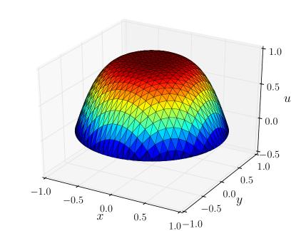
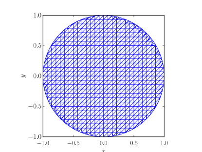
Figure 3: Reference solution $u$ and the cut finite element mesh in the circle geometry.

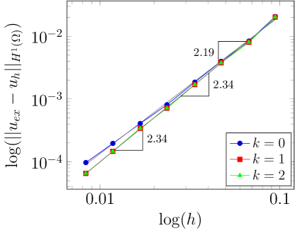
(a) a

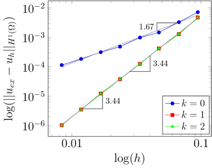
(b) a

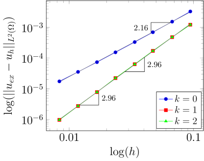
(c) a

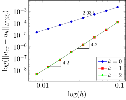
(d) a

Figure 4: Convergence rates for the first reference solution in the circle in the $H_{1}$ norm for $p=2$, LABEL:sub@subfig:_p3h1circle, $p=3$ for Taylor expansions of order $k=0,1,2$ and in the $L_{2}$ norm for LABEL:sub@subfig:_p2l2circle $p=2$,LABEL:sub@subfig:_p3l2circle $p=3$.

7.2 Reference Solution in Torus with Zero Dirichlet Boundary Conditions

Next, we consider a domain with convex and concave boundaries given by the zero level set of the function

$$\phi=\left(R-0.75\right)\left(R-0.25\right).$$ (33)

We set

$$f= 20\left(4-\frac{1}{R}\right)$$ (34)

and obtain the analytical solution

$$u=20\left(0.75-R\right)\left(R-0.25\right).$$ (35)

as shown in Figure 5. The convergence rates shown in Figure 6 are optimal for $p=2$, $p=3$ when a first order Taylor expansion is used in the boundary value correction terms.

(a)

(b)

Figure 5: Reference solution $u$ in a torus-like shaped geometry and the cut finite element mesh of the domain.

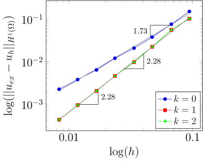
(a) a

(b) a

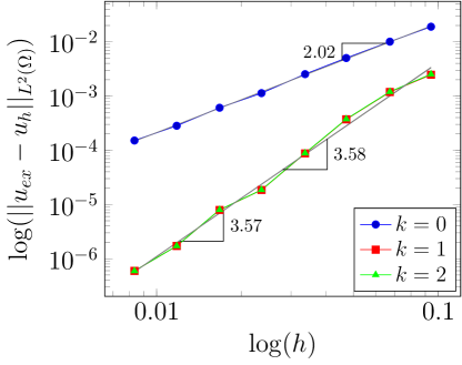
(c) a

(d) a

Figure 6: Convergence rates for the reference solution in the domain including convex and concave boundaries in the $H_{1}$ norm for LABEL:sub@subfig:_p2h1torus $p=2$, LABEL:sub@subfig:_p3h1torus, $p=3$ for Taylor expansions of order $k=0,1,2$ and in the $L_{2}$ norm for LABEL:sub@subfig:_p2l2torus $p=2$,LABEL:sub@subfig:_p3l2torus $p=3$.

7.3 Reference Solution in Flower Shape with Non-Zero Dirichlet Boundary Conditions

In our final example, we consider a flower like shaped domain  [17] defined by

$$\phi=(R^{2}-r_{\theta})(R^{2}-(1.0/6.0)^{2})$$ (36)

with $r_{\theta}=r_{0}+0.1\sin(\omega\theta)$, $r_{0}=1/2$, $\omega=8$ and $\theta=\arctan(x/y)$. We investigate the convergence rates of our numerical solution with respect to

$$u=\cos{\left(\pi\frac{x}{2}\right)}\cos{\left(\pi\frac{y}{2}\right)}$$ (37)

$$f=\frac{\pi^{2}}{2}\cos{\left(\pi\frac{x}{2}\right)}\cos{\left(\pi\frac{y}{2}\right)}$$ (38)

The reference solution and the cut mesh are shown in Figure 7. Figure 8 shows the convergence rate for $p=2$ and $p=3$.

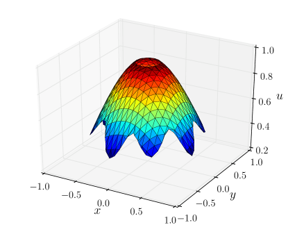
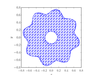
Figure 7: Reference solution $u$ in flower geometry and the cut finite element mesh of the domain.

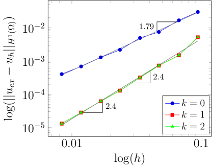
(a) a

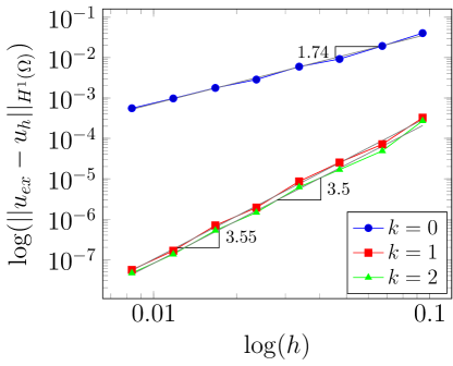
(b) a

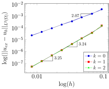
(c) a

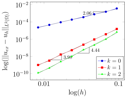
(d) a

Figure 8: Convergence rates for the reference solution in the flower shaped domain in the $H_{1}$ norm for LABEL:sub@subfig:_p2h1flower $p=2$, LABEL:sub@subfig:_p3h1flower, $p=3$ for Taylor expansions of order $k=0,1,2$ and in the $L_{2}$ norm for LABEL:sub@subfig:_p2l2flower $p=2$,LABEL:sub@subfig:_p3l2flower $p=3$.

7.4 3D Solution in an Ellipsoid

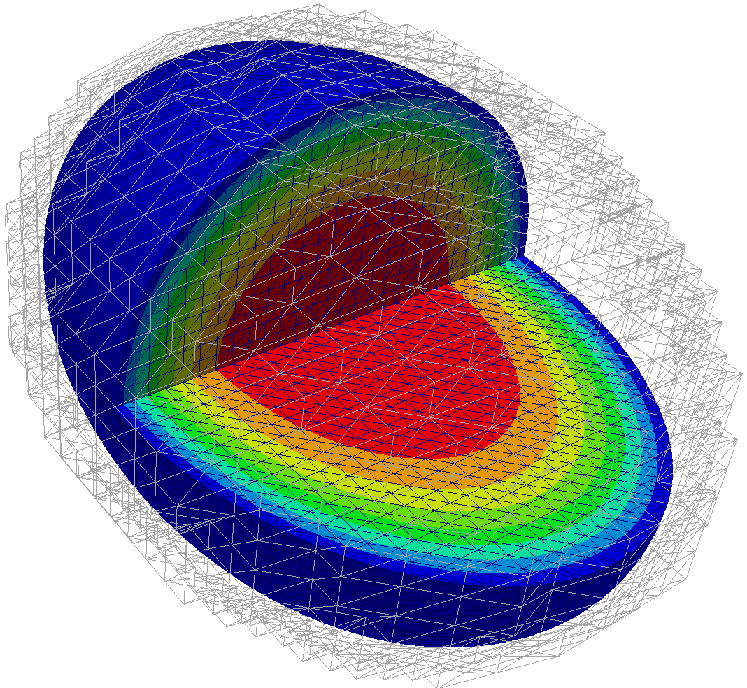
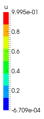
Figure 9: Reference solution $u$ in a 3D ellipsoid.

We compute the reference solution

$$u=\cos(\pi\frac{\hat{r}^{2}}{2})$$ (39)

with

$$\hat{r}=\sqrt{\frac{x^{2}}{(3.0/4.0)^{2}}+\frac{y^{2}}{(1.0/2.0)^{2}}+\frac{z^{2}}{(1.0/2.0)^{2}}}$$ (40)

in a 3D ellipsoid given by the function

$$\phi=\hat{r}-1.$$ (41)

Figure 9 shows the solution in the ellipsoid and Figure 10 shows the convergence for the solution for $p=2$ and $k=1$ demonstrating the optimal convergence rate of the numerical solution as predicted by the estimates of the previous section.

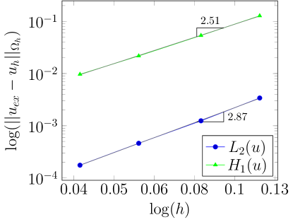
Figure 10: Error for $p=2$ in ellipsoid for $k=1$.

References

• [1] P. Angot, H. Lomenède and I. Ramière, A general fictitious domain method with non-conforming structured meshes, Finite volumes for complex applications IV, ISTE, London, 2005, pp. 261–272.
• [2] T. Boiveau and E. Burman, A penalty-free Nitsche method for the weak imposition of boundary conditions in compressible and incompressible elasticity, IMA Journal of Numerical Analysis (2015).
• [3] E. Burman, Ghost penalty, C. R. Math. Acad. Sci. Paris 348 (2010), 1217–1220.
• [4] E. Burman, A penalty free nonsymmetric Nitsche-type method for the weak imposition of boundary conditions, SIAM J. Numer. Anal. 50 (2012), 1959–1981.
• [5] E. Burman, S. Claus, P. Hansbo, M. G. Larson and A. Massing, CutFEM: Discretizing geometry and partial differential equations, International Journal for Numerical Methods in Engineering (2014), n/a–n/a.
• [6] E. Burman and M. A. Fernández, Explicit strategies for incompressible fluid-structure interaction problems: Nitsche type mortaring versus Robin-Robin coupling, Internat. J. Numer. Methods Engrg. 97 (2014), 739–758.
• [7] E. Burman and P. Hansbo, Fictitious domain finite element methods using cut elements: I. A stabilized Lagrange multiplier method, Comput. Methods Appl. Mech. Engrg. 199 (2010), 2680–2686.
• [8] E. Burman and P. Hansbo, Fictitious domain finite element methods using cut elements: II. A stabilized Nitsche method, Appl. Numer. Math. 62 (2012), 328–341.
• [9] E. Burman, P. Hansbo and M. G. Larson, A Cut Finite Element Method with Boundary Value Correction, (2015).
• [10] J. Freund and R. Stenberg, On weakly imposed boundary conditions for second order problems, in: Proceedings of the Ninth International Conference on Finite Elements in Fluids, pp. 327–336, Università di Padova, 1995.
• [11] V. Girault and R. Glowinski, Error analysis of a fictitious domain method applied to a Dirichlet problem, Japan Journal of Industrial and Applied Mathematics 12 (1995), 487–514 (English).
• [12] V. Girault, R. Glowinski and T. W. Pan, A fictitious-domain method with distributed multiplier for the Stokes problem, Applied nonlinear analysis, Kluwer/Plenum, New York, 1999, pp. 159–174.
• [13] A. Hansbo and P. Hansbo, An unfitted finite element method, based on Nitsche’s method, for elliptic interface problems, Comput. Methods Appl. Mech. Engrg. 191 (2002), 5537–5552.
• [14] J. Haslinger and Y. Renard, A New Fictitious Domain Approach Inspired by the Extended Finite Element Method, SIAM Journal on Numerical Analysis 47 (2009), 1474–1499.
• [15] T. J. R. Hughes, G. Engel, L. Mazzei and M. G. Larson, A comparison of discontinuous and continuous Galerkin methods based on error estimates, conservation, robustness and efficiency, Discontinuous Galerkin methods (Newport, RI, 1999), Lect. Notes Comput. Sci. Eng. 11, Springer, Berlin, 2000, pp. 135–146.
• [16] M. G. Larson and A. J. Niklasson, Analysis of a nonsymmetric discontinuous Galerkin method for elliptic problems: stability and energy error estimates, SIAM J. Numer. Anal. 42 (2004), 252–264 (electronic).
• [17] C. Lehrenfeld, High order unfitted finite element methods on level set domains using isoparametric mappings, Computer Methods in Applied Mechanics and Engineering 300 (2016), 716–733.
• [18] A. Massing, M. G. Larson, A. Logg and M. E. Rognes, A Stabilized Nitsche Fictitious Domain Method for the Stokes Problem, Journal of Scientific Computing 61 (2014), 604–628 (English).
• [19] J. Nitsche, Über ein Variationsprinzip zur Lösung von Dirichlet-Problemen bei Verwendung von Teilräumen, die keinen Randbedingungen unterworfen sind, Abhandlungen aus dem Mathematischen Seminar der Universität Hamburg 36 (1971), 9–15 (German).