Constraint-Preserving Scheme for Maxwell’s Equations

Abstract.

We derive the discretized Maxwell’s equations using the discrete variational derivative method (DVDM), calculate the evolution equation of the constraint, and confirm that the equation is satisfied at the discrete level. Numerical simulations showed that the results obtained by the DVDM are superior to those obtained by the Crank-Nicolson scheme. In addition, we study the two types of the discretized Maxwell’s equations by the DVDM and conclude that if the evolution equation of the constraint is not conserved at the discrete level, then the numerical results are also unstable.

1. Introduction

Constrained dynamical systems which are expressed by a set of evolution equations with constraints are important role in various branches of physics. For instance, the gauge theory is one of such systems, it is well known that the theory has been studied widely in the modern physics and mathematics. In addition, the canonical quantization of the constrained dynamical systems which is quantizing the Hamiltonian formalism in the classical theory was studied mainly by Dirac [1]. So the constrained dynamical systems are often formulated in the Hamiltonian formalism. If we analyze the constrained dynamical systems using simulations, it is not easy to conserve the constraints in the evolution. This is because the violations of the constraints caused by the numerical errors are grown in long-term free evolution. So we should make discretization of the equations using appropriate numerical schemes.

Recently, a number of investigations of schemes to derive suitable discretized equations have been reported. Some of these schemes are referred to as geometrical integration [2], in which the numerical errors in the initial state are preserved. The discrete variational derivative method (DVDM) is one such method. The DVDM was proposed then extended by Mori, Furihata, Matsuo, and Yaguchi [3, 4, 5, 6, 7, 8]. The method can apply the set of evolution equations which is derived by the variational principle in continuous level. If the set of the equations in continuous level have the dissipation and conservation properties, the set of discretized evolution equations using this method expects to preserve these properties. The DVDM is one of the methods of constructions of suitable numerical schemes, it would be possible to construct constraint preserving discrtized equations without the method. However, the idea is similar to the variational principle which is one of the most useful and powerful analytical tools in mathematics and physics. Therefore, this method seems to apply the various equations which have the Lagrangian and Hamiltonian density.

In this article, the purpose is finding the conditions to construct the appropriate discretization methods of the constrained systems. Especially, we target the types that the Hamiltonian density has the gauge freedoms, in other words the Hamiltonian density includes the constraints. So we select the Maxwell’s equations as the example. We seem the Maxwell’s equations are one of appropriate examples of the constrained dynamical systems. There are two reasons. First is that the equations are the linear with regard to the dynamical variables, we study easily relatively to the nonlinear cases. Second is that the structure is easily relatively to the one in modern physics such as the general relativity.

We organize our article as follows. In section 2, we review the Maxwell’s equations of the Hamiltonian formalism and derive the evolution equation of the constraint. In section 3, the brief reviews of the DVDM of the Hamiltonian formalism are shown. In section 4, we derive the three types of the discrete Maxwell’s equations. The one is using the ICNS, the others are using the DVDM. In section 5, we preform some simulations using the discretized equations made in Section 4, we summarize this article in Section 6. In this article, indices such as $(i,j,k,\cdots)$ run from 1 to 3. We use the Einstein convention of summation of repeated up-down indices. The indices are raised and lowered by the Kronecker delta.

2. Maxwell’s Equations

We begin by introducing the Maxwell’s equations and their Hamiltonian density. The equations are (e.g., see [10])

$$\epsilon_{0}\partial_{t}E_{i}-\frac{1}{\mu_{0}}\varepsilon_{i}{}^{mn}\partial_{m}B_{n} =-J_{i},$$ (1)

$$\partial_{t}B_{i}+\varepsilon_{i}{}^{mn}\partial_{m}E_{n} =0,$$ (2)

$$\partial_{i}E^{i} =\frac{1}{\epsilon_{0}}\rho,$$ (3)

$$\partial_{i}B^{i} =0,$$ (4)

where $\varepsilon_{ijk}$ is the Levi-Civita symbol and $E_{i}$ and $B_{i}$ are the electric field and magnetic flux density, respectively. $\epsilon_{0}$ and $\mu_{0}$ are the permittivity and the magnetic permeability in vacuum, respectively, which satisfy the relationship $\epsilon_{0}\mu_{0}=1/c^{2}$, where $c$ is the speed of light. $\rho$ and $J_{i}$ are the charge density and current density, respectively, which satisfy the equation of continuity

$$\partial_{t}\rho+\partial_{i}J^{i}=0.$$ (5)

The Lagrangian density of the Maxwell’s equations is defined as (see, e.g., [10, 11, 12])

$$\mathcal{L} \equiv\frac{\epsilon_{0}}{2}(E_{i}E^{i}-c^{2}B_{i}B^{i})-\rho\phi+J^{i}A_{i}$$

$$=\frac{\epsilon_{0}}{2}(\partial_{i}\phi+\partial_{t}A_{i})(\partial^{i}\phi+\partial_{t}A^{i})-\frac{1}{2\mu_{0}}(\partial^{a}A^{b}-\partial^{b}A^{a})(\partial_{a}A_{b})-\rho\phi+J^{i}A_{i},$$ (6)

where $\phi$ is the scalar potential and $A_{i}$ is the vector potential. $\phi$ and $A_{i}$ satisfy below the relationship

$$E_{i}=-\partial_{i}\phi-\partial_{t}A_{i},\quad B_{i}=\varepsilon_{i}{}^{mn}\partial_{m}A_{n}.$$ (7)

Then, we obtain the Hamiltonian density by the Legendre transformation (see, e.g., [12]) as,

$$\mathcal{H} \equiv\pi\partial_{t}\phi+\Pi^{i}\partial_{t}A_{i}-\mathcal{L}$$

$$=\phi(\rho+\partial_{i}\Pi^{i})+\frac{1}{2\epsilon_{0}}\Pi_{i}\Pi^{i}+\frac{1}{2\mu_{0}}(\partial^{a}A^{b}-\partial^{b}A^{a})(\partial_{a}A_{b})-J^{i}A_{i},$$ (8)

where $\pi\equiv(\delta\mathcal{L})/(\delta\partial_{t}\phi)$ and $\Pi^{i}\equiv(\delta\mathcal{L})/(\delta\partial_{t}A_{i})$ are the conjugate momenta of $\phi$ and $A_{i}$, respectively. They are written explicitly as

$$\pi =0,$$ (9)

$$\Pi^{i} =\epsilon_{0}(\partial^{i}\phi+\partial_{t}A^{i}).$$ (10)

Since $\pi=0$ identically, $\phi$ is a gauge variable. Therefore, the variation of $\mathcal{H}$ with $\phi$ is a constraint equation, i.e.,

$$0=-\frac{\delta\mathcal{H}}{\delta\phi}=-\rho-\partial_{i}\Pi^{i},$$ (11)

Consequently, the canonical formulation of the Maxwell’s equations is derived as

$$\mathcal{C} \equiv-\rho-\partial_{i}\Pi^{i},$$ (12)

$$\partial_{t}A_{i} \equiv\frac{\delta\mathcal{H}}{\delta\Pi^{i}}=-\partial_{i}\phi+\frac{1}{\epsilon_{0}}\Pi_{i},$$ (13)

$$\partial_{t}\Pi^{i} \equiv-\frac{\delta\mathcal{H}}{\delta A_{i}}=\frac{1}{\mu_{0}}\partial_{j}\partial^{j}A^{i}-\frac{1}{\mu_{0}}\partial_{j}\partial^{i}A^{j}+J^{i}.$$ (14)

The above set of equations is well-known the canonical formulation of the Maxwell’s equations [13](There are other formulations, e.g.,[14]). The details of the derivations are in A.

Equation (12) is consistent with Gauss’s law (3), and (14) is consistent with the Ampère law with Maxwell’s correction (1). Using (5), (13), and (14), the evolution equation of constraint $\mathcal{C}$ is calculated as

$$\partial_{t}\mathcal{C} =-\partial_{t}\rho-\partial_{t}\partial_{i}\Pi^{i}$$

$$=\partial_{i}J^{i}-\partial_{i}\left(\frac{1}{\mu_{0}}\partial_{j}\partial^{j}A^{i}-\frac{1}{\mu_{0}}\partial^{i}\partial_{j}A^{j}+J^{i}\right)$$

$$=0,$$ (15)

where the second equality is obtained using (5) and (14). From (15), (12) is guaranteed regardless of time. Hereafter, we call (15) the constraint propagation equation. Note that (15) is not derived from the functional derivative using the Hamiltonian density or the Lagrangian density.

3. Discrete Variational Derivative Method

Now we review the processes of deriving discretized equations using the DVDM, and further details of the DVDM are given in [6]. The discrete value of the variable $u$ is defined as $u{}^{(n)}_{(k)}$, where the upper index $(n)$ and lower index $(k)$ denote the time component and space component, respectively. The forward and backward difference operators are defined as $\widehat{\delta}^{+}_{i}u{}^{(n)}_{(k)}\equiv\bigl{(}u^{(n)}_{(k+1)}-u^{(n)}_{(k)}\bigr{)}/\Delta x^{i}$ and $\widehat{\delta}^{-}_{i}u{}^{(n)}_{(k)}\equiv\bigl{(}u^{(n)}_{(k)}-u^{(n)}_{(k-1)}\bigr{)}/\Delta x^{i}$, respectively, and the central difference operator is defined as $\widehat{\delta}^{\langle 1\rangle}_{i}\equiv(\widehat{\delta}^{+}_{i}+\widehat{\delta}^{-}_{i})/2$. The second-order central difference operator is defined as

$$\widehat{\delta}^{\langle 2\rangle}_{ij}u^{(n)}_{(k)}\equiv\left\{\begin{array}[]{ll}(u^{(n)}_{(k+1)}-2u^{(n)}_{(k)}+u^{(n)}_{(k-1)})/(\Delta x^{i})^{2},&(i=j)\\ \widehat{\delta}^{\langle 1\rangle}_{i}\widehat{\delta}^{\langle 1\rangle}_{j}u^{(n)}_{(k)}.&(i\neq j)\end{array}\right.$$

The symbol $\Delta x^{i}$ denotes $(\Delta x,\Delta y,\Delta z)$. Now, we show the standard process for discretizing equations. We adopt only the canonical formalism in this article, so that this process is only shown in the case that the generator function is the Hamiltonian density. The ordinary case is as follows: (A) We set a Hamiltonian density $\mathcal{H}(q_{i},p^{i})$ with variables $q_{i}$ and canonical conjugate momenta $p^{i}$. (B) The dynamical equations are given as

$$\partial_{t}q_{i} =\frac{\delta\mathcal{H}}{\delta p^{i}},\quad\partial_{t}p^{i}=-\frac{\delta\mathcal{H}}{\delta q_{i}},$$ (16)

and the discretized equations are constructed using a well-known method such as the Crank-Nicolson scheme. On the other hand, the process for the DVDM is as follows: (A^′) We set a discrete Hamiltonian density $\mathcal{H}^{(n)}_{(k)}\bigl{(}q_{i}{}^{(n)}_{(k)},p^{i}{}^{(n)}_{(k)}\bigr{)}$ with discrete variables $q_{i}{}^{(n)}_{(k)}$ and discrete canonical conjugate momenta $p^{i}{}^{(n)}_{(k)}$. (B^′) The discretized system obtained using the DVDM scheme is

$$\begin{array}[]{l}\displaystyle{\frac{q_{i}{}^{(n+1)}_{(k)}-q_{i}{}^{(n)}_{(k)}}{\Delta t}=\frac{\widehat{\delta}\mathcal{H}}{\widehat{\delta}(p^{i}{}^{(n+1)}_{(k)},p^{i}{}^{(n)}_{(k)})}},\\ \displaystyle{\frac{p^{i}{}^{(n+1)}_{(k)}-p^{i}{}^{(n)}_{(k)}}{\Delta t}=-\frac{\widehat{\delta}\mathcal{H}}{\widehat{\delta}(q_{i}{}^{(n+1)}_{(k)},q_{i}{}^{(n)}_{(k)})}},\end{array}$$ (19)

where $\widehat{\delta}\mathcal{H}/\bigl{(}\widehat{\delta}(p^{i}{}^{(n+1)}_{(k)},p^{i}{}^{(n)}_{(k)})\bigr{)}$ and $\widehat{\delta}\mathcal{H}/\bigl{(}\widehat{\delta}(q_{i}{}^{(n+1)}_{(k)},q_{i}{}^{(n)}_{(k)})\bigr{)}$ are calculated as

$$\mathcal{H}^{(n+1)}_{(k)}-\mathcal{H}^{(n)}_{(k)} =\frac{\widehat{\delta}\mathcal{H}}{\widehat{\delta}(p^{i}{}^{(n+1)}_{(k)},p^{i}{}^{(n)}_{(k)})}(p^{i}{}^{(n+1)}_{(k)}-p^{i}{}^{(n)}_{(k)})$$

$$\quad+\frac{\widehat{\delta}\mathcal{H}}{\widehat{\delta}(q_{i}{}^{(n+1)}_{(k)},q_{i}{}^{(n)}_{(k)})}(q_{i}{}^{(n+1)}_{(k)}-q_{i}{}^{(n)}_{(k)}).$$ (20)

The discrete value $\mathcal{H}^{(n)}_{(k)}$ is not defined uniquely; we can obtain different discretized equations depending on the definition. Thus, we should select an appropriate definition to obtain good simulation results.

4. Discrete Maxwell’s equations

In this section, we discretize the Maxwell’s equations in three ways. One way uses the iterative Crank-Nicolson scheme (ICNS), the others use the DVDM. We select the ICNS for comparing to the discretized equations using the DVDM. This is because that we can see clearly and easily the differences between the equations of ICNS and the ones of DVDM in the mathematical equations level. There are some degrees of freedom when deriving discretized equations by the DVDM, and we derive two sets of discretized equations. The first satisfies the constraint propagation equation at the discrete level, which we call System I. The other does not satisfy the equation, which we call System II.

4.1. Iterative Crank-Nicolson Scheme

The ICNS is one of the commonly used schemes to obtain discretized equations from (partial) differential equations. If we use this scheme, the evolution equations are discretized as the central difference in time and space. To obtain values at time step $n+1$ from those at time step $n$, it is used to do two iterations [15]. Then, the discretized Maxwell’s equations obtained using the ICNS are

$$\mathcal{C}^{(n)}_{(k)} =-\rho^{(n)}_{(k)}-\widehat{\delta}^{\langle 1\rangle}_{i}\Pi^{i}{}^{(n)}_{(k)},$$ (21)

$$\frac{A_{i}{}^{(n+1)}_{(k)}-A_{i}{}^{(n)}_{(k)}}{\Delta t} =-\frac{1}{2}\widehat{\delta}^{\langle 1\rangle}_{i}\left(\phi^{(n+1)}_{(k)}+\phi^{(n)}_{(k)}\right)+\frac{1}{2\epsilon_{0}}\left(\Pi_{i}{}^{(n+1)}_{(k)}+\Pi_{i}{}^{(n)}_{(k)}\right),$$ (22)

$$\frac{\Pi^{i}{}^{(n+1)}_{(k)}-\Pi^{i}{}^{(n)}_{(k)}}{\Delta t} =\frac{1}{2\mu_{0}}\widehat{\delta}^{\langle 2\rangle}_{j}{}^{j}\left(A^{i}{}^{(n+1)}_{(k)}+A^{i}{}^{(n)}_{(k)}\right)-\frac{1}{2\mu_{0}}\widehat{\delta}^{\langle 2\rangle}_{j}{}^{i}\left(A^{j}{}^{(n+1)}_{(k)}+A^{j}{}^{(n)}_{(k)}\right)$$

$$\quad+\frac{1}{2}\left(J^{i}{}^{(n+1)}_{(k)}+J^{i}{}^{(n)}_{(k)}\right),$$ (23)

and the equation of continuity is discretized using the ICNS as

$$\frac{\rho^{(n+1)}_{(k)}-\rho^{(n)}_{(k)}}{\Delta t} =-\frac{1}{2}\widehat{\delta}^{\langle 1\rangle}_{i}\left(J^{i}{}^{(n+1)}_{(k)}+J^{i}{}^{(n)}_{(k)}\right).$$ (24)

Using these equations, we calculate the discretized evolution equation of constraint $\mathcal{C}$ as

$$\frac{\mathcal{C}{}^{(n+1)}_{(k)}-\mathcal{C}{}^{(n)}_{(k)}}{\Delta t} =-\frac{\rho{}^{(n+1)}_{(k)}-\rho{}^{(n)}_{(k)}}{\Delta t}-\widehat{\delta}^{\langle 1\rangle}_{i}\frac{\Pi^{i}{}^{(n+1)}_{(k)}-\Pi^{i}{}^{(n)}_{(k)}}{\Delta t}$$

$$=-\frac{1}{2\mu_{0}}\widehat{\delta}^{\langle 1\rangle}_{i}\biggl{\{}\widehat{\delta}^{\langle 2\rangle}_{j}{}^{j}(A^{i}{}^{(n+1)}_{(k)}+A^{i}{}^{(n)}_{(k)})$$

$$\qquad-\widehat{\delta}^{\langle 2\rangle}_{j}{}^{i}(A^{j}{}^{(n+1)}_{(k)}+A^{j}{}^{(n)}_{(k)})\biggr{\}}.$$ (25)

The right-hand-side (r.h.s.) of this equation is not zero in general. For instance, if we set $\partial_{i}A_{j}=0\,\,(i\neq j)$ as the initial conditions, then the r.h.s. of (25) is zero. On the other hand, if we set $\partial_{i}A_{j}\neq 0\,\,(i\neq j)$ as the initial conditions, then the r.h.s of (25) is not zero. We will confirm the results that the simulations using ICNS may not work depending on the initial conditions by performing some simulations as reported in Sec 5.

4.2. System I

To derive discretized equations by the DVDM, we have to define the discretized Hamiltonian density appropriately. In this article, we define the discretized Hamiltonian density $\mathcal{H}^{(n)}_{(k)}$ as

$$\mathcal{H}^{(n)}_{(k)} \equiv-\Pi^{i}{}^{(n)}_{(k)}(\widehat{\delta}^{{\langle 1\rangle}}_{i}\phi^{(n)}_{(k)})+\frac{1}{2\epsilon_{0}}\Pi_{i}{}^{(n)}_{(k)}\Pi^{i}{}^{(n)}_{(k)}$$

$$\quad+\frac{1}{2\mu_{0}}(\widehat{\delta}^{{\langle 1\rangle}}{}^{i}A^{j}{}^{(n)}_{(k)}-\widehat{\delta}^{{\langle 1\rangle}}{}^{j}A^{i}{}^{(n)}_{(k)})({\delta}^{{\langle 1\rangle}}_{i}A_{j}{}^{(n)}_{(k)})+\rho^{(n)}_{(k)}\phi^{(n)}_{(k)}-J_{i}{}^{(n)}_{(k)}A^{i}{}^{(n)}_{(k)}.$$ (26)

Then the discretized Maxwell’s equations are derived using the DVDM as

$$\mathcal{C}^{(n)}_{(k)} =-\rho^{(n)}_{(k)}-\widehat{\delta}^{{\langle 1\rangle}}_{i}\Pi^{i}{}^{(n)}_{(k)},$$ (27)

$$\frac{A_{i}{}^{(n+1)}_{(k)}-A_{i}{}^{(n)}_{(k)}}{\Delta t} =-(\widehat{\delta}^{{\langle 1\rangle}}_{i}\phi^{(n+1)}_{(k)})+\frac{1}{2\epsilon_{0}}(\Pi_{i}{}^{(n+1)}_{(k)}+\Pi_{i}{}^{(n)}_{(k)}),$$ (28)

$$\frac{\Pi^{i}{}^{(n+1)}_{(k)}-\Pi^{i}{}^{(n)}_{(k)}}{\Delta t} =\frac{1}{2\mu_{0}}\widehat{\delta}^{{\langle 1\rangle}}{}_{j}\widehat{\delta}^{{\langle 1\rangle}}{}^{j}(A^{i}{}^{(n+1)}_{(k)}+A^{i}{}^{(n)}_{(k)})$$

$$\quad-\frac{1}{2\mu_{0}}\widehat{\delta}^{{\langle 1\rangle}}_{j}\widehat{\delta}^{{\langle 1\rangle}}{}^{i}(A^{j}{}^{(n+1)}_{(k)}+A^{j}{}^{(n)}_{(k)})+J^{i}{}^{(n)}_{(k)}.$$ (29)

Equation (5) is not derived from the functional derivative using the Hamiltonian density in the continuous case. Therefore, the discretized equation of continuity is also not derived from the DVDM; we define it as

$$\frac{\rho^{(n+1)}_{(k)}-\rho^{(n)}_{(k)}}{\Delta t}+\widehat{\delta}^{\langle 1\rangle}_{i}J^{i}{}^{(n)}_{(k)}=0.$$ (30)

Now, we show that $(\mathcal{C}^{(n+1)}_{(k)}-\mathcal{C}^{(n)}_{(k)})/\Delta t$ is always zero independent of the initial conditions. The discretized evolution of $\mathcal{C}^{(n)}_{(k)}$ is described by

$$\frac{\mathcal{C}^{(n+1)}_{(k)}-\mathcal{C}^{(n)}_{(k)}}{\Delta t} =-\frac{\rho^{(n+1)}_{(k)}-\rho^{(n)}_{(k)}}{\Delta t}-\widehat{\delta}^{\langle 1\rangle}_{i}\frac{\Pi^{i}{}^{(n+1)}_{(k)}-\Pi^{i}{}^{(n)}_{(k)}}{\Delta t}$$

$$=\widehat{\delta}^{\langle 1\rangle}_{i}J^{i}{}^{(n)}_{(k)}-\widehat{\delta}^{\langle 1\rangle}_{i}\biggl{\{}\frac{1}{2\mu_{0}}\widehat{\delta}^{\langle 1\rangle}_{j}\widehat{\delta}^{\langle 1\rangle}{}^{j}(A^{i}{}^{(n+1)}_{(k)}+A^{i}{}^{(n)}_{(k)})$$

$$\qquad-\frac{1}{2\mu_{0}}\widehat{\delta}^{\langle 1\rangle}_{j}\widehat{\delta}^{\langle 1\rangle}{}^{i}(A^{j}{}^{(n+1)}_{(k)}+A^{j}{}^{(n)}_{(k)})+J^{i}{}^{(n)}_{(k)}\biggr{\}}$$

$$=0,$$ (31)

where the second equality is obtained using (29) and (30). Equation (31) indicates that $\mathcal{C}^{(n)}_{(k)}$ does not change during the evolution. Therefore, we claim that the equations discretized using System I is better than that discretized using the ICNS.

4.3. System II

At the continuous level, the equation of continuity (5) is not derived from the Hamiltonian density (8). In the same way as at the discretized level, the discretized equation of continuity is also not derived. Thus, there are some degrees of freedom in deriving the discretized equations. Thus, for instance, if we replace $J^{i}{}^{(n)}_{(k)}$ by $J^{i}{}^{(n+1)}_{(k)}$ in (30):

$$\frac{\rho^{(n+1)}_{(k)}-\rho^{(n)}_{(k)}}{\Delta t}+\widehat{\delta}^{\langle 1\rangle}_{i}J^{i}{}^{(n+1)}_{(k)} =0.$$ (32)

Using (27)–(29) and (32), the discretized constraint propagation equation is

$$\frac{\mathcal{C}^{(n+1)}_{(k)}-\mathcal{C}^{(n)}_{(k)}}{\Delta t} =-\frac{\rho^{(n+1)}_{(k)}-\rho^{(n)}_{(k)}}{\Delta t}-\widehat{\delta}^{\langle 1\rangle}_{i}J^{i}{}^{(n)}_{(k)}$$

$$=-\widehat{\delta}^{\langle 1\rangle}_{i}(J^{i}{}^{(n)}_{(k)}-J^{i}{}^{(n+1)}_{(k)}).$$ (33)

This equation is NOT equal to zero in general. Therefore, we expect that the results of the simulations with System II will become unstable if the divergence of $J_{i}$ changes during the evolution.

To modify System II, the use of a new Hamiltonian density is possible. The result of the analysis of the discretized constraint propagation equation in the modified System II is only the same as that for System I, as shown in B.

5. Numerical Tests

In this section, using the ICNS and the two types of the DVDM: System I and System II, we perform some simulations in which we use two exact solutions of the Maxwell’s equations as the initial conditions. In these simulations, we take the permittivity and magnetic permeability as $\epsilon_{0}=\mu_{0}=1$ and the numerical parameters are set as follows:

• Simulation domain: $x,y,z\in[-0.5,0.5]$.

• Grid: $x_{i}=y_{i}=z_{i}=-0.5+(i-(1/2))dx$, $i=1,\dots,100$, where $dx=1/100$.

• Time step: $dt=0.1dx$.

• Iteration: Second-order iterative calculations in ICNS, System I, and System II.

• Gauge condition: Exact solution.

• Boundary condition: Periodic boundary condition.

The constraint preserving character of System I would be independent of the boundary condition, because that the discretized constraint propagation equation (31) is calculated without the boundary condition. In these simulations, since the characters of the scheme should be distinguished the ones caused by other conditions, we adopt only the boundary condition periodically.

The accuracies of the three schemes are all of second order in times and space, because that the difference operators $\delta^{{\langle 1\rangle}}_{i}$ and $\delta^{{\langle 2\rangle}}_{ij}$ are linear and second order in space. In addition, we confirm it in numerically with an initial data in C.

5.1. Case 1

First, we use the following exact solution of the Maxwell’s equations as the initial condition:

$$A_{i} =\frac{2\pi}{\omega^{2}}\begin{pmatrix}\cos(\omega t+2\pi x)\\ \sin(\omega t+2\pi y)\\ \omega^{2}\sin(2\pi z)\end{pmatrix},$$ (34)

$$\Pi^{i} =\frac{2\pi}{\omega}\begin{pmatrix}-\sin(\omega t+2\pi x)\\ \cos(\omega t+2\pi y)\\ -\omega t\sin(2\pi z)\end{pmatrix},$$ (35)

$$\phi =t\cos(2\pi z),$$ (36)

$$\rho =\frac{4\pi^{2}}{\omega}\{\cos(\omega t+2\pi x)+\sin(\omega t+2\pi y)+\omega t\cos(2\pi z)\},$$ (37)

$$J_{i} =-2\pi\begin{pmatrix}\cos(\omega t+2\pi x)\\ \sin(\omega t+2\pi y)\\ \sin(2\pi z)\end{pmatrix},$$ (38)

where $\omega=1$ and $t=1$. With this initial condition, the discretized constraint propagation equation of the ICNS (25) become zero because the vector potential $A_{i}$ satisfies the condition $\partial_{i}A_{j}=0\quad(i\neq j)$. Moreover, the divergence of $J_{i}$ is

$$\partial_{i}J^{i}=4\pi^{2}(\sin(\omega t+2\pi x)-\cos(\omega t+2\pi y)-\cos(2\pi z)),$$

and the discretized constraint propagation equation for System II (33) does not always become zero in the region $[-0.5,0.5]\times[-0.5,0.5]\times[-0.5,0.5]$.

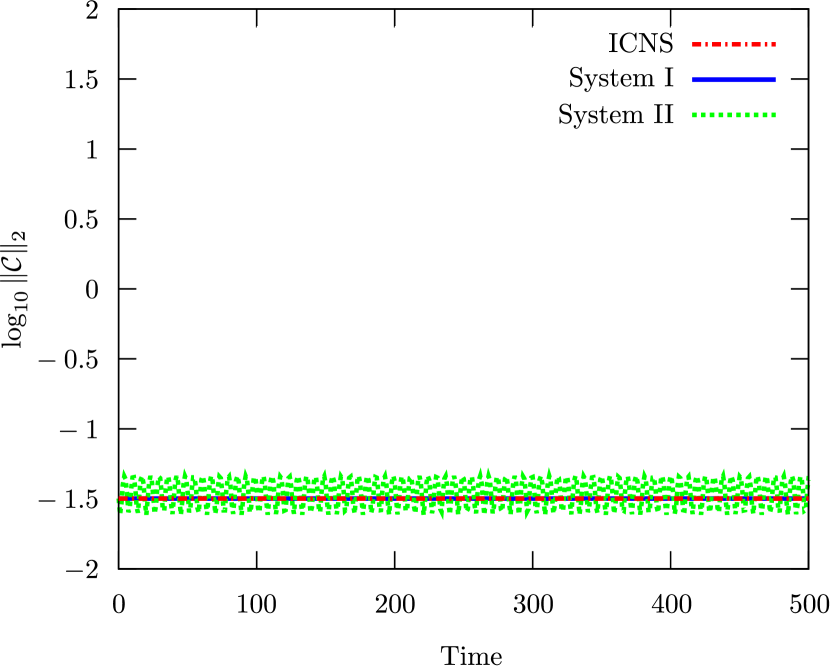
Figure 1. L2 norm of constraint $\mathcal{C}$ for the ICNS and the two types of DVDM (System I and System II). The vertical axis is the logarithm of $\mathcal{C}$ and the horizontal axis is time. The dot-dashed line represents the ICNS, the solid line represents the System I, and the dotted line represents the System II. The lines for the ICNS and System I overlap throughout the evolution.

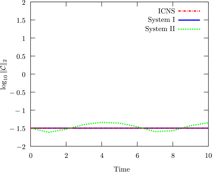
Figure 2. L2 norm of $\mathcal{C}$ drawn up to $t=10$. All numerical conditions are the same as those for Figure 1.

Figure 1 shows the L2 norm of constraint $\mathcal{C}$ for the ICNS (21)–(24), System I (27)–(30), and System II (27)–(29), (32). Figure 2 shows details of the interval up to $t=10$ in Figure 1. We see that the two lines for the ICNS and System I are unchanged during the evolution, whereas that for System II changes with time. These results are consistent with the previous analysis of the discretized constraint propagation equations. Figure 3 shows the solutions of $A_{3}$ of $t=5$, $-0.5\leq z\leq 0.5$ in three schemes. The bottom panel of the figures shows the details of the range $3.5\leq A_{3}\leq 6.5$ in the top panel.

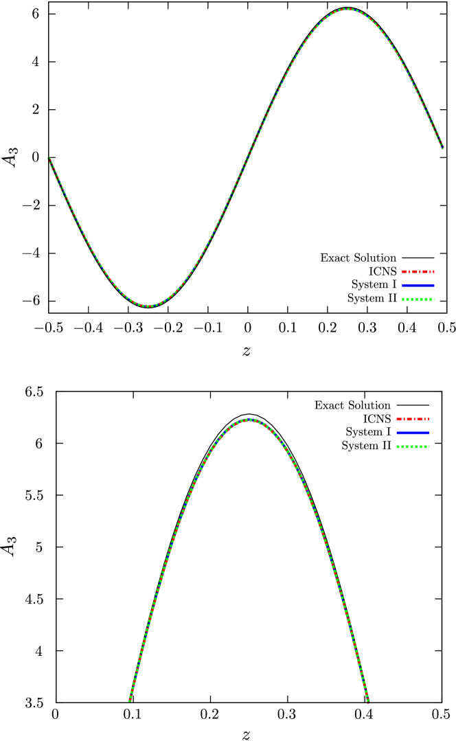
Figure 3. These lines express the solutions of $A_{3}$ at $t=5$. The vertical axis is $A_{3}$ and the horizontal axis is $z$. The top panel is drawn in $-0.5\leq z\leq 0.5$ and $-6.5\leq A_{3}\leq 6.5$, and the bottom panel is the one in $0\leq z\leq 0.5$ and $3.5\leq A_{3}\leq 6.5$. The thin line is drawn the exact solution, the dot-dashed line is using ICNS, the thick line is using System I, and the dotted line is using System II. The three lines except the thin line are overlapping.

In the figures, we see three lines using ICNS, System I, and System II are overlapping.

Figure 4. These lines express the solutions of $\rho$ at $t=5$, $x=-0.5$, $z=0$. The top panel is drawn in $-0.5\leq y\leq 0.5$ and $140\leq\rho\leq 230$. The thin line is drawn the exact solution, the dot-dashed line is using ICNS, the thick line is using System I, and the dotted line is using System II. All of the lines are almost overlapping. The bottom panel is drawn the relative errors of the three schemes against the exact solution. The dot-dashed line is drawn the relative errors of ICNS, the solid line is the ones of System I, and the dotted line is the ones of System II.

The top panel of Figure 4 shows the solutions of $\rho$ of $t=5$, $x=-0.5$, $z=0$, $-0.5\leq y\leq 0.5$ in three schemes. We see all the lines are almost overlapping. To see the differences of the schemes more details, we show the relative errors against the exact solution of the three schemes in the bottom panel of Figure 4. The differences between each value of the schemes hardly exist. For other conditions such as $t=10$ and other variables such as $\Pi^{i}$, the results are similar.

5.2. Case 2

Next, we use the following exact solution as the initial condition:

$$A_{i} =\frac{2\pi}{\omega^{2}}\begin{pmatrix}\cos(\omega t+2\pi x)\\ \sin(\omega t+2\pi y)\\ \omega^{2}\sin(2\pi(x+y+z))\end{pmatrix},$$ (39)

$$\Pi^{i} =\frac{2\pi}{\omega}\begin{pmatrix}-\sin(\omega t+2\pi x)\\ \cos(\omega t+2\pi y)\\ -\omega t\sin(2\pi z)\end{pmatrix},$$ (40)

$$\phi =t\cos(2\pi z),$$ (41)

$$\rho =\frac{4\pi^{2}}{\omega}\{\cos(\omega t+2\pi x)+\sin(\omega t+2\pi y)+\omega t\cos(2\pi z)\},$$ (42)

$$J_{i} =-2\pi\begin{pmatrix}\cos(\omega t+2\pi x)+4\pi^{2}\sin(2\pi(x+y+z))\\ \sin(\omega t+2\pi y)+4\pi^{2}\sin(2\pi(x+y+z))\\ \sin(2\pi z)-8\pi^{2}\sin(2\pi(x+y+z))\end{pmatrix},$$ (43)

where $\omega=1$ and $t=1$. The discretized constraint propagation equation with the ICNS (25) and that with System II (33) do not equal zero for this condition.

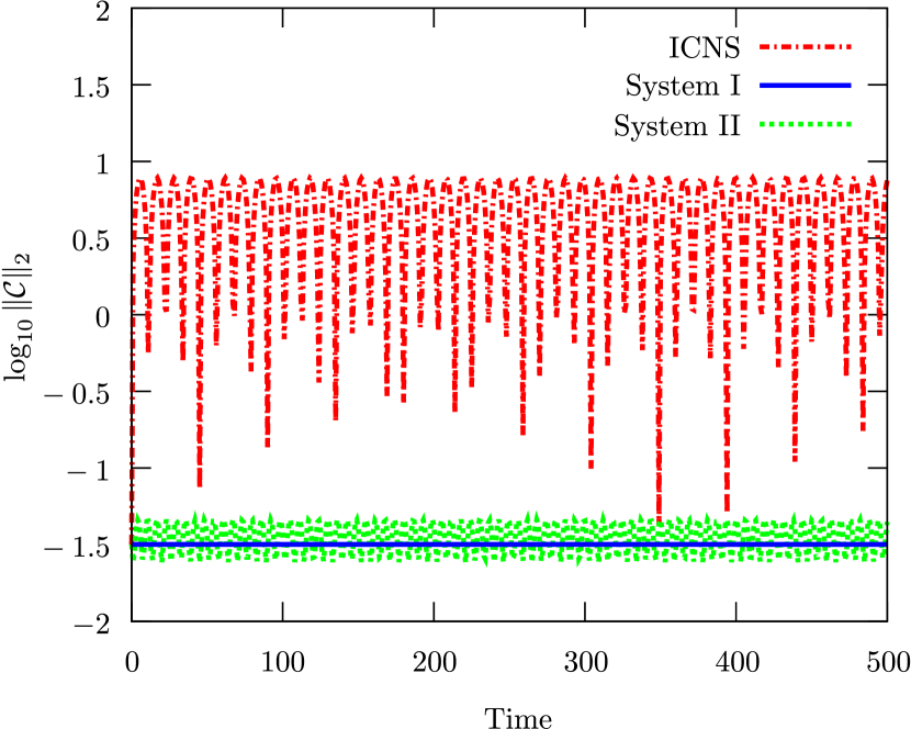
Figure 5. L2 norm of $\mathcal{C}$ for the same conditions as Figure 1 but with the initial condition given by (39)–(43). The lines representing the ICNS and System II oscillate and are unstable. On the other hand, the line for System I is unchanged from the initial state and is stable.

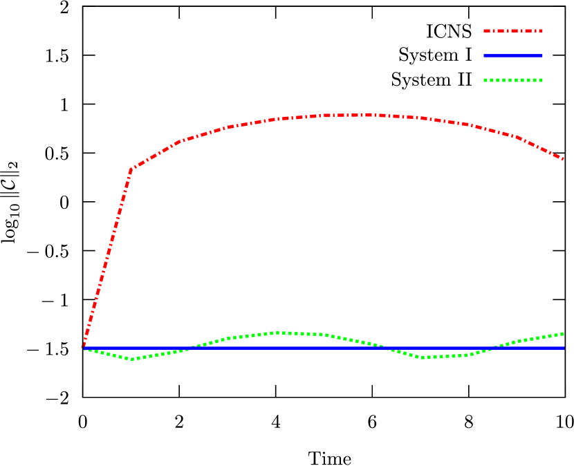
Figure 6. L2 norm of $\mathcal{C}$ is drawn up to $t=10$. All numerical conditions are the same as those for Figure 5.

Figure 5 is drawn under the same conditions as Figure 1 except for the initial condition. Figure 6 shows details of the interval up to $t=10$ in Figure 5. We see that the constraint violations of System I do not change during the evolution, meaning that the simulation is stable. On the other hand, those of the ICNS and System II are unstable. These results are consistent with the conclusions of the analysis at the discretized level in Sec. 4. Figure 7 shows the solutions of $A_{3}$ at $x=y=-0.5$ and Figure 8 shows the solutions of $\rho$ in the same conditions of Figure 3 and Figure 4, respectively, except the initial condition.

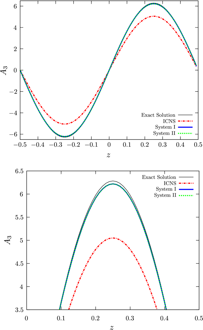
Figure 7. These lines express the solutions of $A_{3}$ at $x=y=-0.5$ in the same conditions of Figure 3 except the initial condition. The two lines using System I and System II are overlapping.

Comparing the differences between the lines of the three schemes and the exact solutions in Figure 7, we see the difference of ICNS is the largest. This is consistent with the Figure 5 and Figure 6. For the variables $A_{1},A_{2}$ and $\Pi^{i}$, the results are similar with the case of $A_{3}$.

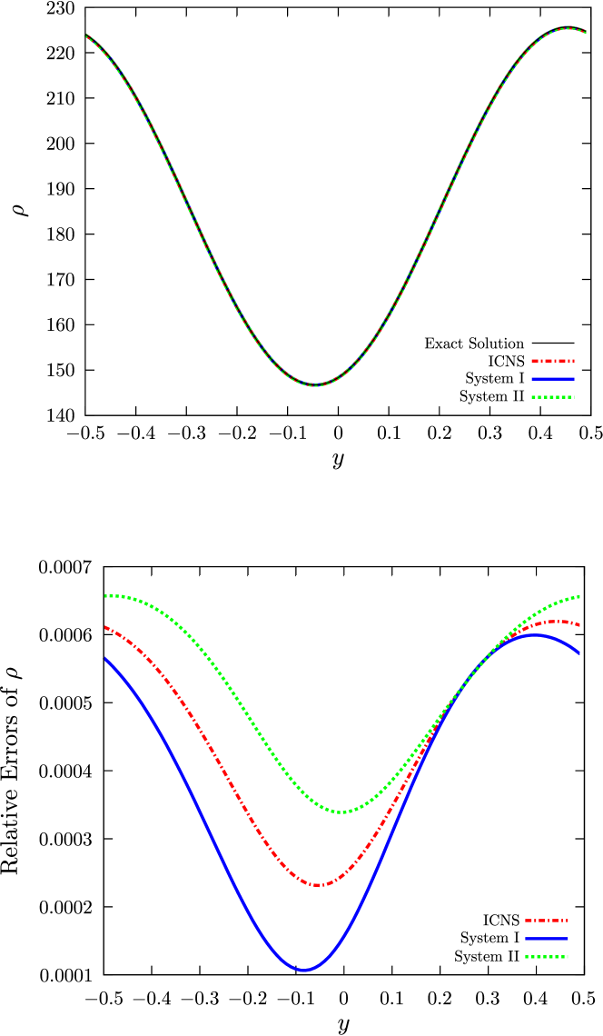
Figure 8. These lines express the solutions of $\rho$ in the same conditions of Figure 7 except the initial condition. The all lines of the top panel are almost overlapping.

In Figure 8, we see that the differences of the schemes are hardly.

6. Summary

To perform accurate simulations, we apply the discrete variational derivative method (DVDM) to the Maxwell’s equations to derive a new set of discretized Maxwell’s equations. In this process, we proposed a discretized Hamiltonian density and a discretized equation of continuity, showed that the constraint is unchanged at the discretized level, and confirmed this in some simulations. Comparing the numerical solutions and the exact solutions, we assert that the conservation of the constraint must be one of the important factors to get the precise numerical solutions. The definitions of the discretized Hamiltonian density and the discretized equation of continuity are not unique and are restricted to satisfy the constraint. A way of discretizing the equation of continuity was not obtained from the DVDM but from the analysis of the discretized constraint propagation equation. Therefore, we claim that we have found a way to appropriately define the discretized equation of continuity. We conclude that the analysis of the discretized constraint propagation equations is the key to perform accurate simulations in the constrained dynamical system.

In this article, we studied the Maxwell’s equations. There are some constrained dynamical systems except for the Maxwell’s equations. For instance, the Einstein’s field equations in general relativity is the one of such systems. Therefore we will construct appropriate discretized Einstein’s field equations by the DVDM in near the future.

Appendix A Derivation of the canonical formulation of Maxwell’s equations

The Hamiltonian density is as (8):

$$\mathcal{H}=\phi(\rho+\partial_{i}\Pi^{i})+\frac{1}{2\epsilon_{0}}\Pi_{i}\Pi^{i}+\frac{1}{2\mu_{0}}(\partial^{a}A^{b}-\partial^{b}A^{a})(\partial_{a}A_{b})-J^{i}A_{i},$$

then $A_{i}$, $\Pi^{i}$, and $\phi$ are independent variables. Since the $\delta\mathcal{L}/\delta(\partial_{t}\phi)$ is identically zero, $\phi$ is the gauge variable and the variation of $\phi$ is a constraint equation (12):

$$\mathcal{C}\equiv-\frac{\delta\mathcal{H}}{\delta\phi}=-\rho-\partial_{i}\Pi^{i}.$$

The variations of $\Pi^{i}$ and $A_{i}$ are the evolution equations of $A_{i}$ and $\Pi^{i}$, respectively, such as

$$\partial_{t}A_{i} \equiv\frac{\delta\mathcal{H}}{\delta\Pi^{i}}=\phi\partial_{i}+\frac{1}{\epsilon_{0}}\Pi_{i}=-\partial_{i}\phi+\frac{1}{\epsilon_{0}}\Pi_{i}+(\text{boundary terms}),$$

$$\partial_{t}\Pi^{i} \equiv-\frac{\delta\mathcal{H}}{\delta A_{i}}=-\frac{1}{2\mu_{0}}(\partial_{a}A_{b})(\delta^{bi}\partial^{a}-\delta^{ai}\partial^{b})-\frac{1}{2\mu_{0}}(\partial^{a}A^{b}+\partial^{b}A^{a})\delta^{i}{}_{b}\partial_{a}+J^{i}$$

$$=\frac{1}{\mu_{0}}\partial_{j}\partial^{j}A^{i}-\frac{1}{\mu_{0}}\partial_{j}\partial^{i}A^{j}+J^{i}+(\text{boundary terms}),$$

the boundary terms in the above equations can be vanished in a suitable boundary condition, then we can get the equation (13) and (14), respectively:

$$\partial_{t}A_{i} =-\partial_{i}\phi+\frac{1}{\epsilon_{0}}\Pi_{i},$$

$$\partial_{t}\Pi^{i} =\frac{1}{\mu_{0}}\partial_{j}\partial^{j}A^{i}-\frac{1}{\mu_{0}}\partial_{j}\partial^{i}A^{j}+J^{i}.$$

Appendix B Modified equations of System II

To make the discretized constraint propagation equations of System II equal to zero, we replace $J_{i}{}^{(n)}_{(k)}$ with $J_{i}{}^{(n+1)}_{(k)}$ in the Hamiltonian density (26); thus, we redefine the discretized Hamiltonian density as

$$\bar{\mathcal{H}}^{(n)}_{(k)} \equiv-\Pi^{i}{}^{(n)}_{(k)}(\widehat{\delta}^{{\langle 1\rangle}}_{i}\phi^{(n)}_{(k)})+\frac{1}{2\epsilon_{0}}\Pi_{i}{}^{(n)}_{(k)}\Pi^{i}{}^{(n)}_{(k)}$$

$$\quad+\frac{1}{\mu_{0}}(\widehat{\delta}^{{\langle 1\rangle}}{}^{i}A^{j}{}^{(n)}_{(k)}-\widehat{\delta}^{{\langle 1\rangle}}{}^{j}A^{i}{}^{(n)}_{(k)})(\widehat{\delta}^{{\langle 1\rangle}}{}_{i}A_{j}{}^{(n)}_{(k)})+\rho^{(n)}_{(k)}\phi^{(n)}_{(k)}-J_{i}{}^{(n+1)}_{(k)}A^{i}{}^{(n)}_{(k)},$$ (44)

then the discretized Maxwell’s equations are derived by the DVDM as (27) (28) and

$$\frac{\Pi_{i}{}^{(n+1)}_{(k)}-\Pi_{i}{}^{(n)}_{(k)}}{\Delta t} =J_{i}{}^{(n+1)}_{(k)}+\frac{1}{2\mu_{0}}\widehat{\delta}^{{\langle 1\rangle}}{}_{a}\widehat{\delta}^{{\langle 1\rangle}}{}^{a}(A_{i}{}^{(n+1)}_{(k)}+A_{i}{}^{(n)}_{(k)})$$

$$\quad-\frac{1}{2\mu_{0}}\widehat{\delta}^{{\langle 1\rangle}}_{a}\widehat{\delta}^{{\langle 1\rangle}}_{i}(A^{a}{}^{(n+1)}_{(k)}+A^{a}{}^{(n)}_{(k)}).$$ (45)

We refer to (27), (28), (45), and (32) as System III. The discretized constraint propagation equation of System III is equal to zero. The results of numerical simulations using System III were expected to be the same as the those System I. We performed some simulations using System III for Case 1 and Case 2 in Sec. 5 as the initial conditions and confirmed that the constraint violations of System III are consistent with those of System I.

However, the Hamiltonian density (44) is unnatural because the $(n+1)$th time component is included. Therefore, we should define the discretized Hamiltonian density as (26) and the discretized equation of continuity as (30).

Appendix C Convergence Test of System I and System II in Case II

We show that the both of the convergences in the System I and System II are second order of $\Delta x$ and $\Delta t$.

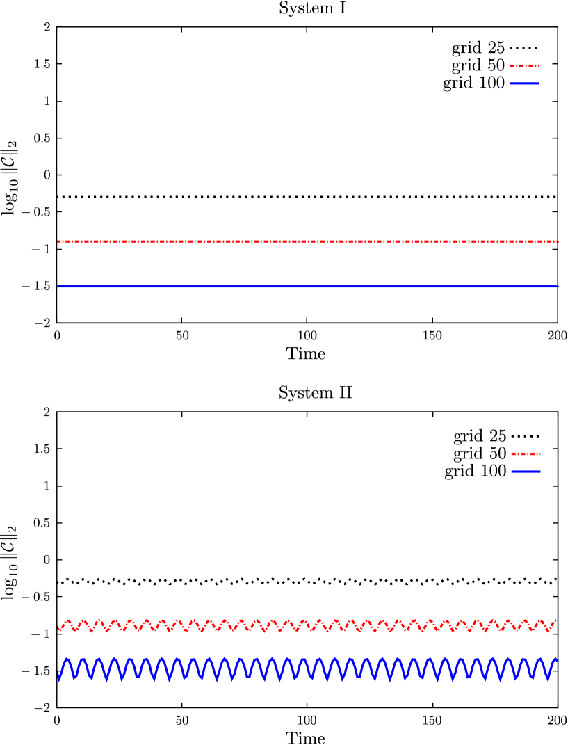
Figure 9. Upper panel is drawn using System I, lower panel is using System II. The vertical axis is the logarithm of $\mathcal{C}$ and the horizontal axis is time. The dotted line is drawn in the grid as $\Delta x=\Delta y=\Delta z=1/25$, the dot-dashed line drawn in $\Delta x=\Delta y=\Delta z=1/50$, and the solid line drawn in $\Delta x=\Delta y=\Delta z=1/100$. $\log_{10}\|\mathcal{C}\|_{2}$ of the dotted line is around $-0.3$, the one of the dot-dashed line is around $-0.9$, and the one of the dotted line is around $-1.5$.

The top panel and the bottom panel in Figure 9 are drawn using System I and System II, respectively, in the initial condition as Case II. We can see the differences between $\log_{10}\|\mathcal{C}\|_{2}$ of the grids are $0.6\approx\log_{10}4$, these results indicate that both of the convergence properties of the systems are second order in time and space.

References

- [1] P. A. M. Dirac, Lectures on Quantum Mechanics (Belfer Graduate School of Sciencs, Yeshiva University, New York, 1964).
- [2] H. Hairer and C. Lubich, Geometric Numerical Integration (Springer, 2010).
- [3] D. Furihata and M. Mori, ZAMM Z. angew. Math. Mech. 76, 405 (1996).
- [4] D. Furihata, J. Comput. Phys. 156, 181 (1999).
- [5] T. Matsuo and D. Furihata, J. Comput. Phys. 171, 425 (2001).
- [6] D. Furihata and T. Matsuo, Discrete Variational Derivative Method (CRC Press, 2010).
- [7] Y. Aimoto, T. Matsuo, and Y. Miyatake, Discrete Contin. Dyn. Syst. 8, 817 (2015).
- [8] A. Ishikawa and T. Yaguchi, JSIAM Lett. 7, 17 (2015).
- [9] D. Alic, C. Bona-Casas, C. Bona, L. Rezzolla, and C. Palenzuela, Phys. Rev. D 85, 064040 (2012).
- [10] J. A. Jackson, Classical Electrodynamics (Wiley, 1975).
- [11] F. E. Low, Classical Field Theory (Wiley-Interscience, 1997).
- [12] R. M. Wald, General Relativity (University of Chicago Press, 1984).
- [13] W. K. H. Panofsky and M. Phillips, Classical Electricity and Megnetism: Second Edition, (Addison-Wesley, 1962).
- [14] N. Anderson and A. M. Arthurs, Int. J. Electronis, 1983, 54, 861, (1978).
- [15] S. A. Teukolsky, Phys. Rev. D 61, 087501 (2000).