Weiss oscillations in graphene with a modulated height profile

Abstract

We study the electronic transport properties of a monolayer graphene with a one-dimensional modulated height profile caused, for instance, by substrate ondulations. We show that the combined effect of the resulting strain fields induce modulated scalar and vector potentials that give rise to Weiss oscillations in the magnetoconductivity. We also find that similar effects can be obtained by applying a parallel magnetic field to the graphene-substrate interface. The parameters of an experimental set-up for a physical realization of these findings in graphene systems are discussed.

I Introduction

The magnetoresistivity of a two-dimensional electron gas (2DEG) subjected to a periodic potential varying in one direction shows very strong oscillations periodic in inverse magnetic field Weiss et al. (1989). This remarkable effect, called Weiss oscillations, is observed in the magnetoresistivity parallel to the grating direction of the periodic potential and is negligible on the transversal and longitudinal directions. The effect was quantitatively in terms of the semiclassical electronic velocity obtained from the quantum mechanical analysis of the changes in the local band structure due to the modulated potential Winkler et al. (1989); Gerhardts et al. (1989); Vasilopoulos and Peeters (1989); Peeters and Vasilopoulos (1992). The Weiss oscillations can also be understood using a classical approach that associates their periodicity with the commensurability of the cyclotron motion and the grating, which modifies the root-mean-square of the drift velocity of the guiding center Beenakker (1989). This gives origin to oscillations of the magnetoresistivity with period $2R_{c}/\lambda$, where $R_{c}$ is the cyclotron radius and $\lambda$ is the period of the grating. This nice and intuitive picture is corroborated by the solution of the Boltzmann equation, assuming both an isotropic Beenakker (1989) and anisotropic Mirlin and Wölfle (1998) disorder scattering processes.

Several theoretical works studied Weiss oscillations in graphene systems. Using the quantum mechanical approach Winkler et al. (1989); Gerhardts et al. (1989); Vasilopoulos and Peeters (1989); Peeters and Vasilopoulos (1992), oscillations in the magnetoconductivity were calculated for the cases of monolayer graphene sheet modulated magnetic Tahir and Sabeeh (2008) and electric field Matulis and Peeters (2007); Tahir et al. (2007); Tahir and Sabeeh (2007). The theory of Weiss oscillations was also extended to bilayer graphene Zarenia et al. (2012). These studies put in evidence the similarities and the differences between Weiss oscillations in graphene and 2DEG systems. One of the conclusions is that one expects the effect to be more robust against temperature in graphene, due to its unique spectral properties. Unfortunately, there is no experimental report of Weiss oscillations in graphene so far.

The main goal of this paper is to propose a set-up that allows to experimentally observe the effect. Assuming a given modulated profile height varying along a single-direction we explore two mechanisms that give rise to a periodic potential, namely, strain and/or an in-plane external magnetic applied on the graphene sheet.

Strain modifies the interatomic distances and, hence, the electronic structure of the material. Combining an effective microscopic model for the low-energy properties of electrons in graphene with the theory of elasticity, it has been shown Suzuura and Ando (2002); Mañes (2007); Guinea et al. (2008); Castro Neto et al. (2009); Vozmediano et al. (2010); Masir et al. (2013) that the effects due to strain fields can be accounted for by a pseudo electric and pseudo magnetic fields, that are incorporated to the effective graphene Hamiltonian as a diagonal scalar and vector potentials, respectively. Recent papers have shown that these pseudo fields give measurable contributions for transport propertiesCouto et al. (2014); Burgos et al. (2015).

A magnetic field applied parallel to the modulated grephene sheet can also generate an effective periodic vector potential as long as $\lambda$ is much larger that the height profile amplitude, as discussed in Refs. Lundeberg and Folk, 2010; Burgos et al., 2015. Experimentally, modulated profile heights have been reported in suspended membranes Bao et al. (2009) and nanoripples Lee et al. (2013); Bai et al. (2014). Another possibility is to lithographically produce trenches, defining a profile height on a given substrate. After deposition, the graphene sheet acquires a similar shape.

This paper is organized as follows. Section II begins with a brief review of the effective theory of the low energy dynamics of electrons in graphene under a uniform perpendicular magnetic field. We discuss the modulated pseudomagnetic and pseudo electric fields due to strain in Section II.1. The expression for the modulated parallel magnetic field is obtained in Section II.2. In Section III we present analytical closed expressions for the Weiss oscillations due to modulated pseudo electric and pseudo magnetic fields In Section IV we present our main results, discuss the validity range of the theory, establishing bounds to guide an optimal choice of the experimental set-up parameters to study the effect. Finally we present our conclusions in Section V.

II Theoretical background

Our model Hamiltonian reads

$$H=H_{0}+H^{\prime},$$ (1)

where $H_{0}$ accounts for the dynamics of low-energy electrons in graphene monolayers under a uniform external magnetic field and $H^{\prime}$ is the effective Hamiltonian due to the modulated deformation of the graphene sheet.

In the presence of an external applied magnetic field, the effective Hamiltonian for low energy electrons in graphene reads Castro Neto et al. (2009); Goerbig (2011)

$$H_{0}=v_{F}\bm{\sigma}\cdot\left({\bm{p}}+e{\bm{A}}_{\rm ext}\right),$$ (2)

where $v_{F}\approx 10^{6}$m/s is the Fermi velocity and $\bm{\sigma}=(\sigma_{x},\sigma_{y})$ are Pauli matrices in the lattice subspace Castro Neto et al. (2009).

For a uniform magnetic field perpendicular to the graphene plane, $\bm{B}_{\rm ext}=B_{\perp}\hat{{\bf z}}$, the vector potential can be written in the Landau gauge

$$\bm{A}_{\rm ext}=B_{\perp}[(1-\alpha)y\hat{\bm{x}}+\alpha x\hat{\bm{y}}].$$ (3)

We postpone the discussion of the most convenient choice of $\alpha$ to the next section.

In what follows we obtain the effective perturbation Hamiltonian $H^{\prime}$ that describes the effects of strain due to a periodic out-of-plane deformation of the graphene sheet given by

$$h(x)=h_{0}\cos(2\pi x/\lambda),$$ (4)

where $\lambda$ is the modulation period and $h_{0}$ is the profile height amplitude.

II.1 Strain induced magnetic and electric fields

Strain modifies the graphene inter-atomic distances and changes its electronic properties. It has been shown Suzuura and Ando (2002); Mañes (2007); Midtvedt et al. (2016) that strain effects in the electronic dynamics can be accounted for by introducing a vector gauge potential and a scalar potential in the effective Hamiltonian given by Eq. (2).

By taking the long wavelength limit of the graphene tight-binding Hamiltonian the strain contribution to the system Hamiltonian, up to linear order in the deformations, can be cast as Suzuura and Ando (2002); Mañes (2007); de Juan et al. (2013)

$$H^{\prime}=t\sum_{n=1}^{3}i\frac{\bm{\sigma}\cdot\bm{\delta}_{n}}{a}\sigma_{z}\left(\frac{\beta_{\rm G}}{a^{2}}\bm{\delta}_{n}^{T}\cdot\bm{u}\cdot\bm{\delta}_{n}\right),$$ (5)

where ${\bm{\delta}}_{n}$ are the nearest neighbor vectors (see Fig. 1), $a\approx 1.42$ Å is the carbon-carbon distance, $t\approx 2.7$ eV is the nearest neighbor $\pi$-orbitals hopping matrix element, and $\beta_{\rm G}=-\partial\log t/\partial\log a\approx 2-3.37$ Guinea et al. (2008); Pereira et al. (2009) is the Grüneisen parameter, a dimensionless material dependent parameter that characterizes the coupling between the Dirac electrons and the lattice deformations, and $\bm{u}$ is the strain tensor.

We express the components of the strain tensor in the “macroscopic” $xy$ coordinate system. The lattice sites are more conveniently assigned by “intrinsic” $x^{\prime}y^{\prime}$ coordinates oriented along the high symmetry crystallographic directions of the graphene lattice, as shown in Fig. 1a.

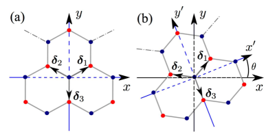
Figure 1: (Color online) Honeycomb lattice orientation: (a) zigzag crystallographic orientation along the $x$-axis and (b) arbitrary orientation.

In the intrinsic coordinate system the nearest neighbor vectors read Castro Neto et al. (2009)

$$\bm{\delta}_{1}=\frac{a}{2}\left(\!\begin{array}[]{c}\sqrt{3}\\ 1\end{array}\!\right),\;\bm{\delta}_{2}=\frac{a}{2}\left(\!\begin{array}[]{c}-\sqrt{3}\\ 1\end{array}\!\right),\;\bm{\delta}_{3}=a\left(\!\begin{array}[]{c}0\\ -1\end{array}\!\right).$$ (6)

For the case where $xy$ and $x^{\prime}y^{\prime}$ coincide, by inserting the relations for ${\bm{\delta}}$ into Eq. (5), the strain contribution to the system Hamiltonian becomes

$$H^{\prime}=ev_{F}{\bm{\sigma}}\cdot{\bm{A}},$$ (7)

with

$${\bf A}=\frac{\hbar\beta_{\rm G}\kappa}{2ae}\left(\begin{array}[]{c}u_{xx}-u_{yy}\\ -2u_{xy}\end{array}\right),$$ (8)

where $\kappa\approx 2/3$ stands for the correction of the graphene effective vector potential due to the violation of the Cauchy-Born rule in lattices with a basis Suzuura and Ando (2002); Midtvedt et al. (2016).

Let us now consider the more realistic case where the graphene zigzag crystal orientation forms an angle $\theta$ with the “macroscopic” $x$-axis, see Fig. 1b. Accordingly, the nearest neighbor vectors ${\bm{\delta}}_{n}$ are rotated by $\theta$, namely

$${\bm{\delta}}_{n}(\theta)={\bf R}(\theta)\cdot{\bm{\delta}}_{n},$$ (9)

where ${\bf R}(\theta)$ is the rotation matrix in two-dimensions. Inserting the rotated nearest neighbor vectors ${\bm{\delta}}_{n}(\theta)$ in Eq. (5) we obtain

$${\bf A}(\theta)=\frac{\hbar\beta_{\rm G}\kappa}{2ae}\left(\begin{array}[]{c}(u_{xx}-u_{yy})\cos 3\theta+2u_{xy}\sin 3\theta\\ (u_{xx}-u_{yy})\sin 3\theta-2u_{xy}\cos 3\theta\end{array}\right)$$ (10)

or, in a more compact form,

$${\bf A}(\theta)={\bf R}(3\theta)\cdot{\bf A}.$$ (11)

We note that, with few exceptions Mucha-Kruczynski and Fal’ko (2012); Oliva-Leyva and Naumis (2015); Verbiest et al. (2015), the literature addresses only the perfect aligned case of $\theta=0$.

In addition to the pseudo vector potential, strain also induces a scalar potential Suzuura and Ando (2002); von Oppen et al. (2009); Midtvedt et al. (2016) given by

$$V(\bm{r})=g[u_{xx}(\bm{r})+u_{yy}(\bm{r})]I,$$ (12)

where $I$ is the identity matrix in sublattice space and $g\approx 4$ eV Guinea et al. (2010).

The strain tensor components $u_{ij}(\bm{r})$ read Suzuura and Ando (2002); Mañes (2007); Guinea et al. (2008)

$$u_{xx}({\bm{r}}) =\frac{\partial u_{x}(\bm{r})}{\partial x}+\frac{1}{2}\!\left[\frac{\partial h({\bm{r}})}{\partial x}\right]^{2},$$

$$u_{yy}({\bm{r}}) =\frac{\partial u_{y}(\bm{r})}{\partial y}+\frac{1}{2}\!\left[\frac{\partial h({\bm{r}})}{\partial y}\right]^{2},$$

$$u_{xy}({\bm{r}}) =\frac{1}{2}\left[\frac{\partial u_{x}(\bm{r})}{\partial y}+\frac{\partial u_{y}(\bm{r})}{\partial x}\right]+\frac{1}{2}\frac{\partial h({\bm{r}})}{\partial x}\frac{\partial h({\bm{r}})}{\partial y}.$$ (13)

The in-plane displacement vector field ${\bm{u}}(\bm{r})$ can be obtained, for instance, by minimizing the elastic energy Wehling et al. (2008); Guinea et al. (2008) for a given $h(\bm{r})$, following the prescription proposed in Ref. Guinea et al., 2008.

For one-dimensional periodic modulations, such as $h(x)$ defined by Eq. (4), the minimization of the elastic energy leads to a relaxed configuration where the strain tensor components become negligibly small Wehling et al. (2008). Such analysis does not account for the fact that, in general, the graphene sheet is pinned to the substrate at random positions Ishigami et al. (2007) that introduce non trivial constraints on the in-plane displacements. In this paper we consider quenched ripples, setting $u_{x}(\bm{r})=u_{y}(\bm{r})=0$. We stress that this assumption gives an upper bound of the strain field and to the corresponding vector gauge potential.

The strain tensor corresponding to the out-of-plane deformation profile $h(x)$ described by Eq. (4) reads

$$u_{xx}(x) = 2\pi^{2}\left(\frac{h_{0}}{\lambda}\right)^{2}\sin^{2}(2\pi x/\lambda),$$

$$u_{yy}(x) = u_{xy}(x)=0.$$ (14)

Hence, the pseudo vector potential reads

$${\bf A}(\theta)=A_{0}\sin^{2}(2\pi x/\lambda)\left(\begin{array}[]{c}\cos 3\theta\\ \sin 3\theta\end{array}\right)$$ (15)

where

$$A_{0}=\frac{\hbar\beta_{\rm G}\pi^{2}\kappa}{ae}\left(\frac{h_{0}}{\lambda}\right)^{2}.$$ (16)

The pseudo scalar potential is given by

$$V(x)=V_{0}\sin^{2}(2\pi x/\lambda),$$ (17)

with

$$V_{0}=2g\pi^{2}\left(\frac{h_{0}}{\lambda}\right)^{2}.$$ (18)

We finish this section recalling that theoretical studies Gibertini et al. (2012); Mucha-Kruczynski and Fal’ko (2012) show that the scalar potential is dramatically screened by the carriers in the graphene flake. Screening modifies the coupling $g$ as $g\rightarrow g/\epsilon(\bm{q},\omega\rightarrow 0)$, where $1/\epsilon(\bm{q},\omega)=1+v(\bm{q})\Pi^{R}(\bm{q},\omega)$ with $\epsilon(\bm{q},\omega)$ the dynamical dielectric function, $v(\bm{q})=2\pi e^{2}/\epsilon_{0}|\bm{q}|$ the Coulomb interaction with $\epsilon_{0}$ being the substrate material dependent dielectric constant, and $\Pi^{R}(\bm{q},\omega)$ is the retarded density-density correlation function. Within the random phase approximation (RPA) the dielectric function can be expressed as $\epsilon(\bm{q},\omega)=1-u(\bm{q})\chi^{0}(\bm{q},\omega),$ where $\chi^{0}(\bm{q},\omega)$ is the pair bubble diagram. The static dielectric function reads Hwang and Das Sarma (2007)

$$\epsilon(\bm{q},0)=\left\{\begin{array}[]{ll}1+v(\bm{q})\rho(E_{F}),&\ q\leq 2k_{F},\\ 1+v(\bm{q})\rho(E_{F})\Bigg{[}1-\frac{1}{2}\sqrt{1-\left(\frac{2k_{F}}{q}\right)^{2}}\\ \;\;\;\;\;\;\;\;\;\;\;-\frac{q}{4k_{F}}\arcsin\left(\frac{2k_{F}}{q}\right)+\frac{\pi q}{8k_{F}}\Bigg{]},&\,\,q>2k_{F}.\end{array}\right.$$ (19)

with $\rho(E_{F})$ the density of states at the Fermi energy. We have checked that $\epsilon(\bm{q},0)\gtrsim 40$ for graphene deposited on silicon dioxide, suggesting that screening can strongly quench the pseudoelectric field. Based on this reasoning, it has been conjectured Gibertini et al. (2012) that the random ripples, ubiquitous in deposited exfoliated graphene, are the cause of the charge puddles observed in these systems. Scanning tunneling microscopy (STM) experiments on graphene on SiO₂ Deshpande et al. (2009); Zhang et al. (2009) do not find evidences of spacial correlations between ripples and charge puddles and, thus, fail to support this picture.

In what follows we assume that screening is absent, corresponding to an upper bound of the scalar potential. We address again the screening issue in Sec. IV, where we discuss an experimental set-up to measure Weiss oscillations.

II.2 External in-plane magnetic field

A modulated magnetic field can also be realized by applying an external magnetic field parallel to a grated patterned graphene sheet. The external magnetic field has a component perpendicular to the graphene surface profile given by Burgos et al. (2015)

$$B^{\prime}({\bm{r}})=-{\bm{B}}_{\parallel}\cdot\hat{\bm{n}}({\bm{r}}).$$ (20)

The normal vector to the surface $z=h({\bm{r}})$ is

$$\hat{\bm{n}}({\bm{r}})=\frac{1}{\sqrt{1+(\partial h/\partial x)^{2}+(\partial h/\partial y)^{2}}}\left(\begin{array}[]{c}\partial h({\bm{r}})/\partial x\\ \partial h({\bm{r}})/\partial y\\ -1\end{array}\right).$$ (24)

Since $h_{0}\ll\lambda$, we write

$$\hat{\bm{n}}({\bm{r}})\approx(\partial h({\bm{r}})/\partial x,\partial h({\bm{r}})/\partial y,-1)^{T}.$$ (25)

Hence, the effective local perpendicular magnetic field reads

$$B_{\rm ext}({\bm{r}})=-{\bm{B}}_{\parallel}\cdot{\bm{\nabla}}h({\bm{r}}),$$ (26)

that for $\bm{B}_{\parallel}=B_{\parallel}\hat{\bm{x}}$ is expressed in a convenient gauge, by the vector potential

$$A_{x}({\bm{r}})=0\quad\mbox{and}\quad A_{y}({\bm{r}})=-A_{\|}\cos(2\pi x/\lambda)\,.$$ (27)

with $A_{\|}=B_{\|}h_{0}$. The perturbation term is given by

$$V_{\rm ext}(\bm{r})=v_{F}e\sigma_{y}A_{y}({\bm{r}})=-v_{F}eA_{\|}\cos(2\pi x/\lambda)\sigma_{y}.$$ (28)

III Weiss oscillations in graphene

In this section we briefly review the calculations of the Weiss oscillations for modulated magnetic Tahir and Sabeeh (2008) and electric Matulis and Peeters (2007) fields, adapting the results to the vector and scalar fields obtained in the previous section.

We study the corrections to the conductivity caused by the modulated strain within the regime where the latter corresponds to a small perturbation of the electronic spectrum. In this case, one can obtain an analytical expression for the Weiss conductivity oscillations following the approach put forward in Refs. Winkler et al., 1989; Gerhardts et al., 1989; Vasilopoulos and Peeters, 1989.

The scalar potential of Eq. (17) breaks the translational invariance along the $x$-axis. Hence, it is convenient to solve the unperturbed Hamiltonian $H_{0}$ in the Landau gauge with $\alpha=1$. Hence, the Schrödinger equation $H_{0}\Psi(\bm{r})=E\Psi(\bm{r})$ has eigenvalues McClure (1956); Castro Neto et al. (2009); Goerbig (2011)

$$E_{n}={\rm sgn}(n)\,\hbar\omega_{0}\sqrt{2|n|},$$ (29)

with $\omega_{0}=v_{F}/l_{B}$ and

$${\rm sgn}(n)=\left\{\begin{array}[]{ll}1&\,\,n>0,\\ 0&\,\,n=0,\\ -1&\,\,n<0.\end{array}\right.$$ (30)

The corresponding eigenfunctions are Zheng and Ando (2002)

$$\Psi_{n,k_{y}}(\bm{r})=\frac{C_{n}}{\sqrt{L_{y}l_{B}}}e^{ik_{y}y}\begin{pmatrix}-i{\rm sgn}(n)\Phi_{|n|-1}(\frac{x-x_{0}}{l_{B}})\\ \Phi_{|n|}(\frac{x-x_{0}}{l_{B}})\end{pmatrix},$$ (31)

where $l_{B}=\sqrt{\hbar/eB}\approx(26\,{\rm nm})/\sqrt{B({\rm T})}$ is the magnetic length, $x_{0}=l_{B}^{2}k_{y}$ gives the center of the wave function,

$$C_{n}=\left\{\begin{array}[]{ll}1&n=0,\\ 1/\sqrt{2}&n\neq 0,\end{array}\right.$$ (32)

and

$$\Phi_{n}(x)=\frac{e^{-x^{2}/2}}{\sqrt{2^{n}n!\sqrt{\pi}}}H_{n}(x),$$ (33)

where $H_{n}(x)$ are Hermite polynomials.

Starting from the Kubo formula for the conductivity, it has been shown Peeters and Vasilopoulos (1992) that the main contribution to the Weiss oscillations comes from the diagonal diffusive conductivity, that in the quasielastic scattering regime can be written as Charbonneau et al. (1982)

$$\Delta\sigma_{yy}=g_{v}g_{s}\frac{e^{2}}{L_{x}L_{y}}\sum_{\zeta}\left.\left(-\frac{\partial f}{\partial\varepsilon}\right)\right|_{\varepsilon=E_{\zeta}}\tau(E_{\zeta})v_{\zeta,y}v_{\zeta,y},$$ (34)

where $g_{v}$ and $g_{s}$ stand for valley and spin degeneracy (for graphene $g_{v}g_{s}=4$), $\zeta=(n,k_{y})$ are the quantum numbers of the single-particle electronic states, $L_{x}$ and $L_{y}$ are the dimensions of the graphene layer, $f(E_{\zeta})$ is the Fermi-Dirac distribution function, $\tau(E_{\zeta})$ is the electron relaxation time, and $v^{\zeta}_{y}$ is the electron velocity given by the semiclassical relation

$$v_{\zeta,y}=\frac{1}{\hbar}\frac{\partial}{\partial k_{y}}E_{n,k_{y}},$$ (35)

with $E_{n,k_{y}}$ calculated in first order perturbation theory as

$$E_{n,k_{y}}=E_{n}+\langle n,k_{y}|H^{\prime}|n,k_{y}\rangle.$$ (36)

Note that this correction lifts the degeneracy of Landau levels. The dc diffusive conductivity is then obtained by explicitly summing over the quantum numbers, namely

$$\sum_{\zeta}\big{[}\cdots\big{]}=\frac{L_{y}}{2\pi}\int^{L_{x}/l_{B}^{2}}_{0}dk_{y}\sum_{n=0}^{\infty}\big{[}\cdots\big{]}.$$ (37)

III.1 Modulated scalar potential

Let us now present the theory for Weiss oscillations for graphene monolayers in a modulated electric field Matulis and Peeters (2007). We highlight the main results that are relevant to our analysis, deferring the details of the derivation to the original literature Matulis and Peeters (2007).

For the scalar potential, the expectation value of the velocity operator $v_{\zeta,y}^{\rm s}=\hbar^{-1}\partial\langle n,k_{y}|V|n,k_{y}\rangle/\partial k_{y}$ reads

$$v_{\zeta,y}^{\rm s} =\frac{2\pi V_{0}l_{B}^{2}}{\hbar\lambda}e^{-u/2}$$

$$\times[{\rm sgn}^{2}(n)L_{|n|-1}(u)+L_{|n|}(u)]\sin\left(4\pi\frac{x_{0}}{\lambda}\right),$$ (38)

where $u=8\pi^{2}(l_{B}/\lambda)^{2}$ and $L_{n}(u)$ is a Laguerre polynomial.

Inserting the above expression in Eq. (34) and using (37), $\Delta\sigma_{yy}$ reads

$$\Delta\sigma^{\rm s}_{yy}\approx\frac{e^{2}}{h}\frac{V^{2}_{0}\beta\tau}{\hbar}F^{\rm s}(u,\beta,E_{F})$$ (39)

with

$$F^{\rm s}= \frac{ue^{-u}}{\beta}\sum^{\infty}_{n=-\infty}\left.\left(-\frac{\partial f}{\partial\varepsilon}\right)\right|_{\varepsilon=E_{n}}\!\!$$

$$\times[(1-\delta_{0,n})L_{|n|-1}(u)+L_{|n|}(u)]^{2}$$ (40)

where $\beta=1/k_{B}T$. We assume that $\Delta E_{n,k_{y}}=|E_{n,ky}-E_{n}|$ is smaller than the Landau level spacing and take $\tau=\tau(E_{F})$.

Equation (34) indicates that $\Delta\sigma_{yy}$ is dominated by the Landau levels with energies close to the Fermi energy. In the limit where many Landau levels are either filled (for $E_{F}>0$) or empty (for $E_{F}<0$), it is possible Matulis and Peeters (2007) to obtain an analytical expression for $\Delta\sigma_{yy}^{\rm s}$. First, one uses the $n\gg 1$ asymptotic expression for the Laguerre polynomials Szegö (1955)

$$e^{-u/2}L_{n}(u)\longrightarrow\frac{1}{\pi^{1/2}(nu)^{1/4}}\cos(2\sqrt{nu}-\pi/4),$$ (41)

that is very accurate as long as $u\lesssim n$. For $n\lesssim u\lesssim 4n$ the Laguerre polynomial is still an oscillatory function, but shows significant deviations from the expression given by Eq. (41) Temme (1990). For $u\gtrsim 4n$ the $L_{n}(u)$ is monotonic. For the Landau levels $n$ close to the Fermi energy, $u\gtrsim 4n$ is translated to $k_{F}\lambda\lesssim 2\pi$, where the electrons become insensitive to the modulated potential, a regime that is hardly relevant for the realistic physical parameters, as discussed in the next section.

Next, one takes the continuum limit

$$\sum_{n=-\infty}^{\infty}\big{[}\cdots\big{]}\approx\left(\frac{l_{B}}{v_{F}\hbar}\right)^{2}\int_{-\infty}^{\infty}dEE\big{[}\cdots\big{]}.$$ (42)

After some algebra we write

$$F^{\rm s}=\frac{1}{\pi^{2}}\frac{T}{T_{\rm W}}\cos^{2}\!\left(\frac{2\pi}{k_{F}\lambda}\right)\left[1+S\!\left(\frac{T}{T_{\rm W}}\right)\sin\!\left(8\pi\frac{k_{F}l^{2}_{B}}{\lambda}\right)\right],$$ (43)

where

$$S(x)=\frac{x}{\sinh(x)}\quad\text{and}\quad k_{\rm B}T_{\rm W}=\frac{\hbar\omega_{0}}{8\pi^{2}}\frac{\lambda}{l_{B}}.$$ (44)

III.2 Modulated vector potential

Let us now turn our attention to the conductivity corrections due to magnetic modulations.

In the case of the pseudo vector potential caused by strain, the expectation value of the velocity operator is

$$v^{\rm v}_{\zeta,y} =A_{0}\frac{l_{B}v_{F}e}{\hbar}{\sqrt{2}}\cos\!\left(\frac{4\pi}{\lambda}x_{0}\right)$$ (45)

$$\times e^{-u/2}{\rm sgn}(n)\sqrt{|n|+1}\left[L_{|n|+1}(u)-L_{|n|}(u)\right]\sin(3\theta),$$

where $u=8\pi^{2}(l_{B}/\lambda)^{2}$ and $L_{n}(u)$ is a Laguerre polynomial. Inserting the results of Eqs. (45) and (49) in Eq. (34) and using (37), the $\Delta\sigma^{\rm v}_{yy}$ reads

$$\Delta\sigma^{\rm v}_{yy}\approx\frac{e^{2}}{h}\frac{(v_{F}eA_{0})^{2}\tau\beta}{\hbar}\sin^{2}(3\theta)\,F^{\rm v}(u,\beta,E_{F})$$ (46)

with

$$F^{\rm v}= \frac{4e^{-u}}{\beta}\sum^{\infty}_{n=-\infty}\!\!\left.\left(-\frac{\partial f}{\partial\varepsilon}\right)\right|_{\varepsilon=E_{n}}\!\!(1-\delta_{0,n})(|n|+1)$$

$$\times\left[L_{|n|}(u)-L_{|n|+1}(u)\right]^{2}.$$ (47)

Following the steps described in the scalar potential case, we obtain

$$F^{\rm v}= \frac{1}{4\pi^{4}}(\lambda k_{F})^{2}\frac{T}{T_{\rm W}}\sin^{2}\!\left(\frac{2\pi}{k_{F}\lambda}\right)$$

$$\times\left[1-S\!\left(\frac{T}{T_{\rm W}}\right)\sin\left(8\pi\frac{k_{F}l^{2}_{B}}{\lambda}\right)\right],$$ (48)

where $S(x)$ and $T_{\rm W}$ are defined in Eq. (44).

For the case of an external in-plane magnetic field, the expectation of the velocity operator is

$$v^{\|}_{\zeta,y}= A_{\|}\frac{l_{B}v_{F}e}{\hbar}\sqrt{2}\cos\left(\frac{2\pi}{\lambda}x_{0}\right)$$ (49)

$$\times e^{-u/2}{\rm sgn}(n)\sqrt{|n|+1}\left[L_{|n|+1}(u)-L_{|n|}(u)\right],$$

with $u=2\pi^{2}(l_{B}/\lambda)^{2}$. Note that the functional dependence of $v^{\|}_{\zeta,y}$ is very similar to the one of Eq. (45), except for the periodicity which differs by a factor 2. This observation allows us to readily write the conductivity correction for the case of an external modulated magnetic field as

$$\Delta\sigma^{\rm\|}_{yy}\approx\frac{e^{2}}{h}\frac{(v_{F}eA_{\|})^{2}\tau\beta}{\hbar}F^{\|}(u,\beta,E_{F})$$ (50)

where $F^{\|}(u,\beta,E_{F})$ is obtained by taking $\lambda\rightarrow 2\lambda$ in the expression for $F^{\rm v}(u,\beta,E_{F})$.

IV Results and discussion

In this section we discuss the validity range of our results and propose bounds for the parameter range of a set-up to realize the Weiss oscillations in graphene systems. We analyze separately the cases of Weiss oscillations caused by strain and those due to a parallel magnetic field. We discuss their combined effect in a realistic experimental setup.

We note that the obtained expressions for the Weiss oscillations are consistent with the semiclassical guiding-center-drift resonant picture due to Beenakker Beenakker (1989), that predicts

$$\frac{\Delta\rho_{xx}}{\rho_{xx}}\propto\cos^{2}\left(2\pi\frac{R_{c}}{\lambda^{*}}-\frac{\pi}{4}\right),$$ (51)

where $R_{c}$ is the cyclotron radius and $\lambda^{*}$ the periodicity of the modulated potential. In the semiclassical regime of $n\gg 1$, one can safely neglect zitterbewegung effects Cserti and Dávid (2006); Schliemann (2008) and write $R_{c}=\hbar k_{F}/eB=\sqrt{2n}l_{B}$, in line with recent cyclotron orbits imaging observations Bhandari et al. (2016). By recalling that $\lambda^{*}=\lambda/2$, one immediately identifies that the periodicity of the Weiss oscillations of Eq. (51) coincides with the expressions presented in the previous section. This observation, so far overlooked in the graphene literature, suggests that the classical commensurability orbit resonance picture still holds in Dirac-like materials, as graphene.

Let us now address the main assumption of the analysis presented in Sec. III and discuss their implications.

(i) Semiclassical regime: We address disordered graphene samples characterized by an electronic elastic mean free path $\ell$. The electronic transport is considered as diffusive, with sample sizes $L\gg\ell$, and semiclassical, with $k_{F}\ell\gg 1$. Under these assumptions, the conductivity can be predicted with good accuracy by Eq. (34). For good quality graphene samples, where $\ell\geq 100$ nm, $k_{F}\ell\gg 1$ demands typical carrier concentrations $|n_{e}|\geq 10^{11}$cm^-2, which is easy to attain in experiments.

(ii) Perturbation theory: The evaluation of $\Delta\sigma_{yy}$ relies on using first order perturbation theory to calculate the semiclassical electron velocities $v_{\zeta,y}$, Eq. (35). Hence, it requires the Landau level spacing to be much larger than the energy correction due to the modulated perturbation potential. The Landau levels that contribute to the conductivity are those close to the Fermi energy, corresponding to

$$n_{F}\approx\frac{1}{2}\left(\frac{E_{F}}{\hbar\omega_{0}}\right)^{2}=\frac{1}{2}\left(k_{F}l_{B}\right)^{2}.$$ (52)

The applicability of the perturbation theory demands that the LL spacing $E_{n+1}-E_{n}$ is large as compared with the correction $\Delta E_{n}$ given by Eq. (36).

Let us consider the contributions due to strain and parallel magnetic field separately. For the scalar potential, $E_{n+1}-E_{n}>\Delta E_{n}$ constraints the Landau levels index $n$ to

$$n<\frac{2}{\pi^{4}}\left(\frac{\lambda}{l_{B}}\right)^{2}\left(\frac{\hbar v_{F}}{g\lambda}\right)^{4}\left(\frac{\lambda}{h_{0}}\right)^{8},$$ (53)

where we assume $n\gg 1$. Using Eq. (52), the above relation can be conveniently cast as

$$k_{F}l_{B}<\frac{2}{\pi^{2}}\left(\frac{\lambda}{l_{B}}\right)\left(\frac{\hbar v_{F}}{g\lambda}\right)^{2}\left(\frac{\lambda}{h_{0}}\right)^{4}.$$ (54)

The profile height parameters that govern the potential modulation enter the expression mainly as a $\lambda/h_{0}$ ratio, but the remaining quantities appear in a convoluted manner. We note that $k_{F}=\sqrt{\pi|n_{e}|}$ gives some freedom to easily fulfill the inequality by tuning the doping.

For the case of modulated magnetic fields, $E_{n+1}-E_{n}>\Delta E_{n}$ restricts $n$ to

$$n<\left[\left(\frac{\hbar\pi}{2Ae\lambda}\right)^{4}\left(\frac{8\pi^{4}l^{2}_{B}}{\lambda^{2}}\right)\right]^{1/3},$$ (55)

where $A$ = $A_{0}$ corresponds to the intrinsic pseudo magnetic case, while $A=A_{\|}$ stands for the external parallel magnetic field one. Using Eq. (52) we write

$$\frac{\pi}{4}\left(\frac{\beta_{\rm G}\kappa l_{B}}{2a}\right)^{4/3}|n_{e}|<\left[\left(\frac{\lambda^{2}}{h^{8}_{0}}\right)\right]^{1/3}.$$ (56)

for the case of strain generated gauge field and

$$\frac{\pi}{4}\left(\frac{eB_{\|}l_{B}}{2\hbar\pi^{2}}\right)^{4/3}|n_{e}|<\left[\left(\frac{1}{h^{4}_{0}\lambda^{6}}\right)\right]^{1/3},$$ (57)

for the external parallel magnetic field.

(iii) Asymptotic limit: In Sec. III, Eq. (41) is used to obtain a closed analytical expression for the conductivity oscillations. This asymptotic expression for the Laguerre polynomials requires that $n\gg 1$ and $\lambda/\lambda_{F}\geq 4$. In Fig. 2 we compare the “analytic” $\Delta\sigma_{yy}$, calculated using Eq. (III.2), with the “numeric” $\Delta\sigma_{yy}$ obtained from the numerical calculation of Eq. (III.2) for a representative set of parameters. We observe that by decreasing the magnitude of the perpendicular magnetic field, corresponding to increasing $n$, the agreement between the analytical and the numerical results progressively improves, as expected. For small magnetic fields the agreement depends on $\lambda/\lambda_{F}$, as explained Sec. III.1. The inset shows $\Delta\sigma^{||}_{yy}$ versus $1/B$ for a case where $\lambda/\lambda_{F}\approx 1$. The Weiss oscillations persist, but their period show a small deviation from our analytical results and the slope displays a more pronounced difference.

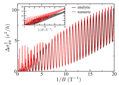
Figure 2: (Color online) External magnetic field contribution to the transversal conductivity $\Delta\sigma^{||}_{yy}$ as a function of $1/B$ for an electronic density of $n_{e}=5\times 10^{11}$ cm^-2, $\lambda=100$ nm, $h_{0}=1$ nm, $B_{\|}=8$ T, $T=4$ K, and $\tau=10^{-13}$s. Inset: Same parameters, except $\lambda=50$ nm.

To study the combined effect of the three modulated potentials considered in this paper, we use Eq. (34) with the total velocity

$$v^{\rm T}_{\zeta,y}=v^{\rm s}_{\zeta,y}+v^{\rm v}_{\zeta,y}+v^{\|}_{\zeta,y}.$$ (58)

Following the same steps as before, we write the conductivity as a sum of three independent contributions

$$\Delta\sigma_{yy}=\Delta\sigma^{\rm s}_{yy}+\Delta\sigma^{\rm v}_{yy}+\Delta\sigma^{\|}_{yy},$$ (59)

since upon integration over $k_{y}$ the cross terms average to zero. We show the three contributions separately in Fig. 3. For the sake of definition, $\Delta\sigma^{v}_{yy}$ represents an average over all possible lattice orientations. For a given experimental realization it is possible to measure the angle $\theta$.

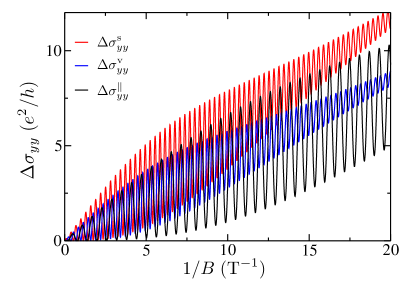
Figure 3: (Color online) Magnetoconductivity $\Delta\sigma^{||}_{yy}$ as a function of $1/B$ for the three modulated perturbation potentials discussed in the text. Here we use $B_{\|}=8$T, $\lambda=100$nm, $h_{0}=1$nm, $T=4$K, and $\tau\approx 10^{-13}$s.

Figure 3 indicates that, for the chosen set of parameters, all considered mechanisms contribute with similar weights to the Weiss oscillations. We caution that our strain calculations represent an upper limit, since we neglect atomic in-plane relaxations and screening. Hence, we expect the in-plane magnetic field to be the most efficient way to study the effect. On the other hand, in view of the large quantitative uncertainty on the degrees of screening and in-plane relaxation in actual systems, the investigation of Weiss oscillations in the absence of $B_{||}$ has the potential to provide interesting insight on this issue.

In a realistic situation, a good description of the height profile certainly requires considering more than a single-harmonic. In such case the different contributions to the conductivity oscillations no longer decouple. Notwithstanding, it is still easy to single-out the external parallel magnetic field oscillations by varying $B_{||}$. For moderate values of $B_{||}$ we expect this contribution to dominate over pseudo-fields generated by strain.

Let us now discuss the temperature dependence. Figure 4 shows the effect of the damping term $S(T/T_{W})$ on the oscillation amplitude of $\Delta\sigma_{yy}$ for few representative temperatures. Note that $T_{W}\propto B$. Hence, for a fixed $T$, by decreasing $B$, one decreases $T_{W}$ and progressively quenches the Weiss oscillations (See Fig. 4).

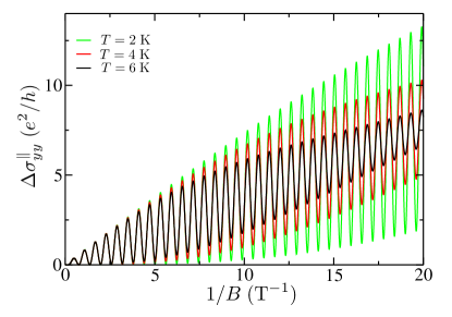
Figure 4: (Color online) Conductivity as a function of $1/B$ for the external in-plane magnetic field for different representative temperatures. Here we take $B_{\|}=8$T, $\lambda=100$nm, $h_{0}=1$nm, and $\tau\approx 10^{-13}$s.

Shubnikov de Haas (SdH) oscillations are also periodic in $1/B$. Since their periodicity does not depend on the profile heigh geometry, in principle, they are easy to distinguish from Weiss oscillations. Their characteristic temperatures are also very distinct: The temperature damping of the Weiss oscillations are given by Eq. (44) and the SdH characteristic temperature is Tan et al. (2011); Monteverde et al. (2010) $k_{B}T_{\rm SdH}=(\hbar\omega_{0}/2\pi^{2})(k_{F}l_{B})^{-1}$. Hence

$$\frac{T_{\rm W}}{T_{\rm SdH}}=\frac{k_{F}\lambda}{4}.$$ (60)

For the parameters we use $k_{F}\lambda\gg 1$, $T_{\rm W}/T_{\rm SdH}>1$. Thus, in general for a given temperature we expect the SdH oscillations to be more damped than the Weiss ones.

V Conclusions

We have studied the effects of a periodic profile height modulation on the electronic magnetotransport properties of graphene monolayer sheets. We have shown that such set up is suited for the study of Weiss oscillations either caused by strain fields or by an external magnetic field parallel to the graphene-substrate interface.

The Drude conductivity is obtained using first order perturbation theory within the effective low-energy Dirac Hamiltonian to calculate the semiclassical electronic velocity in the presence of a modulated potential. We built our analysis on the analytical results of Refs. Matulis and Peeters, 2007; Tahir and Sabeeh, 2008. We consider the cases of strain induced pseudo magnetic field and pseudo electric potential, as well as the case of a modulated effective magnetic field originated by an external $B$-field applied parallel to the graphene sheet. We studied the Weiss oscillations in the transverse conductivity in all these cases, discussing their geometry and temperature dependence. By casting the expressions for the conductivity in terms of the most relevant length scales of the problem we were able to verify that the classical interpretation of the Weiss oscillation based on the commensurability of the cyclotron orbit with the modulation period Beenakker (1989) still holds for Dirac-like Hamiltonian systems, a connection that has been so far overlooked in the graphene literature Tahir and Sabeeh (2008); Matulis and Peeters (2007); Tahir et al. (2007); Tahir and Sabeeh (2007).

We presented a careful discussion of the validity range of our theory taking into account realistic experimental values for the carrier concentration, modulation height profile and temperature. We stablished clear distinctions criteria between Weiss and Shubnikov de Haas oscillations, based on the behavior of the conductivity oscillations with doping, substrate height profile and temperature. Using these elements, we proposed a setup to experimentally investigate Weiss oscillations in graphene systems.

Such study can be particularly useful to provide further insight on effect of strain fields in the electronic properties of graphene, a subject of intense theoretical investigation, but still with limited quantitative experimental results.