Is state-dependent valuation more adaptive than simpler rules?

Abstract

McNamara, Trimmer, and Houston MTH12 claim to provide an explanation of certain systematic deviations from rational behavior using a mechanism that could arise through natural selection. We provide an arguably much simpler mechanism in terms of computational limitations, that performs better in the environment described by McNamara, Trimmer, and Houston MTH12. To argue convincingly that animals’ use of state-dependent valuation is adaptive and is likely to be selected for by natural selection, one must argue that, in some sense, it is a better approach than the simple strategies that we propose.

Acknowledgments:

This work was supported in part by NSF grants IIS-0911036 and CCF-1214844, by ARO grant W911NF-14-1-0017, by Simons Foundation grant #315783, and by the Multidisciplinary University Research Initiative (MURI) program administered by the AFOSR under grant FA9550-12-1-0040. Thanks to Arnon Lotem, Alex Kacelnik, and Pete Trimmer for their useful comments. Most of this work was carried out while the second author was at Harvard’s Center for Research on Computation and Society; Harvard’s support is gratefully acknowledged.

1 Introduction

Although much animal behavior can be understood as rational, in the sense of making a best response in all situations, some systematic deviations from rationality have been observed. For example, Marsh, Schuck-Paim, and Kacelnik MSK04 presented starlings with two potential food sources, one which had provided food during “tough times”, when the birds had been kept at low weight, while other had provided food during “good times”, when the birds were well fed. They showed that the starlings preferred the food source that had fed them during the tough times, even when that source had a longer delay to food than the other source. Similar behavior was also observed in fish and desert locusts [Aw, Holbrook, de Perera, and KacelnikAw et al.2009, Pompilio, Kacelnik, and BehmerPompilio et al.2006].

McNamara, Trimmer, and Houston MTH12 claim to provide an explanation of this behavior using a mechanism that could arise through natural selection. They provide an abstract model of the bird-feeding setting where a decision maker can choose either a “risky” action or a “safe” action. They also provide a mechanism that takes internal state into account and can lead to good results (where, in the example above, the internal state could include the fitness of each source). However, as we observe, for the particular parameters used in their model, there is a much better (in the sense of getting a higher survival probability) and much simpler approach than their mechanism that does not take the internal state into account: simply playing safe all the time. It is hard to see how the mechanism proposed by McNamara et al. could arise in the model that they use by natural selection; the simpler mechanism would almost surely arise instead.

The fact that always playing safe does well depends on the particular parameter settings used by McNamara et al. Playing safe would not be a good idea for other parameter settings. However, we show that a simple $2$-state automaton that more or less plays according to what it last got also does quite well. It does significantly better than the McNamara et al. mechanism, and does well in a wide variety of settings. Although our automaton also takes internal state into account (the internal state keeps track of the payoff at the last step), it does so in a minimal way, which does not suffice to explain the irrational behavior observed.

It seems to us that to argue convincingly that the type of mechanism proposed by McNamara et al. is adaptive, and is likely to be selected for by natural selection, and thus explains animals’ use of state-dependent valuation, then one must argue that, in some sense, it is a better approach than the simple strategies that we propose. Now it could be that the simple strategies we consider do not work so well in a somewhat more complicated setting, and in that setting, taking the McNamara et al.’s approach does indeed do better. However, such a setting should be demonstrated; it does not seem easy to do so. In any case, at a minimum, these observations suggest that McNamara et al.’s explanation for the use of state-dependent strategies is incomplete.

We should add that we are very sympathetic to the general approach taken by McNamara et al., although our motivation has come more from the work of Wilson W02 and Halpern, Pass, and Seeman HPS12,HPS13, which tries to explain seemingly irrational behavior, this time on the part of humans, in an appropriate model. That work assumes that people are resource-bounded, which is captured by modeling people as finite-state automata, and argues that an optimal (or close to optimal) finite-state automaton will exhibit some of the “irrational” behavior that we observe in people. (The $2$-state automaton that we mentioned above is in fact a special case of a more general family of automata considered in [Halpern, Pass, and SeemanHalpern et al.2012]; see Section 3.3.) We believe that taking computational limitations seriously might be a useful approach in understanding animal behavior, and may explain at least some apparently irrational behavior.

The rest of this paper is organized as follows. In Section 2, we review the model used by McNamara et al. MTH12 and compare it to that of [Halpern, Pass, and SeemanHalpern et al.2012]. In Section 3, we describe four strategies that an agent can use in the McNamara et al. model, under the assumption that the agent knows which action is the risky action and which is the safe action. One is the strategy used by McNamara et al.; another is a simplification of the strategy that we considered in our work; the remaining two are baseline strategies. In Section 4, we evaluate the strategies under various settings of the model parameters. In Section 5, we consider what happens if the agent does not know which action is risky and which is safe and, more generally, the issue of learning. We conclude in Section 6.

2 The model

McNamara et al. MTH12 assume that agents live at most one year, and that each year is divided into two periods, winter and summer. Animals can starve to death during a winter if they do not find enough food. If an agent survives the winter, then it reproduces over the summer, and reproductive success is independent of the winter behavior.

A “winter” is a series of $T$ discrete time steps. At any given time, the environment is in one of two states: $G$ (good) or $S$ (sparse); the state of the environment is hidden from the agent. At every time step there is a small probability $z$ of the environment switching states. At each time step, there are two actions potentially available to the agent, $A$ (which we think of as the “risky” action) or $B$ (the “safe” action). (The names “safe” and “risky” are due to the fact that the reward swings, depending on whether the environment is good or scarce, are greater for $A$ than for $B$.) With probability $\gamma$, both options are available to the agent; with probability $(1-\gamma)/2$, the agent must play $A$; and with probability $(1-\gamma)/2$, the agent must play $B$. The payoff of actions $A$ and $B$ depends on whether the state of the environment is $G$ or $S$.

An agent has a certain level of “energy reserves”, denoted by an integer between 0 and 10. The maximum level of energy reserves is thus 10; an agent dies if his energy-reserve level is $0$. At each time step, one unit of energy reserves is consumed. At each time step, an agent receives $0,1$ or $2$ units of energy. The probability of each of these amounts is drawn from a binomial distribution $bin(2,p)$ (so that the probability of receiving 0 units is $(1-p)^{2}$, the probability of receiving 1 unit is $2p(1-p)$, and the probability of receiving 2 units is $p^{2}$), where $p$ depends on the current environment state and the choice of action. $P_{GA}$ is used to denote the probability $p$ when the environment is in state $G$ and the agent plays action $A$; we can similarly define $P_{GB}$, $P_{SA}$, and $P_{SB}$. McNamara et al. assume that rewards are higher in expectation in the good environment for both actions, that is, $P_{GA}\geq P_{SA}$ and $P_{GB}\geq P_{SB}$); moreover, $A$ is the better action in the good environment, while $B$ is better in the sparse environment, so $P_{GA}\geq P_{GB}$ and $P_{SB}\geq P_{SA}$.

It is interesting to compare this model to that used by Halpern, Pass, and Seeman HPS12. Although, we mentioned in the introduction, their goal was to study irrational behavior in humans, and the kinds of behaviors considered were quite different from those considered by McNamara et al. (the focus was on modeling the behavior in game playing reported by Erev, Ert, and Roth erev2010entry), the models are surprisingly similar. The main differences between the two models is that, in the model of [Halpern, Pass, and SeemanHalpern et al.2012], an agent’s objective is to maximize his expected average payoff over rounds (rather than just to maximize the probability of surviving for a year). Agents never die; and an agent’s utility is taken to be the limit of his average reward per round over an infinite time horizon. In the language of McNamara, Trimmer, and Houston, Halpern, Pass, and Seeman take $\gamma=1$, so that both actions are always available. Moreover, instead of observing the payoff (which is deterministically dependent on the state of the world), an agent gets a signal correlated with the real state of the environment when he plays $A$, and no signal when he plays $B$. As discussed by Halpern et al. HPS12, getting a noisy payoff as in the McNamara et al. MTH12 model has essentially the same effect as getting a signal correlated with the environment’s state. As we discuss later, in the scenarios we study here, $P_{GB}$ and $P_{SB}$ are very close and thus the signal we get about the environment by playing $B$ is very weak in this model as well.

3 Four Strategies

In this section, we describe four strategies that an agent can use in the McNamara et al. model. We will be interested in the probability that an agent survives a “winter” period using each of these strategies. Note that the higher this probability is, the greater the probability that this strategy will emerge as the dominant strategy in an evolutionary process.

3.1 Baseline strategies

We consider two baseline strategies. The first is called the oracle strategy. With this strategy, we assume that an agent knows the true state of the environment before choosing his action, and thus can make the optimal choice in each round. While this strategy cannot be implemented by an agent in this model, we use it to provide an upper bound on the the survival probability of the agent. Clearly, no strategy can do better than the oracle strategy.

The second baseline strategy we consider is the safe strategy. With the safe strategy, the agent always plays the safe action ($B$) when that choice is available (recall that in some rounds the agent is forced to play $A$).

3.2 The value strategy

The strategy studied by McNamara et al. MTH12, which we call the value strategy, is based on keeping a value $V(\cdot)$ for each of the actions and choosing the action with the highest value in each round. This value is updated in every round using the formula $V_{new}=(1-\beta)V_{old}+\beta w$, where $\beta$ is a fixed parameter controlling the learning rate and $w$ is the perceived reward, which is defined in more detail below.

In a little more detail, $V(i)$ is initialized to the expected energy reward of action $i$. In a round where action $i$ is performed, $V(i)$ is updated using the formula above (taking $V_{old}(i)$ to be the currently stored value of $V(i)$ and $V_{new}(i)$ to be the updated value), where $w=ue^{k(r-5)}$, $u$ is the number of energy units received as a result of performing action $i$, $r$ is the current reserve level, and $k$ is a fixed constant that might evolve to match the scenario parameters.

In a round where the agent can play both $A$ and $B$ (which will be the case with probability $1-\gamma$), it plays whichever one has higher value. That is, it plays $A$ if $V(A)\geq V(B)$, and otherwise plays $B$.

3.3 The automaton strategy

The last strategy we consider is inspired by the strategy used by Halpern, Pass, and Seeman HPS12; we call it the automaton strategy. With the automaton strategy, an agent keeps an internal state that is correlated with the number of good and bad signals it has seen recently. Thus, the internal state is not determined by the agent’s internal reserves, but rather by recent observations. This strategy is described by a finite automaton with $n$ states denoted $[0,\ldots,n-1]$. If the automaton has a choice, then it plays action $B$ (the “safe” action) in state 0 and plays action $A$ in all the remaining states. (Thus, if the automaton has only one state, it plays the safe strategy.) The automaton changes state depending on the signal it observes. Halpern, Pass, and Seeman assumed that an automaton in state $0\leq i<n$ moved to $i+1$ with probability $p_{up}$ whenever it received a signal that was highly correlated with the environment being in state $G$; an automaton in state $i>0$ moved to state to $i-1$ with probability $p_{down}$ whenever it receives a signal that was highly correlated with the environment being in state $S$; and an automaton in state 0 (which never received a signal that would cause it to move in our earlier work, since it always played $B$) moved to state 1 with a small “exploration” probability $p_{exp}$. If an automaton did not change state according to the rules above, it just remains in the same state.

For the purposes of this paper, we take “received a signal highly correlated with environment being in state $G$” to mean “played $A$ and got a reward of 2”; while “received a signal highly correlated with the environment being in state $S$” means “played $A$ and got a reward of 0”. (We justify these choices in the next section.) For simplicity, we take $p_{up}=p_{down}=1$ and $p_{exp}=0$, so that the automaton is deterministic. Note that we are able to take $p_{exp}=0$ because $\gamma<1$, so that even in state 0, the automaton will play $A$ with probability $(1-\gamma)/2$. (McNamara et al. MTH12 also point out that randomization is useful when $\gamma=1$.)

4 Evaluating the Strategies

In this section we evaluate the four strategies discussed in the previous section under various settings of the model parameters. We calculate the survival probability of an agent using the strategy over a winter of length $T=500$ steps by simulating $100000$ winters and looking at the ratio of runs in which the agent survived. We initialize the environment to the sparse state and the resource level to the maximum of $10$.

4.1 Using the McNamara et al. parameter settings

We first study the performance of these strategies using the baseline parameter setting considered by McNamara et al. MTH12: the environment changes with probability $z=0.02$ at each round; the payoffs are $P_{GA}=0.9,P_{GB}=0.7,P_{SA}=0.4,P_{SB}=0.6$; and $\gamma=0.5$, so half the time, an agent has both options available, one quarter of the time, $A$ must be played, and one quarter of the time, $B$ must be played. Note that with these parameter settings, when playing $B$, the expected gain in energy reserves is very close if the environment is in state $S$ and in state $G$. Thus, the agent does not learn much about the state of the environment when playing $B$. Thus, these parameter settings lead to a situation similar to that in [Halpern, Pass, and SeemanHalpern et al.2012], where it is assumed that the agent gets no information when it plays $B$. On the other hand, there is a significant gap in the expected gain in energy reserves between $P_{SA}$ and $P_{GA}$, so the agent can make useful inferences about the state of the environment based on its reward when it plays $A$.

According to McNamara et al, these parameter settings were chosen to ensure a high survival probability. Indeed, our baseline oracle strategy has a survival probability of roughly $91\%$. With McNamara et al.’s parameter settings, an animal has an expected positive gain of energy resources in each round, even though it is forced to play $B$ one quarter of the time. In the good environment it gets an even larger expected gain in energy resources and thus gets to its maximum level with high probability. Thus, its survival probability is high, although it might still die even with this strategy.

With these parameter settings, McNamara et al. found that the value strategy performed best with the constant $k$ used in evaluating $w$ set to $-.2$, so we used this value in our experiments; we also follow McNamara et al. in taking the parameter $\beta$ to be $.02$. With these settings, the value strategy has a survival probability of just below $80\%$ (which matches the findings in McNamara et al. MTH12). Note that the negative value of $k$ says that the strategy gives greater perceived value for a reward received when its resource are low. McNamara et al. view this as a justification for animals preferring option $B$.

Although the value strategy does well, the safe strategy does even better. Indeed, its survival rate is almost 91%, that is, just about as good as that of the oracle strategy. This is actually straightforward to check analytically as well. It is not hard to explain the good performance of the safe strategy compared to the oracle strategy. In the sparse environment it plays exactly as the oracle strategy, while in the good environment, since the expected return at each step even when playing $B$ is high, it reaches the limit of $10$ units with high probability by playing $B$; playing $A$ has no real advantage.

For the same reasons, the automaton strategy also performs significantly better than the value strategy. An automaton with only 2 states and with deterministic transitions (so $p_{up}=p_{down}=1$) has a survival probability of over 85%. Adding more states to the automaton did not help with this setting of the model parameters.

We tested the strategies with different lengths of winter, ranging from $100$ to $1000$ steps, to see how robust these outcomes are. For the value strategy we tested $3$ different values of $k$, since McNamara et al. MTH12 found that different optimal values evolve for different winter lengths. We compare the performance of all three, as well as just the maximum of them with all other strategies. As can be seen in Figure 1, the safe strategy consistently perform as well as the oracle strategy. Also, the automaton strategy performs consistently better than the value strategy, even with only 2 states and compared to the best choice of $k$ for each choice of $T$, and the gap increases as $T$ grows.

The reason that the value strategy underperforms in these settings is that although there is no real advantage to playing $A$, after a long period of the environment being in state $G$, the value strategy sticks with $A$ for a while, which puts it at risk when the environment switches to $B$. (The same is true for automata with extra states.)

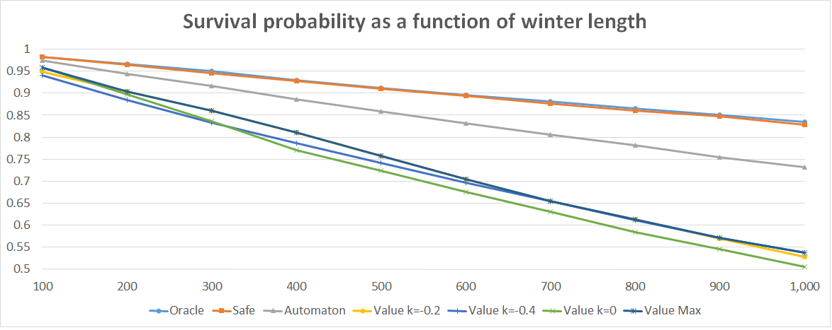
Figure 1: Survival probability with different winter lengths

4.2 Being safe is not always better

While the safe strategy performed just about as well as the optimal oracle strategy for the parameter settings used by McNamara et al., it did not do as well for other parameter settings. Recall that the safe strategy is just the automaton strategy with one state, which can be viewed as saying that while an automaton can get away with being “dumb” for the parameter settings considered by McNamara et al., there exist environment conditions where more states are desirable. In particular, this happens when the expected payoff of playing $B$ drops and $\gamma$ gets closer to $1$, so that the agent is not forced to play $A$ in many rounds.

For example, when $P_{GA}=0.8,P_{GB}=0.55,P_{SA}=0.3,P_{SB}=0.55$ (note that the expected value of both actions is the same) and $\gamma=0.9$ we get that the survival probability of the automaton strategy with $2$ states is $\sim\,74\%$ while the safe strategy only gives $\sim\,70\%$ (the oracle strategy has $\sim\,86\%$ survival probability). This gap grows as $T$ grows. The value strategy performs quite badly with these parameter settings; it leads to a survival probability of only $\sim\,5\%$ (for the best choice of $k$).

It is not hard to explain these results. In these settings, the reward from playing $B$ is not enough to guarantee survival with high probability, so the automaton strategy gains from being able to play $A$. In addition, the reward from $A$ is a very good signal of the state of the environment, so the automaton strategy does not keep playing $A$ for too long when it should not. The value strategy does not do so well in this case, since playing $A$ in the sparse environment is quite bad, while when the environment is in a good state, the value of $A$ becomes much higher than that of $B$, which makes it slow to switch. As both actions are available in most rounds, this leads to a low probability of survival for the value strategy.

Having more than two states becomes more useful when playing $B$ is bad in the good environment (i.e., $P_{GB}<0.5$) and the signal from playing $A$ is not very strong (i.e., $P_{SA}$ and $P_{GA}$ are not too far apart). Note however, that these condition are outside the scope of parameters allowed by the model specified by McNamara et al. MTH12 (as $P_{GB}<P_{SB}$ if we want a good payoff for $B$ in the sparse environment).

5 Discussion

While we show that the automaton strategy is better than the value strategy in many scenarios, as we discussed before, the value strategy (or, more generally, state-dependent strategies), seem to be what animals actually use in the scenarios studied in previous papers. We now discuss some possible explanations for this.

5.1 The learning challenge

One advantage of the value strategy is that it does not need to “understand” that $A$ is the “risky” action and $B$ is the “safe” action. It just calculates a value for each strategy and plays the strategy with the higher value. By way of contrast, there is a sense in which the safe strategy and the automaton strategy need to understand beforehand that $B$ is safe. As long as roles are reasonably stable (over evolutionary timescales), this is not a problem; evolutionary pressures would result in animals effectively learning which actions are safe and which are risky. And if roles change over time, then again we would expect mutations to survive that switched the role of $A$ and $B$, provided that the change is sufficiently slow.

What happens in new environments where the animal does not initially know which actions are safe or in environments where the roles of “safe” and “risky” actions change relatively frequently? It is easy to extend the automaton strategy by adding a “front end”, so to speak, that keeps learning which action is safe and which is risky. For example, the agent can keep track of the payoffs in the last $m$ rounds (for a small value of $m$, say 10-15) to see if they are in line with the current choices of safe and risky actions; if not, the choices of “safe” and “risky” can be switched. If the payoff difference between the safe and risky strategies is relatively large (in at least one state), then this can be learned quickly; if it not so large, then it does not matter so much which action is performed.

It also worth noting that the value strategy also has some parameters ($\beta$ and $k$) that might depend on the environment and require some learning process. These observations suggest that learning by itself is not the explanation for the usage of the value strategy by animals.

5.2 A hybrid strategy

Another possible explanation is that animals use a hybrid strategy, combining features of both the value strategy and the automaton strategy. The value strategy seems to do well in learning the value of actions in a new environment and reacting to changes in the value of actions themselves. However, the automaton strategy is better at tracking the current environment and reacting to somewhat periodic changes in the environment. The use of a hybrid strategy is supported by the fact that the animal’s preference for food sources presented during tough times is ephemeral; as soon as animals experience both sources in the same state, they start switching preference to the option with higher resource payoff [Alex Kacelnik, private communication, 2016]. Thus, when the environment stabilizes, animals might be switching from a state-dependent strategy to using the “safe” strategy. Of course, more research is needed to see if this is what actually happens.

6 Conclusion

Our results show that some very simple strategies seem to consistently outperform the value strategy. This gap grows as the task of surviving becomes more challenging (either because “winter” is longer or the rewards are not as high). This at least suggests that the model considered by McNamara et al. MTH12 is not sufficient to explain the evolution of the value strategy in animals. McNamara et al. claim that “[w]hen an animal lacks knowledge of the environment it faces, it may be adaptive for the animal to base its decision upon approximate cues.” We are very sympathetic to this claim, although we have argued that it may be more useful for those cues to include recent evidence about rewards, not just the internal food state, at least for the parameter settings considered by McNamara et al. It would be interesting to understand better how the interaction of cues is used by animals.

References

- [\citeauthoryearAw, Holbrook, de Perera, and KacelnikAw et al.2009] Aw, J. M., R. I. Holbrook, T. B. de Perera, and A. Kacelnik (2009). State-dependent valuation learning in fish: Banded tetras prefer stimuli associated with greater past deprivation. Behavior Processes 81, 333–336.
- [\citeauthoryearErev, Ert, and RothErev et al.2010] Erev, I., E. Ert, and A. E. Roth (2010). A choice prediction competition for market entry games: An introduction. Games 1, 117–136.
- [\citeauthoryearHalpern, Pass, and SeemanHalpern et al.2012] Halpern, J. Y., R. Pass, and L. Seeman (2012). I’m doing as well as I can: modeling people as rational finite automata. In Proc. Twenty-Sixth National Conference on Artificial Intelligence (AAAI ’12).
- [\citeauthoryearHalpern, Pass, and SeemanHalpern et al.2014] Halpern, J. Y., R. Pass, and L. Seeman (2014). Decision theory with resource-bounded agents. Topics in Cognitive Science 6(2), 245–257.
- [\citeauthoryearMarsh, Schuck-Paim, and KacelnikMarsh et al.2004] Marsh, B., C. Schuck-Paim, and A. Kacelnik (2004). Energetic state during learning affects foraging choices in starlings. Behavioral Ecology 15, 396–399.
- [\citeauthoryearMcNamara, Trimmer, and HoustonMcNamara et al.2012] McNamara, J. M., P. C. Trimmer, and A. I. Houston (2012). The ecological rationality of state-dependent valuation. Psychological review 119(1), 114.
- [\citeauthoryearPompilio, Kacelnik, and BehmerPompilio et al.2006] Pompilio, L., A. Kacelnik, and S. T. Behmer (2006). State-dependent learned valuation drive choice in an invertebrate. Science 311, 1613–1615.
- [\citeauthoryearWilsonWilson2015] Wilson, A. (2015). Bounded memory and biases in information processing. Econometrica 82(6), 2257–2294.