Coulomb-blockade and Pauli-blockade magnetometry

Abstract

Scanning-probe magnetometry is a valuable experimental tool to investigate magnetic phenomena at the micro- and nanoscale. We theoretically analyze the possibility of measuring magnetic fields via the electrical current flowing through quantum dots. We characterize the shot-noise-limited magnetic-field sensitivity of two devices: a single dot in the Coulomb blockade regime, and a double dot in the Pauli blockade regime. Constructing such magnetometers using carbon nanotube quantum dots would benefit from the large, strongly anisotropic and controllable g tensors, the low abundance of nuclear spins, and the small detection volume allowing for nanoscale spatial resolution; we estimate that a sensitivity below $1\,\mu\text{T}/\sqrt{\text{Hz}}$ can be achieved with this material. As quantum dots have already proven to be useful as scanning-probe electrometers, our proposal highlights their potential as hybrid sensors having in situ switching capability between electrical and magnetic sensing.

I Introduction

The detection of weak magnetic fields with high spatial resolution is a task of great importance in diverse areas, from fundamental physics and chemistry to practical applications in data storage and medical imaging. This task can be tackled by scanning-probe magnetic-field sensors, based on various operating principlesBending (1999); Martin and Wickramasinghe (1987); Chang et al. (1992); Kirtley et al. (1995); Allred et al. (2002); Rugar et al. (2004); Taylor et al. (2008); Milde et al. (2013); Switkes et al. (1998); Lassagne et al. (2011). Low-temperature scanning-probe magnetometry has been successfully used to image a range of nontrivial magnetic phenomena, e.g., vortices in superconductorsKirtley et al. (1996); Pelliccione et al. (2016); Thiel et al. (2016), exotic magnetic structuresMilde et al. (2013); Kezsmarki et al. (2015); Wang et al. (2015), and current-induced magnetic fields in various systemsBluhm et al. (2009); Kalisky et al. (2013) including topological insulatorsSpanton et al. (2014); Nowack et al. (2013). The applicability of the different magnetic-field sensors (SQUIDs, Hall bars, NV centers, etc) for specific tasks is determined by a number of characteristics, including magnetic-field sensitivity and detection volume, the latter one related to the achievable spatial resolution. A key challenge is to improve the capabilities of these sensors, either by advancing existing designs, or by devising completely new principles and devices.

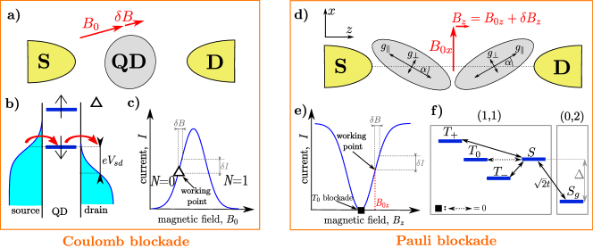
Figure 1: (Color online) Coulomb-blockade and Pauli-blockade magnetometry. (a) Coulomb-blockaded single-level quantum dot between source (S) and drain (D). The spin states are split by an offset magnetic field $B_{0}$ setting the working point. (b,c) Current is flowing through the $\downarrow$ state, therefore the current changes by $\delta I$ if the energy of $\downarrow$ is changed by a small variation $\delta B$ of the magnetic field. This allows for measuring $\delta B$ via measuring the current. The shaded areas in (b) represent the thermally broadened electronic Fermi-Dirac distributions in the contacts. (d) Pauli-blockaded double quantum dot. The two ellipsoids represent the $g$-tensors on the two dots. The $g$-tensors are anisotropic, and have misaligned principal axes in the two dots, enclosing the misalignment angle $2\alpha$. The working point of the magnetometer is set by the field $\text{\boldmath{$B$}}_{0}=(B_{0x},0,B_{0z})$, and $\delta B_{z}$ is measured via measuring the change $\delta I$ [see (e)] in the current flowing through the dots. (e) Current as a function of $B_{z}$. Black square ($\blacksquare$) denotes the point of $T_{0}$ blockade. (f) Two-electron level diagram in the vicinity of $T_{0}$ blockade. Solid and dotted black arrows represent magnetic-field-induced coupling matrix elements. At the $T_{0}$ blockade ($\blacksquare$), the $T_{0}$-$S$ coupling (dotted black arrow) vanishes.

In this work, we propose and theoretically explore two quantum-dot-based low-temperature approaches to magnetic-field sensing, offering a combination of sub-$\mu\textrm{T}/\sqrt{\textrm{Hz}}$ magnetic-field sensitivity, nanoscale spatial resolution, and conceptual simplicity via all-electrical and all-dc operation (i.e., optical or high-frequency electronic elements are not required). In both devices, the magnetic field is measured by measuring the electric current through the dots. The first, simpler device we study is a single quantum dot in the Coulomb blockade regime; the second one is a double quantum dot (DQD) in the Pauli blockade regimeOno et al. (2002). Our main goal is to determine the fundamental limits on the achievable magnetic-field sensitivity of these sensors by considering the effects of shot noise and the thermal broadening of the electron distributions in the contacts. We also discuss the effect of electric potential fluctuations on the sensitivity, and highlight the advantages of carbon nanotubes (CNTs) for realizing the proposed magnetometry principle.

II Sensitivity of a current-based magnetometer

Before presenting the concrete magnetometry schemes, we first characterize the shot-noise-limited sensitivity of a generic magnetometer that is based on the magnetic-field dependence $I(\text{\boldmath{$B$}})$ of the steady-state electric current flowing through a mesoscopic conductor. We wish to exploit this dependence for measuring small deviations $\delta\text{\boldmath{$B$}}$ of the magnetic field from a pre-set ‘offset field’ or ‘working point’ $\text{\boldmath{$B$}}_{0}$. We focus on the generic situation when the current is linearly sensitive to a single Cartesian component of $\delta\text{\boldmath{$B$}}$, say, $\delta B_{z}$; that is, $I^{\prime}(\text{\boldmath{$B$}}_{0})\equiv\left.\frac{\partial I}{\partial B_{z}}\right|_{\text{\boldmath{$B$}}_{0}}>0$, and $\left.\frac{\partial I}{\partial B_{x}}\right|_{\text{\boldmath{$B$}}_{0}}=\left.\frac{\partial I}{\partial B_{y}}\right|_{\text{\boldmath{$B$}}_{0}}=0$. This is always fulfilled if we align the $z$ axis with the gradient vector of $I(\text{\boldmath{$B$}})$ at $\text{\boldmath{$B$}}_{0}$. In this case, the device can be operated as a linear detector of $\delta B_{z}$. In analogy with the sensitivity formula for a current-based electrometerKorotkov et al. (1992), we claim that the magnetic-field sensitivity of the magnetometer is characterized by the quantity

$$S(\text{\boldmath{$B$}}_{0})=\frac{\sqrt{eF(\text{\boldmath{$B$}}_{0})I(\text{\boldmath{$B$}}_{0})}}{I^{\prime}(\text{\boldmath{$B$}}_{0})},$$ (1)

where $e$ is the absolute value of the electron’s charge, and $F$ is the Fano factorBlanter and Büttiker (2000), defined as the ratio of the shot noise and the current. For more details, see Appendix A. In what follows, we will refer to the shot-noise-limited sensitivity $S$ as the sensitivity.

The dimension of $S$ is ${\rm T}/\sqrt{\rm Hz}$. A smaller value of $S$ implies the ability of resolving smaller differences in $\delta B_{z}$ in a given measurement time window; that is, an improved performance. Equation (1) is in line with the expectation that the sensitivity is improved if the noise is suppressed ($F$ is decreased) or if the dependence of the current on the magnetic field is enhanced ($I^{\prime}(\text{\boldmath{$B$}}_{0})$ is increased).

III Coulomb-blockade magnetometry

Here, we describe and characterize a principle of magnetometry based on Zeeman-splitting-induced changes in the current flowing through a single dot, as sketched in Fig. 1a,b,c. The scheme is analogous to the electrometer described in Refs. Korotkov et al., 1992; Korotkov, 1994.

The dot, shown schematically in Fig. 1a, is gate-voltage-tuned to the vicinity of a Coulomb peak, and a finite magnetic field $\text{\boldmath{$B$}}_{0}=(0,0,B_{0})$ creates a large Zeeman splitting $g\mu_{B}B_{0}$, where $g$ is the material-dependent effective $g$-factor of the electron. The Zeeman splitting separates the singly occupied $\uparrow$ (spin-up) excited state from the $\downarrow$ (spin-down) ground state, as shown in Fig. 1b. The magnetic field also creates a Zeeman splitting in the leads. We assume that under a finite source-drain bias voltage, the electron distributions in the leads are thermal (represented by the shaded regions in Fig. 1b) and are characterized by spin-independent local chemical potentials (represented as the dashed horizontal lines in Fig. 1b). A plunger gate voltage and a small source-drain bias voltage can be used to tune the energy levels such that $\downarrow$ is in the source-drain bias window as shown in Fig. 1b. Then the current flows via sequential tunneling through the transport cycle $0\to\downarrow\to 0$, where 0 corresponds to an empty dot, and $I(B_{0})$ is set to the slope of the Coulomb-peak, see the working point in Fig. 1c. Then, a small $\delta B$ increase in the $z$ component of the magnetic field lowers the energy of the current-carrying $\downarrow$ state by $g\mu_{B}\delta B$, and therefore increases the current flowing through the dot by the amount $\delta I$ as shown in Fig. 1c; measuring this increase $\delta I$ of the current will reveal $\delta B$.

This measurement scheme is directionally sensitive in the following sense. Assume that the small change in the magnetic field has all three Cartesian components, $\delta\text{\boldmath{$B$}}=(\delta B_{x},\delta B_{y},\delta B_{z})$, and it is much weaker than the offset field, $\delta B\ll B_{0}$. Then the Zeeman splitting $g\mu_{B}\sqrt{(B_{0}+\delta B_{z})^{2}+\delta B_{x}^{2}+\delta B_{y}^{2}}$ is well approximated by $g\mu_{B}\left(B_{0}+\delta B_{z}+\frac{\delta B^{2}}{2B_{0}}\right)$, that is, it is mainly determined by the component $\delta B_{z}$ along the offset field.

Now we use simple considerations to estimate the parameter dependence of the sensitivity $S$, and argue that the temperature has a strong influence on the optimal sensitivity: the latter is degraded as $T$ is increased. For these considerations, we introduce the characteristic rate $\Gamma$, describing the tunnel coupling of the dot to the source and drain leads. We propose that at a given $T$, (i) the sensitivity is optimized if $h\Gamma$ is comparable to $k_{B}T$, and (ii) the order of magnitude of the optimal sensitivity is estimated as

$$S_{\text{opt}}\sim\frac{\sqrt{hk_{B}T}}{g\mu_{B}}.$$ (2)

The reasoning is as follows. The height of the Coulomb peak is set by the lead-dot tunneling rate $\Gamma$, $I\sim e\Gamma$, whereas the Fano factor is $F\sim 1$. The slope of the Coulomb peak can be set by thermal broadening or tunnel broadening: $I^{\prime}\sim\frac{e\Gamma}{\max\{h\Gamma,k_{B}T\}/g\mu_{B}}$. Then, Eq. (1) implies $S\sim\frac{\max\{h\Gamma,k_{B}T\}}{g\mu_{B}\sqrt{\Gamma}}$. On the one hand, this has the consequence that for slow tunneling, $\Gamma<k_{B}T$, the sensitivity $S\propto 1/\sqrt{\Gamma}$ decreases with increasing $\Gamma$; on the other hand, for fast tunneling $\Gamma>k_{B}T$, the sensitivity $S\propto\sqrt{\Gamma}$ increases with increasing $\Gamma$. These imply claims (i) and (ii). Using the estimate in Eq. (2) and the values $g=30$, achievable in clean CNT dotsAjiki and Ando (1993); Minot et al. (2004); Kuemmeth et al. (2008); Laird et al. (2015), and $T=50\,\text{mK}$, we find $S_{\text{opt}}\sim 77\,\text{nT}/\sqrt{\text{Hz}}$.

Now we go beyond the previous estimate and quantify the magnetic-field sensitivity of the Coulomb-blockade magnetometry via a simple model. The single-electron Hamiltonian of the quantum dot involves the on-site energy $\epsilon$ and the Zeeman term: $H_{\text{CBM}}=\epsilon+\frac{1}{2}g\mu_{B}B\sigma_{z},$ where $g$ is the effective g factor, $\mu_{B}$ is the Bohr magneton, and $B$ is the magnetic field. The electronic Fermi-Dirac distributions in the source and drain leads are characterized by their common temperature $T$ and symmetrically biased chemical potentials $\mu_{L}=-\mu_{R}=eV_{sd}/2$ with $V_{sd}$ being the source-drain bias voltage. Lead-dot tunneling rates are set by the rate $\Gamma$, the level positions, and the Fermi-Dirac distributions of the leads. We describe the transport process by a classical master equation, neglecting double occupancy of the dot. The current $I$ and the Fano factor $F$ is evaluated using the counting-field methodBagrets and Nazarov (2003); Belzig (2005); details can be found in Appendix C. From these, the magnetic-field sensitivity $S$ is calculated from Eq. (1).

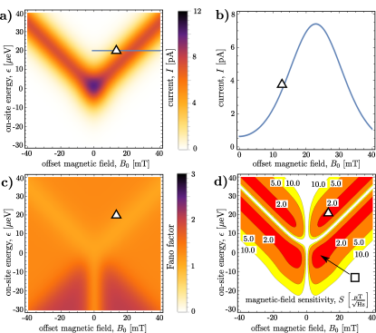
Figure 2: Coulomb-blockade magnetometry: Magnetic-field sensitivity of a single quantum dot. (a,b) Current, (c) Fano factor, and (d) sensitivity of a Coulomb-blockade magnetometer. (b) Magnetic-field dependence of the current along the blue line ($\epsilon=20\,\mu\text{eV}$) in (a). The white triangle $\triangle$ denotes a local minimum of the sensitivity $S$ along the blue line in (a). The optimal value of sensitivity denoted by the white square $\square$ is $S=1.4\ \mu\text{T}/\sqrt{\text{Hz}}$. Parameters: $V_{sd}=8.6\,\mu\text{V}$, $k_{B}T=4.3\,\mu\text{eV}$ ($T\approx 50$ mK), $h\Gamma=0.86\,\mu\text{eV}$ ($\Gamma\approx 200$ MHz, $e\Gamma\approx 33\,\text{pA}$), $g=30$.

Figures 2a,c,d shows the calculated current $I$, Fano factor $F$ and magnetic-field sensitivity $S$, respectively, as functions of the offset field $B_{0}$ and the on-site energy $\epsilon$ of the dot, for a given parameter set (see caption) where the thermal energy scale $k_{B}T$ dominates the tunneling energy scale $h\Gamma$. Figure 2b shows a horizontal cut of the current, $I(B_{0},\epsilon=20\,\text{meV})$, along the blue horizontal line in Fig. 2a. The dark spot in the centre of Fig. 2a, at $\epsilon\approx 0$ and $B_{0}\approx 0$, is a finite-bias Coulomb peak, where the two spin levels $\downarrow$ and $\uparrow$ are approximately degenerate, both of them is located within the bias window, and hence both contributes to the current. The dark diagonal lines forming the V-shaped region in Fig. 2a correspond to Coulomb peaks where the current is carried by a single spin level, as shown in Fig 1b: a Zeeman splitting $g\mu_{B}B_{0}>k_{B}T,eV_{sd}$ exceeding the thermal and voltage broadening is induced between the spin levels by the offset field $B_{0}$, thereby only the lower-energy spin level contributes to the current.

The typical values of the Fano factor in Fig. 2c corroborate our above estimate $F\sim 1$, and implies that the Fano factor plays a minor role in determining the order of magnitude of the magnetic-field sensitivity. The sensitivity in Fig. 2d is therefore following a pattern which can essentially be deduced from the pattern of the current, Fig. 2a: the sensitivity is good, that is, $S$ is small, wherever the derivative of the current with respect to the offset field is appreciable; that is, along the two slopes of the V-shaped high-current regions of Fig. 2a. In Fig. 2d, the sensitivity has a local minimum $S=1.7\,\mu\text{T}/\sqrt{\text{Hz}}$ at the white triangle.

Note that in Fig. 2d, the global minimum of the magnetic-field sensitivity is at the working point marked by the white square ($\square$), which corresponds to $(\epsilon,B_{0})\approx(0\ \mu\text{eV},10\ \text{mT})$. At $\square$, the value of the sensitivity is $S=1.4\ \mu\text{T}/\sqrt{\text{Hz}}$. We emphasize that the operation of the magnetometer at this working point $\square$ is not following the scheme that we outlined above and visualized in Fig. 1b. The scheme of operation in the working point $\square$ is discussed in detail in Appendix B. In Appendix B, we also argue that by choosing an appropriate working point in the vicinity of $\square$, the sensitivity-degrading effects of electric potential fluctuations can be mitigated.

To conclude, we argued that the fundamental limit on the magnetic-field sensitivity of a Coulomb-blockade magnetometer is set by the temperature, evaluated and analyzed the magnetic-field sensitivity of such a device using a simple model, and estimated that at experimentally available low temperatures, and with a large g-factor, e.g., offered by CNT dots, the optimal magnetic-field sensitivity can be below $\mu\text{T}/\sqrt{\text{Hz}}$.

IV Pauli-blockade magnetometry

Here, we describe an alternative magnetometer based on a DQD operated in the Pauli blockade regimeOno et al. (2002). In such DQDs, the magnetic-field dependence of the current can be caused by various mechanisms, e.g., hyperfine interactionKoppens et al. (2005); Jouravlev and Nazarov (2006) or spin-orbit interactionPfund et al. (2007); Danon and Nazarov (2009). Here, we focus on one particular mechanism, where the magnetic-field dependence of the current is governed by the different and strongly anisotropic g-tensors in the two dots, as depicted in Fig. 1d. We will show that if we have this feature in the device, then the magnetic-field sensitivity is optimized in the close vicinity of a special setting that we call the ‘$T_{0}$ blockade’ (see Fig. 1e,f, and below). Based on a comparison of a recent experimentPei et al. (2012) and our corresponding theoretical resultsSzéchenyi and Pályi (2015), we argue that DQDs in bent CNTs provide an opportunity to meet these requirements.

In the Pauli-blockade regime, a large dc source-drain voltage is applied to a serially coupled DQD, and a dc current might flow via the transport cycle $(0,1)\rightarrow(1,1)\rightarrow(0,2)\rightarrow(0,1)$, where ($N_{L}$, $N_{R}$) denotes the number of electrons in the left and right dots. The $(1,1)\rightarrow(0,2)$ transition is blocked due to Pauli’s exclusion principle if a (1,1) triplet state becomes occupied during the transport process, leading to a complete suppression of the current. We describe the DQD by the two-electron HamiltonianJouravlev and Nazarov (2006) $H=H_{B}+H_{\textrm{tun}}+H_{\Delta}$. The interaction of the external homogeneous magnetic field and the electron spins is

$$H_{B}=\frac{1}{2}\mu_{B}\text{\boldmath{$B$}}\cdot\left({\mathbf{\hat{g}}}_{L}\boldsymbol{\sigma}_{L}+{\mathbf{\hat{g}}}_{R}\boldsymbol{\sigma}_{R}\right).$$ (3)

Here, $\boldsymbol{\sigma}_{L/R}$ is the vector of Pauli matrices representing the spins of the electrons. The $g$-tensors $\mathbf{\hat{g}}_{L}$ and $\mathbf{\hat{g}}_{R}$ are assumed to have the same principal values $g_{\perp}$, $g_{\perp}$, $g_{\parallel}$ in the dots $L$ and $R$. (This is not a strict requirement, as we discuss in section V.4.) Furthermore, the principal axes of the g-tensors enclose a small angle $2\alpha\ll 1$, as shown in Fig. 1d. Choosing the coordinate system as depicted in Fig. 1d, the $g$-tensors are given as $\mathbf{\hat{g}}_{D}=g_{\parallel}\text{\boldmath{$t$}}_{D}\circ\text{\boldmath{$t$}}_{D}+g_{\perp}\left(1-\text{\boldmath{$t$}}_{D}\circ\text{\boldmath{$t$}}_{D}\right),$ where $\text{\boldmath{$t$}}_{D}=(D\sin\alpha,0,\cos\alpha)$ is the unit vector pointing along the local principal axis of $g_{\parallel}$ in dot $D\in(L,R)\equiv(-1,1)$. Spin-conserving tunneling between the dots is represented by $H_{t}=\sqrt{2}t(|S_{g}\rangle\langle S|+|S\rangle\langle S_{g}|)$, where $S$ [$S_{g}$] is the singlet state in the (1,1) [(0,2)] charge configuration. The last term $H_{\Delta}=-\Delta|S_{g}\rangle\langle S_{g}|$ describes the energy detuning between the (1,1) and (0,2) charge configurations. Finally, the incoherent tunneling processes from the source electrode to dot $L$ (from dot $R$ to the drain electrode) are characterized by the rate $\Gamma_{L}$ ($\Gamma_{R}$).

In this model, the $T_{0}$ blockade appears in the case when the magnetic field is aligned with the $x$ axis, $\text{\boldmath{$B$}}=(B,0,0)$. Then, taking the spin quantization axis along $x$, which coincides with the direction of $B$ as well as with that of the average effective magnetic field $\frac{1}{2}\left(\mathbf{\hat{g}}_{L}+\mathbf{\hat{g}}_{R}\right)\text{\boldmath{$B$}}$, the (1,1) triplet state $|T_{0}\rangle=\frac{1}{\sqrt{2}}\left(|\uparrow\downarrow\rangle+|\downarrow\uparrow\rangle\right)$ is an energy eigenstate, implying that it is decoupled from the (0,2) charge configuration and therefore blocks the current Jouravlev and Nazarov (2006). This setting is indicated in Fig. 1e and f by the black square ($\blacksquare$). The other four two-electron energy eigenstates all contain a finite (0,2) component and therefore can decay to the single-electron states by emitting an electron to the drain; hence we call this special case the $T_{0}$ blockade. Note that the appearance of the $T_{0}$ blockade does not require the equality of the g-tensor principal values in the two dots, see section V.4.

Importantly, the $T_{0}$ blockade is maintained as long as the magnetic field lies in the $xy$ plane. It is however lifted by a finite $B_{z}$ component, as the latter couples $T_{0}$ to the singlet states Jouravlev and Nazarov (2006). Therefore, in the vicinity of the $T_{0}$ blockade, the current is mostly determined by $B_{z}$. The decay rate of $\bar{T}_{0}$, that is, the energy eigenstate that evolves from $T_{0}$ as $B_{z}$ is turned on, is given by $\bar{\Gamma}=2\Gamma_{R}\left|\langle S_{g}|\bar{T}_{0}\rangle\right|^{2}$. We express $\bar{T}_{0}$ using first-order perturbation theory in $\mu_{B}g_{\parallel}B_{z}$, see Appendix D. After a leading-order expansion in the small angle $\alpha$, and assuming $g_{\perp}\ll g_{\parallel}$, fulfilled by the realistic parameter set used below, we find

$$\left|\langle S_{g}|\bar{T}_{0}\rangle\right|^{2}=\left(\frac{\mu_{B}g_{\parallel}B_{z}}{\sqrt{2}t}\frac{g_{\parallel}}{g_{\perp}}\alpha\right)^{2}.$$ (4)

Note that this result is independent of the (1,1)-(0,2) energy detuning $\Delta$; the consequences of this are discussed in section V.3.

Assuming that $\bar{\Gamma}$ is the smallest tunnel rate in the transport process, and making use of the formalism of Refs. Bagrets and Nazarov, 2003; Belzig, 2005, we can express the current as

$$I=4e\bar{\Gamma}=8e\Gamma_{R}\left(\frac{\mu_{B}g_{\parallel}B_{z}}{\sqrt{2}t}\frac{g_{\parallel}}{g_{\perp}}\alpha\right)^{2},$$ (5)

and the Fano factor as

$$F=7.$$ (6)

Details can be found in Appendix C.

The dependence $I(B_{z})$ can be utilized for current-based magnetometry. Take an offset field with a small $z$ component, $\text{\boldmath{$B$}}_{0}=(B_{0x},0,B_{0z})$. Consider the task that a small change $\delta B_{z}$ in the $z$ component of the field should be detected via measuring the current. The corresponding shot-noise-limited sensitivity for the device operated in the vicinity of the $T_{0}$ blockade can be expressed from Eqs. (1), (5) and (6):

$$S=\frac{\sqrt{7}}{4}\frac{tg_{\perp}}{\alpha\mu_{B}g_{\parallel}^{2}}\frac{1}{\sqrt{\Gamma_{\textrm{R}}}}.$$ (7)

For the parameter set $g_{\parallel}=30$, $g_{\perp}=1$, $\Gamma_{R}=1$ GHz, $t=5\;\mu$eV, $\alpha=3^{\circ}$, realistic for a clean CNT DQD Pei et al. (2012); Laird et al. (2013); Széchenyi and Pályi (2015), Eq. (7) implies a sensitivity of $S\approx 37\frac{\textrm{nT}}{\sqrt{\textrm{Hz}}}$.

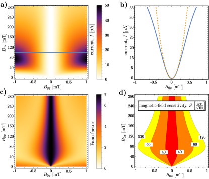
Figure 3: (Color online) Pauli-blockade magnetometry: Magnetic-field sensitivity of a double quantum dot. Numerically calculated (a) current, (c) Fano factor, and (d) magnetic-field sensitivity. The suppressed current around $B_{0z}=0$ in (a) is due to $T_{0}$ blockade. (b) Blue line shows the horizontal cut along the blue line ($B_{0x}=100\ \text{mT}$) in (a). Dashed orange line shows the corresponding perturbative result Eq. (5). The optimal value of the sensitivity in (d) is $S_{\text{opt}}=37\ \text{nT}/\sqrt{\text{Hz}}$, at the point $(B_{0z},B_{0x})=(0,25)\ \text{mT}$. Parameters: $g_{\parallel}=30$, $g_{\perp}=1$, $\Gamma_{R}=\Gamma_{L}=1$ GHz, $t=5\;\mu$eV, $\Delta=0\,\mu\text{eV}$, $\alpha=3^{\circ}$.

To explore the achievable magnetic-field sensitivity of the device in a broader magnetic-field range, and to corroborate our perturbative results discussed so far, we numerically calculated the current, the Fano factor, and the sensitivity. The dependence of these quantities on the offset magnetic field are shown in Fig. 3a,c and d, respectively, for the parameter values given in the figure caption. In Fig. 3b, the blue solid line shows the current along the horizontal cut in Fig. 3a, whereas the orange dashed line shows the corresponding perturbative result Eq. (5). The numerical results in Fig. 3 do confirm our analytical results obtained for the vicinity of the $T_{0}$ blockade, $B_{0z}\approx 0$: On the one hand, the two curves coincide in that region in Fig. 3b; on the other hand, the maximum of the Fano factor in Fig. 3c is indeed $F=7$ as predicted by Eq. (6).

The key features of the results in Fig. 3 are the following. (i) Figure 3a shows that the current is blocked at $B_{0z}=0$; that is the $T_{0}$ blockade. In its vicinity, the current shows a quadratic dependence of $B_{0z}$, as testified by the line cut in Fig. 3b and our perturbative result Eq. (5), and essentially no dependence on $B_{0x}$. This implies that indeed, the device as a magnetometer is directionally sensitive, that is, variations of the current are caused by variations of the $z$ component of the external magnetic field only. (ii) Fig. 3d shows that the best sensitivities are achieved in the vicinity of the central vertical region (black), which indeed roughly coincides with the $T_{0}$ blockade region, i.e., the white vertical region with suppressed current in Fig. 3a and the dark $F\approx 7$ vertical region in the Fano factor plot Fig. 3c. (iii) The current in Fig. 3 shows maxima around $(B_{0z},B_{0x})=(\pm 1\,\text{mT},80\,\text{mT})$. The reason for this is that singlet-triplet mixing is most efficient in these magnetic-field ranges. At these dark spots, the local effective magnetic fields $\hat{g}_{L}\text{\boldmath{$B$}}$ and $\hat{g}_{R}\text{\boldmath{$B$}}$ in the two dots differ significantly, and their energy scales $|\mu_{B}\hat{g}_{L}\text{\boldmath{$B$}}|$ and $|\mu_{B}\hat{g}_{R}\text{\boldmath{$B$}}|$ are comparable to the interdot tunnel amplitude $t$; these conditions ensure efficient singlet-triplet mixingJouravlev and Nazarov (2006) and a large current as seen in Fig. 3a. If the magnetic field is oriented along the same direction, but decreased in magnitude, $|\mu_{B}\hat{g}_{L,R}\text{\boldmath{$B$}}|\ll t$, then the hybridized singlet states with energies around $\pm\sqrt{2}t$ are hardly mixed with the triplets around zero energy, hence the latter ones block transport and the current decreases, as seen in Fig. 3a.

To conclude, we characterized the ultimate sensitivity of a directionally sensitive magnetometry scheme, where the sharp, magnetic-field-induced variations of the current through a Pauli-blockaded DQD are used to measure small changes of the external magnetic field. Using parameter values taken from CNT DQD experiments, we estimate that the sensitivity of such a device can reach a few tens of $\text{nT}/\sqrt{\text{Hz}}$.

V Discussion

V.1 The role of the temperature

Based on Eq. (2), we argued that the optimal sensitivity of the Coulomb-blockade magnetometer is degraded if the temperature is increased. On the other hand, the sensitivity of a Pauli-blockade magnetometer is not influenced directly by the temperature, see Eq. (7). The only requirement on temperature for the Pauli-blockade magnetometry scheme to work is that the orbital level spacing of the dots should dominate the thermal energy scale. One remarkable consequence of this fact is that downsizing the proposed Pauli-blockade magnetometry scheme, e.g., using an atom-sized DQD based on small donor ensemblesWeber et al. (2012, 2014), which would provide larger orbital level spacings, should allow for a higher temperature of operation. Such a miniaturization would provide an added benefit: enhanced spatial resolution.

V.2 Optimal sensitivity and dynamical range for the Pauli-blockade magnetometer

The optimal value of the sensitivity in Fig. 3d is $S_{\text{opt}}=37\ \text{nT}/\sqrt{\text{Hz}}$, at the point $(B_{0z},B_{0x})=(0,25)\ \text{mT}$. However, this is not a suitable working point if we want to use the device as a linear detector of $\delta B_{z}$, since the dependence of the current on $\delta B_{z}$ is quadratic here, see Eq. 5 and Fig. 3b. In other words, even though the sensitivity is optimal at this working point, the dynamical range of the device as a linear detector of $\delta B_{z}$ is zero. Therefore, in practice, the achievable optimal sensitivity is slightly degraded with respect to $S_{\text{opt}}$, and depends on the desired dynamical range. For example, according to Figs. 3b,d, choosing the working point around $(B_{0z},B_{0x})=(0.25,100)\,\text{mT}$, results in a dynamical range of a few hundred microteslas and a sensitivity around $50\,\text{nT}/\sqrt{\text{Hz}}$.

V.3 The role of electric potential fluctuations

Electric potential fluctuations might arise from, e.g., gate voltage noise or the randomly varying occupation of charge traps near the dots. These fluctuations modify the parameters of the quantum dot system; for example, they detune the dots’ energy levels from their pre-defined positions. This could degrade the sensitivity of the Coulomb-blockade magnetometry scheme presented in Sec. III, since the noise-induced random detuning of the energy levels competes with the magnetic energy shift which one wants to measure.

The detailed quantitative characterization of the role of electric potential fluctuations is postponed for future work. We note, however, that these fluctuations are qualitatively different from the shot noise treated in this work, in the sense that shot noise imposes an unavoidable, fundamental limitation on the magnetometer’s sensitivity, whereas the role and importance of the electric potential fluctuations is device dependent, and can probably be mitigated by technological advancements resulting in noise suppression. Also, we emphasize that Coulomb-blockade electrometry, using similar setups as proposed here, has been successfully realizedYoo et al. (1997); Honig et al. (2013) in spite of the electric potential fluctuations present in real devices; this fact further supports the feasibility of Coulomb-blockade magnetometry.

Furthermore, our perturbative result (4) suggests that Pauli-blockade magnetometry enjoys some protection against electrical potential fluctuations: the overlap (4) and hence the decay rate $\bar{\Gamma}=2\Gamma_{R}\left|\langle S_{g}|\bar{T}_{0}\rangle\right|^{2}$ of $\bar{T}_{0}$ are independent of the (1,1)-(0,2) energy detuning $\Delta$. Therefore, even if a weak noise induces fluctuations of $\Delta$, the decay rate $\bar{\Gamma}$ and hence the characteristics of current flow through the device remain unchanged, and the sensitivity of the magnetometer will not be degraded. We also note that the alternative Coulomb-blockade magnetometry scheme, corresponding to the vicinity of the working point $\square$ in Fig. 2d, also enjoys protection against electrical potential fluctuations; see Appendix B for a discussion.

V.4 Different g factors in the two dots

In section IV, we considered a model of a DQD where the principal values $g_{\parallel}$ and $g_{\perp}$ of the $g$-tensors are identical in the two dots. Within this model, the two key qualitative results we have emphasized were the following. (i) If the homogeneous magnetic field $\text{\boldmath{$B$}}_{0}$ is oriented along $x$, then the $T_{0}$ blockade sets in, and the dependence of the current on the component of the magnetic field that is in the $xz$ plane and perpendicular to $\text{\boldmath{$B$}}_{0}$ allows the measurement of the latter. (ii) The independence of the decay rate $\bar{\Gamma}$ from the detuning $\Delta$ indicates that the magnetic-field sensitivity of the Pauli-blockade magnetometry is robust against electric potential fluctuations. We emphasize that these two results are not restricted to the case when $g_{\perp}$ and $g_{\parallel}$ are identical in the two dots; if the g tensors are more generic, but still allow for the $T_{0}$ blockade to appear, then both properties (i) and (ii) remain. The generic condition for the $T_{0}$ blockade is that the local effective magnetic fields on the two dots should have the same absolute values:Jouravlev and Nazarov (2006) $|{\bf{\hat{g}}}_{L}\text{\boldmath{$B$}}|=|{\bf{\hat{g}}}_{R}\text{\boldmath{$B$}}|$. If such a magnetic-field orientation exists for the given g-tensors, and the field is oriented along that direction, then a a single (1,1) two-electron triplet state is decoupled from the others and blocks the current. If we take the spin quantization axis along ${\bf{\hat{g}}}_{L}\text{\boldmath{$B$}}+{\bf{\hat{g}}}_{L}\text{\boldmath{$B$}}$, then this blocking state is in fact $T_{0}=\frac{1}{\sqrt{2}}(\uparrow\downarrow+\downarrow\uparrow)$.

V.5 Mechanical stability requirement for the Pauli-blockade magnetometer

If the particular realization of the Pauli-blockade magnetometry discussed here is used as a scanning probe, then an important requirement is the mechanical stability of the setup. This requirement is related to the fact that in the Pauli-blockade magnetometry setup, the measured quantity (current) is sensitive to a magnetic-field component that is perpendicular to the offset field. Recall that in the Pauli-blockade magnetometry, a homogeneous external magnetic field (offset field) is applied, which is almost aligned with the x axis of the reference frame; for example, $\text{\boldmath{$B$}}_{0}=(100,0,0.25)$ mT. Then, measuring the current provides a measurement of $\delta B_{z}$, that is, the z component of the unknown part of the magnetic field. However, in the presence of weak mechanical noise, influencing either the offset field direction or the DQD orientation, their enclosed angle will change. For example, consider the change when, due to some mechanical instability, the offset field suffers an unwanted rotation $\text{\boldmath{$B$}}_{0}\mapsto\text{\boldmath{$B$}}^{\prime}_{0}$ around the y axis with a small angle $\beta=1/50\approx 1$ degree. This change will give rise to an offset-field z component $B^{\prime}_{0z}\approx B_{0x}\sin\beta\approx 2$ mT, far exceeding the original working-point value $B_{0z}=0.25$ mT. This observation highlights the requirement of a high degree of mechanical stability in potential future devices realizing the proposed magnetometry scheme.

V.6 Realization

The key elements of the schemes studied here have already been realized in CNT-based quantum dot systems, suggesting the feasibility of the outlined principles. Note that the spin degree of freedom in the models used in this work correspond to the combined spin-valley states in CNTs that form twofold degenerate Kramers doublets in the absence of a magnetic fieldLaird et al. (2015).

High-quality single and double dotsLaird et al. (2015); Minot et al. (2004); Kuemmeth et al. (2008); Churchill et al. (2009a, b); Steele et al. (2009); Jespersen et al. (2011); Waissman et al. (2013); Benyamini et al. (2014), including those in bent CNTsLai et al. (2014); Pei et al. (2012); Laird et al. (2013); Hels et al. (2016), have been fabricated. Longitudinal g-factors up to $g_{\parallel}\approx 50$ have been measuredKuemmeth et al. (2008), and Pauli blockade was observedChurchill et al. (2009a, b); Pei et al. (2012); Laird et al. (2013). Part of the experimental data in a bent-CNT DQD (see Fig. S7 in the Supplementary Information of Ref. Pei et al., 2012) and its comparison with theory (see Fig. 1c in Ref. Széchenyi and Pályi, 2015) suggest that in that device, the $g$-tensors show the characteristics required to realize the scheme proposed here, and that the $T_{0}$ blockade (referred to as ‘antiresonance’ in Ref. Széchenyi and Pályi, 2015) have already been observed.

Scanning-probe devices based on quantum dotsYoo et al. (1997), including a gate-tunable CNT quantum dotHonig et al. (2013), have already been fabricated and used for imaging electric fields. Besides demonstrating that CNT dots are compatible with scanning-probe technology, the latter fact also highlights the opportunity to use quantum dots as hybrid sensors, with in situ switching capability between electric-field and magnetic-field sensing.

Nuclear spins can provide a strong magnetic noise for the electron spins via the hyperfine interactionHanson et al. (2007), and therefore their presence is expected to degrade the performance of the magnetometer setups described in this work. This effect might be detrimental for magnetic-field sensing with dots in frequenty used III-V semiconductor hosts, such as GaAs, InAs or InSb, where the strength of the hyperfine-induced magnetic noise is in the millitesla rangeKoppens et al. (2005). It is natural to expect that this noise strength also sets the lower limit of the magnetic-field resolution of the magnetometry schemes described here. One strategy to overcome this limitation is to use dynamical techniques to control the nuclear-spin ensemble Reilly et al. (2008); Shulman et al. (2014), and thereby reduce the randomness of the corresponding effective magnetic field acting on the electrons. Another strategy is to use a host material with a low abundance of nuclear spins. For example, natural CNTs offer a low, 1% abundance of nuclear spins, which can be further lowered using isotopic purification, mitigating the harmful effect of the nuclear-spin bath. We also note that isotopic purification of carbon (diamond) and silicon has already been provenItoh and Watanabe (2014) to be a successful way to substantially reduce hyperfine-induced magnetic noise and thereby effectively prolong electron-spin coherence times in these materials.

VI Conclusions

We have presented two magnetic-field sensing principles, which are based on electron transport in Coulomb- and Pauli-blockaded quantum dots. We demonstrated that the fundamental limit of the magnetic-field sensitivity in such devices can be below $\mu\textrm{T}/\sqrt{\textrm{Hz}}$. A carbon nanotube might be optimal as a host material. Downsizing the proposed scheme, e.g., using an atomic-sized double quantum dot based on small donor ensembles, might lead to further improved spatial resolution, and, as a consequence of higher orbital level spacings, a broader temperature range of operation.

Appendix A Derivation of the sensitivity formula

Here we show that the shot-noise-limited magnetic-field sensitivity of a current-based magnetometer is characterized by Eq. (1). The notation used here follows that introduced in the main text.

Charge flow through the device has a random character, since electron tunneling between the leads and the conductor occur in a random fashion. To describe this randomness, we use $P(N,\tau)$, the probability that in the time window between $t=0$ and $t=\tau$, the number of electrons entering the drain contact is $N$. The normalization condition is that $\sum_{N\in\mathbb{Z}}P(N,\tau)=1$ for any $\tau$. Henceforth we assume that the device is in its steady state, and that $P(N,\tau)$ corresponds to this steady state.

We assume that the current is measured by counting the electrons entering the drain during the measurement time window $t\in[0,\tau]$. The number of transmitted electrons is a random variable; let us characterize its probability distribution by its average $\mathcal{N}(\tau)=\sum_{N\in\mathbb{Z}}NP(N,\tau)$ and its variance $\sigma^{2}(\tau)=\sum_{N\in\mathbb{Z}}\left[N-\mathcal{N}(\tau)\right]^{2}P(N,\tau)$. Note that in the steady state, both quantities are proportional to the measurement time $\tau$ (see Refs. Bagrets and Nazarov, 2003; Belzig, 2005 and Eqs. (15) and (16) below), which motivates the definitions of the electric current $I$ and the Fano factor $F$,

$$I = -e\mathcal{N}(\tau)/\tau,$$ (8)

$$F = \sigma^{2}(\tau)/\mathcal{N}(\tau),$$ (9)

which are $\tau$-independent quantities. Here, $e$ denotes the absolute value of the electron charge.

In the considered generic magnetometer, both the average and the variance depend on the magnetic field, $\mathcal{N}(\tau)=\mathcal{N}(\tau,B)$ and $\sigma^{2}(\tau)=\sigma^{2}(\tau,B)$. The task is the following. Assume that $I(B)$ is known, and that a known working-point magnetic field $B_{0}$ is switched on. There is also an unknown small component $\delta B$ of the magnetic field $B=B_{0}+\delta B$. We wish to determine $\delta B$ by measuring the number of electrons entering the drain contact in a given measurement time window $\tau$. That is possible, if the change of the average number of transmitted electrons induced by $\delta B$ exceeds the standard deviation of the transmitted electrons at the working point. This condition is formalized as

$$|\mathcal{N}(\tau,B_{0}+\delta B)-\mathcal{N}(\tau,B_{0})|>\sigma(\tau,B_{0}).$$ (10)

This condition leads to a natural definition of the magnetic-field sensitivity in accordance with Eq. (1): After (i) linearizing Eq. (10) in $\delta B$, (ii) expressing the resulting formula in terms of the current $I$ and Fano factor $F$ defined in Eqs. (8) and (9), and (iii) rearranging the two sides of the resulting equation, we find that the minimal change in magnetic field that can be resolved by the current measurement is constrained by

$$|\delta B|>\frac{1}{\sqrt{\tau}}\frac{\sqrt{eF(B_{0})I(B_{0})}}{|I^{\prime}(B_{0})|}$$ (11)

where the prime denotes the derivative with respect to the magnetic field.

We conclude that the second fraction on the right hand side of Eq. (11), defined as the magnetic-field sensitivity $S$ in Eq. (1), does indeed characterize the performance of the magnetometer: for a given measurement time $\tau$, the minimum resolvable change in the magnetic field is $S/\sqrt{\tau}$.

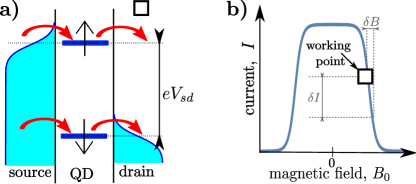
Figure 4: Alternative operation of a Coulomb-blockade magnetometer. (a) Level diagram corresponding to the optimal-sensitivity working point marked by $\square$ in Fig. 2c. Here, the offset magnetic field and the source-drain bias are chosen so that the two spin levels are aligned with the chemical potentials of the two leads. (b) Magnetic-field dependence of the current in the vicinity of the working point $\square$. The width of the current plateau is $\sim eV_{sd}/g\mu_{B}$, that is, it is set by the source-drain bias $V_{sd}$. The width of the slopes connecting the zero-current range with the current plateau is $\sim k_{B}T/g\mu_{B}$, that is, it is set by the temperature $T$.

Appendix B An alternative scheme of Coulomb-blockade magnetometry

In Fig. 2d, the global minimum of the magnetic-field sensitivity $S$ is at the point marked by the white square $\square$, that is, at $(\epsilon,B_{0})\approx(0\,\mu\text{eV},10\,\text{mT})$. As mentioned in section III, the operation of the magnetometer at this working point does not follow the scheme proposed there: the level alignment is not as shown in Fig. 1b. We show the schematic level alignment for the working point $\square$ in Fig. 4a: each Zeeman-split level is located in the vicinity of the chemical potential of one of the leads. In this situation, the dependence of the current on the magnetic field is due to the following reason. A small change $\delta B>0$ in the magnetic field shifts the energy of the $\downarrow$ ($\uparrow$) state downwards (upwards), therefore the outgoing (incoming) rate towards the drain (from the source) decreases. That is, transport through both levels is suppressed, and therefore the current decreases, as shown schematically in Fig. 4b.

We expect that the effect of electrical potential fluctuations, that is, the effect of the noise of the on-site energy $\epsilon$, can be mitigated by choosing a special working point in the vicinity of $\square$. We illustrate this opportunity using Fig. 5. Figure 5a shows the current as a function of the magnetic field $B_{0}$ and the on-site energy $\epsilon$, whereas Fig. 5b shows the derivative of the current with respect to the on-site energy, $\frac{\partial I}{\partial\epsilon}$. A strongly reduced effect of $\epsilon$-noise on the magnetic-field sensitivity is expected in the working points along the contour where $\frac{\partial I}{\partial\epsilon}=0$ (see Fig. 5b). In order to simultaneously exploit the opportunity for charge-noise resilience and obtain a good magnetic-field sensitivity $S$, one should find the minimum of $S$ along the $\frac{\partial I}{\partial\epsilon}=0$ contour. The resulting optimal working point is denoted with the black star in Fig. 5c, where the sensitivity is shown together with the $\frac{\partial I}{\partial\epsilon}=0$ contour (solid blue line). The sensitivity corresponding to this optimal working point is $S_{\text{opt}}\approx 2\,\mu\text{T}/\sqrt{\text{Hz}}$.

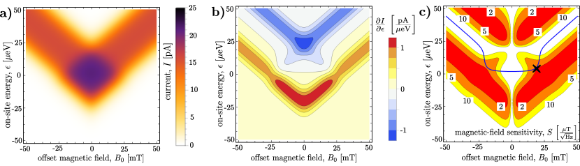
Figure 5: Charge-noise-resilient working point of the Coulomb-blockade magnetometer. (a) Current $I(B_{0},\epsilon)$ as a function of the magnetic field and the quantum dot on-site energy. (b) Derivative of the current with respect to the on-site energy. Working points along the contour $\frac{\partial I}{\partial\epsilon}=0$ are expected to have a reduced susceptibility to charge noise (i.e., fluctuations of $\epsilon$). (c) Magnetic-field sensitivity $S(B_{0},\epsilon)$. The solid blue line is the $\frac{\partial I}{\partial\epsilon}=0$ contour. The black star is the working point where the magnetic-field sensitivity is optimized ($S_{\text{opt}}\approx 2\,\mu\text{T}/\sqrt{\text{Hz}}$) along the contour. Parameters: same as in Fig. 2, except that $V_{sd}=43\,\mu\text{V}$.

Appendix C Calculating current and shot noise using rate equations

Here, we present the counting-field methodBagrets and Nazarov (2003); Belzig (2005) we used to calculate the current and the shot noise of the considered setups, and outline the derivation of the specific results for the Coulomb-blockade and Pauli-blockade magnetometers.

C.1 Generic framework to calculate the current and the shot noise: the counting-field method

The transport process consists of single-electron tunneling events between the source and the conductor and between the conductor and the drain. Electrons in the conductor can occupy $M$ different states; for example, in the Coulomb-blockade magnetometer setup we consider in section III we have $M=3$, as there are three electronic states involved in the transport cycle: the empty dot, and the two Zeeman-split single-electron states $\downarrow$ and $\uparrow$. We assume that the number of charges arriving to the drain is being measured from some initial point $t=0$ in time. Then, the random character of the tunneling events is described by the probability density function $P_{i}(N,\tau)$ where $i=1,\dots,M$; $N\in\mathbb{Z}$; $\tau>0$: this is the probability of that at time $\tau$, the conductor is in its $i$the electronic state, and $N$ electrons have arrived to the drain since $t=0$. Note that the relation between the probability $P_{j}(N,\tau)$ introduced here and the probability $P(N,\tau)$ introduced in section A is simply $P(N,\tau)=\sum_{i=1}^{M}P_{i}(N,\tau)$. The normalization condition reads $\sum_{i=1}^{M}\sum_{N\in\mathbb{Z}}P_{i}(N,\tau)=1$ for all $\tau$. We introduce the vector $\mathbf{P}(N,\tau)=\left(P_{1}(N,\tau),\dots,P_{M}(N,\tau)\right)$. The time evolution of $\mathbf{P}(N,\tau)$ is governed by a rate equation and depends on the initial (in general, mixed) electronic state characterized by $\mathbf{P}(0,0)$. However, here we focus only on the steady-state current and shot noise, and disregard transient effects.

The effect of random single-electron tunneling events is described by the following rate equation:

$$\partial_{\tau}\mathbf{P}(N,\tau)=\boldsymbol{\Gamma}_{0}\mathbf{P}(N,\tau)+\boldsymbol{J}^{+}\mathbf{P}(N-1,\tau)+\boldsymbol{J}^{-}\mathbf{P}(N+1,\tau),$$ (12)

where the rate matrices $\boldsymbol{\Gamma}_{0}$, $\boldsymbol{J}^{+}$ and $\boldsymbol{J}^{-}$ have size $M\times M$. The matrix $\boldsymbol{J}^{+}$ ($\boldsymbol{J}^{-}$) represents single-electron tunneling events from the conductor to the drain (from the drain to the conductor). For a concrete example for such a rate equation, see Eq. (C.2), the one for the Coulomb-blockade magnetometer.

As the rate matrices are independent of $N$, the infinite coupled set (12) of differential equations can be partially decoupled with the following Fourier transformation:

$$\tilde{\mathbf{P}}(\chi,\tau)=\sum_{N\in\mathbb{Z}}\mathbf{P}(N,\tau)\;e^{iN\chi},$$ (13)

where $\chi\in]-\pi,\pi]$. Acting on Eq. (12) with this Fourier transformation yields

$$\partial_{\tau}\tilde{\mathbf{P}}(\chi,\tau)=(\boldsymbol{\Gamma}_{0}+\boldsymbol{J}^{+}e^{i\chi}+\boldsymbol{J}^{-}e^{-i\chi})\tilde{\mathbf{P}}(\chi,\tau)=\boldsymbol{M}(\chi)\tilde{\mathbf{P}}(\chi,\tau).$$ (14)

Here the second equality is the definition of $\boldsymbol{M}(\chi)$, and $\chi$ is referred to as the counting field. For every value of $\chi$, Eq. (14) represents a coupled set of $M$ differential equations.

As shown in Refs. Bagrets and Nazarov, 2003; Belzig, 2005, the steady-state current and the steady-state shot noise are both related to the eigenvalue branch $\lambda_{1}(\chi)$ of $\boldsymbol{M}(\chi)$ that fulfills $\lambda_{1}(\chi=0)=0$. The average number of transmitted electrons in the steady state is

$$\mathcal{N}(\tau)=\sum_{N\in\mathbb{Z}}NP(N,\tau)=-i\left.\tau\frac{\partial\lambda_{1}(\chi)}{\partial\chi}\right|_{\chi=0},$$ (15)

whereas the variance is

$$\sigma^{2}(\tau)=\sum_{N\in\mathbb{Z}}\left[N^{2}-\mathcal{N}^{2}(\tau)\right]P(N,\tau)=-\left.\tau\frac{\partial^{2}\lambda_{1}(\chi)}{\partial\chi^{2}}\right|_{\chi=0}.$$ (16)

These equations are then used to express the current via Eq. (8) and the Fano factor via Eq. (9). To obtain the numerical results shown in Figs. 2 and 3, we have numerically evaluated the first and second derivatives of $\lambda_{1}(\chi)$ after numerical diagonalization of the matrix $\boldsymbol{M}(\chi)$ at $\chi=0$ and $\chi=\pm 10^{-5}$.

C.2 Rate equation for the Coulomb-blockade magnetometer

The rate equation describing electron transport through the Coulomb-blockade magnetometer, i.e., a single quantum dot, reads:

$$\dot{P}_{\sigma}(N,\tau) = -\sum_{s}\Gamma_{\sigma,s}^{\textrm{out}}P_{\sigma}(N,\tau)+\Gamma_{\sigma,L}^{\textrm{in}}P_{0}(N,\tau)+$$

$$+ \Gamma_{\sigma,R}^{\textrm{in}}P_{0}(N+1,\tau),$$

$$\dot{P}_{0}(N,\tau) = \sum_{\sigma}\Gamma_{\sigma,R}^{\textrm{out}}P_{\sigma}(N-1,\tau)+\sum_{\sigma}\Gamma_{\sigma,L}^{\textrm{out}}P_{\sigma}(N,\tau)-$$ (17)

$$- \sum_{\sigma,s}\Gamma_{\sigma,s}^{\textrm{in}}P_{0}(N,\tau),$$

where $\sigma\in\{\downarrow=-1,\uparrow=+1\}$ and the indices of the leads are $s\in\{L,R\}$. Here, $P_{0}(N,\tau)$ is the joint probability of the event that the dot is empty at time $\tau$ and $N$ electrons have entered the drain between $t=0$ and $t=\tau$. Similarly, $P_{\uparrow}(N,\tau)$ $\left[P_{\downarrow}(N,\tau)\right]$ is the joint probability of the event that the dot is occupied with a spin-up [spin-down] electron at time $\tau$, and $N$ electrons have entered the drain between $t=0$ and $t=\tau$. Furthermore, the transition rates $\Gamma_{\sigma,s}^{\textrm{in}}=\Gamma f_{\textrm{FD}}(\epsilon_{\sigma}-\mu_{s})$ and $\Gamma_{\sigma,s}^{\textrm{out}}=\Gamma\left(1-f_{\textrm{FD}}(\epsilon_{\sigma}-\mu_{s})\right)$ are expressed using the lead-dot tunnelling rate $\Gamma$ and the Fermi-Dirac distribution $f_{\textrm{FD}}(x)=\frac{1}{e^{x/(k_{B}T)}+1}$. The chemical potentials are biased symmetrically $\mu_{L}=-\mu_{R}=\frac{eV_{sd}}{2}$. Due to the Zeeman splitting, the spin-dependent energy of the single occupied dot is $\epsilon_{\sigma}=\epsilon+\frac{1}{2}\sigma g\mu_{B}B$.

Using this rate equation, we apply the counting-field method outlined above to calculate the current and the Fano factor. We used analytical results for the current to generate Figs. 2a,b and 5a, 5b. The Fano factor shown in 2c, as well as the sensitivities shown in Figs. 2d and 5c, are evaluated numerically.

C.3 Rate equation for the Pauli-blockade magnetometer

Here, we present the rate equation we use to describe the transport process through the considered Pauli-blockaded double quantum dot. The rates of $(0,1)\rightarrow(1,1)$ [$(0,2)\rightarrow(0,1)$] transitions are parametrized by the rate $\Gamma_{L}$ [$\Gamma_{R}$], describing single-electron tunneling from the source to the left dot [from the right dot to the drain]. These considerations result in the following classical master equation Széchenyi and Pályi (2013):

$$\dot{P}_{j}(N,\tau) = -2\Gamma_{R}v_{j}P_{j}(N,\tau)+\frac{1}{2}\Gamma_{\rm L}(1-v_{j})P_{6}(N,\tau),$$

$$\dot{P}_{6}(N,\tau) = -2\Gamma_{\rm L}P_{6}(N,\tau)+2\Gamma_{R}\sum_{j=1}^{5}v_{j}P_{j}(N-1,\tau).$$ (18)

Here, $P_{j}(N,\tau)$ with $j\in\{1,2,3,4,5\}$ is the joint probability of the event that the $j$-th two-electron energy eigenstate $\Psi_{j}$ of the double-dot Hamiltonian $H=H_{B}+H_{\textrm{tun}}+H_{\Delta}$ (see main text) is occupied at time $\tau$ and $N$ electrons have entered the drain between $t=0$ and $t=\tau$. Similarly, $P_{6}(N,\tau)$ is the joint probability of the event that a (0,1) state is occupied, and $N$ electrons have entered the drain between $t=0$ and $t=\tau$. Furthermore, $v_{j}$ [$1-v_{j}$] is the weight of the two-electron energy eigenstate $\Psi_{j}$ in the (0,2) [(1,1)] charge configuration, that is, $v_{j}=\left|\langle\Psi_{j}|S_{g}\rangle\right|^{2}$; note that $\sum_{j=1}^{5}v_{j}=1$.

C.4 Perturbative analytical results for the current and the shot noise in the vicinity of $T_{0}$ blockade

In the description of the Pauli-blockade magnetometer in section IV, we quote analytical results for the electrical current, Eq. 5, and the Fano factor, Eq. 6. These results are valid in the case when $B_{z}$ is sufficiently small, that is, when the decay rate $\bar{\Gamma}$ of the state $\bar{T}_{0}$ is much smaller than any other transition rate in the rate equation (C.3). To arrive to these analytical results, we use the perturbative technique applied in Ref. Belzig, 2005. The key steps are: (i) The size of $\boldsymbol{M}(\chi)$ is $6\times 6$, hence the characteristic polynomial of $\boldsymbol{M}(\chi)$ is of sixth order, $C(\lambda,\bar{\Gamma})=\sum_{i=1}^{6}c_{i}(\bar{\Gamma})\lambda^{i}$; here the coefficients $c_{i}(\bar{\Gamma})$ are explicitly determined by the matrix elements of $\boldsymbol{M}(\chi)$. (ii) For $\bar{\Gamma}=0$, the state $T_{0}$ is the steady state, with the corresponding eigenvalue $\lambda_{1}(\bar{\Gamma}=0)=0$. (iii) For small but nonzero $\bar{\Gamma}$, the eigenvalue $\lambda_{1}$ developing from $\lambda_{1}(\bar{\Gamma}=0)=0$ is assumed to be linear in $\bar{\Gamma}$, that is, of the form $\lambda_{1}=\alpha\bar{\Gamma}$. (iv) Substituting $\lambda=\alpha\bar{\Gamma}$ to the characteristic polynomial $C(\lambda,\bar{\Gamma})$, first-order Taylor-expanding the latter in $\bar{\Gamma}$, and equating the result to zero, yields the linear equation

$$C(\lambda,\bar{\Gamma})\approx\left.\frac{dc_{0}(\bar{\Gamma})}{d\bar{\Gamma}}\right|_{\bar{\Gamma}=0}\bar{\Gamma}+c_{1}(0)\alpha\bar{\Gamma}=0.$$ (19)

Solving this for $\alpha$ yields

$$\lambda_{1}(\chi)=\alpha\bar{\Gamma}=-\frac{\left.\frac{dc_{0}(\bar{\Gamma})}{d\bar{\Gamma}}\right|_{\bar{\Gamma}=0}}{c_{1}(0)}\bar{\Gamma}=-4\bar{\Gamma}\frac{1-e^{i\chi}}{4-3e^{i\chi}}.$$ (20)

This result was used, together with Eqs. (15) and (16) to obtain the results for the current and the Fano factor.

Appendix D Resilience to charge noise: detuning-independent decay rate of $\bar{T}_{0}$

Here we provide the derivation of Eq. (4) of the main text. As stated there, we use first-order perturbation theory to arrive to the result. Nevertheless, we do present the derivation here as it involves one nontrivial technical step: Usually, the application of perturbation theory is based on the knowledge of the eigensystem of the unperturbed Hamiltonian; we do not have that knowledge here, which necessitates an alternative approach to arrive to the result.

We start by evaluating the two-electron Hamiltonian $H=H_{B}+H_{\textrm{tun}}+H_{\Delta}$ (see main text) exactly at the $T_{0}$ blockade, that is, at $\text{\boldmath{$B$}}=(B,0,0)$. We set the spin quantization axis along $x$, and express $H$ in the basis $T_{+}$, $T_{-}$, $S$, $S_{g}$, $T_{0}$; the corresponding matrix reads Jouravlev and Nazarov (2006); Danon et al. (2013); Széchenyi and Pályi (2015)

$$H_{0}=\left(\begin{array}[]{cccc | c}\mathcal{B}_{s}&0&-\mathcal{B}_{a\perp}/\sqrt{2}&0&0\\ 0&-\mathcal{B}_{s}&\mathcal{B}_{a\perp}/\sqrt{2}&0&0\\ -\mathcal{B}_{a\perp}/\sqrt{2}&\mathcal{B}_{a\perp}/\sqrt{2}&0&\sqrt{2}t&0\\ 0&0&\sqrt{2}t&-\Delta&0\\ \hline\cr 0&0&0&0&0\end{array}\right).$$ (26)

where $\mathcal{B}_{s}=\frac{1}{2}\mu_{B}\left[(\hat{\boldsymbol{g}}_{L}+\hat{\boldsymbol{g}}_{R})\text{\boldmath{$B$}}\right]_{x}$ and $\mathcal{B}_{a\perp}=\frac{1}{2}\mu_{B}[(\hat{\boldsymbol{g}}_{L}-\hat{\boldsymbol{g}}_{R})\text{\boldmath{$B$}}]_{z}$. The upper left $4\times 4$ block of $H_{0}$ will be referred to as $H^{\prime}_{0}$. In $H_{0}$, the unpolarized triplet $T_{0}$ is decoupled from the other states and therefore blocks the current. A finite magnetic-field component along $z$, entering the Hamiltonian as a perturbation $H_{1}=\mathcal{B}_{a\parallel}(|T_{0}\rangle\langle S|+h.c.)$, mixes $T_{0}$ with the other states. Here $\mathcal{B}_{a\parallel}=\frac{1}{2}\mu_{B}[(\hat{\boldsymbol{g}}_{L}-\hat{\boldsymbol{g}}_{R})\text{\boldmath{$B$}}]_{x}$, and we will denote the perturbed $T_{0}$ state by $\bar{T}_{0}$.

We were unable to find analytical expressions for the eigensystem of $H^{\prime}_{0}$, which would have provided a convenient starting point for doing perturbation theory in $H_{1}$. However, the overlap $\langle S_{g}|\bar{T}_{0}\rangle$ we are looking for, which determines the decay rate of the blocking state $\bar{T}_{0}$, can be expressed in an alternative way. Start with the standard first-order perturbative formula for the energy eigenstates:

$$\langle S_{g}|\bar{T}_{0}\rangle = \langle S_{g}|\left[|T_{0}\rangle+\sum_{i=1}^{4}\frac{|i\rangle\langle i|H_{1}|T_{0}\rangle}{E(T_{0})-E(i)}\right]$$ (27)

$$= -\mathcal{B}_{a\parallel}\langle S_{g}|(H^{\prime}_{0})^{-1}|S\rangle.$$

Here, $|i\rangle$ and $E(i)$ $(i\in\{1,2,3,4,T_{0}\})$ are the eigenstates and eigenvalues of $H_{0}$, respectively. In the second step, we used the form of $H_{1}$ given above, the value $E(T_{0})=0$, and the fact that $\sum_{i=1}^{4}\frac{|i\rangle\langle i|}{E(i)}=(H^{\prime}_{0})^{-1}$. The $4\times 4$ matrix $H^{\prime}_{0}$ can be inverted analytically, yielding $\langle S_{g}|\bar{T}_{0}\rangle=-\frac{\mathcal{B}_{a\parallel}}{\sqrt{2}t}$. Importantly, this result is independent of the (1,1)-(0,2) energy detuning $\Delta$, which is apparent from the above definition of $\mathcal{B}_{a\parallel}$; this $\Delta$-independence provides the feature of charge-noise-resilience of the proposed magnetometer, discussed in Sec. V.3. Using the conditions $B_{z}\ll B_{x}$, $\alpha\ll 1$, and $g_{\perp}\ll g_{\parallel}$, fulfilled by the realistic parameter set used in the main text, we find $\mathcal{B}_{a\parallel}\approx\mu_{B}B_{z}\alpha\frac{g_{\parallel}^{2}}{g_{\perp}}$, leading to the result (4).

References

- Bending (1999) S. J. Bending, Advances in Physics 48, 449 (1999).
- Martin and Wickramasinghe (1987) Y. Martin and H. K. Wickramasinghe, Applied Physics Letters 50, 1455 (1987).
- Chang et al. (1992) A. M. Chang, H. D. Hallen, L. Harriott, H. F. Hess, H. L. Kao, J. Kwo, R. E. Miller, R. Wolfe, J. van der Ziel, and T. Y. Chang, Applied Physics Letters 61, 1974 (1992).
- Kirtley et al. (1995) J. R. Kirtley, M. B. Ketchen, K. G. Stawiasz, J. Z. Sun, W. J. Gallagher, S. H. Blanton, and S. J. Wind, Applied Physics Letters 66, 1138 (1995).
- Allred et al. (2002) J. C. Allred, R. N. Lyman, T. W. Kornack, and M. V. Romalis, Phys. Rev. Lett. 89, 130801 (2002).
- Rugar et al. (2004) D. Rugar, R. Budakian, H. J. Mamin, and B. W. Chui, Nature 430, 329 (2004).
- Taylor et al. (2008) J. M. Taylor, P. Cappellaro, L. Childress, L. Jiang, D. Budker, P. R. Hemmer, A. Yacoby, R. Walsworth, and M. D. Lukin, Nat Phys 4, 810 (2008).
- Milde et al. (2013) P. Milde, D. Köhler, J. Seidel, L. M. Eng, A. Bauer, A. Chacon, J. Kindervater, S. Mühlbauer, C. Pfleiderer, S. Buhrandt, C. Schütte, and A. Rosch, Science 340, 1076 (2013).
- Switkes et al. (1998) M. Switkes, A. G. Huibers, C. M. Marcus, K. Campman, and A. C. Gossard, Applied Physics Letters 72, 471 (1998).
- Lassagne et al. (2011) B. Lassagne, D. Ugnati, and M. Respaud, Phys. Rev. Lett. 107, 130801 (2011).
- Kirtley et al. (1996) J. R. Kirtley, C. C. Tsuei, M. Rupp, J. Z. Sun, L. S. Yu-Jahnes, A. Gupta, M. B. Ketchen, K. A. Moler, and M. Bhushan, Phys. Rev. Lett. 76, 1336 (1996).
- Pelliccione et al. (2016) M. Pelliccione, A. Jenkins, P. Ovartchaiyapong, C. Reetz, E. Emmanouilidou, N. Ni, and A. C. Bleszynski Jayich, Nat Nano 11, 700 (2016).
- Thiel et al. (2016) L. Thiel, D. Rohner, M. Ganzhorn, P. Appel, E. Neu, B. Müller, R. Kleiner, D. Koelle, and P. Maletinsky, Nat Nano 11, 677 (2016).
- Kezsmarki et al. (2015) I. Kezsmarki, S. Bordacs, P. Milde, E. Neuber, L. M. Eng, J. S. White, H. M. Ronnow, C. D. Dewhurst, M. Mochizuki, K. Yanai, H. Nakamura, D. Ehlers, V. Tsurkan, and A. Loidl, Nat Mater 14, 1116 (2015).
- Wang et al. (2015) X. R. Wang, C. J. Li, W. M. Lü, T. R. Paudel, D. P. Leusink, M. Hoek, N. Poccia, A. Vailionis, T. Venkatesan, J. M. D. Coey, E. Y. Tsymbal, Ariando, and H. Hilgenkamp, Science 349, 716 (2015).
- Bluhm et al. (2009) H. Bluhm, N. C. Koshnick, J. A. Bert, M. E. Huber, and K. A. Moler, Phys. Rev. Lett. 102, 136802 (2009).
- Kalisky et al. (2013) B. Kalisky, E. M. Spanton, H. Noad, J. R. Kirtley, K. C. Nowack, C. Bell, H. K. Sato, M. Hosoda, Y. Xie, Y. Hikita, C. Woltmann, G. Pfanzelt, R. Jany, C. Richter, H. Y. Hwang, J. Mannhart, and K. A. Moler, Nat. Mater. 12, 1091 (2013).
- Spanton et al. (2014) E. M. Spanton, K. C. Nowack, L. Du, G. Sullivan, R.-R. Du, and K. A. Moler, Phys. Rev. Lett. 113, 026804 (2014).
- Nowack et al. (2013) K. C. Nowack, E. M. Spanton, M. Baenninger, M. König, J. R. Kirtley, B. Kalisky, C. Ames, P. Leubner, C. Brüne, H. Buhmann, L. W. Molenkamp, D. Goldhaber-Gordon, and K. A. Moler, Nat Mater 12, 787 (2013).
- Ono et al. (2002) K. Ono, D. G. Austing, Y. Tokura, and S. Tarucha, Science 297, 1313 (2002).
- Korotkov et al. (1992) A. N. Korotkov, D. V. Averin, K. K. Likharev, and S. A. Vasenko, in Single-Electron Tunneling and Mesoscopic Devices (Springer-Verlag Berlin Heidelberg 1992, 1992).
- Blanter and Büttiker (2000) Y. Blanter and M. Büttiker, Physics Reports 336, 1 (2000).
- Korotkov (1994) A. N. Korotkov, Phys. Rev. B 49, 10381 (1994).
- Ajiki and Ando (1993) H. Ajiki and T. Ando, Journal of the Physical Society of Japan 62, 1255 (1993).
- Minot et al. (2004) E. D. Minot, Y. Yaish, V. Sazonova, and P. L. McEuen, Nature 428, 536 (2004).
- Kuemmeth et al. (2008) F. Kuemmeth, S. Ilani, D. C. Ralph, and P. L. McEuen, Nature 452, 448 (2008).
- Laird et al. (2015) E. A. Laird, F. Kuemmeth, G. A. Steele, K. Grove-Rasmussen, J. Nygård, K. Flensberg, and L. P. Kouwenhoven, Rev. Mod. Phys. 87, 703 (2015).
- Bagrets and Nazarov (2003) D. A. Bagrets and Y. V. Nazarov, Phys. Rev. B 67, 085316 (2003).
- Belzig (2005) W. Belzig, Phys. Rev. B 71, 161301 (2005).
- Koppens et al. (2005) F. H. L. Koppens, J. A. Folk, J. M. Elzerman, R. Hanson, L. H. W. van Beveren, T. Vink, H. P. Tranitz, W. Wegscheider, L. P. Kouwenhoven, and L. M. K. Vandersypen, Science 309, 1346 (2005).
- Jouravlev and Nazarov (2006) O. N. Jouravlev and Y. V. Nazarov, Phys. Rev. Lett. 96, 176804 (2006).
- Pfund et al. (2007) A. Pfund, I. Shorubalko, K. Ensslin, and R. Leturcq, Phys. Rev. Lett. 99, 036801 (2007).
- Danon and Nazarov (2009) J. Danon and Y. V. Nazarov, Phys. Rev. B 80, 041301 (2009).
- Pei et al. (2012) F. Pei, E. A. Laird, G. A. Steele, and L. P. Kouwenhoven, Nat. Nanotech. 7, 630 (2012).
- Széchenyi and Pályi (2015) G. Széchenyi and A. Pályi, Phys. Rev. B 91, 045431 (2015).
- Laird et al. (2013) E. A. Laird, F. Pei, and L. P. Kouwenhoven, Nat. Nanotech. 8, 565 (2013).
- Weber et al. (2012) B. Weber, S. Mahapatra, T. F. Watson, and M. Y. Simmons, Nano Letters 12, 4001 (2012).
- Weber et al. (2014) B. Weber, Y. H. M. Tan, S. Mahapatra, T. F. Watson, H. Ryu, R. Rahman, L. C. L. Hollenberg, G. Klimeck, and M. Y. Simmons, Nat Nano 9, 430 (2014).
- Yoo et al. (1997) M. J. Yoo, T. A. Fulton, H. F. Hess, R. L. Willett, L. N. Dunkleberger, R. J. Chichester, L. N. Pfeiffer, and K. W. West, Science 276, 579 (1997).
- Honig et al. (2013) M. Honig, J. A. Sulpizio, J. Drori, A. Joshua, E. Zeldov, and S. Ilani, Nat Mater 12, 1112 (2013).
- Churchill et al. (2009a) H. O. H. Churchill, F. Kuemmeth, J. W. Harlow, A. J. Bestwick, E. I. Rashba, K. Flensberg, C. H. Stwertka, T. Taychatanapat, S. K. Watson, and C. M. Marcus, Phys. Rev. Lett. 102, 166802 (2009a).
- Churchill et al. (2009b) H. O. H. Churchill, A. J. Bestwick, J. W. Harlow, F. Kuemmeth, D. Marcos, C. H. Stwertka, S. K. Watson, and C. M. Marcus, Nature Physics 5, 321 (2009b).
- Steele et al. (2009) G. A. Steele, G. Gotz, and L. P. Kouwenhoven, Nat Nano 4, 363 (2009).
- Jespersen et al. (2011) T. S. Jespersen, K. Grove-Rasmussen, J. Paaske, K. Muraki, T. Fujisawa, J. Nygard, and K. Flensberg, Nat. Phys 7, 348 (2011).
- Waissman et al. (2013) J. Waissman, M. Honig, S. Pecker, A. Benyamini, A. Hamo, and S. Ilani, Nat Nano 8, 569 (2013).
- Benyamini et al. (2014) A. Benyamini, A. Hamo, S. V. Kusminskiy, F. von Oppen, and S. Ilani, Nat Phys 10, 151 (2014).
- Lai et al. (2014) R. A. Lai, H. O. H. Churchill, and C. M. Marcus, Phys. Rev. B 89, 121303 (2014).
- Hels et al. (2016) M. C. Hels, B. Braunecker, K. Grove-Rasmussen, and J. Nygård, Phys. Rev. Lett. 117, 276802 (2016).
- Hanson et al. (2007) R. Hanson, L. P. Kouwenhoven, J. R. Petta, S. Tarucha, and L. M. K. Vandersypen, Rev. Mod. Phys. 79, 1217 (2007).
- Reilly et al. (2008) D. J. Reilly, J. M. Taylor, J. R. Petta, C. M. Marcus, M. P. Hanson, and A. C. Gossard, Science 321, 817 (2008).
- Shulman et al. (2014) M. D. Shulman, S. P. Harvey, J. M. Nichol, S. D. Bartlett, A. C. Doherty, V. Umansky, and A. Yacoby, Nature Communications 5, 5156 EP (2014).
- Itoh and Watanabe (2014) K. M. Itoh and H. Watanabe, MRS Communications 4, 143 (2014).
- Széchenyi and Pályi (2013) G. Széchenyi and A. Pályi, Phys. Rev. B 88, 235414 (2013).
- Danon et al. (2013) J. Danon, X. Wang, and A. Manchon, Phys. Rev. Lett. 111, 066802 (2013).