Bank Card Usage Prediction Exploiting Geolocation Information

Abstract

We describe the solution of team ISMLL for the ECML-PKDD 2016 Discovery Challenge on Bank Card Usage for both tasks. Our solution is based on three pillars. Gradient boosted decision trees as a strong regression and classification model, an intensive search for good hyperparameter configurations and strong features that exploit geolocation information. This approach achieved the best performance on the public leaderboard for the first task and a decent fourth position for the second task.

1 Challenge Description

The goal of one of this year’s ECML-PKDD Discovery Challenges was to predict the behaviour of customers of the Hungarian bank otpbank. The challenge was divided into two tasks. The first task was to predict for every bank branch the number of visits for a set of customers, the second task was to predict, whether a customer will apply for a credit card in the next six months. For these tasks, anonymized customer information (e.g. age, location, income, gender) and bank activities (e.g. what has been bought, where and when) were provided. A labeled data set for 2014 was made available which can be used for supervised machine learning to predict the targets for a disjoint set of customers for 2015. The evaluation measure for Task 2 is the area under the ROC curve (AUC), a very common measure for imbalanced classification problems. The evaluation measure for Task 1 is a little bit more exotic. It is the average of cosine@1 and cosine@5 for every customer $c$ where

$$\text{cosine@k}:=\frac{\sum_{i=1}^{k}y_{c,i}\hat{y}_{c,i}}{\sqrt{\sum_{i=1}^{b}y_{c,i}^{2}}\sqrt{\sum_{i=1}^{k}\hat{y}_{c,i}^{2}}}$$ (1)

with $y_{c,i}$ being the number of times the customer $c$ has visited bank branch $i$ and $\hat{y}_{c,i}$ the prediction, respectively. There are $b$ different branches in total. For more information we refer to the challenge website [1].

2 Problem Identification

For the first task, we assumed that there is no relation between the number of visits of a customer among branches. This enabled us to tackle $b$ different regression tasks for each of the $b$ branches. Independently, we trained a regression model for each branch that predicts for a customer how often she will visit that branch based on past information for that branch. This is a classical example for count data and hence, we tackled this task as a Poisson regression problem. For Task 1 we had to select five bank branches for which we wanted to make predictions. We simply chose the five with highest predicted number of visits which is the best way to achieve a good score in case the predictor performs reasonable.

We considered Task 2 to be a classification task. We minimized the logistic loss and considered the class imbalance by choosing an appropriate class weight.

For both tasks, we used gradient boosted decision trees [2] as the prediction model.

3 Data Preprocessing

For the feature and hyperparameter selection we had to split the labeled data set into a training data set $D_{\text{train}}$ and a validation data set $D_{\text{valid}}$ such that the performance on $D_{\text{valid}}$ will reflect the performance on the hidden test data. The task was to infer from some customers and their activities in 2014 the behaviour of a disjoint set of customers in 2015. Only basic customer information as well as the customer’s activities of the first half of 2015 (excluding branch visits) was given for the test customers. Thus, we decided to split the given labeled data set by customers, selecting 80% for $D_{\text{train}}$ and the remaining 20% for $D_{\text{valid}}$ uniformly at random. Only the first six months of activities of the validation customers (excluding branch visits) was provided for validation purposes. The only problem here is that we are actually predicting from data from 2014 for customers in 2014 but there was no way to overcome this problem.

Very basic information of the customers was available including age, location, income and gender. While gender is by nature binary, the other features were already binned into three categories. We employed this information as features after transforming them via one-hot encoding. Furthermore, the internal classification of a bank whether the customer is considered as wealthy or not was given for each month. We distinguished customers of following five categories: customers that have been classified as 1) wealthy in all observed months, 2) not wealthy in all observed months, 3) first wealthy and then changed to not wealthy, 4) first not wealthy and then changed to wealthy, 5) those who changed their classification more than once. Applying one-hot encoding, we added this information as features.

Finally, the information in what month the customer possesses a credit card of the bank was provided. Analogously to the five categories of the wealthy classification, we created categories for the credit card time-series information.

Besides using basic customer features, we wanted to use the information of the customer’s activities. While we found many features that improved the performance for Task 2 on our internal data split, we saw for many features no improvement on the public leaderboard. Thus, the only feature we used is the number of activities per channel committed by the customer. Figure 1 shows that it is one of the most predictive features.

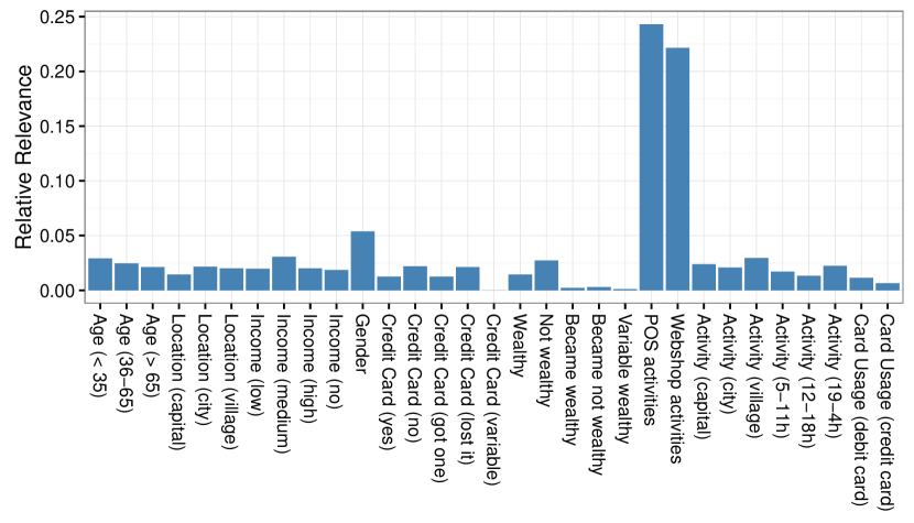
Figure 1: This plot visualizes the relative number of times a feature was chosen to build a tree in Task 2. The activity features are used in almost every fourth tree.

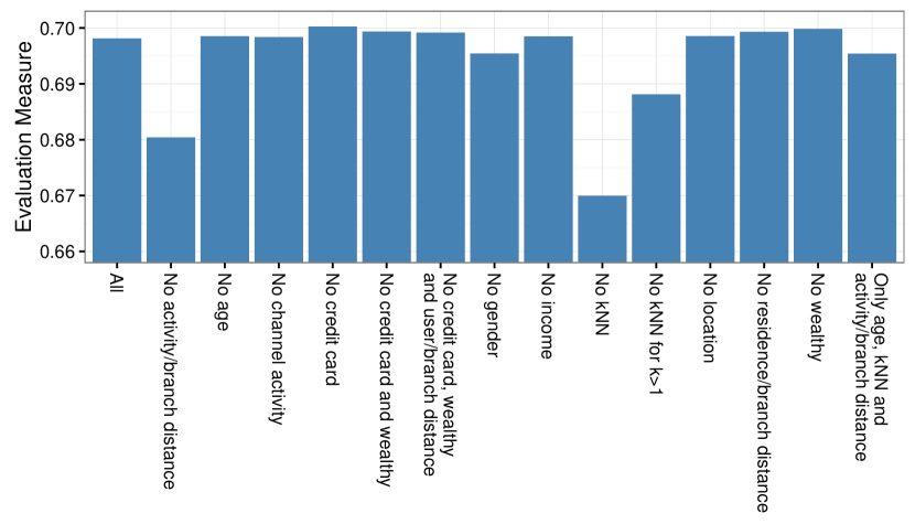
Figure 2: Intermediate feature backward selection results for Task 1. Location-aware features provide huge improvements.

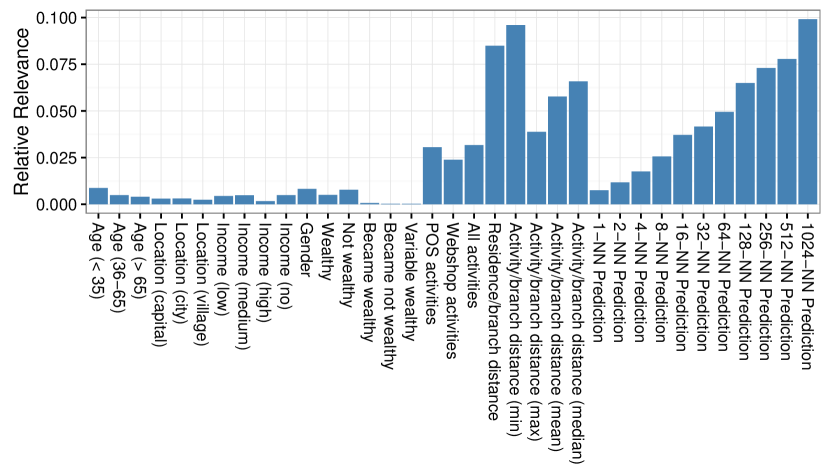
Figure 3: This plot visualizes the relative relevance of all features used in Task 1. The higher the score, the more often the feature was used for building a tree. Location-aware features prove to be highly predictive.

For Task 2 we considered location information about activities, bank branches and customers to be irrelevant and only used aforementioned features. However, for Task 1 this information was one of the most impactful information. One feature we used was the distance between the residence of the customer and a bank branch which is a quite obvious choice. Digging into the data, we saw that there were many customers using bank branches very far away from their residence. We tried to cover this by also adding the maximum, minimum, mean and median distance between a bank branch and the customer’s activities. Finally, we added k-nearest-neighbors predictions for $k=2^{0},2^{1},\ldots,2^{10}$ using the Euclidean distance between the residence of customers as the distance function. These features follow the simple assumption that customers that live nearby visit the same bank branches. Figure 2 provides insight into our intermediate feature selection experiments for Task 1 and clearly shows the importance of the location-aware features. Based on this experiment, we used all features but the credit card information for Task 1. Figure 3 shows the relative frequency of a specific feature being taken as a splitting variable. Again, this shows the importance of location-aware features for Task 1.

4 Hyperparameter Tuning and Ensembling

For both tasks we tuned the hyperparameters by considering the choice of hyperparameters $\boldsymbol{\lambda}$ as a black-box optimization problem

$$\underset{\boldsymbol{\lambda}}{\arg\min\ }\mathcal{L}\left(\hat{y}_{\boldsymbol{\lambda}}\left(D_{\text{valid}}\right),y_{\text{valid}}\right)$$ (2)

where $\hat{y}_{\boldsymbol{\lambda}}$ is the model that was trained on the training partition of the data $D_{\text{train}}$ using hyperparameter configuration $\boldsymbol{\lambda}$ and $\hat{y}_{\boldsymbol{\lambda}}\left(D_{\text{valid}}\right)$ the corresponding predictions for the validation partition $D_{\text{valid}}$. Then, the problem of hyperparameter tuning is to find a hyperparameter configuration $\boldsymbol{\lambda}$ such that a loss function $\mathcal{L}$ given the predictions and the groundtruth is minimized.

We tackled this black-box optimization problem using Sequential Model-based Optimization (SMBO) [3]. Figure 4 presents the progress of the optimization process that was conducted in parallel on 100 cores for our own train/validation split as well as results on the public leaderboard for Task 1.

For Task 2, we tried diverse ways of ensembling using different base models but did not achieve any improvement. In the end, we averaged the predictions of 100 models for the best hyperparameter configuration using different seeds.

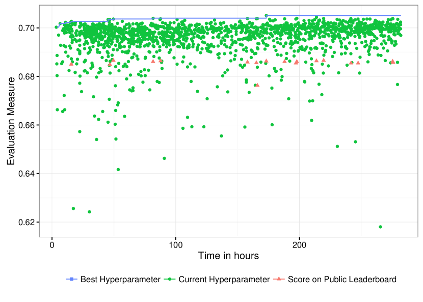
Figure 4: Searching for a good hyperparameter configuration with 100 cores in parallel. The public leaderboard score is shown for some of the best hyperparameter configurations on our validation set.

One of our best single models for Task 1 achieved a cosine@1 score of $0.676$ and a cosine@5 score of $0.728$ leading to an overall score of $0.702$ on our validation split. The performance on the test set is with $0.686$ much smaller. A possible reason might be temporal effects because the predictions for the test customers are for 2015 but we learn on data from 2014.

Table 1: The performance of the top five teams for both tasks on the public leaderboard.

Task 1			Task 2
Team	Score		Team	Score
1. ISMLL	0.68659		1. achm	0.71862
2. Ya	0.68512		2. Cosine Vinny	0.71730
3. Cosine Vinny	0.67436		3. Degrees of Freedom	0.71589
4. Outliers	0.65607		4. ISMLL	0.71523
5. seed71	0.65287		5. TwoBM	0.71479

5 Conclusions

Our solution is based on strong ensemble methods, smart feature engineering and an intense search for optimal hyperparameter configurations. For Task 1, this paid of leading to the best solution regarding the public leaderboard as well as a decent result for Task 2.

Acknowledgments.

The authors gratefully acknowledge the co-funding of their work by the German Research Foundation (DFG) under grant SCHM 2583/6-1.

References

- [1] ECML-PKDD 2016 Discovery Challenge on Bank Card Usage. https://dms.sztaki.hu/ecml-pkkd-2016/#/app/home (2016), [Online; accessed 8-July-2016]
- [2] Chen, T., Guestrin, C.: Xgboost: A scalable tree boosting system. In: The 22nd ACM SIGKDD International Conference on Knowledge Discovery and Data Mining, KDD ’16, San Francisco, CA, USA - August 13 - 17, 2016 (2016)
- [3] Snoek, J., Larochelle, H., Adams, R.P.: Practical bayesian optimization of machine learning algorithms. In: Advances in Neural Information Processing Systems 25: 26th Annual Conference on Neural Information Processing Systems 2012. Proceedings of a meeting held December 3-6, 2012, Lake Tahoe, Nevada, United States. pp. 2960–2968 (2012)