Supersymmetric spin chains with non-monotonic dispersion relation: criticality and entanglement entropy

Abstract

We study the critical behavior and the ground-state entanglement of a large class of $\mathrm{su}(1|1)$ supersymmetric spin chains with a general (not necessarily monotonic) dispersion relation. We show that this class includes several relevant models, with both short- and long-range interactions of a simple form. We determine the low temperature behavior of the free energy per spin, and deduce that the models considered have a critical phase in the same universality class as a $(1+1)$-dimensional conformal field theory (CFT) with central charge equal to the number of connected components of the Fermi sea. We also study the Rényi entanglement entropy of the ground state, deriving its asymptotic behavior as the block size tends to infinity. In particular, we show that this entropy exhibits the logarithmic growth characteristic of $(1+1)$-dimensional CFTs and one-dimensional (fermionic) critical lattice models, with a central charge consistent with the low-temperature behavior of the free energy. Our results confirm the widely believed conjecture that the critical behavior of fermionic lattice models is completely determined by the topology of their Fermi surface.

I Introduction

Integrable spin chains often provide a fertile ground for studying key theoretical concepts in a simple framework that captures the essential features of the problems under consideration. An important example of this assertion is the analysis of the entanglement of a quantum system, which can be considered as one of the fundamental characteristics of the quantum realm Horodecki et al. (2009). One of the most common ways of measuring the degree of entanglement of a state of a quantum system $X$ is via the bipartite entropy of a subsystem $A$ Nielsen and Chuang (2010). This entropy is defined by $S_{A}=S(\rho_{A})$, where $\rho_{A}=\operatorname{tr}_{X\setminus A}\rho$ is the reduced density matrix of the subsystem $A$, $\rho$ is the density matrix representing the state of the whole system, and $S$ is an appropriate entropy functional (von Neumann, Rényi, etc.). The small class of models for which the entanglement entropy can be evaluated in closed form (at least in the thermodynamic limit) includes certain integrable spin chains, like the Lipkin–Meshkov–Glick model Latorre et al. (2005), its $\mathrm{su}(n)$ generalization Carrasco et al. (2016a) and the nearest-neighbors Heisenberg $X\!X$ and $X\!Y$ models Vidal et al. (2003); Jin and Korepin (2004); Its et al. (2005). As is well known, the latter two models are critical (gapless) for a certain range of values of the applied magnetic field, their corresponding Virasoro algebras having central charge respectively equal to $1$ and $1/2$. In both cases, the bipartite Rényi entropy of a block of $L$ consecutive spins when the whole chain is in its ground state scales as $c(1+\alpha^{-1})(\log L)/6$ in the critical phase, where $\alpha$ is the Rényi parameter ($\alpha=1$ for the von Neumann entropy) and $c$ is the central charge. This behavior is consistent with the scaling of the Rényi entanglement entropy of a ($1+1$)-dimensional conformal field theory (CFT) Holzhey et al. (1994); Calabrese and Cardy (2004, 2005). In fact, the logarithmic scaling of the ground state entanglement entropy is a characteristic feature of critical (fermionic) one-dimensional lattice models with short-range interactions (see, e.g., Ref. Eisert et al. (2010)).

In a previous paper Carrasco et al. (2016b), we showed that the above results also apply to a large class of supersymmetric spin chains with general (not necessarily short-range) interactions, which turn out to be equivalent to a suitable free fermion model. The critical character of these chains (for appropriate values of the chemical potential $\mu$) was ascertained via the analysis of the low-temperature behavior of the free energy per spin. Indeed, we proved that when the dispersion relation ${\mathcal{E}}(p)$ of the corresponding free fermion model is monotonic in the interval $[0,\pi]$, for $0<\mu<{\mathcal{E}}(\pi)$ the free energy per spin is approximately given (in natural units $\hbar=k_{B}=1$) by

$$f(T)\simeq f_{0}-\frac{\pi cT^{2}}{6v}\,,$$ (1)

where $v$ is the Fermi velocity (or effective speed of “sound”) and $c=1$. This is precisely the expected behavior of the free energy for any critical model ($c$ being the central charge of its Virasoro algebra), since at low temperatures the free energy of a quantum system is determined by its lowest energy levels, and the free energy per spin of a ($1+1$)-dimensional CFT with central charge $c$ satisfies (1) for sufficiently small $T$ Blöte et al. (1986); Affleck (1986). We also studied the ground-state Rényi entanglement entropy of the above mentioned supersymmetric spin chains, showing that in the thermodynamic limit $L\to\infty$ it again behaves as that of a $(1+1)$-dimensional CFT with central charge $c=1$ .

The aim of this paper is to extend the results of Ref. Carrasco et al. (2016b) by suppressing the requirement that the dispersion relation be monotonic in $[0,\pi]$. As shown in Section III, this makes it possible to treat a host of naturally arising models, like supersymmetric spin chains with near and next-to-near interactions, or with long-range rational interactions, whose dispersion relation is not always monotonic. In fact, the entanglement entropy of fairly arbitrary energy eigenstates of one-dimensional free fermionic systems (in particular, of the ground state of such systems with a non-monotonic dispersion relation) has been previously studied in the literature; see, e.g., Refs. Alba et al. (2009); Ares et al. (2014a). In general, the entanglement entropy of the ground state of these models grows logarithmically with the size $L$ of the subsystem, with a constant prefactor determined by the number of boundary points of the Fermi “surface” in $[0,2\pi)$. This logarithmic scaling is a manifestation of the so-called “area law”, which is believed to hold for critical fermionic systems in an arbitrary number of dimensions Eisert et al. (2010). We shall show that the $\mathrm{su}(1|1)$ supersymmetric chains studied in this paper do indeed satisfy the area law. More precisely, by analyzing the low-temperature behavior of the free energy we shall first show that the models under consideration are critical for ${\mathcal{E}}_{\text{min}}<\mu<{\mathcal{E}}_{\text{max}}$, where ${\mathcal{E}}_{\text{min}}$ and ${\mathcal{E}}_{\text{max}}$ respectively denote the minimum and maximum values of the dispersion relation. (As explained in Section IV, strictly speaking this is only true if the roots of the equation ${\mathcal{E}}(p)=\mu$ are all simple.) From the latter analysis it also follows that the central charge of these models is equal to the number $m+1$ of disjoint intervals that make up the Fermi sea. We shall next study the ground state Rényi entanglement entropy, showing that in the thermodynamic limit $L\to\infty$ it behaves as $k_{\alpha}\log L+C_{\alpha}$. We shall explicitly compute the (non-universal) constant $C_{\alpha}$, and prove that the prefactor $k_{\alpha}$ is equal to $(m+1)(1+\alpha^{-1})/6$. This is in agreement with the value of the central charge deduced from the low-temperature analysis of the free energy, and once again confirms the conjecture that the entanglement properties of critical fermion models are entirely determined by the topology of their Fermi surface Eisert et al. (2010).

We shall end this section with a few words on the paper’s organization. In Section II we recall the definition of the supersymmetric chains under consideration and review their main properties. Section III is devoted to the analysis of the models’ dispersion relation and the construction of simple examples of supersymmetric chains, featuring both short- and long-range interactions, with a non-monotonic dispersion relation. In Section IV we derive the asymptotic behavior of the models’ free energy per spin at low temperature, showing that they are critical in an appropriate range of the chemical potential, and determine the central charge of the corresponding Virasoro algebra. The asymptotic behavior of the entanglement entropy of the models’ ground state is determined in Section V using a particular case of the Fisher–Hartwig conjecture for Toeplitz matrices Fisher and Hartwig (1968) rigorously proved by Böttcher and Silbermann Böttcher and Silbermann (1985). We briefly state our conclusions and outline several future developments suggested by the present work in Section VI. The paper ends with three appendices in which we present a review of the application of the Fisher–Hartwig conjecture in the present context, as well as the proofs of several technical results used throughout Section V.

II The models

The type of models we shall study in this work is the class of $\mathrm{su}(1|1)$ supersymmetric spin chains with translationally invariant interactions introduced in Ref. Carrasco et al. (2016b). In the latter models each site is occupied either by a scalar boson or a spinless fermion, whose creation operators we shall respectively denote by $b_{i}^{\dagger}$ and $f_{i}^{\dagger}$, the subindex $i=1,\dots,N$ indicating the site on which these operators act. Thus the Hilbert space is the $2^{N}$-dimensional subspace ${\mathfrak{H}}$ of the infinite-dimensional Fock space defined by the constraints

$$b_{i}^{\dagger}b_{i}+f_{i}^{\dagger}f_{i}=1\,,\qquad 1\leqslant i\leqslant N\,.$$ (2)

The Hamiltonian of the models under consideration is given by 

$$H=\sum_{i<j}h_{N}(j-i)(1-S_{ij})-\mu N_{f}\,,$$ (3)

where the operator $N_{f}$ is the total fermion number

$$N_{f}=\sum_{i}f_{i}^{\dagger}f_{i}\,,$$

so that the real parameter $\mu$ has the natural interpretation of the fermions’ chemical potential. The real-valued function $h_{N}(k)$ giving the strength of the interaction between two particles $k$ sites apart is assumed to satisfy the constraint

$$h_{N}(x)=h_{N}(N-x)\,,$$ (4)

but is otherwise arbitrary . In other words, the chain is closed, i.e, translationally invariant. Finally, $S_{ij}$ is the $\mathrm{su}(1|1)$ spin permutation operator, defined by Haldane (1994)

$$S_{ij}=b_{i}^{\dagger}b_{j}^{\dagger}b_{i}b_{j}+f_{i}^{\dagger}f_{j}^{\dagger}f_{i}f_{j}+f_{j}^{\dagger}b_{i}^{\dagger}f_{i}b_{j}+b_{j}^{\dagger}f_{i}^{\dagger}b_{i}f_{j}\,.$$

Equivalently, let $|s_{1},\dots,s_{N}\rangle\equiv|s_{1}\rangle\otimes\cdots\otimes|s_{N}\rangle$ (with $s_{k}\in\{0,1\}$) be a state of the canonical spin basis, where $|0\rangle$ and $|1\rangle$ respectively denote the state with one boson or one fermion. The action of $S_{ij}$ on the latter state is then given by

$$S_{ij}|\dots,s_{i},\dots,s_{j},\dots\rangle=(-1)^{n}|\dots,s_{j},\dots,s_{i},\dots\rangle\,,$$ (5)

where $n=s_{i}=s_{j}$ if $s_{i}=s_{j}$ while for $s_{i}\neq s_{j}$ $n$ equals the number of fermions in the state $|s_{1},\dots,s_{N}\rangle$ occupying the sites $i+1,\dots,j-1$. The operator $S_{ij}$ is clearly invariant under the supersymmetry transformation $b_{i}\leftrightarrow f_{i}$ ($1\leqslant i\leqslant N$), and on ${\mathfrak{H}}$ we have $N_{f}\mapsto N-N_{f}=N_{b}$, where $N_{b}=\sum_{i}b_{i}^{\dagger}b_{i}$ is the total boson number. Hence the Hamiltonian (3) is indeed supersymmetric-invariant, up to a constant term and the usual relabeling $\mu\mapsto-\mu$.

The fundamental feature of the $\mathrm{su}(1|1)$ supersymmetric chain (3), explained in detail in Refs. Carrasco et al. (2016b); Finkel and González-López (2014), is that it can be mapped into a free-fermion model by interpreting the boson state $|0\rangle$ as the fermion vacuum. More precisely, consider the operators

$$a_{i}^{\dagger}=f^{\dagger}_{i}b_{i}\,,\qquad i=1,\dots,N,$$

which can be regarded as a new set of fermion creation operators as they obviously satisfy the canonical anticommutation relations (CAR) on ${\mathfrak{H}}$. It was shown by Haldane Haldane (1994) that on ${\mathfrak{H}}$ the $\mathrm{su}(1|1)$ permutation operator $S_{ij}$ can be simply expressed as

$$S_{ij}=1-a^{\dagger}_{i}a_{i}-a^{\dagger}_{j}a_{j}+a^{\dagger}_{i}a_{j}+a^{\dagger}_{j}a_{i}\,.$$ (6)

Substituting into Eq. (3) we readily obtain

$$H=-\sum_{i\neq j}h_{N}(|i-j|)a^{\dagger}_{i}a_{j}-(\mu-\mu_{0})\sum_{i}a^{\dagger}_{i}a_{i},$$ (7)

where

$$\mu_{0}=\sum_{j=1}^{N-1}h_{N}(j)\,.$$

We thus see that the spin chain (3) is indeed equivalent to a free-fermion model with hopping amplitude $-h_{N}(|i-j|)$ and chemical potential $\mu-\mu_{0}$.

Since the Hamiltonian (7) is translationally invariant on account of Eq. (4), it can be diagonalized by the discrete Fourier transform

$$\hat{a}_{l}=\frac{1}{\sqrt{N}}\,\sum_{k=1}^{N}\mathrm{e}^{-2\pi\mathrm{i}kl/N}a_{k}\,,\qquad 0\leqslant l\leqslant N-1\,.$$ (8)

Indeed, the operators $\hat{a}_{l}$ obviously satisfy the CAR, and can therefore be considered as a new set of fermionic operators. Moreover, a straightforward calculation shows that Finkel and González-López (2014)

$$H=\sum_{l=0}^{N-1}\Big{(}\varepsilon_{N}(l)-\mu\Big{)}\hat{a}^{\dagger}_{l}\hat{a}_{l}\,,$$ (9)

where

$$\varepsilon_{N}(l)=\sum_{j=1}^{N-1}\big{[}1-\cos(2\pi jl/N)\big{]}h_{N}(j)\,.$$ (10)

Likewise, the system’s total momentum operator ${\mathcal{P}}$ is given by Basu-Mallick et al. (2008)

$${\mathcal{P}}=\sum_{l=0}^{N-1}p_{l}\,\hat{a}^{\dagger}_{l}\hat{a}_{l}\,,$$

with

$$p_{l}=\frac{2\pi l}{N}\quad(\bmod\ 2\pi)\,.$$

Thus the operator $\hat{a}^{\dagger}_{l}$ creates a (non-localized) fermion with well-defined energy $\varepsilon_{N}(l)$ and momentum $p_{l}$. It follows from Eq. (9) that the spectrum of $H$ is the set of numbers of the form

$$E_{N}(\delta_{0},\dots,\delta_{N-1})=\sum_{l=0}^{N-1}\delta_{l}\varepsilon_{N}(l)\,,$$

with $\delta_{l}\in\{0,1\}$, whose corresponding eigenstates are given by

$$\psi(\delta_{0},\dots,\delta_{N-1})=(\hat{a}_{0}^{\dagger})^{\delta_{0}}\cdots(\hat{a}_{N-1}^{\dagger})^{\delta_{N-1}}|0,\dots,0\rangle\,.$$

III The dispersion relation

An essential requirement making it possible to study the chain (3) —or, equivalently, its fermionic counterpart (7)— in the thermodynamic limit is the existence of a smooth function ${\mathcal{E}}(p)$ independent of $N$ such that when $N\to\infty$ we have

$$\varepsilon_{N}(Np/2\pi)={\mathcal{E}}(p)+o(1)\,.$$ (11)

When this is the case, we shall refer to ${\mathcal{E}}(p)$ as the model’s dispersion relation. From the latter equation and the identity $\varepsilon_{N}(l)=\varepsilon_{N}(N-l)$ it follows that the dispersion relation is always symmetric about $\pi$, namely

$${\mathcal{E}}(p)={\mathcal{E}}(2\pi-p)\,.$$ (12)

Likewise, $\varepsilon_{N}(0)=0$ implies that ${\mathcal{E}}(0)=0$ . It is also customary to extend ${\mathcal{E}}(p)$ to the whole real line as a $2\pi$-periodic function, in which case Eq. (12) entails that ${\mathcal{E}}(p)={\mathcal{E}}(-p)$.

For instance, for the $\mathrm{su}(1|1)$ Haldane–Shastry chain Haldane (1994), whose interaction strength is given by

$$h_{N}(x)=\frac{\pi^{2}/N^{2}}{\sin^{2}(\pi x/N)}\,,$$ (13)

it was shown in Ref. Göhmann and Wadati (1995) that

$$\varepsilon_{N}(l)=\frac{2\pi^{2}}{N^{2}}\,l(N-l)\,.$$

Hence in this case (11) holds with

$${\mathcal{E}}(p)=\frac{p}{2}\,(2\pi-p)$$ (14)

and no error term. In fact, it can be shown that Eq. (11) also holds (again with no error term) for a suitable dispersion relation ${\mathcal{E}}$ in the more general chain with elliptic interactions studied in Ref. Finkel and González-López (2014).

We shall next present a few relevant examples of models of the form (3) for which the dispersion relation is guaranteed to exist. To this end, it is convenient to rewrite Eq. (10) to take into account conditions (4), namely

$$\varepsilon_{N}(l)=2\sum_{j=1}^{\lfloor(N-1)/2\rfloor}\big{[}1-\cos(2\pi jl/N)\big{]}h_{N}(j)\\ +2[1-\pi(N)]\,\pi(l)\,h_{N}(N/2)\,,$$ (15)

where $\pi(k)\in\{0,1\}$ denotes the parity of the integer $k$ and $\lfloor x\rfloor$ is the integer part of $x\in{\mathbb{R}}$. Clearly, the values of $h_{N}(j)$ with $1\leqslant j\leqslant N/2$ appearing in the latter equation are no longer restricted by Eq. (4). For this reason, from now on we shall implicitly restrict the domain of $h_{N}$ to the range $1\leqslant j\leqslant N/2$, since for $N/2<j\leqslant N-1$ we simply have $h_{N}(j)=h_{N}(N-j)$. In this vein, we shall say (with a slight abuse of language) that the interaction is independent of $N$ if there is a fixed function $h(x)$ such that $h_{N}(j)=h(j)$ for $1\leqslant j\leqslant N/2$ . If this is the case we shall simply write $h_{N}=h$, again implicitly assuming that we are restricting ourselves to the range $1\leqslant j\leqslant N/2$.

An important class of models of the form (3) for which the dispersion relation ${\mathcal{E}}(p)$ is guaranteed to exist are those whose interaction strength $h_{N}$ is short-ranged and independent of $N$. By this we mean that there is a positive integer $r$ (the range of the interaction) such that $h_{N}(j)=0$ for $r<j<N-r$, and

$$h_{N}(j)=\alpha_{j}\,,\qquad 1\leqslant j\leqslant r\,,$$ (16)

with $\alpha_{j}$ independent of $N$ and $\alpha_{r}\neq 0$. Obviously, in this case we have

$${\mathcal{E}}(p)=2\sum_{j=1}^{r}\alpha_{j}\big{[}1-\cos(jp)\big{]}\,.$$ (17)

In fact, the same is true if we drop (16) but assume instead that the limit

$$\lim_{N\to\infty}h_{N}(j)\equiv\alpha_{j}$$

exists for all $j=1,\dots,r$ .

On the other hand, the short range of the interaction $h_{N}$ is by no means a necessary condition for the existence of the dispersion relation ${\mathcal{E}}(p)$. Indeed, suppose for simplicity that $h_{N}=h$ is independent of $N$, and that the series $\sum_{j=1}^{\infty}h(j)$ is absolutely convergent. Then (11) clearly holds with

$${\mathcal{E}}(p)=2\sum_{j=1}^{\infty}h(j)\big{[}1-\cos(jp)\big{]}\,.$$ (18)

For instance, for the power law interaction $h_{N}(x)=Cx^{-\nu}$ with $\nu>1$ the previous series can be summed in closed form in terms of the polylogarithm function Olver et al. (2010)

$$\operatorname{Li}_{\nu}(z)=\sum_{j=1}^{\infty}\frac{z^{j}}{j^{\nu}}\,,\qquad|z|\leqslant 1\,,$$

namely (taking, for simplicity, $C=1$)

$${\mathcal{E}}(p)=2\zeta(\nu)-\operatorname{Li}_{\nu}(\mathrm{e}^{\mathrm{i}p})-\operatorname{Li}_{\nu}(\mathrm{e}^{-\mathrm{i}p})\\ =2\big{[}\zeta(\nu)-\operatorname{Re}\operatorname{Li}_{\nu}(\mathrm{e}^{\mathrm{i}p})\big{]},$$ (19)

where $\zeta$ denotes Riemann’s zeta function (cf. Fig. 1).

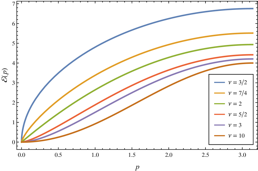
Figure 1: Dispersion relation of the $\mathrm{su}(1|1)$ chain (3) with power-law interaction $h_{N}(x)=x^{-\nu}$ for several values of the exponent $\nu$ between $3/2$ and $10$.

From the integral representation

$$\operatorname{Li}_{\nu}(z)=\frac{z}{\Gamma(\nu)}\int_{0}^{\infty}\frac{x^{\nu-1}}{\mathrm{e}^{x}-z}\,\mathrm{d}x\,,$$ (20)

where $\Gamma$ is Euler’s gamma function, we obtain the equivalent expression

$${\mathcal{E}}(p)=2\zeta(\nu)-\frac{2}{\Gamma(\nu)}\int_{0}^{\infty}\frac{(\mathrm{e}^{x}\cos p-1)x^{\nu-1}}{\mathrm{e}^{2x}-2\mathrm{e}^{x}\cos p+1}\,\mathrm{d}x\,.$$ (21)

Using the latter formula in the identity ${\mathcal{E}}(p)=\int_{0}^{p}{\mathcal{E}}^{\prime}(t)\mathrm{d}t$ and reversing the order of integration we arrive at the somewhat simpler expression

$${\mathcal{E}}(p)=\frac{2^{\nu}s}{\Gamma(\nu)}\,\int_{0}^{\infty}\frac{x^{\nu-1}\coth x}{\sinh^{2}x+s}\,\mathrm{d}x\,,\quad s\equiv\sin^{2}(p/2)\,.$$

Remarkably, for $\nu=2$ Eq. (19) reduces to Eq. (14) (see, e.g., Olver et al. (2010)). Thus the $\mathrm{su}(1|1)$ chain with rational interaction $h_{N}(x)=x^{-2}$ has the same dispersion relation as the Haldane–Shastry chain (13). This is of course not entirely unexpected, since for fixed $x\neq 0$ we have $\lim_{N\to\infty}(\pi/N)^{2}\sin^{-2}(\pi x/N)=x^{-2}$. Note, however, that for $x\sim N/2$ both interactions, although negligibly small as $N\to\infty$, differ by a factor${}\sim(\pi/2)^{2}$ (cf. Fig. 2).

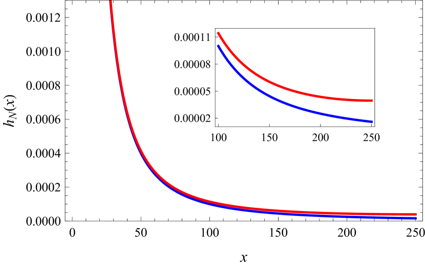
Figure 2: Comparison of the interaction strength (13) of the $\mathrm{su}(1|1)$ HS chain (red) with the simple inverse-square law $h_{N}(x)=1/x^{2}$ (blue) for $N=500$. Inset: same plot for the range $100\leqslant x\leqslant 250$.

Of course, although (11) holds for a wide range of interesting interactions, it is not universally true. For instance, it is not satisfied by the $N$-independent interaction $h_{N}(x)=C/x$, since

$$\sum_{j=1}^{\infty}\frac{\cos(jp)}{j}=-\log\bigl{(}2\sin(p/2)\bigr{)}$$

converges for $0<p<2\pi$ while the series $\sum_{j=1}^{\infty}j^{-1}$ is divergent.

In a previous paper Carrasco et al. (2016b) we analyzed the critical behavior of supersymmetric spin chains of the type (3) whose dispersion relation is monotonic in the interval $[0,\pi]$. These models include the $\mathrm{su}(1|1)$ Haldane–Shastry chain (cf. (14)) and, more generally, its elliptic generalization introduced in Ref. Finkel and González-López (2014). As is apparent from Fig. 1 (and can be analytically checked differentiating Eq. (21)), the chain (3) with power-law interactions also exhibits this property. However, this behavior is not universal, and there are in fact simple examples of supersymmetric chains of the form (3) with a non-monotonic dispersion relation.

Indeed, consider to begin with the chain (3) with nearest and next-to-nearest interactions, whose Hamiltonian (up to an irrelevant multiplicative constant) is given by

$$H=\sum_{i}(1-S_{i,i+1})+J\sum_{i}(1-S_{i,i+2})-\mu N_{f}\,,$$ (22)

with $S_{N,N+1}\equiv S_{1N}$, $S_{N-1,N+1}\equiv S_{1,N-1}$ and $S_{N,N+2}\equiv S_{2N}$ . Note that when $J=0$ the fermionic version of the latter model can be mapped to the (closed) Heisenberg $X\!X$ chain by a Wigner–Jordan transformation Carrasco et al. (2016b). From Eq. (15) with $h_{N}(1)=1$ and $h_{N}(2)=J$ we easily obtain

$${\mathcal{E}}(p)=2(1-\cos p)+2J(1-\cos 2p)\,.$$

Since

$${\mathcal{E}}^{\prime}(p)=2\sin p(1+4J\cos p)\,,$$

the dispersion relation will have a critical point in $(0,\pi)$ if and only if $|J|>1/4$ (more precisely, a maximum for $J>1/4$ and a minimum for $J<-1/4$). Thus in this case the dispersion relation is not monotonic in $[0,\pi]$ provided that $|J|>1/4$ . The same is clearly true for chains of the form (3) with interactions of finite range $r>1$, for suitable values of the interaction strengths.

It is also easy to construct simple examples of chains of the form (3) with long-range interactions with a non-monotonic dispersion relation. Take, for instance,

$$h_{N}(x)=\frac{1}{x^{2}}-\frac{J}{x^{3}}\,,$$ (23)

whose dispersion relation is given by

$${\mathcal{E}}(p)=\frac{p}{2}\,(2\pi-p)-2J\big{[}\zeta(3)-\operatorname{Re}\operatorname{Li}_{3}(\mathrm{e}^{\mathrm{i}p})\big{]}\,.$$

If $p\in(0,\pi)$, differentiating the latter equation we obtain

$${\mathcal{E}}^{\prime}(p)=(\pi-p)[1-J\varphi(p)]\,,$$

with

$$\varphi(p)=2\operatorname{Im}\operatorname{Li}_{2}(\mathrm{e}^{\mathrm{i}p})/(\pi-p)\,.$$ (24)

It can be shown (cf. Fig. 3) that the function $\varphi(p)$ increases monotonically over the interval $(0,\pi)$, with $\varphi(0)=0$ and $\lim_{p\to\pi-0}\varphi(p)=2\log 2$ , so that ${\mathcal{E}}^{\prime}(p)$ changes sign once (from positive to negative) in $(0,\pi)$ if and only if $J>(2\log 2)^{-1}$. We conclude that the dispersion relation of the chain (3) with interaction (23) is not monotonic on $[0,\pi]$ provided that $J>(2\log 2)^{-1}\simeq 0.721348$. In particular, for $(2\log 2)^{-1}<J<1$ the dispersion relation is not monotonic in $[0,\pi]$ even if the interaction strength is positive for $x\geqslant 1$ (see Fig. 3 for a plot of ${\mathcal{E}}(p)$ when $J=0.9$).

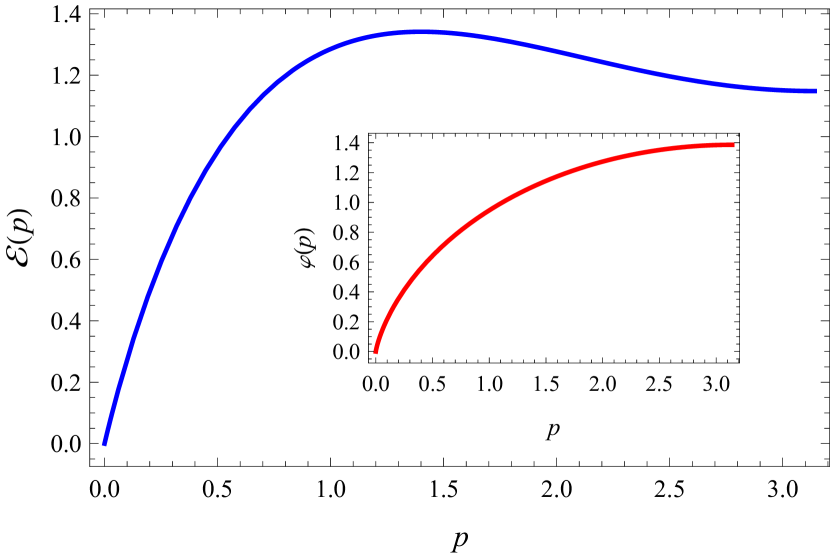
Figure 3: Dispersion relation of the spin chain (3) with interaction (23) for $J=0.9$. Inset: plot of the function $\varphi(p)$ in Eq. (24).

IV Critical behavior

In this section we shall study the critical properties of the spin chain (3) when its dispersion relation ${\mathcal{E}}(p)$ is not necessarily monotonic over the interval $[0,\pi]$. To this end, we shall examine the low temperature behavior of the Helmholtz free energy per spin

$$f(T)=-T\lim_{N\to\infty}\frac{\log Z_{N}}{N}\,,$$

which for this model is given by (cf. Carrasco et al. (2016b))

$$f(T)=-\frac{T}{\pi}\int_{0}^{\pi}\log\bigl{[}1+\mathrm{e}^{-\beta({\mathcal{E}}(p)-\mu)}\bigr{]}\,\mathrm{d}p\,.$$ (25)

In the previous expressions $Z_{N}$ denotes the partition function of the chain (3) with $N$ spins, and $\beta=1/T$ (in natural units $\hbar=k_{B}=1$). As remarked in the Introduction, at low temperatures the free energy of a critical model should satisfy Eq. (1). Moreover, it was shown in Ref. Carrasco et al. (2016b) that when ${\mathcal{E}}(p)$ is monotonic and nonnegative in the interval $[0,\pi]$ the model (3) is critical when the chemical potential $\mu$ lies in the interval $(0,{\mathcal{E}}(\pi))$, with central charge $c=1$, and noncritical for $\mu$ outside the closed interval $[0,{\mathcal{E}}(\pi)]$. We shall next extend this result to the more general case in which ${\mathcal{E}}(p)$ is not necessarily monotonic (nor nonnegative) in $[0,\pi]$.

To begin with, it is immediate to show that the model (3) is not critical when $\mu$ lies outside the interval $[{\mathcal{E}}_{\text{min}},{\mathcal{E}}_{\text{max}}]$. Indeed, suppose first that $\mu<{\mathcal{E}}_{\text{min}}$, so that ${\mathcal{E}}(p)-\mu>0$, $f_{0}\equiv f(0)=0$ and

$$|f(T)|<\frac{T}{\pi}\int_{0}^{\pi}\mathrm{e}^{-\beta({\mathcal{E}}(p)-\mu)}\,\mathrm{d}p<T\mathrm{e}^{-\beta({\mathcal{E}}_{\text{min}}-\mu)}\,,$$

in contradiction with the asymptotic behavior (1) characteristic of a critical model. Similarly, when $\mu>{\mathcal{E}}_{\text{max}}$ we have

$$f_{0}\equiv f(0)=\frac{1}{\pi}\int_{0}^{\pi}\big{[}{\mathcal{E}}(p)-\mu\big{]}\mathrm{d}p$$

and

$$|f(T)-f_{0}| =\frac{T}{\pi}\int_{0}^{\pi}\log\bigl{[}1+\mathrm{e}^{-\beta(\mu-{\mathcal{E}}(p))}\bigr{]}\,\mathrm{d}p$$

$$<T\mathrm{e}^{-\beta(\mu-{\mathcal{E}}_{\text{max}})}\,,$$

again in disagreement with Eq. (1). This conclusion is also borne out by the fact that when $\mu>{\mathcal{E}}_{\text{max}}$ or $\mu<{\mathcal{E}}_{\text{min}}$ the spectrum is clearly gapped, with energy gap respectively equal to $\mu-{\mathcal{E}}_{\text{max}}$ or ${\mathcal{E}}_{\text{min}}-\mu$.

Let us now consider the more interesting case in which $\mu\in({\mathcal{E}}_{\text{min}},{\mathcal{E}}_{\text{max}})$, in which the spectrum is clearly gapless. We shall suppose that the equation ${\mathcal{E}}(p)=\mu$ has $m+1\geqslant 1$ roots $p_{0}<p_{1}<\dots<p_{m}$ in the interval $(0,\pi)$, which we will assume to be simple. We start by expressing the free energy as

$$f(T)=f_{0}-\frac{T}{\pi}\int_{0}^{\pi}\log\bigl{(}1+\mathrm{e}^{-\beta|{\mathcal{E}}(p)-\mu|}\bigr{)}\mathrm{d}p\,,$$ (26)

where

$$f_{0}\equiv f(0)=\frac{1}{\pi}\int_{{\mathcal{E}}(p)<\mu}[{\mathcal{E}}(p)-\mu]\mathrm{d}p$$

and the last integral is extended to the subset of the interval $[0,\pi]$ defined by the inequality ${\mathcal{E}}(p)<\mu$. Clearly, as $T\to 0+$ the main contribution to the integral in Eq. (26) comes from an increasingly small neighborhood of the “turning points” $p_{i}$, near which $|{\mathcal{E}}(p)-\mu|$ is small. To exploit this fact, we choose $\Delta p>0$ small enough that $[p_{i}-\Delta p,p_{i}+\Delta p]\cap[p_{j}-\Delta p,p_{j}+\Delta p]=\emptyset$ for $i\neq j$ and ${\mathcal{E}}^{\prime}(p)\neq 0$ on $\cup_{i=0}^{m}[p_{i}-\Delta p,p_{i}+\Delta p]$. This is certainly possible, since by hypothesis ${\mathcal{E}}^{\prime}(p_{i})\neq 0$ for all $i$. Obviously, $\Delta p$ depends only on the dispersion relation ${\mathcal{E}}(p)$, and is therefore independent of $T$. Calling $A=[0,\pi]-\cup_{i=0}^{m}[p_{i}-\Delta p,p_{i}+\Delta p]$ we have

$$\int_{0}^{\pi}\log\bigl{[}1+\mathrm{e}^{-\beta|{\mathcal{E}}(p)-\mu|}\bigr{]}\mathrm{d}p=\int_{A}\log\bigl{[}1+\mathrm{e}^{-\beta|{\mathcal{E}}(p)-\mu|}\bigr{]}\mathrm{d}p\\ +\sum_{i=0}^{m}\int_{p_{i}-\Delta p}^{p_{i}+\Delta p}\log\bigl{[}1+\mathrm{e}^{-\beta|{\mathcal{E}}(p)-\mu|}\bigr{]}\mathrm{d}p\,.$$ (27)

The first integral can be easily estimated. Indeed, let $a$ be the minimum value of $|{\mathcal{E}}(p)-\mu|$ on the compact set $\overline{A}$, which is clearly positive since ${\mathcal{E}}(p)\neq\mu$ on $\overline{A}$, and denote by $|A|$ the length of $A$. We then have

$$\int_{A}\log\bigl{[}1+\mathrm{e}^{-\beta|{\mathcal{E}}(p)-\mu|}\bigr{]}\mathrm{d}p\leqslant\mathrm{e}^{-a\beta}|A|\leqslant\pi\mathrm{e}^{-a\beta}\,,$$ (28)

with $a$ (and $|A|$) obviously independent of $T$. Consider next the integral

$$I_{i}\equiv\int_{p_{i}-\Delta p}^{p_{i}+\Delta p}\log\bigl{[}1+\mathrm{e}^{-\beta|{\mathcal{E}}(p)-\mu|}\bigr{]}\mathrm{d}p\,.$$ (29)

To analyze its low temperature behavior, we perform the change of variable

$$x=\beta|{\mathcal{E}}(p)-\mu|$$ (30)

separately in each of the intervals $[p_{i}-\Delta p,p_{i}]$ and $[p_{i},p_{i}+\Delta p]$. Since ${\mathcal{E}}^{\prime}(p_{i})\neq 0$, this change of variable is one to one and $C^{\infty}$ in both of the latter intervals, and we have

$$\frac{I_{i}}{T}=\int_{0}^{\beta|{\mathcal{E}}(p_{i}-\Delta p)-\mu|}\log\bigl{(}1+\mathrm{e}^{-x}\bigr{)}\,\frac{\mathrm{d}x}{|{\mathcal{E}}^{\prime}(p)|}\\ +\int_{0}^{\beta|{\mathcal{E}}(p_{i}+\Delta p)-\mu|}\log\bigl{(}1+\mathrm{e}^{-x}\bigr{)}\,\frac{\mathrm{d}x}{|{\mathcal{E}}^{\prime}(p)|}\,.$$ (31)

The asymptotic behavior of these integrals as $T\to 0+$ can be easily determined taking into account that by construction ${\mathcal{E}}^{\prime}(p)$ does not vanish on both intervals $[p_{i}-\Delta p,p_{i}]$ and $[p_{i},p_{i}+\Delta p]$, and therefore

$$\frac{1}{{\mathcal{E}}^{\prime}(p)}=\frac{1}{{\mathcal{E}}^{\prime}(p_{i})}+O(p-p_{i})=\frac{1}{{\mathcal{E}}^{\prime}(p_{i})}+O(Tx)\,,$$

as $x(p_{i})=0$ implies that $p-p_{i}=O(Tx)$. Since the integral $\int_{0}^{\infty}x\log(1+\mathrm{e}^{-x})\mathrm{d}x$ is convergent we have

$$I_{i}=\frac{T}{v_{i}}\bigg{(}\int_{0}^{\beta|{\mathcal{E}}(p_{i}-\Delta p)-\mu|}\log\bigl{(}1+\mathrm{e}^{-x}\bigr{)}\mathrm{d}x\\ +\int_{0}^{\beta|{\mathcal{E}}(p_{i}+\Delta p)-\mu|}\log\bigl{(}1+\mathrm{e}^{-x}\bigr{)}\mathrm{d}x\bigg{)}+O(T^{2})\,,$$ (32)

where we have set

$$v_{i}=|{\mathcal{E}}^{\prime}(p_{i})|\,.$$

Moreover, if $K$ is independent of $\beta$ we have

$$\bigg{|}\int_{0}^{K\beta}\log\bigl{(}1+\mathrm{e}^{-x}\bigr{)}\mathrm{d}x-\int_{0}^{\infty}\log\bigl{(}1+\mathrm{e}^{-x}\bigr{)}\mathrm{d}x\bigg{|}\\ \leqslant\int_{K\beta}^{\infty}\mathrm{e}^{-x}\mathrm{d}x=\mathrm{e}^{-K\beta}.$$

Using this inequality and the integral

$$\int_{0}^{\infty}\log\bigl{(}1+\mathrm{e}^{-x}\bigr{)}\mathrm{d}x=\frac{\pi^{2}}{12}$$

in Eq. (32) we thus have

$$I_{i}=\frac{\pi^{2}T}{6v_{i}}+O(T^{2})\,.$$

From Eqs. (26)–(29) we finally obtain the asymptotic estimate

$$f=f_{0}-\frac{\pi T^{2}}{6}\sum_{i=0}^{m}\frac{1}{v_{i}}+O(T^{3})\,,\qquad T\to 0+\,.$$ (33)

This is the low temperature behavior of the free energy of a $(1+1)$-dimensional CFT with $m+1$ free bosons with Fermi velocities $v_{0},\dots,v_{m}$. Thus in this case the model (3) is critical, with central charge $c=m+1$.

The situation is markedly different if any of the roots of the equation ${\mathcal{E}}(p)=\mu$ is not simple. Indeed, assume that $p_{k}$ is a root of order $\nu_{k}>1$ of the latter equation, so that we can write

$${\mathcal{E}}(p)-\mu=\varepsilon_{k}\bigg{(}\frac{p-p_{k}}{b_{k}}\bigg{)}^{\nu_{k}}+O\bigl{[}(p-p_{k})^{\nu_{k}+1}\bigr{]}$$

with

$$b_{k}=\bigg{(}\frac{\nu_{k}!}{\big{|}{\mathcal{E}}^{(\nu_{k})}(p_{k})\big{|}}\bigg{)}^{1/\nu_{k}}\,,\qquad\varepsilon_{k}=\operatorname{sgn}{\mathcal{E}}^{(\nu_{k})}(p_{k})\,.$$

We now choose $\Delta p>0$ such that $[p_{i}-\Delta p,p_{i}+\Delta p]\cap[p_{j}-\Delta p,p_{j}+\Delta p]=\emptyset$ for $i\neq j$ and ${\mathcal{E}}^{\prime}(p)\neq 0$ on $[p_{i}-\Delta p,p_{i})\cup(p_{i},p_{i}+\Delta p]$ for all $i$. Proceeding as before we again arrive at Eqs. (26)-(27) and obtain the estimate (28) for the first integral in Eq. (27). In order to analyze the low temperature behavior of the integral $I_{k}$, we again perform the change of variable (30) in each of the intervals $[p_{k}-\Delta p,p_{k}]$ and $[p_{k},p_{k}+\Delta p]$, thus obtaining Eq. (31) with $i=k$. In each of the latter intervals we now have

$$|p-p_{k}|=b_{k}(Tx)^{1/\nu_{k}}\big{[}1+O\bigl{(}(Tx)^{1/\nu_{k}}\bigr{)}\big{]}$$

and

$$|{\mathcal{E}}^{\prime}(p)|=\frac{\nu_{k}}{b_{k}}\bigg{(}\frac{|p-p_{k}|}{b_{k}}\bigg{)}^{\nu_{k}-1}\big{[}1+O(p-p_{k})\big{]}\,,$$

so that

$$|{\mathcal{E}}^{\prime}(p)|^{-1}=\frac{b_{k}}{\nu_{k}}\,(Tx)^{1/\nu_{k}-1}\big{[}1+O\bigl{(}(Tx)^{1/\nu_{k}}\bigr{)}\big{]}\,.$$

Substituting into Eq. (31) and proceeding as before we easily obtain

$$I_{k} =\frac{2b_{k}}{\nu_{k}}\,T^{1/\nu_{k}}\!\int_{0}^{\infty}\!x^{1/\nu_{k}-1}\log\bigl{(}1+\mathrm{e}^{-x}\bigr{)}\mathrm{d}x+O\bigl{(}T^{2/\nu_{k}}\bigr{)}$$

$$=2b_{k}\big{(}1-2^{-1/\nu_{k}}\big{)}\Gamma\bigl{(}1+\nu_{k}^{-1}\bigr{)}\zeta\bigl{(}1+\nu_{k}^{-1}\bigr{)}T^{1/\nu_{k}}$$

$$\hphantom{2b_{k}\big{(}1-2^{-1/\nu_{k}}\big{)}\Gamma\bigl{(}1+\nu_{k}^{-1}\bigr{)}\zeta\bigl{(}1+\nu_{k}^{-1}\bigr{)}}+O\bigl{(}T^{2/\nu_{k}}\bigr{)}$$

(see Ref. Carrasco et al. (2016b) for more details on the evaluation of the last integral). Thus at low temperatures the contribution of $p_{k}$ to the free energy, given by

$$-\frac{TI_{k}}{\pi}=-\frac{2b_{k}}{\pi}\big{(}1-2^{-1/\nu_{k}}\big{)}\Gamma\bigl{(}1+\nu_{k}^{-1}\bigr{)}\zeta\bigl{(}1+\nu_{k}^{-1}\bigr{)}T^{1+1/\nu_{k}}\\ +O\bigl{(}T^{1+2/\nu_{k}}\bigr{)}\,,$$ (34)

dominates over the $O(T^{2})$ contribution coming from the simple roots $p_{i}$. Moreover, since the coefficient of $T^{1+1/\nu_{k}}$ in Eq. (34) is always negative, this term cannot be compensated by similar terms in Eq. (27) coming from other multiple roots. We thus conclude that when $\mu\in({\mathcal{E}}_{\text{min}},{\mathcal{E}}_{\text{max}})$, but the equation ${\mathcal{E}}(p)=\mu$ has at least one multiple root, the model (3) cannot be critical. A similar analysis shows that this is also the case when $\mu={\mathcal{E}}_{\text{min}}$ or $\mu={\mathcal{E}}_{\text{max}}$ . This shows that the model (3) is critical if and only if ${\mathcal{E}}_{\text{min}}<\mu<{\mathcal{E}}_{\text{max}}$ and all the roots of the equation ${\mathcal{E}}(p)=\mu$ are simple. When that is the case, the central charge of the model is equal to the number of connected components of its Fermi sea (or, equivalently, half the number of connected components of its Fermi “surface”). Thus, the universality class of the model (3) depends exclusively on the topology of its Fermi sea, which confirms the general assertion in Ref. Eisert et al. (2010).

V Ground state entanglement entropy

As mentioned in the Introduction, one of the hallmarks of a critical fermionic lattice model in one dimension with short-range interactions is the logarithmic growth of its ground state bipartite entanglement entropy with the length $L$ of the block of spins considered. More precisely, let

$$S_{\alpha}=(1-\alpha)^{-1}\log\operatorname{tr}(\rho_{L}^{\alpha})$$

denote the Rényi entropy of the block when the whole chain is in its ground state $|\psi\rangle$, where $\rho_{L}=\operatorname{tr}_{N-L}|\psi\rangle\langle\psi|$. The expected behavior of $S_{\alpha}$ in this type of models is then

$$S_{\alpha}=\frac{c}{6}\,(1+\alpha^{-1})\log L+C_{\alpha}\,,$$ (35)

where $c$ is the central charge of the corresponding Virasoro algebra and $C_{\alpha}$ is a non-universal constant (independent of $L$). We showed in a previous paper Carrasco et al. (2016b) that the latter formula is also valid for the supersymmetric chains (3) when their dispersion relation is monotonic (and nonnegative) in the interval $[0,\pi]$, even in the case of long-range interactions. In this section we shall extend this result to a general model of the type (3), whose dispersion relation need not be monotonic (or nonnegative) in $[0,\pi]$.

To this end, recall first of all that the ground state entanglement entropy $S_{\alpha}$ can be expressed in terms of the eigenvalues of the ground state correlation matrix $A_{L}$, with matrix elements

$$(A_{L})_{jk}=\langle\psi|a_{j}^{\dagger}a_{k}|\psi\rangle\,,\qquad 1\leqslant j,k\leqslant L\,.$$

Indeed, it was shown in Ref. Vidal et al. (2003) that

$$S_{\alpha}=\sum_{i=1}^{L}s_{\alpha}(\lambda_{i})\,,$$ (36)

where

$$s_{\alpha}(x)=(1-\alpha)^{-1}\log\biggl{[}\bigg{(}\frac{1+x}{2}\bigg{)}^{\alpha}+\bigg{(}\frac{1-x}{2}\bigg{)}^{\alpha}\biggr{]}$$

and $\lambda_{1},\dots,\lambda_{L}\in[-1,1]$ are the eigenvalues of the matrix $2A_{L}-\openone$. The asymptotic behavior of $S_{\alpha}$ can be determined following the method developed by Jin and Korepin Jin and Korepin (2004) for the $X\!X$ model. To this end, for $\varepsilon>0$ we define the complex-valued function

$$s^{(\varepsilon)}_{\alpha}(z)=(1-\alpha)^{-1}\log\biggl{[}\bigg{(}\frac{1+\varepsilon+z}{2}\bigg{)}^{\alpha}+\bigg{(}\frac{1+\varepsilon-z}{2}\bigg{)}^{\alpha}\biggr{]}\,,$$ (37)

where $\log z\equiv\log|z|+\mathrm{i}\arg_{(-\pi,\pi]}z$ and $z^{a}\equiv\mathrm{e}^{a\log z}$. This function has a logarithmic branch cut on the set $|\operatorname{Re}z|\geqslant 1+\varepsilon$ and no other singularities on a sufficiently small open subset (independent of $\varepsilon$) containing the interval $[-1,1]$ . By Cauchy’s theorem and Eq. (36), if $\gamma_{\varepsilon,\delta}$ is the path sketched in Fig. 4 we therefore have

$$S_{\alpha}=\lim_{\varepsilon,\delta\to 0+}\frac{1}{2\pi\mathrm{i}}\int_{\gamma_{\varepsilon,\delta}}s^{(\varepsilon)}_{\alpha}(\lambda)\frac{\mathrm{d}}{\mathrm{d}\lambda}\log D_{L}(\lambda)\,\mathrm{d}\lambda\,,$$ (38)

where

$$D_{L}(\lambda)\equiv\det(\lambda+1-2A_{L})\,.$$ (39)

As explained in Appendix A, the latter integral can then be approximated using a proved case of the Fisher–Hartwig conjecture to estimate the logarithmic derivative of $D_{L}(\lambda)$.

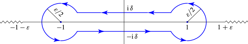
Figure 4: Integration path $\gamma_{\varepsilon,\delta}$ in Eq. (38).

V.1 Asymptotic formula for $D_{L}(\lambda)$

In order to derive the asymptotic behavior of $D_{L}(\lambda)$, we first need to determine the symbol of the Toeplitz matrix $T_{L}\equiv\lambda+1-2A_{L}$ (see again Appendix A for the definition of the symbol and its calculation in two simple cases). We shall compute this symbol for a general model of the type (3), whose dispersion relation is not assumed to be monotonic over $[0,\pi]$. More precisely, we shall only suppose that the equation ${\mathcal{E}}(p)=\mu$ has $m+1\geqslant 1$ simple roots $p_{0}<p_{1}<\dots<p_{m}$ in the interval $(0,\pi)$. From the symmetry of ${\mathcal{E}}$ around $\pi$ (cf. Eq. (12)) it then follows that the remaining roots of the equation ${\mathcal{E}}(p)=\mu$ in the interval $(0,2\pi)$ are $2\pi-p_{m}<\dots<2\pi-p_{1}<2\pi-p_{0}$.

In general, the system’s ground state $|\psi\rangle$ is determined by the conditions 

$$\left\{\begin{aligned} \hat{a}^{\dagger}_{k}|\psi\rangle&=0\,,\qquad\varepsilon_{N}(k)<\mu\,,\\[3.0pt] \hat{a}_{k}|\psi\rangle&=0\,,\qquad\varepsilon_{N}(k)>\mu\,,\end{aligned}\right.$$

so that

$$\langle\psi|\hat{a}_{j}^{\dagger}\hat{a}_{k}|\psi\rangle=\begin{cases}0\,,\quad&\varepsilon_{N}(k)>\mu\,,\\ \delta_{jk}\,,&\varepsilon_{N}(k)<\mu\,.\end{cases}$$

It immediately follows from Eq. (8) that the matrix elements of the correlation matrix $A_{L}$ are given by

$$(A_{L})_{jk}=\frac{1}{N}\sum_{l\in I}\mathrm{e}^{-2\pi\mathrm{i}(j-k)l/N}\,,$$

where the sum ranges over the set $I$ of integers in the range $[0,N-1]$ satisfying the condition $\varepsilon_{N}(l)<\mu$ . In the thermodynamic limit $N\to\infty$ the latter formula becomes

$$(A_{L})_{jk}=\frac{1}{2\pi}\int_{{\mathcal{E}}(p)<\mu}\mathrm{e}^{-\mathrm{i}(j-k)p}\mathrm{d}p\,,$$ (40)

where the integral is extended to the subset of the interval $(0,2\pi)$ defined by the inequality ${\mathcal{E}}(p)<\mu$. In fact, by the $2\pi$-periodicity of the integrand we can replace the interval $(0,2\pi)$ by any interval of length $2\pi$, which we shall take as $[-p_{0},2\pi-p_{0}]$. Let us suppose, for definiteness, that ${\mathcal{E}}^{\prime}(p_{0})>0$ (the case ${\mathcal{E}}^{\prime}(p_{0})<0$ is dealt with similarly). From the simple nature of the roots $p_{j}$, $2\pi-p_{j}$, it then follows that the subintervals of the interval $(-p_{0},2\pi-p_{0})$ on which ${\mathcal{E}}(p)-\mu$ is negative are

$$(p_{2k-1},p_{2k})\,,\qquad 0\leqslant k\leqslant\lfloor m/2\rfloor\,,$$

with $p_{-1}\equiv-p_{0}$, and

$$(2\pi-p_{2k},2\pi-p_{2k-1})\,,\qquad 1\leqslant k\leqslant\lfloor(m+1)/2\rfloor\,,$$

with $p_{m+1}\equiv 2\pi-p_{m}$. By Eq. (40), the symbol of the Toeplitz matrix $T_{L}=\lambda+1-2A_{L}$ is given by

$$c\bigl{(}\mathrm{e}^{\mathrm{i}\theta}\bigr{)}=\begin{cases}\lambda-1\,,&\hfill-p_{0}<\theta<p_{0}\,,\hfill\\ \lambda+1\,,&\hfill p_{0}<\theta<p_{1}\hfill\\ \hfill\vdots\hfill&\hfill\vdots\hfill\\ \lambda+1\,,&\hfill 2\pi-p_{2}<\theta<2\pi-p_{1}\hfill\,.\end{cases}$$ (41)

Thus $c(\mathrm{e}^{\mathrm{i}\theta})$ is piecewise constant and alternates between the two values $\lambda-1$ and $\lambda+1$. The discontinuities of this symbol at the points $\mathrm{e}^{\pm\mathrm{i}p_{j}}$ (with $0\leqslant j\leqslant m$) suggest the ansatz

$$c\bigl{(}\mathrm{e}^{\mathrm{i}\theta}\bigr{)}=b\bigl{(}\mathrm{e}^{\mathrm{i}\theta}\bigr{)}\prod_{j=0}^{m}t_{\beta_{j}}\bigl{(}\mathrm{e}^{\mathrm{i}(\theta+p_{j})}\bigr{)}t_{-\beta_{j}}\bigl{(}\mathrm{e}^{\mathrm{i}(\theta-p_{j})}\bigr{)}$$

for suitable $b$ and $\beta_{j}$. To verify this ansatz, we note that for $p_{j-1}<\theta<p_{j}$ (with $0\leqslant j\leqslant m$) we have

$$t_{\beta_{k}}\bigl{(}\mathrm{e}^{\mathrm{i}(\theta+p_{k})}\bigr{)} =\mathrm{e}^{\mathrm{i}\beta_{k}(\theta+p_{k}-\pi)}\,,$$

$$t_{-\beta_{k}}\bigl{(}\mathrm{e}^{\mathrm{i}(\theta-p_{k})}\bigr{)} =\begin{cases}\mathrm{e}^{-\mathrm{i}\beta_{k}(\theta-p_{k}-\pi)}\,,&0\leqslant k\leqslant j-1\\ \mathrm{e}^{-\mathrm{i}\beta_{k}(\theta-p_{k}+\pi)}\,,&j\leqslant k\leqslant m\,,\end{cases}$$

whereas for $2\pi-p_{j}<\theta<2\pi-p_{j-1}$ (with $1\leqslant j\leqslant m+1$)

$$t_{\beta_{k}}\bigl{(}\mathrm{e}^{\mathrm{i}(\theta+p_{k})}\bigr{)} =\begin{cases}\mathrm{e}^{\mathrm{i}\beta_{k}(\theta+p_{k}-\pi)}\,,&0\leqslant k\leqslant j-1\\ \mathrm{e}^{\mathrm{i}\beta_{k}(\theta+p_{k}-3\pi)}\,,&j\leqslant k\leqslant m\,,\end{cases}$$

$$t_{-\beta_{k}}\bigl{(}\mathrm{e}^{\mathrm{i}(\theta-p_{k})}\bigr{)} =\mathrm{e}^{-\mathrm{i}\beta_{k}(\theta-p_{k}-\pi)}\,,$$

and thus in either case

$$c\bigl{(}\mathrm{e}^{\mathrm{i}\theta}\bigr{)}=b\bigl{(}\mathrm{e}^{\mathrm{i}\theta}\bigr{)}\mathrm{e}^{2\mathrm{i}\sum_{k=0}^{m}\beta_{k}p_{k}}\mathrm{e}^{-2\pi\mathrm{i}\sum_{k=j}^{m}\beta_{j}}\,.$$

Comparing the latter formula with Eq. (41) we arrive at the system

$$b\,\mathrm{e}^{2\mathrm{i}\sum_{k=0}^{m}\beta_{k}p_{k}}\mathrm{e}^{-2\pi\mathrm{i}\sum_{k=j}^{m}\beta_{j}}=\lambda-(-1)^{j},\quad 0\leqslant j\leqslant m+1.$$ (42)

These equations easily imply that $\beta_{j}+\beta_{j+1}$ is an integer multiple of $2\pi$ for $j=0,\dots,m-1$. We shall take $\beta_{j}+\beta_{j+1}=0$ , so that calling $\beta_{0}=\beta$ we have

$$\beta_{j}=(-1)^{j}\beta\,,\qquad 0\leqslant j\leqslant m\,.$$ (43)

From the equations with $j=m$ and $j=m+1$ we then obtain

$$\mathrm{e}^{(-1)^{m}2\pi\mathrm{i}\beta}=\frac{\lambda+(-1)^{m}}{\lambda-(-1)^{m}}\,,$$

so that we can take

$$\beta=\frac{1}{2\pi\mathrm{i}}\,\log\bigg{(}\frac{\lambda+1}{\lambda-1}\bigg{)}\,.$$ (44)

Finally, from the equation with $j=m+1$ we have

$$b=\big{[}\lambda+(-1)^{m}\big{]}\mathrm{e}^{-2\mathrm{i}\beta\sum_{k=0}^{m}(-1)^{k}p_{k}}\\ =\big{[}\lambda+(-1)^{m}\big{]}\bigg{(}\frac{\lambda+1}{\lambda-1}\bigg{)}^{-\sum_{k=0}^{m}(-1)^{k}\frac{p_{k}}{\pi}}\,,$$ (45)

which can also be written as

$$b=\big{(}\lambda+1\big{)}\bigg{(}\frac{\lambda+1}{\lambda-1}\bigg{)}^{-P}\,,$$ (46)

where

$$P\equiv\sum_{k=0}^{m}(-1)^{k}\frac{p_{k}}{\pi}+\pi(m)$$ (47)

and $\pi(m)$ denotes the parity of $m$. It is easy to check that with this choice of $b$ and $\beta_{j}$ Eqs. (42) are all satisfied.

Since Eq. (44) coincides with the first Eq. (72), as explained in Appendix A, the condition $|\operatorname{Re}\beta|<1/2$ is satisfied, so that we can apply the Fisher–Hartwig conjecture to estimate $D_{L}(\lambda)\equiv\det T_{L}$. To this end (using the notation in Appendix A), note first of all that $R=2(m+1)$ and, by Eq. (67),

$$M=-2(m+1)\beta^{2}\,.$$ (48)

Moreover, from Eq. (43) it easily follows that

$$\prod_{r=1}^{R}G(1+\beta_{r})G(1-\beta_{r})=\big{[}G(1+\beta)G(1-\beta)\big{]}^{2(m+1)}$$

and

$$\prod_{1\leqslant s<r\leqslant R} \big{(}2|\sin\bigl{(}\tfrac{\theta_{r}-\theta_{s}}{2}\bigr{)}|\big{)}^{2\beta_{r}\beta_{s}}=\prod_{i=0}^{m}\big{(}2\sin p_{i}\big{)}^{-2\beta^{2}}$$

$$\times\prod_{0\leqslant j<i\leqslant m}\big{[}2\sin\bigl{(}\tfrac{p_{i}-p_{j}}{2}\bigr{)}\big{]}^{4(-1)^{i+j}\beta^{2}}$$

$$\times\prod_{0\leqslant j<i\leqslant m}\big{[}2\sin\bigl{(}\tfrac{p_{i}+p_{j}}{2}\bigr{)}\big{]}^{-4(-1)^{i+j}\beta^{2}}\,.$$

Equation (68) and the Fisher–Hartwig conjecture (66) thus yield the asymptotic formula

$$D_{L}(\lambda)=\big{[}f(p_{0},\dots,p_{m})L^{m+1}\big{]}^{-2\beta^{2}}(\lambda+1)^{L}\bigg{(}\frac{\lambda+1}{\lambda-1}\bigg{)}^{\!\!-LP}\\ \times\big{[}G(1+\beta)G(1-\beta)\big{]}^{2(m+1)}\big{(}1+o(1)\big{)}\,,$$ (49)

with

$$f(p_{0},\dots,p_{m})=\prod_{i=0}^{m}\big{(}2\sin p_{i}\big{)}\\ \times\prod_{0\leqslant j<i\leqslant m}\bigg{[}\frac{\sin^{2}\bigl{(}\tfrac{p_{i}+p_{j}}{2}\bigr{)}}{\sin^{2}\bigl{(}\tfrac{p_{i}-p_{j}}{2}\bigr{)}}\bigg{]}^{(-1)^{i+j}}$$ (50)

independent of $L$ and $\lambda$.

V.2 Asymptotic behavior of the ground state entanglement entropy

We shall next use the approximate formula (49) and Eq. (38) to derive an asymptotic formula for the Rényi entanglement entropy of the ground state of a general model of the form (3) in the limit $L\to\infty$. First of all, from Eq. (49) we easily obtain

$$\frac{\mathrm{d}}{\mathrm{d}\lambda}\log D_{L}(\lambda)\simeq L\bigg{(}\frac{1-P}{\lambda+1}+\frac{P}{\lambda-1}\bigg{)}\\ +\frac{4\mathrm{i}\beta}{\pi(1-\lambda^{2})}\Big{[}\log(L^{m+1}f)+(m+1)\Phi(\lambda)\Big{]}\,,$$ (51)

with

$$\Phi(\lambda)=-\frac{1}{2\beta}\,\frac{\mathrm{d}}{\mathrm{d}\beta}\log\bigl{[}G(1+\beta)G(1-\beta)\bigr{]}\\ =1+\gamma_{E}+\sum_{n=1}^{\infty}\frac{\beta^{2}/n}{n^{2}-\beta^{2}}$$ (52)

(cf. Eq. (69)). In fact, the dominant term (proportional to $L$) in the previous expression does not contribute to Eq. (38), since by Cauchy’s residue theorem we have

$$\frac{1}{2\pi\mathrm{i}}\int_{\gamma_{\varepsilon,\delta}}s^{(\varepsilon)}_{\alpha}(\lambda)\,\frac{\mathrm{d}\lambda}{\lambda\mp 1}=s^{(\varepsilon)}_{\alpha}(\pm 1)\underset{\varepsilon\to 0+}{\longrightarrow}s_{\alpha}(\pm 1)=0\,.$$

Thus Eqs. (38)-(51) yield

$$S_{\alpha}\simeq\frac{2}{\pi^{2}}\lim_{\varepsilon,\delta\to 0+}\int_{\gamma_{\varepsilon,\delta}}\frac{s_{\alpha}^{(\varepsilon)}(\lambda)}{1-\lambda^{2}}\,\beta\bigg{[}\log(fL^{m+1})\\ +(m+1)\Phi(\lambda)\bigg{]}\mathrm{d}\lambda\,.$$

Moreover, it is straightforward to verify that the integral along the circular arcs of $\gamma_{\varepsilon,\delta}$ vanishes identically, since each of these arcs is mapped to the opposite of the other by the transformation $\lambda\mapsto-\lambda$, and the integrand changes sign under the latter mapping (cf. Eqs. (37), (44) and (52)). We thus obtain

$$S_{\alpha}\simeq\frac{2}{\pi^{2}}\bigg{(}\int_{-1-\mathrm{i}\,0}^{1-\mathrm{i}\,0}-\int_{-1+\mathrm{i}\,0}^{1+\mathrm{i}\,0}\bigg{)}\frac{s_{\alpha}(\lambda)}{1-\lambda^{2}}\,\beta\bigg{[}\log(fL^{m+1})\\ +(m+1)\Phi(\lambda)\bigg{]}\mathrm{d}\lambda\,.$$ (53)

In order to evaluate these integrals, we note that along the segments $\lambda=x\pm\mathrm{i}\delta$ with $|x|<1$ we have

$$w\equiv\frac{\lambda+1}{\lambda-1}=\frac{x^{2}-1+\delta^{2}\mp 2\mathrm{i}\delta}{(1-x)^{2}+\delta^{2}}\,,$$

so that

$$\lim_{\delta\to 0+}|w|=\frac{1+x}{1-x}\,.$$

On the other hand,

$$\operatorname{Re}w=\frac{x^{2}-1+\delta^{2}}{(1-x)^{2}+\delta^{2}}$$

is negative for sufficiently small $\delta$, while

$$\frac{\operatorname{Im}w}{\operatorname{Re}w}=\frac{\pm 2\delta}{1-x^{2}-\delta^{2}}$$

tends to $0$ as $\delta\to 0+$ and has the same sign as $\pm\delta$, so that

$$\lim_{\delta\to 0+}\arg_{(-\pi,\pi]}w=\mp\pi\,.$$

We thus have

$$\lim_{\delta\to 0+}\beta(x\pm\mathrm{i}\delta)=\frac{1}{2\pi\mathrm{i}}\bigg{[}\log\biggl{(}\frac{1+x}{1-x}\biggr{)}\mp\mathrm{i}\pi\bigg{]}\equiv-\mathrm{i}B(x)\mp\frac{1}{2}\,,$$

with

$$B(x)=\frac{1}{2\pi}\log\biggl{(}\frac{1+x}{1-x}\biggr{)}\,.$$

From Eq. (53) it immediately follows that

$$S_{\alpha}\simeq\big{[}\log\bigl{(}L^{m+1}f\bigr{)}+(m+1)(1+\gamma_{E})\big{]}I_{1}(\alpha)\\ +(m+1)I_{2}(\alpha)\,,$$ (54)

with

$$I_{1}(\alpha) =\frac{2}{\pi^{2}}\int_{-1}^{1}\frac{s_{\alpha}(x)}{1-x^{2}}\,\mathrm{d}x\,,$$ (55)

$$I_{2}(\alpha) =\frac{4}{\pi^{2}}\sum_{n=1}^{\infty}\frac{1}{n}\int_{-1}^{1}\frac{s_{\alpha}(x)}{1-x^{2}}\operatorname{Re}\bigg{[}\frac{\big{(}\frac{1}{2}+\mathrm{i}B(x)\big{)}^{3}}{n^{2}-\big{(}\frac{1}{2}+\mathrm{i}B(x)\big{)}^{2}}\bigg{]}\mathrm{d}x\,.$$ (56)

The value of the integral $I_{1}(\alpha)$ can be deduced from Ref. Jin and Korepin (2004) (cf. also Ares et al. (2014a)), namely

$$I_{1}(\alpha)=\frac{1+\alpha}{6\alpha}$$ (57)

(see Appendix B for an elementary derivation of the latter formula). We thus obtain

$$S_{\alpha}\simeq(m+1)\,\frac{1+\alpha}{6\alpha}\log\bigl{(}Lf^{1/m+1}\bigr{)}+(m+1)\widetilde{C}_{\alpha}\,,$$ (58)

where

$$\widetilde{C}_{\alpha}\equiv\frac{1+\alpha}{6\alpha}\,(1+\gamma_{E})+I_{2}(\alpha)=\frac{1+\alpha}{6\alpha}\,(1+\gamma_{E})\\ +\frac{4}{\pi^{2}}\sum_{n=1}^{\infty}\frac{1}{n}\int_{-1}^{1}\frac{s_{\alpha}(x)}{1-x^{2}}\operatorname{Re}\bigg{[}\frac{\big{(}\frac{1}{2}+\mathrm{i}B(x)\big{)}^{3}}{n^{2}-\big{(}\frac{1}{2}+\mathrm{i}B(x)\big{)}^{2}}\bigg{]}\mathrm{d}x\,.$$ (59)

Comparing with Eq. (35), we see that the ground-state Rényi entanglement entropy of the model (3) behaves as that of a critical system with central charge $c=m+1$, as expected. Moreover, the constant term $C_{\alpha}$ is given in this case by

$$C_{\alpha}=\frac{1+\alpha}{6\alpha}\,\log f(p_{0},\dots,p_{m})+(m+1)\widetilde{C}_{\alpha}\,,$$ (60)

where the first term is model dependent (it depends on $\mu$ and ${\mathcal{E}}(p)$ through the momenta $p_{i}$), while $\widetilde{C}_{\alpha}$ is a universal constant (independent of $L$ and $p_{i}$) characteristic of the class of models under consideration. It is shown in Appendix C that $\widetilde{C}_{\alpha}$ in Eq. (58) can be expressed as

$$\widetilde{C}_{\alpha}=-\frac{2}{\pi^{2}}\int_{-1}^{1}\frac{s_{\alpha}(x)}{1-x^{2}}\,\operatorname{Re}\big{[}\psi\bigl{(}\tfrac{1}{2}+\mathrm{i}B(x)\bigr{)}\big{]}\mathrm{d}x\,,$$ (61)

where

$$\psi(z)=\frac{\mathrm{d}}{\mathrm{d}z}\log\Gamma(z)$$

is the digamma function. In particular, Eq. (61) implies that $\widetilde{C}_{\alpha}$ coincides with the function $\varUpsilon_{1}^{(\alpha)}$ defined in Eq. (64) of Ref. Jin and Korepin (2004). Since for $m=0$ we have $f(p_{0})=2\sin p_{0}$, Eq. (58) yields the formula derived in Ref. Carrasco et al. (2016b) for the Rényi entanglement entropy of the model (3) when its dispersion relation is monotonic over the interval $[0,\pi]$ (which, as explained in the latter reference, includes the $X\!X$ model studied in Ref. Jin and Korepin (2004)). In fact, using the ideas of Ref. Jin and Korepin (2004) Eq. (61) can be written in the simpler form

$$\widetilde{C}_{\alpha}=\frac{1}{1-\alpha}\int_{0}^{\infty}\bigg{(}\alpha\operatorname{csch}^{2}t-\operatorname{csch}t\operatorname{csch}(t/\alpha)\\ -\frac{1-\alpha^{2}}{6\alpha}\,\mathrm{e}^{-2t}\bigg{)}\frac{\mathrm{d}t}{t}$$ (62)

(see Appendix C for details). From the previous expression it is straightforward to evaluate $\widetilde{C}_{\alpha}$ numerically for any specific value of the Rényi parameter $\alpha>0$; cf. Fig. 5. It can be numerically verified that $\widetilde{C}_{\alpha}$ vanishes for $\alpha\simeq 0.106022$, and attains its maximum value $\simeq 0.632417$ for $\alpha\simeq 0.321699$ (cf. Fig. 5).

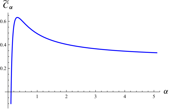
Figure 5: Plot of the constant term $\widetilde{C}_{\alpha}$ in Eq. (58).

It also follows from Eq. (62) that $\widetilde{C}_{\alpha}\to-\infty$ as $\alpha\to 0+$, and that when $\alpha\to\infty$ $\widetilde{C}_{\alpha}$ tends to a finite (nonzero) limit, given by

$$\widetilde{C}_{\infty}=\int_{0}^{\infty}\bigg{(}\frac{1}{t}\,\operatorname{csch}t-\operatorname{csch}^{2}t-\frac{\mathrm{e}^{-2t}}{6}\bigg{)}\frac{\mathrm{d}t}{t}\simeq 0.27970\,.$$

Taking the $\alpha\to 1$ limit in the previous formulas we obtain the following asymptotic expression for the von Neumann entropy $S\equiv S_{1}$:

$$S\simeq\frac{m+1}{3}\,\log L+C_{1}\,,$$ (63)

where

$$C_{1}=\frac{1}{3}\log f(p_{0},\dots,p_{m})+(m+1)\widetilde{C}_{1}$$

and the universal constant $\widetilde{C}_{1}\equiv\lim_{\alpha\to 1}\widetilde{C}_{\alpha}$ is given by

$$\widetilde{C}_{1}=\int_{0}^{\infty}\bigg{(}\frac{\cosh t}{\sinh^{3}t}-\frac{1}{t\sinh^{2}t}-\frac{\mathrm{e}^{-2t}}{3t}\bigg{)}\mathrm{d}t\simeq 0.495018\,.$$

Note, in particular, that the latter equation agrees with the formula for the analogous constant $\varUpsilon_{1}$ in Ref. Jin and Korepin (2004).

The formula (58)-(62) (or its counterpart (63) for the von Neumann entropy) provides an excellent approximation to the ground-state Rényi entanglement entropy of the supersymmetric chain (3) for even moderately large values of $L$. As an example, in Fig. 6 we have represented the relative error $r_{L}\equiv S_{\mathrm{app}}/S-1$, where $S_{\mathrm{app}}$ is the approximation (63) to the von Neumann entropy $S$, for the finite-range chain (22) in the case $J=1/2$ and $\mu=17/4$. The value of $S$ has been numerically computed diagonalizing the correlation matrix $A_{L}$ and using the exact formula (36) (with $\alpha=1$). As explained in Section III, for the value of $J$ considered the dispersion relation has exactly one maximum in the interval $(0,\pi)$, and hence is not monotonic. In particular, for $\mu\in({\mathcal{E}}(\pi),{\mathcal{E}}_{\text{max}})=(4,9/2)$ the Fermi sea consists of two disjoint intervals, as is also apparent from the inset in Fig. 6. As can be seen from the latter figure, the relative error decreases (though not monotonically) from $2.5\times 10^{-5}$ to $10^{-6}$ when $L$ ranges from $100$ to $500$.

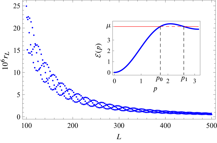
Figure 6: Relative error $r_{L}\equiv S_{\mathrm{app}}/S-1$ of the approximation $S_{\mathrm{app}}$ in the RHS of Eq. (63) to the von Neumann ground-state entanglement entropy of the chain (22) with $J=1/2$ and $\mu=17/4$ as a function of the block length $L$. Inset: dispersion relation of the chain (22) with the latter values of $J$ and $\mu$. (The interval $({\mathcal{E}}(\pi),{\mathcal{E}}_{\text{max}})$ is in this case is $(4,9/2)$, $m=1$, $p_{0}\simeq 1.71777$ and $p_{1}\simeq 2.59356$.)

VI Conclusions and outlook

In this paper we have analyzed the critical behavior of a large class of supersymmetric spin chains whose dispersion relation ${\mathcal{E}}(p)$ is not assumed to be monotonic in the interval $[0,\pi]$. We have examined the conditions under which the dispersion relation is well-defined (i.e., is a continuous function) in the thermodynamic limit, providing several simple examples of models of this type, with both short- and long-range interactions, whose dispersion relation is not monotonic.

The main conclusion of our work is that the criticality properties of the supersymmetric chains (3) are determined exclusively by the topology (the number of points) of their Fermi “surface”. More precisely, through the analysis of the free energy per spin in the critical (gapless) phase, we have shown that these models are equivalent to a system of $m+1$ free bosons with Fermi velocities $v_{i}={\mathcal{E}}^{\prime}(p_{i})$, where $p_{0},\dots,p_{m}$ are the points of the Fermi surface in the interval $[0,\pi]$. In particular, the central charge is equal to the number $m+1$ of connected components (intervals) of the Fermi sea. This result is corroborated by the asymptotic behavior of the ground-state Rényi entanglement entropy $S_{\alpha}$ as the block size $L$ tends to infinity, which has been derived applying a proved case of the Fisher–Hartwig conjecture. Indeed, we have shown that $S_{\alpha}\simeq(m+1)(1+\alpha^{-1})\log L+C_{\alpha}$, where $C_{\alpha}$ is a nonuniversal constant (independent of $L$) which we have computed in closed form in terms of the momenta $p_{0},\dots,p_{m}$. In particular, for large $L$ the entanglement entropy exhibits the logarithmic growth characteristic of $(1+1)$-dimensional conformal field theories with central charge $c=m+1$. This behavior, which is typical of critical (fermionic) one-dimensional lattice models with short-range interactions (see, e.g., Eisert et al. (2010); Ares et al. (2014a)), was recently established by the authors for supersymmetric spin chains of the type considered here under the assumption that the dispersion relation is monotonic in $[0,\pi]$.

The present work opens up several possible lines for future research. In the first place, one could consider a generalization of our results on the ground-state entanglement entropy to more general situations (for instance, considering excited states, as in Ref. Ares et al. (2014a)), in which the Fermi sea is not necessarily a finite union of disjoint intervals but exhibits a more complicated topological structure. Another interesting generalization of the present work is the analysis of the entanglement of a subset consisting of the union of two or more disjoint blocks. In fact, the entanglement entropy of this type of subsystems has already been discussed in Ref. Ares et al. (2014b), giving rise to an unproved conjecture on the asymptotic behavior of the determinant of a block Toeplitz matrix.

Appendix A Toeplitz matrices and the Fisher–Hartwig conjecture

In this appendix we shall briefly review the Fisher–Hartwig conjecture on the asymptotic behavior of the determinant of a Toeplitz matrix when its order tends to infinity. (Recall that a matrix $T$ is Toeplitz if its matrix elements $t_{ij}$ depend only on $i-j$.)

If $c(z)$ is a (complex-valued) function defined on the unit circle $S^{1}=\{z\in{\mathbb{C}}:|z|=1\}$ , we define its Fourier coefficients $c_{n}$ ($n\in{\mathbb{Z}}$) by

$$c_{n}=\frac{1}{2\pi\mathrm{i}}\int_{|z|=1}c(z)\,z^{-n-1}\,\mathrm{d}z\equiv\frac{1}{2\pi}\int_{0}^{2\pi}c\bigl{(}\mathrm{e}^{\mathrm{i}\theta}\bigr{)}\mathrm{e}^{-\mathrm{i}n\theta}\,\mathrm{d}\theta\,.$$

Note that the last integral can in fact be extended to any interval of length $2\pi$, by the $2\pi$-periodicity of the integrand. For any $L\in{\mathbb{N}}$, the function $c:S^{1}\to{\mathbb{C}}$ defines a Toeplitz matrix $T_{L}$ of order $L$ through the relation

$$(T_{L})_{ij}=c_{i-j}\,,\qquad 1\leqslant i,j\leqslant L\,.$$

We shall say that the function $c$ is the symbol of the Toeplitz matrix $T_{L}$. The Fisher–Hartwig conjecture applies to matrices $T_{L}$ whose symbol satisfies certain requirements that we shall next describe.

More precisely Ehrhardt and Silbermann (1997), $c$ should be of the form

$$c(z)=b(z)\prod_{r=1}^{R}t_{\beta_{r}}\bigl{(}\mathrm{e}^{\mathrm{i}(\theta-\theta_{r})}\bigr{)}\big{[}2-2\cos(\theta-\theta_{r})\big{]}^{\alpha_{r}}\,,$$ (64)

where $\operatorname{Re}\alpha_{r}>-1/2$, $b:S^{1}\to{\mathbb{C}}$ is a nonvanishing smooth function with zero winding number and

$$t_{\beta}(z)=\mathrm{e}^{\mathrm{i}\beta(\theta-\pi)}\,,\qquad\theta\equiv\arg_{[0,2\pi)}z\,.$$ (65)

Note that $t_{\beta}(\mathrm{e}^{\mathrm{i}(\theta-\theta_{0}})$ has in general (i.e., unless $\beta$ is an integer) a single jump discontinuity at $z=\mathrm{e}^{\mathrm{i}\theta_{0}}$. If $c$ satisfies Eq. (64), we denote by $l_{n}$ ($n\in{\mathbb{Z}}$) the $n$-th Fourier coefficient of $\log b$ (which is well defined and smooth, from the smoothness of $b$ and the assumption on its winding number), and define

$$b_{\pm}(z)=\exp\bigg{(}\sum_{n=1}^{\infty}l_{\pm n}z^{\pm n}\bigg{)}\,,\qquad z\in S_{1}\,.$$

It is immediate to show that $b_{+}$ (resp. $b_{-}$) can be analytically prolonged to the interior (resp. exterior) of the unit circle. It also follows from the definition of $b_{\pm}$ that on the unit circle we have the Wiener–Hopf decomposition

$$b(z)=\mathrm{e}^{l_{0}}b_{+}(z)b_{-}(z)\,,\qquad z\in S^{1}\,.$$

Let us further set

$$E[b]=\exp\bigg{(}\sum_{n=1}^{\infty}n\,l_{n}l_{-n}\bigg{)}$$

and

$$E =E[b]\prod_{r=1}^{R}b_{+}\bigl{(}\mathrm{e}^{\mathrm{i}\theta_{r}}\bigr{)}^{\beta_{r}-\alpha_{r}}b_{-}\bigl{(}\mathrm{e}^{\mathrm{i}\theta_{r}}\bigr{)}^{-\alpha_{r}-\beta_{r}}$$

$$\hphantom{={}}\times\prod_{1\leqslant s\neq r\leqslant R}\big{(}1-\mathrm{e}^{\mathrm{i}(\theta_{s}-\theta_{r})}\big{)}^{(\alpha_{r}+\beta_{r})(\beta_{s}-\alpha_{s})}$$

$$\hphantom{={}}\times\prod_{r=1}^{R}\frac{G(1+\alpha_{r}+\beta_{r})G(1+\alpha_{r}-\beta_{r})}{G(1+2\alpha_{r})}\,,$$

where the Barnes $G$-function is the entire function defined by

$$G(1+z)=(2\pi)^{\frac{z}{2}}\mathrm{e}^{-(z+1)\frac{z}{2}-\gamma_{E}\frac{z^{2}}{2}}\prod_{n=1}^{\infty}\bigg{[}\bigg{(}1+\frac{z}{n}\bigg{)}^{\!n}\mathrm{e}^{-z+\frac{z^{2}}{2n}}\bigg{]}$$

and $\gamma_{E}$ is the Euler–Mascheroni constant. The Fisher–Hartwig conjecture states Ehrhardt and Silbermann (1997) that if $T_{L}$ is the Toeplitz matrix with symbol (64) then when $L\to\infty$ we have

$$\det T_{L}=\mathrm{e}^{l_{0}L}L^{M}E\big{(}1+o(1)\big{)}\,,$$

with

$$M=\sum_{r=1}^{R}(\alpha_{r}^{2}-\beta_{r}^{2})\,.$$

The above conjecture was actually proved by Böttcher and Silbermann Böttcher and Silbermann (1985) in the case

$$|\operatorname{Re}\alpha_{r}|<\frac{1}{2}\,,\quad|\operatorname{Re}\beta_{r}|<\frac{1}{2}\,,\qquad r=1,\dots,R\,,$$

which, as we shall see below, is the relevant one for our purposes. In fact, as explained in Section V, we shall only need to consider the case in which $\alpha_{r}=0$ for all $r$ and $b$ is a constant (i.e., independent of $\theta$). The Fisher–Hartwig conjecture simplifies considerably in this case, since

$$l_{n}=l_{0}\,\delta_{0n}\implies b_{\pm}=E[b]=1\,,\quad\mathrm{e}^{l_{0}}=b\,,$$

and therefore

$$\det T_{L}=b^{L}L^{M}E\big{(}1+o(1)\big{)}$$ (66)

with

$$M=-\sum_{r=1}^{R}\beta_{r}^{2}$$ (67)

and

$$E=\prod_{1\leqslant s<r\leqslant R}\left(2\left|\sin\bigl{(}\tfrac{\theta_{r}-\theta_{s}}{2}\bigr{)}\right|\right)^{2\beta_{r}\beta_{s}}\\ \times\prod_{r=1}^{R}G(1+\beta_{r})G(1-\beta_{r})\,.$$ (68)

Note also that the product $G(1+z)G(1-z)$ reduces to

$$G(1+z)G(1-z)=\mathrm{e}^{-(1+\gamma_{E})z^{2}}\prod_{n=1}^{\infty}\bigg{[}\bigg{(}1-\frac{z^{2}}{n^{2}}\bigg{)}^{n}\mathrm{e}^{\frac{z^{2}}{n}}\bigg{]}\,.$$ (69)

We shall be mainly interested in the case in which $T_{L}=\lambda-(2A_{L}-\openone)$, where $\lambda$ is a spectral parameter and $A_{L}$ is the correlation matrix of a block of $L$ spins of the $\mathrm{su}(1|1)$ supersymmetric spin chain. As a first example, let us express in the form (64)-(65) the symbol of the matrix $T_{L}$ when the chain’s dispersion relation is monotonic in the interval $[0,\pi]$. To begin with, in this case we have

$$(A_{L})_{jk}=\frac{\sin(p_{0}(j-k))}{\pi(j-k)}=\frac{1}{2\pi}\int_{-p_{0}}^{p_{0}}\mathrm{e}^{-\mathrm{i}(j-k)\theta}\,\mathrm{d}\theta,$$

where $p_{0}\in[0,\pi]$ is the Fermi momentum Carrasco et al. (2016b). Thus the symbol of the Toeplitz matrix $A_{L}$ is

$$f\bigl{(}\mathrm{e}^{\mathrm{i}\theta}\bigr{)}=\begin{cases}1\,,\quad&-p_{0}<\theta<p_{0}\,,\\ 0\,,&p_{0}<\theta<2\pi-p_{0}\,,\end{cases}$$

and that of $T_{L}$ is therefore given by

$$c\bigl{(}\mathrm{e}^{\mathrm{i}\theta}\bigr{)}=\begin{cases}\lambda-1\,,\quad&-p_{0}<\theta<p_{0}\,,\\ \lambda+1\,,&p_{0}<\theta<2\pi-p_{0}\,.\end{cases}$$

Note that $c$ has two jump discontinuities on the unit circle at the points $\mathrm{e}^{\pm\mathrm{i}p_{0}}$. We shall next show that

$$c\bigl{(}\mathrm{e}^{\mathrm{i}\theta}\bigr{)}=b\bigl{(}\mathrm{e}^{\mathrm{i}\theta}\bigr{)}t_{\beta}\bigl{(}\mathrm{e}^{\mathrm{i}(\theta+p_{0})}\bigr{)}t_{-\beta}\bigl{(}\mathrm{e}^{\mathrm{i}(\theta-p_{0})}\bigr{)}$$ (70)

for suitable $\beta$ and $b(z)$. Indeed, first of all we have

$$-p_{0}<\theta<2\pi-p_{0} \implies 0<\theta+p_{0}<2\pi$$

$$\implies t_{\beta}\bigl{(}\mathrm{e}^{\mathrm{i}(\theta+p_{0})}\bigr{)}=\mathrm{e}^{\mathrm{i}\beta(\theta+p_{0}-\pi)}\,.$$

On the other hand, if $-p_{0}<\theta<p_{0}$ then

$$0\leqslant 2(\pi-p_{0})<\theta-p_{0}+2\pi<2\pi\\ \implies t_{-\beta}\bigl{(}\mathrm{e}^{\mathrm{i}(\theta-p_{0})}\bigr{)}=\mathrm{e}^{-\mathrm{i}\beta(\theta-p_{0}+\pi)}\,,$$

while for $p_{0}<\theta<2\pi-p_{0}$ we have

$$0<\theta-p_{0}<2(\pi-p_{0})\leqslant 2\pi\\ \implies t_{-\beta}\bigl{(}\mathrm{e}^{\mathrm{i}(\theta-p_{0})}\bigr{)}=\mathrm{e}^{-\mathrm{i}\beta(\theta-p_{0}-\pi)}\,.$$

Hence

$$t_{\beta}\bigl{(}\mathrm{e}^{\mathrm{i}(\theta+p_{0})}\bigr{)} t_{-\beta}\bigl{(}\mathrm{e}^{\mathrm{i}(\theta-p_{0})}\bigr{)}$$ (71)

$$=\begin{cases}\mathrm{e}^{2\mathrm{i}\beta(p_{0}-\pi)}\,,&-p_{0}<\theta<p_{0}\,,\\ \mathrm{e}^{2\mathrm{i}\beta p_{0}}\,,&p_{0}<\theta<2\pi-p_{0}\,.\end{cases}$$

In order for Eq. (70) to hold we must therefore have

$$b\,\mathrm{e}^{2\mathrm{i}\beta(p_{0}-\pi)}=\lambda-1\,,\qquad b\,\mathrm{e}^{2\mathrm{i}\beta p_{0}}=\lambda+1\,,$$

from which we easily get

$$\mathrm{e}^{2\mathrm{i}\beta\pi}=\frac{\lambda+1}{\lambda-1}\,,\qquad b=(\lambda+1)\mathrm{e}^{-2\mathrm{i}\beta p_{0}}\,.$$

Although these equations admit an infinite number of solutions $(\beta,b)$ provided that $\lambda\neq\pm 1$, it will prove convenient for our purposes to take

$$\beta=\frac{1}{2\pi\mathrm{i}}\,\log\bigg{(}\frac{\lambda+1}{\lambda-1}\bigg{)}\,,\quad b=(\lambda+1)\bigg{(}\frac{\lambda+1}{\lambda-1}\bigg{)}^{-p_{0}/\pi}\,,$$ (72)

where $\log z\equiv\log|z|+\mathrm{i}\arg_{(-\pi,\pi]}z$ and $z^{a}\equiv\mathrm{e}^{a\log z}$. Note, in particular, that $b$ is a nonvanishing constant. It is also important to observe that

$$\lambda\notin[-1,1]\implies|\operatorname{Re}\beta|=\frac{1}{2\pi}\arg_{(-\pi,\pi]}\bigg{(}\frac{\lambda+1}{\lambda-1}\bigg{)}<\frac{1}{2}\,,$$

since by definition $-\pi<\arg_{(-\pi,\pi]}z\leqslant\pi$ and

$$\arg_{(-\pi,\pi]}\bigg{(}\frac{\lambda+1}{\lambda-1}\bigg{)}=\pi \iff\frac{\lambda+1}{\lambda-1}\in(-\infty,0)$$

$$\iff\lambda\in(-1,1)\,.$$

Thus the Fisher–Hartwig conjecture can be applied provided that $\lambda$ lies outside the closed interval $[-1,1]$, with $R=1$, $\alpha_{1}=0$ and

$$M=-2\beta^{2}\,,\qquad E=\big{(}2\sin p_{0}\big{)}^{-2\beta^{2}}G(1+\beta)^{2}G(1-\beta)^{2}\,.$$

By Eqs. (66) and (72), when $L\to\infty$ the characteristic polynomial $D_{L}(\lambda)\equiv\det(\lambda+1-2A_{L})$ is given by

$$D_{L}(\lambda)=\big{(}2L\sin p_{0}\big{)}^{-2\beta^{2}}(\lambda+1)^{L}\bigg{(}\frac{\lambda+1}{\lambda-1}\bigg{)}^{-Lp_{0}/\pi}\\ \times G(1+\beta)^{2}G(1-\beta)^{2}\big{(}1+o(1)\big{)}\,,$$ (73)

with $\beta$ defined by Eq. (72). This is precisely the formula used by Jin and Korepin Jin and Korepin (2004) for the determination of the asymptotic behavior of the ground state entanglement entropy of the $X\!X$ model.

As a second example, we shall consider a simple case in which the dispersion relation ${\mathcal{E}}$ is not monotonic in $[0,\pi]$. More precisely, suppose that ${\mathcal{E}}$ is nonnegative and has a single maximum in the open interval $(0,\pi)$ (cf. Fig. 7).

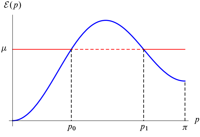
Figure 7: Dispersion relation ${\mathcal{E}}(p)$ with a single maximum in $(0,\pi)$.

For $\mu\in(0,{\mathcal{E}}(\pi))$, the equation ${\mathcal{E}}(p)=\mu$ has one root $p_{0}$ in the interval $(0,\pi)$, and the determinant $D_{L}(\lambda)$ is approximately given by Eq. (73). We shall next determine the asymptotic behavior of $D_{L}(\lambda)$ when $\mu\in({\mathcal{E}}(\pi),{\mathcal{E}}_{\mathrm{max}})$, where ${\mathcal{E}}_{\text{max}}$ is the maximum value of ${\mathcal{E}}(p)$, and thus the equation ${\mathcal{E}}(p)=\mu$ has two roots $p_{0}<p_{1}$ in the interval $(0,\pi)$. To begin with, from Eq. (40) it follows that in this case

$$(A_{L})_{jk}=\frac{1}{2\pi}\left(\int_{-p_{0}}^{p_{0}}+\int_{p_{1}}^{2\pi-p_{1}}\right)\mathrm{e}^{-\mathrm{i}(j-k)p}\mathrm{d}p\,.$$

Thus the symbol of $T_{L}=\lambda+1-2A_{L}$ is given by

$$c\bigl{(}\mathrm{e}^{\mathrm{i}\theta}\bigr{)}=\begin{cases}\lambda-1\,,\quad&\theta\in(-p_{0},p_{0})\cup(p_{1},2\pi-p_{1})\\ \lambda+1\,,&\theta\in(p_{0},p_{1})\cup(2\pi-p_{1},2\pi-p_{0})\,.\end{cases}$$ (74)

In other words, $c\bigl{(}\mathrm{e}^{\mathrm{i}\theta}\bigr{)}$ alternatively takes on the two values $\lambda-1$ and $\lambda+1$ on each of the four intervals $(-p_{0},p_{0}),\dots,(2\pi-p_{1},2\pi-p_{0})$ on which ${\mathcal{E}}(p)-\mu$ has constant sign, starting with $\lambda-1$. Since the symbol (74) has four discontinuities at the points $\mathrm{e}^{\pm\mathrm{i}p_{0}}$ and $\mathrm{e}^{\pm\mathrm{i}p_{1}}$ , we shall try to express it as

$$c\bigl{(}\mathrm{e}^{\mathrm{i}\theta}\bigr{)}=b\bigl{(}\mathrm{e}^{\mathrm{i}\theta}\bigr{)}t_{\beta_{0}}\bigl{(}\mathrm{e}^{\mathrm{i}(\theta+p_{0})}\bigr{)}t_{-\beta_{0}}\bigl{(}\mathrm{e}^{\mathrm{i}(\theta-p_{0})}\bigr{)}\\ \times t_{\beta_{1}}\bigl{(}\mathrm{e}^{\mathrm{i}(\theta+p_{1})}\bigr{)}t_{-\beta_{1}}\bigl{(}\mathrm{e}^{\mathrm{i}(\theta-p_{1})}\bigr{)}$$ (75)

for suitably chosen $b$, $\beta_{i}$. In fact, we only need compute $t_{\pm\beta_{1}}\bigl{(}\mathrm{e}^{\mathrm{i}(\theta\pm p_{1})}\bigr{)}$, which is straightforward:

$$t_{\beta_{1}}\bigl{(}\mathrm{e}^{\mathrm{i}(\theta+p_{1})}\bigr{)} =\begin{cases}\mathrm{e}^{\mathrm{i}\beta_{1}(\theta+p_{1}-\pi)}\,,\enspace&-p_{0}<\theta<2\pi-p_{1}\\ \mathrm{e}^{\mathrm{i}\beta_{1}(\theta+p_{1}-3\pi)}\,,&2\pi-p_{1}<\theta<2\pi-p_{0}\end{cases}$$

$$t_{-\beta_{1}}\bigl{(}\mathrm{e}^{\mathrm{i}(\theta-p_{1})}\bigr{)} =\begin{cases}\mathrm{e}^{-\mathrm{i}\beta_{1}(\theta-p_{1}+\pi)}\,,\enspace&-p_{0}<\theta<p_{1}\\ \mathrm{e}^{-\mathrm{i}\beta_{1}(\theta-p_{1}-\pi)}\,,&p_{1}<\theta<2\pi-p_{0}\,.\end{cases}$$

Combining the previous equations with Eq. (71) and comparing with Eq. (74) we immediately arrive at the system

$$b\,\mathrm{e}^{2\mathrm{i}(\beta_{0}p_{0}+\beta_{1}p_{1})}\mathrm{e}^{-2\pi\mathrm{i}(\beta_{0}+\beta_{1})}=b\,\mathrm{e}^{2\mathrm{i}(\beta_{0}p_{0}+\beta_{1}p_{1})}=\lambda-1$$

$$b\,\mathrm{e}^{2\mathrm{i}(\beta_{0}p_{0}+\beta_{1}p_{1})}\mathrm{e}^{-2\pi\mathrm{i}\beta_{1}}=\lambda+1\,.$$

From the first equation it follows that $\beta_{0}+\beta_{1}$ must be an integer. Choosing the simplest solution $\beta_{0}=-\beta_{1}\equiv\beta$ and dividing the last equation by the first one we again obtain Eq. (72) for $\beta$. Finally, from the last equation it follows that

$$b=(\lambda+1)\mathrm{e}^{2\mathrm{i}\beta(p_{1}-p_{0}-\pi)}=(\lambda+1)\bigg{(}\frac{\lambda+1}{\lambda-1}\bigg{)}^{(p_{1}-p_{0}-\pi)/\pi}\,.$$ (76)

Note that $\beta$ is still given by Eq. (72), so the condition $|\operatorname{Re}\beta|<1/2$, necessary for the validity of the Fisher–Hartwig conjecture, also applies in this case if $\lambda\notin[-1,1]$. Since now $M=-4\beta^{2}$,

$$\prod_{r=1}^{4}G(1+\beta_{r})G(1-\beta_{r})=G(1+\beta)^{4}G(1-\beta)^{4}$$

and

$$\prod_{1\leqslant s<r\leqslant 4}\big{(}2|\sin\bigl{(}\tfrac{\theta_{r}-\theta_{s}}{2}\bigr{)}|\big{)}^{2\beta_{r}\beta_{s}}\\ =\big{(}2\sin\bigl{(}\tfrac{p_{1}-p_{0}}{2}\bigr{)}\big{)}^{-4\beta^{2}}\big{(}2\sin\bigl{(}\tfrac{p_{1}+p_{0}}{2}\bigr{)}\big{)}^{4\beta^{2}}\\ \times(4\sin p_{0}\sin p_{1})^{-2\beta^{2}}\,.$$

By the Fisher–Hartwig conjecture, the determinant $D_{L}(\lambda)$ is given in this case by

$$D_{L}(\lambda) =\bigg{[}\frac{4L^{2}\sin p_{0}\sin p_{1}\sin^{2}\bigl{(}\tfrac{p_{1}-p_{0}}{2}\bigr{)}}{\sin^{2}\bigl{(}\tfrac{p_{1}+p_{0}}{2}\bigr{)}}\bigg{]}^{\!\!-2\beta^{2}}$$

$$\hphantom{={}\bigg{(}}\times(\lambda+1)^{L}\bigg{(}\frac{\lambda+1}{\lambda-1}\bigg{)}^{\frac{L}{\pi}(p_{1}-p_{0}-\pi)}$$

$$\hphantom{={}\bigg{(}}\times G(1+\beta)^{4}G(1-\beta)^{4}\big{(}1+o(1)\big{)}\,.$$ (77)

Appendix B Computation of the integral $I_{1}(\alpha)$

In this appendix we shall provide an elementary derivation of the integral $I_{1}(\alpha)$ in Eq. (55), which appears in the asymptotic expression of the Rényi entanglement entropy of the model (3). To begin with, we have

$$I_{1}(\alpha)=\frac{2}{\pi^{2}}(1-\alpha)^{-1}\hat{I}_{1}(\alpha)\,,$$

with

$$\hat{I}_{1}(\alpha)=\int_{-1}^{1}\log\biggl{[}\bigg{(}\frac{1+x}{2}\bigg{)}^{\alpha}+\bigg{(}\frac{1-x}{2}\bigg{)}^{\alpha}\biggr{]}\,\frac{\mathrm{d}x}{1-x^{2}}\,,$$

or equivalently (performing the change of variables $t=(x+1)/2$)

$$\hat{I}_{1}(\alpha)=\int_{0}^{1}\log\bigl{[}t^{\alpha}+(1-t)^{\alpha}\bigr{]}\frac{\mathrm{d}t}{t}\,.$$ (78)

Integrating by parts we obtain the equivalent expression

$$\hat{I}_{1}(\alpha)=-\alpha\int_{0}^{1}\frac{t^{\alpha-1}-(1-t)^{\alpha-1}}{t^{\alpha}+(1-t)^{\alpha}}\,\log t\,\mathrm{d}t\,.$$ (79)

On the other hand, differentiating Eq. (78) with respect to $\alpha$ we easily get

$$\hat{I}_{1}^{\prime}(\alpha)=\int_{0}^{1}\frac{t^{\alpha-1}}{t^{\alpha}+(1-t)^{\alpha}}\,\frac{\log t}{1-t}\,\mathrm{d}t\,,$$

and hence Olver et al. (2010)

$$\hat{I}_{1}^{\prime}(\alpha)+\frac{\hat{I}_{1}(\alpha)}{\alpha}=\int_{0}^{1}\frac{\log t}{1-t}\,\mathrm{d}t=-\frac{\pi^{2}}{6}\,.$$

Solving this linear differential equation with the initial condition $\hat{I}_{1}(1)=0$ we finally obtain

$$\hat{I}_{1}(\alpha)=\frac{\pi^{2}}{12\alpha}\,(1-\alpha^{2})\,,$$ (80)

which immediately yields Eq. (57).

Appendix C Simplification of the constant $\widetilde{C}_{\alpha}$

In this appendix we derive Eq. (61) for the constant $\widetilde{C}_{\alpha}$ in Eq. (58), and show that it can be more simply expressed by means of the integral (62). To this end, we use the elementary identity

$$\psi(z)=-\gamma_{E}+\sum_{n=1}^{\infty}\bigg{(}\frac{1}{n}-\frac{1}{n+z-1}\bigg{)}\,,$$

which can be immediately derived from the well-known infinite product for the Gamma function. Our starting point is the definition (56) of $I_{2}(\alpha)$, which can be written as

$$I_{2}(\alpha)=\frac{2}{\pi^{2}}\int_{-1}^{1}\frac{s_{\alpha}(x)}{1-x^{2}}\big{[}f\bigl{(}Z(x)\bigr{)}+f\bigl{(}1-Z(x)\bigr{)}\big{]}\mathrm{d}x\,,$$ (81)

with $Z(x)=1/2+\mathrm{i}B(x)$ and

$$f(z)=\sum_{n=1}^{\infty}\frac{z^{3}}{n(n^{2}-z^{2})}\,.$$

From the relation

$$\frac{z^{2}}{n(z^{2}-n^{2})}=\frac{1}{2}\bigg{(}\frac{1}{n+z}-\frac{1}{n}\bigg{)}+\frac{1}{2}\bigg{(}\frac{1}{n-z}-\frac{1}{n}\bigg{)}$$

and the functional identity $\psi(z+1)=\psi(z)+1/z$ satisfied by the digamma function it immediately follows that

$$f(z)=-\frac{z}{2}\,\big{[}\psi(z)+\psi(1-z)\big{]}-z\gamma_{E}-\frac{1}{2}\,,$$

and therefore

$$f(z)+f(1-z)=-1-\gamma_{E}-\frac{1}{2}\,\big{[}\psi(z)+\psi(1-z)\big{]}\,.$$

Substituting into Eq. (81) and using Eqs. (57) and (59) we easily obtain Eq. (61).

In order to prove Eq. (62), we first make the change of variable $w=B(x)$ in Eq. (61), which yields

$$(1-\alpha)\widetilde{C}_{\alpha}=-\frac{2}{\pi}\int_{0}^{\infty}\log\biggl{[}\frac{2\cosh(\pi\alpha w)}{\big{(}2\cosh(\pi w)\big{)}^{\alpha}}\biggr{]}$$

$$\kern 90.00014pt\times\big{[}\psi\bigl{(}\tfrac{1}{2}+\mathrm{i}\,w\bigr{)}+\psi\bigl{(}\tfrac{1}{2}-\mathrm{i}\,w\bigr{)}\big{]}\,\mathrm{d}w$$

$$=\frac{2}{\mathrm{i}\pi}\int_{0}^{\infty}\log\biggl{[}\frac{2\cosh(\pi\alpha w)}{\big{(}2\cosh(\pi w)\big{)}^{\alpha}}\biggr{]}\frac{\mathrm{d}}{\mathrm{d}w}\log\bigg{[}\frac{\Gamma\bigl{(}\tfrac{1}{2}-\mathrm{i}\,w\bigr{)}}{\Gamma\bigl{(}\tfrac{1}{2}+\mathrm{i}\,w\bigr{)}}\bigg{]}\,\mathrm{d}w\,.$$

We next integrate by parts, taking into account that by Stirling’s formula we have

$$\log\bigg{[}\frac{\Gamma\bigl{(}\tfrac{1}{2}-\mathrm{i}\,w\bigr{)}}{\Gamma\bigl{(}\tfrac{1}{2}+\mathrm{i}\,w\bigr{)}}\bigg{]}=O(w\log w)$$

while

$$\log\biggl{[}\frac{2\cosh(\pi\alpha w)}{\big{(}2\cosh(\pi w)\big{)}^{\alpha}}\biggr{]}=O\bigl{(}\mathrm{e}^{-2\pi\min(1,\alpha)w}\bigr{)}\,,$$

so that the boundary term vanishes. We thus obtain

$$(1-\alpha)\widetilde{C}_{\alpha}\\ =2\mathrm{i}\alpha\int_{0}^{\infty}\!\big{[}\tanh(\pi\alpha w)-\tanh(\pi w)\big{]}\log\bigg{[}\frac{\Gamma\bigl{(}\tfrac{1}{2}-\mathrm{i}\,w\bigr{)}}{\Gamma\bigl{(}\tfrac{1}{2}+\mathrm{i}\,w\bigr{)}}\bigg{]}\mathrm{d}w\,.$$

On the other hand, from Gauss’s integral representation of the digamma function Whittaker and Watson (1927)

$$\psi(z)=\int_{0}^{\infty}\bigg{(}\frac{\mathrm{e}^{-t}}{t}-\frac{\mathrm{e}^{-zt}}{1-\mathrm{e}^{-t}}\bigg{)}\,\mathrm{d}t$$

it easily follows that

$$\log\Gamma(z)=\int_{0}^{\infty}\bigg{[}z-1-\frac{1-\mathrm{e}^{-(z-1)t}}{1-\mathrm{e}^{-t}}\bigg{]}\frac{\mathrm{e}^{-t}}{t}\,\mathrm{d}t$$

and hence

$$\log\bigg{[}\frac{\Gamma\bigl{(}\tfrac{1}{2}-\mathrm{i}\,w\bigr{)}}{\Gamma\bigl{(}\tfrac{1}{2}+\mathrm{i}\,w\bigr{)}}\bigg{]}=\mathrm{i}\int_{0}^{\infty}\bigg{[}\operatorname{csch}(t/2)\sin(wt)-2w\mathrm{e}^{-t}\bigg{]}\frac{\mathrm{d}t}{t}\,.$$

Substituting into the last formula for $\widetilde{C}_{\alpha}$ and using the elementary identity

$$\tanh(\pi\alpha w)-\tanh(\pi w)=\frac{2\mathrm{e}^{-2\pi w}}{1+\mathrm{e}^{-2\pi w}}-\frac{2\mathrm{e}^{-2\pi\alpha w}}{1+\mathrm{e}^{-2\pi\alpha w}}$$

we obtain

$$(1-\alpha)\widetilde{C}_{\alpha}=4\alpha\int_{0}^{\infty}\frac{g_{1}(t)-g_{\alpha}(t)}{t}\,\mathrm{d}t\,,$$

with

$$g_{\alpha}(t)=\int_{0}^{\infty}\frac{\mathrm{e}^{-2\pi\alpha w}}{1+\mathrm{e}^{-2\pi\alpha w}}\big{[}2w\mathrm{e}^{-t}-\operatorname{csch}(t/2)\sin(wt)\big{]}\mathrm{d}w.$$

The latter integral can be evaluated in closed form by elementary means. Indeed,

$$\int_{0}^{\infty}\frac{w\,\mathrm{e}^{-2\pi\alpha w}}{1+\mathrm{e}^{-2\pi\alpha w}}\mathrm{d}w=\sum_{n=1}^{\infty}(-1)^{n+1}\int_{0}^{\infty}w\,\mathrm{e}^{-2n\pi\alpha w}\mathrm{d}w$$

$$=\frac{1}{4\pi^{2}\alpha^{2}}\sum_{n=1}^{\infty}\frac{(-1)^{n+1}}{n^{2}}=\frac{\zeta(2)}{8\pi^{2}\alpha^{2}}=\frac{1}{48\alpha^{2}}\,,$$

while

$$\int_{0}^{\infty}\frac{\mathrm{e}^{\mathrm{i}wt}\,\mathrm{e}^{-2\pi\alpha w}}{1+\mathrm{e}^{-2\pi\alpha w}}\mathrm{d}w=\sum_{n=1}^{\infty}(-1)^{n+1}\int_{0}^{\infty}\mathrm{e}^{(\mathrm{i}t-2n\pi\alpha)w}\mathrm{d}w$$

$$=\sum_{n=1}^{\infty}\frac{(-1)^{n}}{\mathrm{i}\,t-2n\pi\alpha}\,,$$

and therefore

$$\int_{0}^{\infty}\frac{\mathrm{e}^{-2\pi\alpha w}\sin(wt)}{1+\mathrm{e}^{-2\pi\alpha w}}\mathrm{d}w=\operatorname{Im}\sum_{n=1}^{\infty}\frac{(-1)^{n}}{\mathrm{i}\,t-2n\pi\alpha}$$

$$=t\sum_{n=1}^{\infty}\frac{(-1)^{n+1}}{t^{2}+4\alpha^{2}\pi^{2}n^{2}}=\frac{1}{4\alpha}\bigg{(}\frac{2\alpha}{t}-\operatorname{csch}\bigl{(}t/(2\alpha)\bigr{)}\bigg{)}.$$

We thus obtain

$$g_{\alpha}(t)=\frac{\mathrm{e}^{-t}}{24\alpha^{2}}+\operatorname{csch}(t/2)\bigg{(}\frac{\operatorname{csch}\bigl{(}t/(2\alpha)\bigr{)}}{4\alpha}-\frac{1}{2t}\bigg{)}\,,$$

from which Eq. (62) easily follows.